Hyperbolic-like elastic scattering of spinning particles by a Schwarzschild black hole

Abstract

The scattering of spinning test particles by a Schwarzschild black hole is studied. The motion is described according to the Mathisson-Papapetrou-Dixon model for extended bodies in a given gravitational background field. The equatorial plane is taken as the orbital plane, the spin vector being orthogonal to it with constant magnitude. The equations of motion are solved analytically in closed form to first-order in spin and the solution is used to compute corrections to the standard geodesic scattering angle as well as capture cross section by the black hole.

1 Introduction

After the discovery of the gravitational waves in 2015 Abbott:2016blz a new window in gravitational physics was opened, looking for any suitable astrophysical situation which could lead to the detection of new events. Binary systems in this sense play a central role. Indeed, the first detection has concerned a binary black hole system, whose evolution has been followed along all inspiral-coalescing-merging-plunging phases. Another promising situation is that of hyperbolic encounters or scattering by two black holes. This problem is, in principle, as interesting as the previous one, but its description is more complicated. For example, an almost circularized binary system emits gravitational waves at the frequency of its orbital motion and hence has its spectrum very compact around that value. The spectrum associated with a hyperbolic scattering of two black holes, instead, covers a large range of frequencies, and the theoretical predictions in terms of observed flux have not been developed much beyond the pioneering works of the 70’s rr-wheeler ; Rees:1974iy , so that most of the existing analysis belongs to lowest-order Post-Newtonian approximation Blanchet:1989cu and numerical relativity Pretorius:2007jn ; Shibata:2008rq ; Sperhake:2008ga ; Sperhake:2009jz ; Sperhake:2012me . Semi-analytical methods, like the Effective-One-Body formalism, are trying to fill the gap, but no results beyond the 3PN approximation level have been shown in the literature up to now Majar:2010em ; Bini:2012ji ; Damour:2014afa ; DeVittori:2014psa .

We study here the problem of scattering of a spinning test particle by a Schwarzschild black hole according to the Mathisson-Papapetrou-Dixon (MPD) model Mathisson:1937zz ; Papapetrou:1951pa ; Dixon:1970zza , in comparison with the well known case of spinless particles moving along hyperbolic-like geodesic orbits. The equatorial plane is chosen as the orbital plane, implying that the spin vector is orthogonal to it with constant magnitude, as a consequence of the MPD equations. Taking advantage of the condition of “small spin” implicit in the MPD model to avoid backreaction effects on the background metric as well as of the existence of conserved quantities related to Killing symmetries, we are able to analytically solve the equations of motion in terms of Elliptic integrals. We compute the corrections to first-order in spin to the scattering angle, i.e., the most natural gauge-invariant and physical observable associated with the scattering process. Using a conical-like parametrization for the radial motion we express the scattering angle in terms of eccentricity and (inverse) semi-latus rectum, the latter parameters being in a $1$-$1$ correspondence with the two other natural variables: energy and angular momentum (which are also gauge invariant variables). We also determine the modification due to spin to the capture cross section by the black hole. Finally, we compare the nongeodesic motion of a spinning particle discussed here with the companion situation of geodesic motion of a spinless particle orbiting a slowly rotating Kerr black hole in the weak field limit and discuss some reciprocity relations.

We will use geometrical units and conventionally assume that Greek indices run from $0$ to $3$, whereas Latin indices run from $1$ to $3$.

2 Equatorial plane motion in a Schwarzschild spacetime

The motion of a spinning test particle in a given gravitational background is described by the MPD equations Mathisson:1937zz ; Papapetrou:1951pa ; Dixon:1970zza

$$\frac{DP^{\mu}}{d\tau} = -\frac{1}{2}\,R^{\mu}{}_{\nu\alpha\beta}\,U^{\nu}\,S^{\alpha\beta}\equiv F^{\mu}_{\rm(spin)}\,,$$ (1)

$$\frac{DS^{\mu\nu}}{d\tau} = 2\,P^{[\mu}U^{\nu]}\,,$$ (2)

where $P^{\mu}\equiv mu^{\mu}$ (with $u\cdot u\equiv u^{\mu}u_{\mu}=-1$) is the total 4-momentum of the body with mass $m$ and unit direction $u^{\mu}$, $S^{\mu\nu}$ is the (antisymmetric) spin tensor, and $U^{\mu}=dx^{\mu}/d\tau$ is the timelike unit 4-velocity vector tangent to the body “center-of-mass line,” parametrized by the proper time $\tau$ (with parametric equations $x^{\mu}=x^{\mu}(\tau)$), used to make the multipole reduction.

In order to ensure that the model is mathematically self-consistent, the reference world line in the object should be specified by imposing some additional conditions. Here we shall use the Tulczyjew-Dixon conditions Dixon:1970zza ; tulc59 , which read

$$S^{\mu\nu}u{}_{\nu}=0\,.$$ (3)

With this choice, the spin tensor can be fully represented by a spatial vector (with respect to $u$),

$$S(u)^{\alpha}=\frac{1}{2}\eta(u)^{\alpha}{}_{\beta\gamma}S^{\beta\gamma}\,,$$ (4)

where $\eta(u)_{\alpha\beta\gamma}=\eta_{\mu\alpha\beta\gamma}u^{\mu}$ is the spatial unit volume 3-form (with respect to $u$) built from the unit volume 4-form $\eta_{\alpha\beta\gamma\delta}=\sqrt{-g}\,\epsilon_{\alpha\beta\gamma\delta}$, with $\epsilon_{\alpha\beta\gamma\delta}$ ($\epsilon_{0123}=1$) being the Levi-Civita alternating symbol and $g$ the determinant of the metric.

It is also useful to introduce the signed magnitude $s$ of the spin vector

$$s^{2}=S(u)^{\beta}S(u)_{\beta}=\frac{1}{2}S_{\mu\nu}S^{\mu\nu}\,,$$ (5)

which is a constant of motion. Implicit in the MPD model is the condition that the length scale $|s|/m$ naturally associated with the spin should be very small compared to the one associated with the background curvature (say $M$), in order to neglect back reaction effects, namely $|\hat{s}|\equiv{|s|}/{mM}\ll 1$. Introducing this smallness condition from the very beginning leads to a simplified set of linearized differential equations around the geodesic motion. In fact, the total 4-momentum $P$ of the particle is aligned with $U$ in this limit, i.e., $P^{\mu}=mU^{\mu}+O(2)$, the mass $m$ of the particle remaining constant along the path. Furthermore, Eq. (2) becomes ${DS^{\mu\nu}}/{d\tau}=O(2)$, implying that the spin vector is parallely transported along $U$.

Let us consider a spinning test particle moving in a Schwarzschild spacetime, whose metric written in standard spherical-like coordinates $(t,r,\theta,\phi)$ is

$$ds^{2}=-N^{2}dt^{2}+N^{-2}dr^{2}+r^{2}(\sin^{2}\theta d\theta^{2}+d\phi^{2})\,,$$ (6)

where $N=(1-2M/r)^{1/2}$ denotes the “lapse” function. We introduce a family of fiducial observers, the static observers with 4-velocity

$$n=N^{-1}\partial_{t}\,,$$ (7)

equipped with an adapted triad

$$e_{\hat{r}}=N\partial_{r}\,,\quad e_{\hat{\theta}}=\frac{1}{r}\partial_{\theta}\,,\quad e_{\hat{\phi}}=\frac{1}{r\sin\theta}\partial_{\phi}\,.$$ (8)

We will limit our analysis to the case of equatorial motion, i.e., $\theta=\pi/2$ is the orbital plane and hence $U^{\theta}=0$. As a convention, the physical (orthonormal) component along $-\partial_{\theta}$ which is perpendicular to the equatorial plane will be referred to as “along the positive $z$-axis” and will be indicated by the index $\hat{z}$, when convenient: $e_{\hat{z}}=-e_{\hat{\theta}}$. From the evolution equations for the spin tensor it follows that the spin vector has a single nonvanishing and constant component along $\theta$ (or $z$), namely

$$S(U)=S^{\hat{\theta}}e_{\hat{\theta}}=s\,e_{\hat{z}}\,,\qquad S^{\hat{\theta}}=-s\,.$$ (9)

Let us decompose the 4-velocity $U$ of the spinning particle with respect to the static observers

$$U=\gamma(U,n)[n+\nu(U,n)]\,,\quad\nu(U,n)\equiv\nu(U,n)^{\hat{r}}e_{\hat{r}}+\nu(U,n)^{\hat{\phi}}e_{\hat{\phi}}\,,$$ (10)

where $\gamma(U,n)=1/\sqrt{1-||\nu(U,n)||^{2}}$ is the associated Lorentz factor. Hereafter we will use the abbreviated notation $\gamma(U,n)\equiv\gamma$ and $\nu(U,n)^{\hat{a}}\equiv\nu^{\hat{a}}$. The relation with the coordinate components of $U$ is

$$U^{t}\equiv\frac{dt}{d\tau}=\frac{\gamma}{N}\,,\qquad U^{r}\equiv\frac{dr}{d\tau}=\gamma N\nu^{\hat{r}}\,,\qquad U^{\phi}\equiv\frac{d\phi}{d\tau}=\frac{\gamma\nu^{\hat{\phi}}}{r}\,.$$ (11)

The spin force turns out to be

$$F_{\rm(spin)}=\frac{3mM^{2}}{r^{3}}{\hat{s}}\gamma^{2}\nu^{\hat{\phi}}[\nu^{\hat{r}}n+e_{\hat{r}}]\,.$$ (12)

The equations of motion (1) then imply

$$\frac{d\nu^{\hat{r}}}{d\tau} = \frac{N^{2}-1}{2r\gamma N}+\gamma(\nu^{\hat{\phi}})^{2}\frac{3N^{2}-1}{2rN}-\frac{3}{2}M{\hat{s}}\frac{N^{2}-1}{\gamma r^{2}}\nu^{\hat{\phi}}[1+\gamma^{2}(\nu^{\hat{\phi}})^{2}]\,,$$

$$\frac{d\nu^{\hat{\phi}}}{d\tau} = -\frac{1}{2r^{2}N}\gamma\nu^{\hat{r}}\nu^{\hat{\phi}}\left[r(3N^{2}-1)-3M{\hat{s}}N(N^{2}-1)\nu^{\hat{\phi}}\right]\,.$$ (13)

In order to solve these equations we take advantage of the existence of conserved quantities along the motion in stationary and axisymmetric spacetimes endowed with Killing symmetries, i.e., the energy $E$ and the total angular momentum $J$ associated with the timelike Killing vector $\xi=\partial_{t}$ and the azimuthal Killing vector $\eta=\partial_{\phi}$, respectively. They are given by

$$E = -\xi_{\alpha}P^{\alpha}+\frac{1}{2}S^{\alpha\beta}\nabla_{\beta}\xi_{\alpha}\,,$$

$$J = \eta_{\alpha}P^{\alpha}-\frac{1}{2}S^{\alpha\beta}\nabla_{\beta}\eta_{\alpha}\,,$$ (14)

where $\nabla_{\beta}\xi_{\alpha}=g_{t[\alpha,\beta]}$ and $\nabla_{\beta}\eta_{\alpha}=g_{\phi[\alpha,\beta]}$. We then find

$$\hat{E}=N\gamma\left[1+\hat{s}\frac{M^{2}}{r^{2}N}\nu^{\hat{\phi}}\right]\,,\qquad\hat{J}=\frac{r}{M}\gamma\left[\nu^{\hat{\phi}}+\hat{s}N\frac{M}{r}\right]\,,$$ (15)

where $\hat{E}\equiv E/m$ and $\hat{J}\equiv J/mM$ are dimensionless. Eq. (15) thus provide two algebraic relations for the frame components $\nu^{\hat{r}}$ and $\nu^{\hat{\phi}}$ of the linear velocity, which once inserted in Eq. (11) finally yield

$$\frac{dt}{d\tau} = \frac{\hat{E}}{N^{2}}-\frac{M^{3}\hat{J}}{N^{2}r^{3}}\hat{s}\,,$$

$$\left(\frac{dr}{d\tau}\right)^{2} = {\hat{E}}^{2}-N^{2}\left(1+\frac{{\hat{J}}^{2}}{r^{2}}\right)+\frac{2M^{2}\hat{E}\hat{J}(r-3M)}{r^{3}}\hat{s}\,,$$

$$\frac{d\phi}{d\tau} = \frac{M\hat{J}}{r^{2}}-\frac{M\hat{E}}{r^{2}}\hat{s}\,,$$ (16)

to first-order in spin.

3 The scattering angle: spin corrections to the standard geodesic value

For the orbit of the spinning particle we assume a conical-like representation of the radial variable, i.e.,

$$r=\frac{Mp}{1+e\cos\chi}\,,$$ (17)

where both the semi-latus rectum $p$ and the eccentricity $e\geq 0$ are dimensionless parameters Chandrasekhar:1985kt . Bound orbits have $0\leq e<1$ and $0<\hat{E}<1$ and oscillate between a minimum radius $r_{\rm(per)}$ (periastron, $\chi=0$) and a maximum radius $r_{\rm(apo)}$ (apastron, $\chi=\pi$)

$$r_{\rm(per)}=\frac{Mp}{1+e}\,,\qquad r_{\rm(apo)}=\frac{Mp}{1-e}\,,$$ (18)

corresponding to the extremal points of the radial motion, i.e.,

$$\frac{dr}{d\tau}\Big{|}_{r=r_{\rm(per)}}=0=\frac{dr}{d\tau}\Big{|}_{r=r_{\rm(apo)}}\,.$$ (19)

These conditions can be used to express $\hat{E}$ and $\hat{J}$ in terms of $(p,e)$ as follows

$$\hat{E} = \hat{E}_{0}+\hat{s}\hat{E}_{\hat{s}}=\sqrt{\frac{(p-2)^{2}-4e^{2}}{p(p-3-e^{2})}}-\hat{s}\frac{(1-e^{2})^{2}}{2p(p-3-e^{2})^{3/2}}\,,$$ (20)

$$\hat{J} = \hat{J}_{0}+\hat{s}\hat{J}_{\hat{s}}=\frac{p}{(p-3-e^{2})^{1/2}}+\hat{s}\frac{(2p-9-3e^{2})\sqrt{(p-2)^{2}-4e^{2}}}{2p^{1/2}(p-3-e^{2})^{3/2}}\,.$$

In this paper we are interested in unbound (hyperbolic-like) orbits, i.e., with eccentricity $e>1$ and energy parameter $\hat{E}>1$, starting far from the hole at radial infinity, reaching a minimum approach distance $r_{\rm(per)}$, and then coming back to radial infinity, corresponding to $\chi\in[-\chi_{\rm(max)},\chi_{\rm(max)}]$, $\chi_{\rm(max)}=\arccos(-1/e)$ (see Eq. (17)). It is well known that Eqs. (18)–(20) can be formally used also in this case, but they imply that the apoastron does not exist anymore, in the sense that it corresponds to a negative value of the radial variable. The radial equation can then be converted into an equation for $\chi$

$$M\frac{d\chi}{d\tau} = u_{p}^{2}\hat{J}_{0}(1+e\cos\chi)^{2}\sqrt{1-6u_{p}-2u_{p}e\cos\chi}$$ (21)

$$\times\left[1+\frac{1}{2}u_{p}^{2}\hat{E}_{0}\hat{J}_{0}{\hat{s}}\frac{3+2e\cos\chi-e^{2}}{1-6u_{p}-2u_{p}e\cos\chi}\right]\,,$$

to first order in $\hat{s}$, so that the azimuthal equation finally becomes

$$\frac{d\phi}{d\chi} = \frac{1}{\sqrt{1-6u_{p}-2eu_{p}\cos\chi}}-\hat{s}\frac{\hat{E}_{0}u_{p}(e\cos\chi+3)}{\hat{J}_{0}(1-6u_{p}-2eu_{p}\cos\chi)^{3/2}}\,,$$ (22)

where $u_{p}=1/p$. The solution of this equation can be obtained analytically in terms of Elliptic functions as

$$\phi(\chi)=\phi_{0}(\chi)+\hat{s}\phi_{\hat{s}}(\chi)\,,$$ (23)

where

$$\phi_{0}(\chi) = \frac{\kappa}{\sqrt{eu_{p}}}\left[K(\kappa)-F\left(\cos\frac{\chi}{2},\kappa\right)\right]\,,$$

$$\phi_{\hat{s}}(\chi) = \frac{\hat{E}_{0}}{2\hat{J}_{0}}\left\{\phi_{0}(\chi)-\frac{\kappa}{\sqrt{eu_{p}}(1-6u_{p}-2eu_{p})}\left[E(\kappa)-E\left(\cos\frac{\chi}{2},\kappa\right)\right]\right.$$ (24)

$$\left.-\frac{\kappa^{2}\sin\chi}{(1-6u_{p}-2u_{p}e)(1-6u_{p}-2u_{p}e\cos\chi)^{1/2}}\right\}\,,$$

with $\phi(0)=0$ and

$$\kappa=2\sqrt{\frac{eu_{p}}{1-6u_{p}+2eu_{p}}}\,.$$ (25)

Here $K(k)$ and $F(\sin\varphi,k)$ and $E(k)$ and $E(\sin\varphi,k)$ are the complete and incomplete elliptic integrals of the first kind and of the second kind defined by

$$K(k)=\int_{0}^{\frac{\pi}{2}}\frac{dx}{\sqrt{1-k^{2}\sin^{2}x}}\,,\qquad F(\sin\varphi,k)=\int_{0}^{\varphi}\frac{dx}{\sqrt{1-k^{2}\sin^{2}x}}\,,$$ (26)

and

$$E(k)=\int_{0}^{\frac{\pi}{2}}\sqrt{1-k^{2}\sin^{2}x}\,dx\,,\qquad E(\sin\varphi,k)=\int_{0}^{\varphi}\sqrt{1-k^{2}\sin^{2}x}\,dx\,,$$ (27)

respectively.

Unbound orbits which are not captured by the black hole start at an infinite radius at the azimuthal angle $\phi=\phi(-\chi_{\rm(max)})$, the radius decreases to its periastron value at $\phi=0$ and then returns back to infinite value at $\phi=\phi(\chi_{\rm(max)})$, undergoing a total increment of $\Delta\phi=\phi(\chi_{\rm(max)})-\phi(-\chi_{\rm(max)})$. This scattering process is symmetric with respect to the minimum approach ($\chi=0$) in the case of a spinless particle, for which $\phi_{0}(-\chi_{\rm(max)})=-\phi_{0}(\chi_{\rm(max)})$, so that $\Delta\phi=2\phi(\chi_{\rm(max)})$, and the deflection angle from the original direction of the orbit is $\delta_{0}(u_{p},e)=2\phi_{0}(\chi_{\rm(max)})-\pi$, i.e.,

$$\delta_{0}(u_{p},e)=\frac{2\kappa}{\sqrt{eu_{p}}}\left[K\left(\kappa\right)-F\left(\sqrt{\frac{e-1}{2e}},\kappa\right)\right]-\pi\,.$$ (28)

This feature maintains also in the case of spinning particles, for which

$$\delta(u_{p},e,\hat{s})=\delta_{0}(u_{p},e)+\hat{s}\delta_{\hat{s}}(u_{p},e)\,,$$ (29)

with

$$\delta_{\hat{s}}(u_{p},e) = 2\phi_{\hat{s}}(\chi_{\rm(max)})=\frac{\hat{E}_{0}}{\hat{J}_{0}}\frac{\kappa}{\sqrt{eu_{p}}}\left\{K\left(\kappa\right)-F\left(\sqrt{\frac{e-1}{2e}},\kappa\right)\right.$$

$$- \left.\frac{1}{1-6u_{p}-2eu_{p}}\left[E(\kappa)-E\left(\sqrt{\frac{e-1}{2e}},\kappa\right)+\kappa\sqrt{\frac{u_{p}(e^{2}-1)}{e(1-4u_{p})}}\right]\right\}\,.$$

Figure 1 (a) shows a typical hyperbolic-like orbit of a spinning particle with spin aligned along the positive $z$-axis and in the opposite direction compared with the corresponding geodesic orbit of a spinless particle. The orbital parameters are chosen as $p=20$ and $e=1.5$, implying that the distance of minimum approach is $r_{\rm(per)}=8M$. The trajectory of the spinning particle thus depends on the same parameters $p$ and $e$ as in the spinless case. Once these parameters have been fixed, orbits with different values of $\hat{s}$ have the same closest approach distance, but different values of energy and angular momentum. On the contrary, setting a pair of values of ($\hat{E}$, $\hat{J}$) leads to a shift of the periastron due to spin, as shown below.

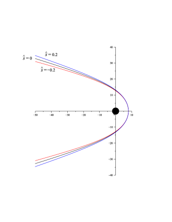
Figure 1: The hyperbolic-like orbits of a spinning test particle with $\hat{s}=\pm 0.2$ are shown in the $r$-$\phi$ plane for the choice of parameters $p=20$ and $e=1.5$ in comparison with the geodesic of a spinless particle ($\hat{s}=0$). The values of both energy and angular momentum per unit mass are different depending on $\hat{s}$, whereas the minimum approach distance $r_{\rm(per)}=8M$ is the same for all cases. The deflection angle is $\delta\approx 2.59122$ (i.e., $148.46608$ deg) for $\hat{s}=0$, $\delta\approx 2.65601$ (i.e., $152.17820$ deg) for $\hat{s}=-0.2$, and $\delta\approx 2.52643$ (i.e., $144.75397$ deg) for $\hat{s}=0.2$.

3.1 Periastron shift

A different (equivalent) parametrization of the orbit can be adopted in terms of energy $\hat{E}$ and angular momentum $\hat{J}$ instead of $p$ and $e$. In this case the periastron distance depends on $\hat{s}$, and can be determined from the turning points for radial motion. The equation of the orbit can be written as follows in terms of the dimensionless inverse radial variable $u=M/r$

$$\left(\frac{du}{d\phi}\right)^{2} = \frac{2}{\hat{J}}({\hat{J}}-{\hat{E}}{\hat{s}})\left[u^{3}-\frac{1}{2\hat{J}}({\hat{J}}+{\hat{E}}{\hat{s}})u^{2}+\frac{1}{{\hat{J}}^{3}}({\hat{J}}+3{\hat{E}}{\hat{s}})u\right.$$ (31)

$$\left.+\frac{1}{2{\hat{J}}^{3}}({\hat{E}}^{2}-1)({\hat{J}}+3{\hat{E}}{\hat{s}})\right]$$

$$\equiv \frac{2}{\hat{J}}({\hat{J}}-{\hat{E}}{\hat{s}})(u-u_{1})(u-u_{2})(u-u_{3})\,.$$

For hyperbolic orbits we have $u_{1}<0<u\leq u_{2}<u_{3}$, with $u_{2}$ corresponding to the closest approach distance, i.e., $r_{\rm(per)}=M/u_{2}$ Chandrasekhar:1985kt . In the geodesic case ($\hat{s}=0$) these roots are given by

$$u_{1\,(0)} = \frac{1}{6}\left[1-e^{-i\pi/3}X-e^{i\pi/3}\left(1-\frac{12}{{\hat{J}}^{2}}\right)\frac{1}{X}\right]\,,$$

$$u_{2\,(0)} = \frac{1}{6}\left[1-e^{i\pi/3}X-e^{-i\pi/3}\left(1-\frac{12}{{\hat{J}}^{2}}\right)\frac{1}{X}\right]\,,$$

$$u_{3\,(0)} = \frac{1}{6}\left[1+X+\left(1-\frac{12}{{\hat{J}}^{2}}\right)\frac{1}{X}\right]\,,$$ (32)

where

$$X=\frac{1}{\hat{J}}\left[\hat{J}\left({\hat{J}}^{2}-54{\hat{E}}^{2}+36\right)+6i\sqrt{3}\sqrt{\Delta_{(0)}}\right]^{1/3}\,,$$ (33)

When the discriminant

$$\Delta_{(0)}=({\hat{E}}^{2}-1){\hat{J}}^{4}-(27{\hat{E}}^{4}-36{\hat{E}}^{2}+8){\hat{J}}^{2}-16$$ (34)

is positive, the roots are all real, which is the case under consideration here. To first-order in spin, the corrections to the geodesic values are

$$u_{1} = u_{1\,(0)}-\frac{\hat{E}}{2{\hat{J}}^{3}}\frac{3({\hat{E}}^{2}-1)+u_{1\,(0)}(6-u_{1\,(0)}{\hat{J}}^{2})}{(u_{1\,(0)}-u_{3\,(0)})(u_{1\,(0)}-u_{2\,(0)})}\hat{s}\,,$$

$$u_{2} = u_{2\,(0)}-\frac{\hat{E}}{2{\hat{J}}^{3}}\frac{3({\hat{E}}^{2}-1)+u_{2\,(0)}(6-u_{2\,(0)}{\hat{J}}^{2})}{(u_{2\,(0)}-u_{1\,(0)})(u_{2\,(0)}-u_{3\,(0)})}\hat{s}\,,$$

$$u_{3} = u_{3\,(0)}-\frac{\hat{E}}{2{\hat{J}}^{3}}\frac{3({\hat{E}}^{2}-1)+u_{3\,(0)}(6-u_{3\,(0)}{\hat{J}}^{2})}{(u_{3\,(0)}-u_{1\,(0)})(u_{3\,(0)}-u_{2\,(0)})}\hat{s}\,,$$ (35)

satisfying the properties

$$u_{1}+u_{2}+u_{3}=\frac{1}{2}\left(1+\frac{\hat{E}}{\hat{J}}\hat{s}\right)\,.$$ (36)

Note that $u_{2}$ and $u_{3}$ can be obtained from $u_{1}$ simply by replacing indices cyclically. Eq. (31) then yields

$$\frac{d\phi}{du}=\pm\frac{1}{\sqrt{2}}\left(1+\frac{{\hat{E}}}{2\hat{J}}{\hat{s}}\right)\frac{1}{\sqrt{(u-u_{1})(u_{2}-u)(u_{3}-u)}}\,,$$ (37)

where the $\pm$ sign should be chosen properly during the whole scattering process, depending on the choice of initial conditions. For instance, by choosing $\phi(u_{2})=0$ at periastron, integration between $u_{2}$ and $u$ gives

$$\phi(u)=\mp\frac{\sqrt{2}}{\sqrt{u_{3}-u_{1}}}\left(1+\frac{{\hat{E}}}{2\hat{J}}{\hat{s}}\right)\left[K(m)-F(\alpha(u),m)\right]\,,$$ (38)

where

$$m=\sqrt{\frac{u_{2}-u_{1}}{u_{3}-u_{1}}}\,,\qquad\alpha(u)=\sqrt{\frac{u-u_{1}}{u_{2}-u_{1}}}\,.$$ (39)

The deflection angle is then

$$\delta(\hat{E},\hat{J},\hat{s}) = \frac{2\sqrt{2}}{\sqrt{u_{3}-u_{1}}}\left(1+\frac{{\hat{E}}}{2\hat{J}}{\hat{s}}\right)\left[K(m)-F(\alpha(0),m)\right]-\pi\,.$$ (40)

A typical orbit using this parametrization is shown in Fig. 2 (a). The two branches (upper $+$, lower $-$) join at the periastron on the horizontal axis. In Fig. 2 (b), instead, initial conditions are such that all trajectories start from a common spacetime point far from the hole ($u=0$, $\phi(0)=\phi_{-}$), and complete their scattering process with different minimum approach distances $r_{\rm(per)}=M/u_{2}$ at $\phi=\phi(u_{2})$ depending on the value of the spin parameter.

$$\begin{array}[]{cc}\includegraphics[scale={0.3}]{fig2a.eps}&\includegraphics[scale={0.3}]{fig2b.eps}\\ (a)&(b)\\ \end{array}$$

Figure 2: The hyperbolic-like orbits of a spinning test particle with $\hat{s}=\pm 0.2$ are shown in the $r$-$\phi$ plane for the choice of parameters $\hat{E}\approx 1.03334$ and $\hat{J}\approx 5.20756$ for two different sets of initial conditions. The reference geodesic is the same as in Fig. 1. In panel (a) the orbital equation (37) has been integrated starting from the periastron $r_{\rm(per)}=M/u_{2}$ located at $\phi(u_{2})=0$ for every value of $\hat{s}$. The deflection angle is $\delta\approx 2.59122$ (i.e., $148.46608$ deg) for $\hat{s}=0$, $\delta\approx 2.45760$ (i.e., $140.80996$ deg) for $\hat{s}=-0.2$, and $\delta\approx 2.70531$ (i.e., $155.00262$ deg) for $\hat{s}=0.2$. In panel (b), instead, the initial conditions have been chosen in such a way that all trajectories start from a common spacetime point far from the hole ($u=0$, $\phi(0)\approx-2.86621$). The periastron is at $u_{2}\approx 0.11520$ (i.e., $r_{\rm(per)}\approx 8.68044M$) and $\phi(u_{2})\approx-0.06687$ for $\hat{s}=-0.2$, $u_{2}=0.125$ (i.e., $r_{\rm(per)}=8M$) and $\phi(u_{2})=0$ for $\hat{s}=0$ and $u_{2}\approx 0.13400$ (i.e., $r_{\rm(per)}\approx 7.46247M$) and $\phi(u_{2})\approx 0.05704$ for $\hat{s}=0.2$.

3.2 Capture cross section

The condition for capture by the black hole is $u_{2}=u_{3}$, i.e., the cubic at the right hand side of Eq. (31) has a double root, corresponding to the vanishing of the discriminant Metner:1963 ; Misner:1974qy ; Collins:1973xf . Solving for $\hat{J}$ then yields the critical value of the dimensionless angular momentum for capture

$${\hat{J}}_{\rm crit}^{2}={\hat{J}}_{\rm crit\,(0)}^{2}\left[1+\frac{2\hat{s}}{{\hat{J}}_{\rm crit\,(0)}\hat{E}(9{\hat{E}}^{2}-8)}\left(3{\hat{E}}^{2}-2-\frac{8}{{\hat{J}}_{\rm crit\,(0)}^{2}}\right)\right]\,,$$ (41)

where

$${\hat{J}}_{\rm crit\,(0)}^{2}=\frac{27{\hat{E}}^{4}-36{\hat{E}}^{2}+8+{\hat{E}}(9{\hat{E}}^{2}-8)^{3/2}}{2{\hat{E}}^{2}-1}\,.$$ (42)

The associated cross section is thus given by

$$\sigma_{\rm capt}=\pi b_{\rm crit}^{2}\,,\qquad b_{\rm crit}=M\frac{{\hat{J}}_{\rm crit}}{\sqrt{{\hat{E}}^{2}-1}}\,,$$ (43)

where $b_{\rm crit}$ is the critical impact parameter. In the ultrarelativistic limit ($\hat{E}\gg 1$) the first order correction in spin to the capture cross section is thus given by

$$\sigma_{\rm capt}\big{|}_{\rm u.r.}=27\pi M^{2}\left[1+\frac{2}{3\hat{E}^{2}}\left(1+\frac{\sqrt{3}}{9}\hat{s}\right)+O\left(\frac{1}{\hat{E}^{4}}\right)\right]\,,$$ (44)

whereas for low energies ($\beta^{2}\equiv E^{2}-1\ll 1$)

$$\sigma_{\rm capt}\big{|}_{\rm n.r.}=16\pi M^{2}\frac{1}{\beta^{2}}\left(1+\frac{1}{4}\hat{s}\right)+O(\beta^{0})\,.$$ (45)

4 Discussion

Most of the existing studies on spinning particle motion in a Schwarzschild spacetime concern either circular or eccentric orbits or even deviations due to spin from a reference orbit which is a circular geodesic (i.e., quasi-circular orbits) Rietdijk:1992tx ; Apostolatos:1996 ; Bini:2004md ; Bini:2005nt ; Plyatsko:2005bh ; Mohseni:2010rm ; Bini:2014poa ; Plyatsko:2011wp ; Costa:2012cy ; Harms:2016ctx . These results are useful when taking into account backreaction effects to the background metric, going beyond the test particle approximation by using, e.g., self-force techniques Sasaki:2003xr . Furthermore, it has been shown in Ref. Burko:2003rv that the conservative effect on the orbital dynamics in the extreme mass ratio limit is typically dominated by the spin force (with respect to the conservative part of the local self-force), whereas the decay of the orbit is dominated by radiation reaction. As a consequence, in the construction of the gravitational waveforms the contribution of the spin-orbit coupling may be much more important for astrophysical systems than that due to the self-force.

We have considered here hyperbolic-like orbits, extending previous results. The analytical solution of the orbit as well as observational effects like the correction due to spin to the scattering angle and the shift of the periastron may be useful for modeling spin effects in scattering processes in the framework of perturbation theory. We briefly discuss below some reciprocity relations concerning the companion problem of a particle without structure moving along a hyperbolic-like geodesic in a slowly rotating Kerr spacetime. Finally, we compare the effects due to the spin force with those of a drag force studied elsewhere.

4.1 Comparison with the hyperbolic-like geodesic motion in a slowly rotating Kerr spacetime

One can compare Eq. (22) governing the evolution of $\phi$ as a function of $\chi$ during the scattering process in the case of spinning particle orbiting a Schwarzschild black hole (in the small spin approximation) with the analogous equation valid for a spinless particle moving along a hyperbolic-like geodesic orbit in a Kerr spacetime (in the approximation of small rotation).

To first-order in the rotation parameter $\hat{a}=a/M$ the dimensionless energy and angular momentum are given by

$$\hat{E} = \hat{E}_{0}-\hat{a}\frac{(1-e^{2})^{2}}{p(p-3-e^{2})^{3/2}}\,,$$

$$\hat{J} = \hat{J}_{0}-\hat{a}\frac{(3+e^{2})\sqrt{(p-2)^{2}-4e^{2}}}{p^{1/2}(p-3-e^{2})^{3/2}}\,,$$ (46)

whereas the orbital equation reads

$$\frac{d\phi}{d\chi}\Big{|}_{\rm kerr,\,geo} = \frac{1}{\sqrt{1-6u_{p}-2eu_{p}\cos\chi}}$$

$$- 4\hat{a}\frac{\hat{E}_{0}u_{p}}{\hat{J}_{0}}\frac{1}{(1-6u_{p}-2eu_{p}\cos\chi)^{3/2}(1-2u_{p}-2eu_{p}\cos\chi)}\,.$$

In the weak field limit (i.e., $u_{p}\ll 1$) the two equations of the orbit of a spinless (geodesic) particle in a Kerr background and a spinning particle in a Schwarzschild spacetime become

$$\frac{d\phi}{d\chi}\Big{|}_{\rm kerr,\,geo}-\frac{d\phi}{d\chi}\Big{|}_{\rm schw,\,geo} = -4\hat{a}u_{p}^{3/2}+O(u_{p}^{5/2})\,,$$

$$\frac{d\phi}{d\chi}\Big{|}_{\rm schw,\,spin}-\frac{d\phi}{d\chi}\Big{|}_{\rm schw,\,geo} = -(3+e\cos\chi)\hat{s}u_{p}^{3/2}+O(u_{p}^{5/2})\,,$$ (48)

respectively, where

$$\frac{d\phi}{d\chi}\Big{|}_{\rm schw,\,geo}=1+(e\cos\chi+3)u_{p}+\frac{3}{2}(e\cos\chi+3)^{2}u_{p}^{2}+O(u_{p}^{3})\,.$$ (49)

It then follows that to the leading order in $u_{p}$ (i.e., neglecting also corrections due to eccentricity) the two equations are mapped one into the other simply by replacing $3\hat{s}\to 4\hat{a}$, or equivalently

$$\frac{3}{2}\hat{s}\quad\to\quad 2\hat{a}\,.$$ (50)

Let us denote by $m_{1}=m$ and $S_{1}=s$ the mass and spin of the particle and by $m_{2}=M$ ($m_{1}\ll m_{2}$) and $S_{2}=m_{2}a$ those of the black hole. Restoring then the mass factors, i.e., $\hat{s}={S_{1}}/{m_{1}m_{2}}$ and $\hat{a}=S_{2}/m_{2}^{2}$, the above relation becomes

$$\frac{3}{2}\frac{S_{1}}{m_{1}m_{2}}\quad\to\quad 2\frac{S_{2}}{m_{2}^{2}}\,,$$ (51)

that is

$$\frac{3}{2}\frac{m_{2}}{m_{1}}S_{1}\quad\to\quad 2S_{2}\,.$$ (52)

In the discussion of a two-body systems with spins Damour:2007nc , two new spin variables are known to play a role, namely

$$S_{*}=\frac{m_{2}}{m_{1}}S_{1}+\frac{m_{1}}{m_{2}}S_{2}\,,\qquad S=S_{1}+S_{2}\,.$$ (53)

Here, from the Schwarzschild point of view $S_{2}=0$ and the only surviving spin variable is $S_{*}=(m_{2}/m_{1})S_{1}$. Similarly, from the Kerr point of view (where the considered particle is spinless and moves along a geodesic) the only surviving spin variable is $S=S_{2}$. This means that Eq. (52) can be cast in the form

$$\frac{3}{2}S_{*}\quad\to\quad 2S\,,$$ (54)

in the approximation specified above in which these considerations hold. It is now easy to recognize the gyrogravitomagnetic ratios introduced in Ref. Damour:1992qi , i.e.,

$$g_{S_{*}}=\frac{3}{2}\,,\qquad g_{S}=2\,,$$ (55)

at their leading order values. Finally, Eq. (52) becomes

$$g_{S_{*}}S_{*}\quad\to\quad g_{S}S\,,$$ (56)

as expected.

4.2 Comparison of effects due to the spin force with those of a drag force

In a recent work Bini:2016ubc we have investigated the situation in which the particles under consideration were (structureless) test particles, whose deviation from geodesic motion was due to an (external) drag force $F_{\rm(drag)}$, chosen so that its components in the plane of motion are proportional to the corresponding components of the $4$-velocity itself, i.e., $F_{\rm(drag)}^{r}\propto U^{r}$ and $F_{\rm(drag)}^{\phi}\propto U^{\phi}$, namely

$$F_{\rm(drag)}=F_{\rm(drag)}^{t}\partial_{t}-\lambda\left(U^{r}\partial_{r}+U^{\phi}\partial_{\phi}\right)\,,$$ (57)

with $\lambda$ a dimensionless constant modeling the physics of the dragging. This is the case of particles interacting with accreting flows also in the presence of external electromagnetic fields or plasma McCourt:2015dpa . The temporal component follows from the orthogonality condition of $F_{\rm(drag)}$ and $U$, i.e., $F_{\rm(drag)}\cdot U=0$, leading to

$$F_{\rm(drag)}=-\lambda\gamma\left\{\left[(\nu^{\hat{r}})^{2}+(\nu^{\hat{\phi}})^{2}\right]n+\nu^{\hat{r}}e_{\hat{r}}+\nu^{\hat{\phi}}e_{\hat{\phi}}\right\}\,.$$ (58)

This drag force acts on the orbital plane like a viscous force, so that is has dissipative effects, leading to the loss of energy and angular momentum during the scattering process. In contrast, the spin force (12) acts as a conservative force, the total energy and angular momentum being constants of motion, implying that the scattering process is perfectly symmetric with respect to the minimum approach distance, as we have shown above. In both cases, as a common feature particles are either scattered or captured by the black hole.

There also exist other kinds of dragging, like that leading to the well known Poynting-Robertson effect PR , where the presence of a superposed photon test field implies the existence of a critical radius at which the radiation pressure balances the gravitational attraction, allowing rings of matter to form (see, e.g., Refs. abram ; ML ; Bini:2008vk ; Bini:2011zza ; Bini:2014yca for recent applications to different backgrounds of astrophysical interest). The interplay between spin and radiation forces has been discussed in Ref. Bini:2010xa by analyzing the deviation from circular geodesic motion. A temporal counterpart to the Poynting-Robertson effect has been considered very recently in Ref. Bini:2016tqz , where a distribution of collisionless dust around the black hole is responsible for the drag instead of the radiation field. In both cases the friction force has the form

$$F_{\rm(drag)}^{\alpha}=-\sigma P(U)^{\alpha}{}_{\mu}T^{\mu\nu}U_{\nu}\,,$$ (59)

where $P(U)$ projects orthogonally to $U$ and $\sigma$ denotes the (constant) effective interaction cross section, built with either the stress-energy tensor $T^{\mu\nu}=T_{\rm(rad)}^{\mu\nu}$ associated with the photon field or that $T^{\mu\nu}=T_{\rm(dust)}^{\mu\nu}$ associated with the dust field. The existence of equilibrium orbits may prevent particles moving on a scattering orbit from either falling into the hole or escaping to infinity.

In future works we will extend the above discussion to the more interesting situation of a Kerr spacetime, where the rotation of the hole plays an important role.

- (1) B. P. Abbott et al. [LIGO Scientific and Virgo Collaborations], “Observation of Gravitational Waves from a Binary Black Hole Merger,” Phys. Rev. Lett. 116, 061102 (2016) [arXiv:1602.03837 [gr-qc]].
- (2) R. Ruffini, J.A. Wheeler, “Gravitational Radiation,” in The astrophysical aspects of the weak interactions, Cortona 1970, ed. by G. Bernardini, E. Amaldi, and L. Radicati, ANL Quaderno n. 157, p. 165 (Accademia Nazionale dei Lincei, Roma, 1971).
- (3) M. Rees, R. Ruffini and J. A. Wheeler, “Black Holes, Gravitational Waves and Cosmology: An Introduction to Current Research,” Topics in Astrophysics and Space Physics, vol. 10 (Gordon and Breach, Science Publishers, Inc., New York, 1974).
- (4) L. Blanchet and G. Schaefer, “Higher order gravitational radiation losses in binary systems,” Mon. Not. Roy. Astron. Soc. 239, 845 (1989) Erratum: [Mon. Not. Roy. Astron. Soc. 242, 704 (1990)].
- (5) F. Pretorius and D. Khurana, “Black hole mergers and unstable circular orbits,” Class. Quant. Grav. 24, S83 (2007) [gr-qc/0702084].
- (6) M. Shibata, H. Okawa and T. Yamamoto, “High-velocity collision of two black holes,” Phys. Rev. D 78, 101501 (2008) [arXiv:0810.4735 [gr-qc]].
- (7) U. Sperhake, V. Cardoso, F. Pretorius, E. Berti and J. A. Gonzalez, “The High-energy collision of two black holes,” Phys. Rev. Lett. 101, 161101 (2008) [arXiv:0806.1738 [gr-qc]].
- (8) U. Sperhake, V. Cardoso, F. Pretorius, E. Berti, T. Hinderer and N. Yunes, “Cross section, final spin and zoom-whirl behavior in high-energy black hole collisions,” Phys. Rev. Lett. 103, 131102 (2009) [arXiv:0907.1252 [gr-qc]].
- (9) U. Sperhake, E. Berti, V. Cardoso and F. Pretorius, “Universality, maximum radiation and absorption in high-energy collisions of black holes with spin,” Phys. Rev. Lett. 111, 041101 (2013) [arXiv:1211.6114 [gr-qc]].
- (10) J. Majar, P. Forgacs and M. Vasuth, “Gravitational waves from binaries on unbound orbits,” Phys. Rev. D 82, 064041 (2010) [arXiv:1009.5042 [gr-qc]].
- (11) D. Bini and T. Damour, “Gravitational radiation reaction along general orbits in the effective one-body formalism,” Phys. Rev. D 86, 124012 (2012) [arXiv:1210.2834 [gr-qc]].
- (12) T. Damour, F. Guercilena, I. Hinder, S. Hopper, A. Nagar and L. Rezzolla, “Strong-Field Scattering of Two Black Holes: Numerics Versus Analytics,” Phys. Rev. D 89, 081503 (2014) [arXiv:1402.7307 [gr-qc]].
- (13) L. De Vittori, A. Gopakumar, A. Gupta and P. Jetzer, “Gravitational waves from spinning compact binaries in hyperbolic orbits,” Phys. Rev. D 90, 124066 (2014) [arXiv:1410.6311 [gr-qc]].
- (14) M. Mathisson, “Neue mechanik materieller systemes,” Acta Phys. Polon. 6, 163 (1937).
- (15) A. Papapetrou, “Spinning test particles in general relativity. 1.,” Proc. Roy. Soc. Lond. A 209, 248 (1951).
- (16) W. G. Dixon, “Dynamics of extended bodies in general relativity. I. Momentum and angular momentum,” Proc. Roy. Soc. Lond. A 314, 499 (1970).
- (17) W. Tulczyjew, “Motion of multipole particles in general relativity theory,” Acta Phys. Polon. 18, 393 (1959).
- (18) S. Chandrasekhar, “The mathematical theory of black holes,” Clarendon, Oxford, UK, 1985.
- (19) A. W. K. Metzner, “ Observable Properties of Large Relativistic Masses,” Journal of Mathematical Physics 4, 1194 (1963).
- (20) C. W. Misner, K. S. Thorne and J. A. Wheeler, “Gravitation,” Freeman, San Francisco, 1973.
- (21) P. A. Collins, R. Delbourgo and R. M. Williams, “On the elastic Schwarzschild scattering cross-section,” J. Phys. A 6, 161 (1973).
- (22) R. H. Rietdijk and J. W. van Holten, “Spinning particles in Schwarzschild space-time,” Class. Quant. Grav. 10, 575 (1993).
- (23) T. A. Apostolatos, “A spinning test body in the strong field of a Schwarzschild black hole,” Class. Quant. Grav. 13, 799 (1996).
- (24) D. Bini, F. de Felice and A. Geralico, “Spinning test particles and clock effect in Schwarzschild spacetime,” Class. Quant. Grav. 21, 5427 (2004) [gr-qc/0410082].
- (25) D. Bini, F. de Felice, A. Geralico and R. T. Jantzen, “Spin precession in the Schwarzschild spacetime: Circular orbits,” Class. Quant. Grav. 22, 2947 (2005) [gr-qc/0506017].
- (26) R. Plyatsko, “Ultrarelativistic circular orbits of spinning particles in a Schwarzschild field,” Class. Quant. Grav. 22, 1545 (2005) [gr-qc/0507023].
- (27) M. Mohseni, “Stability of circular orbits of spinning particles in Schwarzschild-like space-times,” Gen. Rel. Grav. 42, 2477 (2010) [arXiv:1005.3110 [gr-qc]].
- (28) D. Bini, A. Geralico and R. T. Jantzen, “Spin-geodesic deviations in the Schwarzschild spacetime,” Gen. Rel. Grav. 43, 959 (2011) [arXiv:1408.4946 [gr-qc]].
- (29) R. M. Plyatsko and M. T. Fenyk, “Highly relativistic spinning particle in the Schwarzschild field: Circular and other orbits,” Phys. Rev. D 85, 104023 (2012) [arXiv:1111.0804 [gr-qc]].
- (30) L. F. O. Costa, J. Natário and M. Zilhao, “Spacetime dynamics of spinning particles: Exact electromagnetic analogies,” Phys. Rev. D 93, no. 10, 104006 (2016) [arXiv:1207.0470 [gr-qc]].
- (31) E. Harms, G. Lukes-Gerakopoulos, S. Bernuzzi and A. Nagar, “Spinning test body orbiting around a Schwarzschild black hole: Circular dynamics and gravitational-wave fluxes,” Phys. Rev. D 94, no. 10, 104010 (2016) [arXiv:1609.00356 [gr-qc]].
- (32) M. Sasaki and H. Tagoshi, “Analytic black hole perturbation approach to gravitational radiation,” Living Rev. Rel. 6, 6 (2003) [gr-qc/0306120].
- (33) L. M. Burko, “Orbital evolution of a particle around a black hole. 2. Comparison of contributions of spin orbit coupling and the self-force,” Phys. Rev. D 69, 044011 (2004) [gr-qc/0308003].
- (34) T. Damour, P. Jaranowski and G. Schaefer, “Hamiltonian of two spinning compact bodies with next-to-leading order gravitational spin-orbit coupling,” Phys. Rev. D 77, 064032 (2008) [arXiv:0711.1048 [gr-qc]].
- (35) T. Damour, M. Soffel and C. m. Xu, “General relativistic celestial mechanics. 3. Rotational equations of motion,” Phys. Rev. D 47, 3124 (1993).
- (36) D. Bini and A. Geralico, “Scattering by a Schwarzschild black hole of particles undergoing drag force effects,” Gen. Rel. Grav. 48, 101 (2016).
- (37) M. McCourt and A. M. Madigan, “Going with the flow: using gas clouds to probe the accretion flow feeding Sgr A*,” Mon. Not. Roy. Astron. Soc. 455, 2187 (2016). [arXiv:1503.04801 [astro-ph.HE]].
- (38) J. H. Poynting, “Radiation in the Solar System: Its Effect on Temperature and Its Pressure on Small Bodies,” Phil. Trans. Roy. Soc. 202, 525 (1904); H. P. Robertson, “Dynamical effects of radiation in the solar system,” Mon. Not. Roy. Astron. Soc. 97, 423 (1937).
- (39) M. A. Abramowicz, G. F. R. Ellis, and A. Lanza, “Relativistic effects in superluminal jets and neutron star winds,” Astrophys. J. 361, 470 (1990)
- (40) M. C. Miller and F. K. Lamb, “Motion of Accreting Matter near Luminous Slowly Rotating Relativistic Stars,” Astrophys. J. 470, 1033 (1996)
- (41) D. Bini, R. T. Jantzen and L. Stella, “The General relativistic Poynting-Robertson effect,” Class. Quant. Grav. 26, 055009 (2009) [arXiv:0808.1083 [gr-qc]].
- (42) D. Bini, A. Geralico, R. T. Jantzen, O. Semeràk and L. Stella, “The general relativistic Poynting-Robertson effect: II. A photon flux with nonzero angular momentum,” Class. Quant. Grav. 28, 035008 (2011) [arXiv:1408.4945 [gr-qc]].
- (43) D. Bini, A. Geralico and A. Passamonti, “Radiation drag in the field of a non-spherical source,” Mon. Not. Roy. Astron. Soc. 446, 65 (2015) [arXiv:1410.3099 [astro-ph.HE]].
- (44) D. Bini and A. Geralico, “Spinning bodies and the Poynting-Robertson effect in the Schwarzschild spacetime,” Class. Quant. Grav. 27, 185014 (2010) [arXiv:1107.2793 [gr-qc]].
- (45) D. Bini and A. Geralico, “Schwarzschild black hole embedded in a dust field: scattering of particles and drag force effects,” Class. Quant. Grav. 33, 125024 (2016).