Implications of Realistic Fracture Criteria on Crack Morphology

Abstract

We study the effects realistic fracture criteria have on crack morphology obtained in numerical simulations with a stochastic discrete element method. Results are obtained with two criteria which are consistent with the theory of elasticity and compared with previous results using the original criterion, chosen when the method was first published. The conventional choice has been to consider the combined loading as an interaction between bending and tensile forces only, leaving out shear forces altogether. Moreover the combination of bending and tension used in the old criterion is correct only for plastic deformations. Our results show that the inclusion of shear forces have a profound effect on crack morphology. We consider two types of external loading, torsion applied to a circular cylinder and tension applied to a cube. In the tensile case, the exponent which characterises scaling of crack roughness with system size is found to be very close to the experimental value $\zeta\sim 0.5$ when realistic fracture criteria are used. In the present calculations we obtain $\zeta=0.52$, a value which remains constant for all disorders. It is proposed that the small-scale exponent $\zeta=0.8$ appears as a consequence of cleavage between crystal planes and consequently requires a different fracture criterion than that which is used on larger scales.

I Introduction

Material properties have long been studied using finite element methods. A different approach to fracture and breakdown phenomena was introduced almost three decades ago within the statistical physics community. In this approach, a macroscopic material is though to be made up of discrete elements arranged on a lattice or grid. Into this discretized version of the material random variations in structural properties are introduced at the scale of the discrete elements. This can be done for the elastic properties of the elements or, as is more common, it can be made to affect the individual breaking strengths of the elements. The resulting breakdown process, whether it takes the form of electrical failure in a network of fuses or describes the elastic breaking of a discretized continuum, is complex and results in a rough crack interface.

In stochastic discrete element modeling of elastic media there have been mainly two ways to model forces within the continuum, i.e., in terms of ’springs’ born or in terms of ’beams’ roux ; herr . The former approach is simpler and less requiring of computational resources since in this case bending and shear forces are absent on the level of the individual element (the spring). The latter approach is more realistic since it reproduces the full mechanical response of a real solid, i.e., each ’beam’ transmits axial forces, bending moments, transverse shear and torsion to its adjoining neighbours.

One popular quantity to study has been crack morphology as quantified by the roughness exponent. This can be measured experimentally and is therefore an important quantity to be reproduced by the theoretical models available. The typically rough crack surface that is obtained in materials with a heterogeneous microstructure is due to a complex interplay between stresses and local variations in material structure. Such variations can be due to a granular structure with different grain sizes, with the grains being randomly distributed and subject to different bonding strengths. Material disorder can be due to a fibrous structure, or a structure characterized by pores and voids, or it can be dominated by the presence of microscopic cracks, inclusions and fault lines. Strength variations may be in the form of weak spots in the material or local regions that are stronger than the surroundings.

If we consider fracture in such disordered media, this is a coupled process whereby stresses evolve according to how cracks grow while cracks develop according to how stresses are distributed. At some point the fracture process goes from being disorder dominated, where new cracks appear randomly, to being stress dominated, where smaller cracks merge into a large crack. In this coupled process a path is now forged through the medium by the moving front of this crack. The fracture criterion plays an important role in determining the exact nature of the path taken. In other words, its role is to decide the outcome of the interplay between stress and disorder. It is therefore extremely important to study how different fracture criteria influence the fracturing process. As we shall see the role played by the fracture criterion is also affected by, and intimately associated with, lattice morphology. A criterion which does not allow for failure in transverse loading will display a tendency towards fracturing along lattice planes.

In simple stochastic models of fracture, such as the random fuse model, there isn’t much choice as far as the fracture criterion is concerned. Here the ratio of the current which flows through an element to the burn-out threshold of that element is what constitutes the breaking criterion. There really is no other choice. In elastic fracture, on the other hand, there are several modes of loading and each of these can contribute to the breaking of an element. This is especially so whenever forces are defined in terms of ’beams’. In the case of ’springs’ only axial forces exist on the scale of the individual element. When the full elastic response is included, however, an element breaks if the axial load exceeds a certain limit or if the shear exceeds a certain limit. In general the situation is a combined loading.

Much effort has been expended within engineering communities to obtain simplified, yet realistic, interaction formulae relevant to various loading conditions. Typically, the nature of these fracture criteria depend on the type of material used, the shape or cross section of the element involved, and the specific application concerned. They can be theoretically derived or empirically deduced from laboratory tests, or they can be based on a combination of approaches.

Stochastic fracture models were developed within the statistical physics community and consequently much interest has been focused on the complex process of interaction between stress and disorder. This is probably one reason why failure criteria have received less attention than what would have been the case within the engineering community.

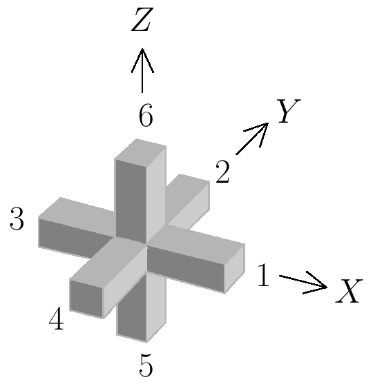
Figure 1: Enumeration scheme for the discrete ’beam’ elements of a cube lattice connecting node $i$ to its nearest neighbours $j=1$ to $j=6$, showing the coordinate system with node $i$ as its origin.

II Discrete Element Model

Our model is a deformable lattice in the form of a regular cube with size $L\times L\times L$, where each node is connected to its nearest neighbours by linearly elastic beams. Forces acting on the nodes have been deduced from the effect a concentrated end-load has on a beam with no end-restraints roar ; cran . A coordinate system is placed on each node, and the enumeration of the connecting beams follows an anti-clockwise scheme within the $XY$-plane, i.e., beginning with the beam which lies along the positive $X$-axis and ending with that which extends upwards along the positive $Z$-axis, see Fig. 1.

At each stage of the breaking process, the updated displacements for each node is obtained from

$$\sum_{j}{\bf D}_{ij}\left[\begin{array}[]{l}x_{i}\\ y_{i}\\ z_{i}\\ u_{i}\\ v_{i}\\ w_{i}\\ \end{array}\right]=\lambda\left[\begin{array}[]{l}X_{i}\\ Y_{i}\\ Z_{i}\\ U_{i}\\ V_{i}\\ W_{i}\\ \end{array}\right],$$ (13)

which is solved iteratively via relaxation using the conjugate gradient method hest ; teuk . This minimizes the elastic energy to obtain those displacements for which the sum of forces and moments on each node vanish, i.e. the mechanical equilibrium. In Eq. (13), $x_{i}$, $y_{i}$ and $z_{i}$ are the coordinate displacements of node $i$ relative to its starting position before fracturing is initiated. Likewise, $u_{i}$, $v_{i}$ and $w_{i}$ are the angular displacements around the $X$-, $Y$- and $Z$-axes, respectively (see Fig. 1).

Presently we use the same expressions for force and moment as those used in Refs. herr and skje . We thus have three constants

$$\alpha=\frac{\ell}{EA},\qquad\beta=\frac{\ell}{GA},\qquad\gamma=\frac{\ell^{3}}{EI},$$ (14)

where $E$ and $G$ are Young’s modulus and the shear modulus, respectively, $A$ is the area of the discrete element cross section, $\ell$ is its length and $I$ the moment of inertia about the centroidal axis. Our choice of these parameters mirrors that of Refs. herr and skje , i.e., the length is set to $\ell=1$ and we use $\alpha=1$, $\beta=30/7$ and $\gamma=60/7$. Additionally, we define the quantity

$$\rho=\frac{\ell}{JG},$$ (15)

where $J$ is the moment of inertia for torsion. Here we use $\rho=1$. In the following we define

$$\delta x_{j}\equiv x_{i}-x_{j},$$ (16)

and similarly for the other five coordinates.

Six terms contribute to each of the force components in Eq. (13). For instance, if we imagined the neighbouring nodes to be fixed, a translation $x_{i}$ of the central node $i$ would induce axial forces in beams $1$ and $3$ and transverse forces in beams $2$, $4$, $5$ and $6$. If we take into account the displacements of the neighbouring nodes as well, the axial force on node $i$ from beam $1$ is

$$A_{i}^{(1)}=-\frac{1}{\alpha}\delta x_{1},$$ (17)

while the transverse force on node $i$ from beam $2$, along the $X$-axis, is given by

$${{}_{x}}S_{i}^{(2)}=-\frac{1}{\beta+\frac{\gamma}{12}}\Bigl{[}\delta x_{2}-\frac{1}{2}\bigl{(}w_{i}+w_{j}\bigr{)}\Bigr{]}.$$ (18)

In each case $j$ refers to the neighbour depicted in Fig. 1. Consequently,

$$X_{i}=A_{i}^{(1)}+A_{i}^{(3)}+\sum_{j\neq 1,3}^{6}{{}_{x}}S_{i}^{(j)}$$ (19)

is how the force on node $i$ along the $X$-axis depends on the displacements and rotations of its six nearest neighbouring nodes. Similar expressions are deduced for $Y_{i}$ or $Z_{i}$ by considering translations along the $Y$-axis or the $Z$-axis, respectively.

An angular displacement $u_{i}$ about the $X$-axis with the neighbouring nodes fixed would create torque in beams $1$ and $3$, and bending in beams $2$, $4$, $5$ and $6$. More generally, the torque in node $i$ from beam $1$ is

$$T_{i}^{(1)}=-\frac{1}{\rho}\delta u_{1},$$ (20)

while the bending moment from beam $2$ is

$${{}_{u}}M_{i}^{(2)}=-\frac{1}{\beta+\frac{\gamma}{12}}\Bigl{[}\frac{\beta}{\gamma}\delta u_{2}+\frac{1}{2}\bigl{(}\delta z_{2}+\frac{2}{3}u_{i}+\frac{1}{3}u_{j}\bigr{)}\Bigr{]}.$$ (21)

For the angular force on node $i$ about the $X$-axis and its dependence on the displacements of the six neighbouring nodes, we have

$$U_{i}=T_{i}^{(1)}+T_{i}^{(3)}+\sum_{j\neq 1,3}^{6}{{}_{u}}M_{i}^{(j)},$$ (22)

now with similar expressions for $V_{i}$ and $W_{i}$.

To express the thirty-six force components in Eq. (13) more compactly,

$$r_{j}=\prod_{n=0}^{j-1}\bigl{(}-1\bigr{)}^{n}$$ (23)

and

$$s_{j}=\bigl{(}-1\bigr{)}^{j}r_{j}$$ (24)

are quantities which we define for notational convenience, to keep track of the signs and contributions from neighbouring beams. The $j$ in each case refers to the neighbouring beams as shown in Fig. 1. The Kronecker delta, moreover, has been used to construct

$$\widehat{\lambda}_{s,t}=\delta_{sj}+\delta_{tj},$$ (25)

i.e., an operator which includes $s$ and $t$ in the sum over neighbours (excluding the other four), and

$$\widehat{\chi}_{s,t}=\bigl{(}1-\delta_{sj}\bigr{)}\bigl{(}1-\delta_{tj}\bigr{)},$$ (26)

which instead excludes $s$ and $t$ from the sum over neighbours (including the other four).

For the six components making up the force on node $i$ along the $X$-axis, i.e., Eq. (19), we can now state this on a compact form as

$$X_{i}=-\frac{1}{\alpha}\sum_{j=1}^{6}\widehat{\lambda}_{1,3}\delta x_{j}-\frac{1}{\beta+\frac{\gamma}{12}}\sum_{j=1}^{6}\widehat{\chi}_{1,3}\biggl{\{}\delta x_{j}+\frac{r_{j}}{2}\Bigl{[}\widehat{\lambda}_{5,6}\bigl{(}v_{i}+v_{j}\bigr{)}+\widehat{\lambda}_{2,4}\bigl{(}w_{i}+w_{j}\bigr{)}\Bigr{]}\biggr{\}},$$ (27)

and $Y_{i}$ as

$$Y_{i}=-\frac{1}{\alpha}\sum_{j=1}^{6}\widehat{\lambda}_{2,4}\delta y_{j}-\frac{1}{\beta+\frac{\gamma}{12}}\sum_{j=1}^{6}\widehat{\chi}_{2,4}\biggl{\{}\delta y_{j}+\frac{r_{j}}{2}\Bigl{[}\widehat{\lambda}_{5,6}\bigl{(}u_{i}+u_{j}\bigr{)}+\widehat{\lambda}_{1,3}\bigl{(}w_{i}+w_{j}\bigr{)}\Bigr{]}\biggr{\}}.$$ (28)

In the same way, $Z_{i}$ becomes

$$Z_{i}=-\frac{1}{\alpha}\sum_{j=1}^{6}\widehat{\lambda}_{5,6}\delta z_{j}-\frac{1}{\beta+\frac{\gamma}{12}}\sum_{j=1}^{6}\widehat{\chi}_{5,6}\biggl{\{}\delta z_{j}-\frac{s_{j}}{2}\Bigl{[}\widehat{\lambda}_{2,4}\bigl{(}u_{i}+u_{j}\bigr{)}+\widehat{\lambda}_{1,3}\bigl{(}v_{i}+v_{j}\bigr{)}\Bigr{]}\biggr{\}},$$ (29)

Next, Eq. (22) for angular displacements about the $X$-axis is written out in full as

$$U_{i}=-\frac{1}{\rho}\sum_{j=1}^{6}\widehat{\lambda}_{1,3}\delta u_{j}-\frac{1}{\beta+\frac{\gamma}{12}}\sum_{j=1}^{6}\widehat{\chi}_{1,3}\biggl{\{}\frac{\beta}{\gamma}\delta u_{j}+\frac{r_{j}}{2}\Bigl{[}\hskip 1.42262pt\widehat{\lambda}_{5,6}\delta y_{j}-\widehat{\lambda}_{2,4}\delta z_{j}\Bigr{]}+\frac{1}{3}\bigl{(}u_{i}+\frac{1}{2}u_{j}\bigr{)}\biggr{\}},$$ (30)

and $V_{i}$, for angular displacements about the $Y$-axis, becomes

$$V_{i}=-\frac{1}{\rho}\sum_{j=1}^{6}\widehat{\lambda}_{2,4}\delta v_{j}-\frac{1}{\beta+\frac{\gamma}{12}}\sum_{j=1}^{6}\widehat{\chi}_{2,4}\biggl{\{}\frac{\beta}{\gamma}\delta v_{j}+\frac{r_{j}}{2}\Bigl{[}\hskip 1.42262pt\widehat{\lambda}_{5,6}\delta x_{j}-\widehat{\lambda}_{1,3}\delta z_{j}\Bigr{]}+\frac{1}{3}\bigl{(}v_{i}+\frac{1}{2}v_{j}\bigr{)}\biggr{\}}.$$ (31)

Lastly, for angular displacements about the $Z$-axis, we get

$$W_{i}=-\frac{1}{\rho}\sum_{j=1}^{6}\widehat{\lambda}_{5,6}\delta w_{j}-\frac{1}{\beta+\frac{\gamma}{12}}\sum_{j=1}^{6}\widehat{\chi}_{5,6}\biggl{\{}\frac{\beta}{\gamma}\delta w_{j}+\frac{r_{j}}{2}\Bigl{[}\hskip 1.42262pt\widehat{\lambda}_{2,4}\delta x_{j}+\widehat{\lambda}_{1,3}\delta y_{j}\Bigr{]}+\frac{1}{3}\bigl{(}w_{i}+\frac{1}{2}w_{j}\bigr{)}\biggr{\}}.$$ (32)

III Disorder

To include structural disorder we generate a random number $r$ on the unit interval $[0,1]$ and let this represent the cumulative threshold distribution. We assign thresholds according to $t_{\rm F}=r^{D}$, where $D>0$ is a power law with a maximum threshold of $1$ and a tail extending towards zero. The cumulative distribution function is then given by

$$P(t_{\rm F})=t_{\rm F}^{1/D},$$ (33)

where $0\leq t_{\rm F}\leq 1$. The case of $D=0$ corresponds to all thresholds being the same ($t_{\rm F}=1$), i.e., we have a homogeneous medium without structural disorder. An increase in the magnitude of the exponent $|D|$ causes the coefficient of variation with respect to any two random numbers $r$ and $r^{\prime}$ on the interval $[0,1]$ to increase. Therefore large values of $|D|$ correspond to strong disorders and small values to weak disorders.

IV Fracture Criteria

The original fracture criterion introduced by Herrmann et al. in Ref. herr considers a combination of bending and axial force, where beams fail when

$$\left(\frac{F}{t_{F}}\right)^{2}+\frac{|M|}{t_{M}}>1,$$ (34)

that is, using a squared term for the axial force and a linear term for the bending moment. The quantities $t_{\rm F}$ and $t_{\rm M}$ are thresholds for the amount of bending the element can support before failing. In applications other than stochastic modeling, there are two scenarios where this particular fracture criterion is frequently used. One is in connection with combined loadings for slender beams in compression stal . The other is for materials where plastic yielding occurs, in which case the loading can be either tensile or compressive chak . Presently we consider brittle fracture only.

Combined Axial Force and Bending

In wood constructions the region of safe loading for beam columns with rectangular cross sections, when subjected to a combination of axial tension and bending ndsw , is given as

$$\frac{F}{t_{F}}+\frac{M}{t_{M}}>1$$ (35)

in the unixial case, and

$$\frac{F}{t_{F}}+\frac{M_{x}}{t_{M_{x}}}+\frac{M_{y}}{t_{M_{y}}}>1$$ (36)

in the biaxial case, while the criterion for failure in compression is

$$\left(\frac{F}{t_{F}}\right)^{2}+\frac{M}{t_{M}}>1$$ (37)

in the uniaxial case, and

$$\left(\frac{F}{t_{F}}\right)^{2}+\frac{M_{x}}{t_{M_{x}}}+\frac{M_{y}}{t_{M_{y}}}>1$$ (38)

in the biaxial case. Deflection of the beam in the presence of a compressive force tends to magnify the moment that causes it, and consequently more emphasis is lent to the axial term. This distinction between tensile and compressive loading, however, is irrelevant to applications in the discrete element model. The reason is that the model is meant to describe a continuum rather than a physical lattice. In order to emulate the behaviour of a continuum, elements defining forces between nodes should not be considered to be slender. In fact, they should not in any way buckle within the structure of the material! Interaction formulas relevant to compression should therefore have the same functional form as those relevant to tension.

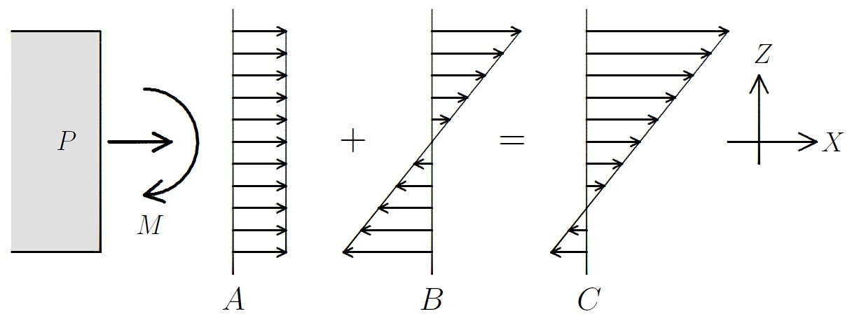
Figure 2: Superposition of stress in a beam subject to combined axial load $P$ and bending moment $M$. The cross-sectional area is $A$, on which the stress distribution due to $P$ alone is shown in (A), that due to $M$ is shown in (B), and the superposition of the two is shown in (C).

This choice is easy to justify using standard elastic theory. In the two-dimensional case, we use the superposition principle for combined loadings. For a beam with its axis lying along the $X$-axis, and with a cross-section perpendicular to this, the normal stress caused by axial loading in the direction of the positive $X$-axis (tension) is given by

$$\sigma_{x,t}=\frac{P}{A},$$ (39)

where $P$ is the force and $A$ is the cross-sectional area, see Fig. 2A. Normal stresses also arise in bending. Assuming the beam is bent within the $XZ$-plane (upper surface tensile) these stresses are

$$\sigma_{x,b}=-\frac{Mz}{I}$$ (40)

where the bending moment is $M$ and $I$ is the moment of inertia of the cross-sectional area about the neutral axis. Normal stresses are seen to depend linearly upon the vertical distance $z$ from the neutral axis, see Fig. 2B. Adding Eqs. (39) and (40) we get

$$\sigma_{x}=\sigma_{x,t}+\sigma_{x,b}$$ (41)

for the normal stress of the combined loading, that is,

$$\sigma_{x}=\frac{P}{A}-\frac{Mz}{I},$$ (42)

and the maximum $|\sigma_{x}|$ occurs along the top surface of the beam, as can be seen from Fig. 2C. In contrast, below the neutral axis (negative $z$) the normal stress due to the axial load is reduced since Eq. (40) becomes negative here. It is at its lowest along the bottom surface. If we reverse the sign on $P$ and consider compressive axial forces, we find $|\sigma_{x}|$ to be largest along the bottom surface for a beam bent like this.

A positive moment is defined as one where the beam is concave up, i.e., with the bottom surface in tension. Hence, with $z=-c$ representing the outermost fibre on the cross section,

$$\sigma=\frac{F}{A}+\frac{Mc}{I},$$ (43)

is the combined stress of axial tension and bending at this particular location. Dividing through Eq. (43) by the maximum value of the normal stress within the elastic range, $\sigma_{\rm p}$, we obtain

$$\frac{\sigma}{\sigma_{\rm p}}=\frac{F}{F_{\rm y}}+\frac{M}{M_{\rm y}},$$ (44)

where

$$F_{\rm y}=\sigma_{\rm p}A$$ (45)

is the axial force at its elastic limit, and

$$M_{\rm y}=\frac{I}{c}\hskip 1.42262pt\sigma_{\rm p}$$ (46)

is the bending moment at its elastic limit. Modeling a material which cannot deform plastically, i.e., which fails beyond the elastic limit, we can then identify $F_{\rm y}$ and $M_{\rm y}$ as breaking thresholds in $F$ and $M$. If these thresholds are denoted $t_{F}$ and $t_{M}$, one has to remove from the calculations those elements for which

$$\sigma>\sigma_{\rm p},$$ (47)

and therefore, according to Eq. (44), we must remove those elements for which the combination of $F$ and $M$ are such that

$$\frac{F}{t_{F}}+\frac{M}{t_{M}}>1$$ (48)

In our calculations we will not be interested in the details of where a ’beam’ is most stressed. What we require is to identify the maximum stress that occurs in a combined loading. In the case of axial tension Eq. (35) selects those beams where the most stressed material fibre is beyond the breaking threshold (this will be on the convex side of the beam, be that on the upper or lower surface). In the case of compression, a beam in the same bent configuration would be most stressed on the opposite surface (the concave side), and this maximum stress is still given by Eq. (35). We therefore need not distinguish between the convex and the concave sides in our application. In the discrete element model each element is either kept or removed depending on the magnitude of its greatest combined stress. The sign on $F$ or $M$ then becomes irrelevant.

For our purposes, then, elements that fail can be identified in three dimensions using

$$\frac{|F|}{t_{F}}+\frac{|M|}{t_{M}}>1,$$ (49)

where the biaxial moment is given by

$$M=\sqrt{M_{x}^{2}+M_{y}^{2}}$$ (50)

and the same thresholds $t_{\rm M}$ apply in all planes of bending.

Combined Torsion and Shear

We next consider torsion combined with transverse shear. For generality and simplicity of illustration we regard circular cross-sections. As with bending and axial force, we use the superposition principle to obtain the stress distribution for the two loads combined. From the relationship between stress and strain, generalized Hooke’s law, we have

$$\gamma=\frac{1}{G}\tau$$ (51)

We further assume for the stress distribution that

$$\tau=\frac{\rho}{R}\tau_{\rm max}$$ (52)

and for the shear strains that

$$\gamma=\frac{\rho}{R}\gamma_{\rm max},$$ (53)

where $R$ is the maximum radius of the circular cross section and

$$0<\rho<R$$ (54)

is the radial distance from the center of the cross section. Hence stress and strain increase linearly towards the outer surface where the maximum value is attained for both. The relationship between applied torque $T$ and shear stress on the cross section is

$$\tau=\frac{T}{J}\rho$$ (55)

where $J$ is the polar moment of inertia. We see from Eq. (55) that the relationship between $T$ and $\tau$ is analoguos to the relationship between $M$ and $\sigma$ in Eq. (40). For the average shear due to a vertical force we have

$$\tau=\frac{V}{A},$$ (56)

see Fig. 3B. Combining Eqs. (55) and (56),

$$\tau=\frac{V}{A}+\frac{T\rho}{J}$$ (57)

is the total shear force acting on the cross section. In Fig. 3C the two quantities are seen to oppose each other on the extreme left, while they add up on the extreme right. Torque is taken to be positive as shown, i.e., when it is a vector in the positive $X$-direction.

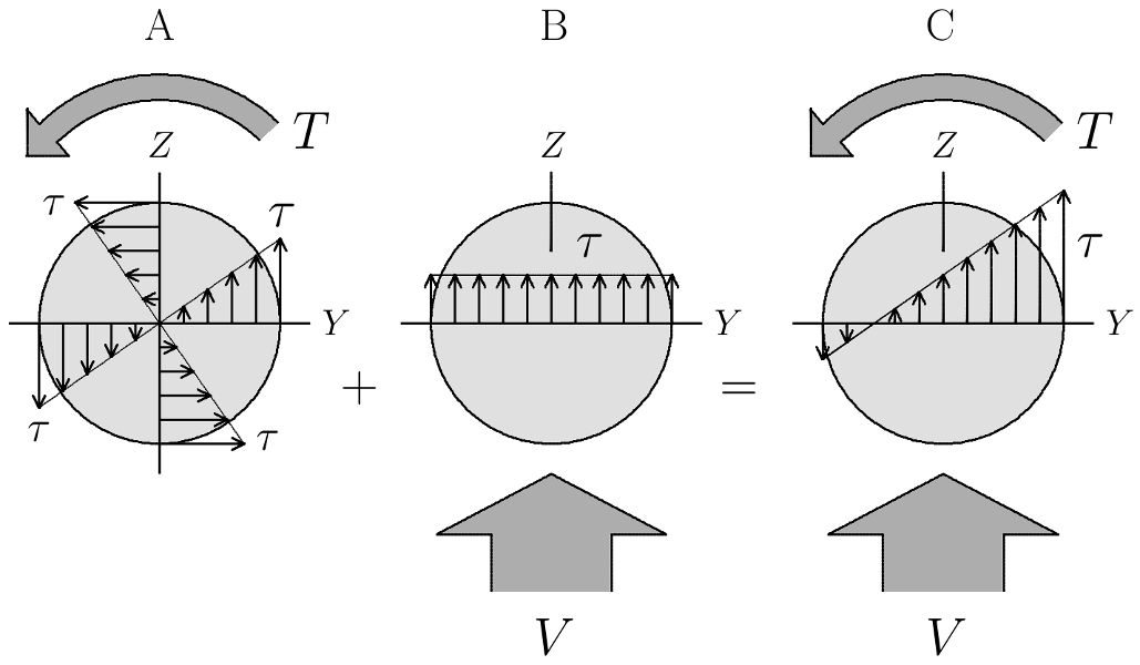
Figure 3: Distribution of shear stress on the cross section of a beam subjected to a transverse load $V$ in the direction of the positive $Z$-axis and an anti-clockwise torque $T$ about the $X$-axis. In (A) the radial distribution of stress due exclusively to torque is shown along the $Y$- and $Z$-axes, in (B) the uniform stress due to the vertical force $V$ is shown along the $Y$-axis, and in (C) the superposition of those stresses on the $Y$-axis is shown.

As before, we are not concerned with where on any particular ’beam’ the stress is highest. Instead we simply identify the maximum stress that occurs with the aim to decide whether this is above or below the breaking threshold. If the element exceeds this threshold then it is removed as a carrier of force in the elastic equations. We see that Eq. (57) is analogous to Eq. (44) for combined bending and axial force. We therefore proceed by dividing through Eq. (57) by the maximum allowable shear stress $\tau_{\rm y}$ within the elastic range. We then obtain

$$\frac{\tau}{\tau_{\rm y}}=\frac{V}{V_{\rm y}}+\frac{T}{T_{\rm y}},$$ (58)

where

$$V_{\rm y}=\tau_{\rm y}A$$ (59)

is the maximum of the transverse force $V$ in pure loading without a torque, and, from Eq. (55),

$$T_{\rm y}=\frac{J}{\rho}\tau_{\rm y}$$ (60)

is the maximum torque the element can sustain in pure rotational displacements. Assuming the element fails when

$$\tau>\tau_{\rm y}$$ (61)

our criterion for failure under combined torque and shear becomes

$$\frac{V}{t_{V}}+\frac{T}{t_{T}}>1$$ (62)

Here we have defined $t_{V}=V_{\rm y}$ and $t_{T}=T_{\rm y}$ as breaking thresholds. Requiring only the maximum stress,

$$\frac{|V|}{t_{V}}+\frac{|T|}{t_{T}}>1$$ (63)

is our fracture criterion.

As for the breaking thresholds we use one threshold for each element in our calculations. Otherwise one might be led to make inferences about the detailed structure of each ’beam’, i.e., such as where flaws are located. For instance, stress due to applied torque $T$ is at its greatest furthest away from the axis of the element, see Eq. (52), while shear stress due to a top-to-bottom vertical force $V$, according to Jourawski’s formula, is at its greatest across the centre of the section, midway between the top and bottom surfaces carp . Hence, whereas a flaw at the top or bottom surface will reduce the torque strength substantially, it will not to any great extent adversely affect the strength with which the element opposes vertical force. If one chooses to specify different thresholds for the two terms there are two obvious options. One is to assume a ’realistic’ distribution of thresholds whereby $t_{V}$ and $t_{T}$ are correlated so as to take into account different categories of flaws, the other is to simply assume that the thresholds are independently random for both types of loading. In our calculations we presently use the same threshold for both terms. This is based on the notion that ’beam’ elements are the basic building blocks in our system, i.e., they define the smallest length-scale. All heterogeneity pertaining to material flaws and/or variations in elastic properties are assumed to occur on scales at or above that of the individual discrete element.

Combined Axial Force and Shear

To obtain a general expression for the combined effects of axial force and shear we regard a body element under biaxial stress, such as that shown in Fig. 4. This body element is in a uniform state of stress. Stress being a second-order tensor, however, stress vectors vary according to the surface on which they act. In the following we regard a plane which intersects the body element at a given angle and observe how the components vary as the angle is varied chou , see Fig. 5. Here the $X^{\prime}Y^{\prime}$-coordinate system has been rotated through an angle $\alpha$, such that the $X^{\prime}$-axis coincides with the normal to the inclined plane. For a body element in equilibrium, the stress vector $\bm{p}$ acting on this plane is obtained by requiring the sum of forces to be zero. If we resolve the vector $\bm{p}$ in the $XY$-coordinate system, we obtain

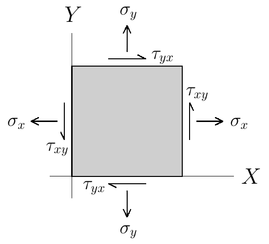
Figure 4: Elastic body element showing components of normal stress, $\sigma_{x}$ and $\sigma_{y}$, and components of shear, $\tau_{xy}$ and $\tau_{yx}$, on those surfaces that are parallel to the $Z$-axis.

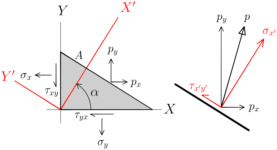
Figure 5: Free body with stress components on all surfaces. Decomposition of the stress vector $\bm{p}$ relative to the $X^{\prime}Y^{\prime}$-coordinate system is shown in red, decomposition relative to the $XY$-coordinate system is shown in black. The surface area of the inclined plane is $A$.

$$\bm{p}=\bm{p}_{x}+\bm{p}_{y},$$ (64)

the components of which are found to be

$$p_{x}=\sigma_{x}\cos\alpha+\tau_{xy}\sin\alpha$$ (65)

and

$$p_{y}=\sigma_{y}\sin\alpha+\tau_{xy}\cos\alpha$$ (66)

However, $\bm{p}$ can also be resolved in the $X^{\prime}Y^{\prime}$-coordinate system. Expressing first $\sigma_{x^{\prime}}$ and $\tau_{x^{\prime}y^{\prime}}$ in terms of $p_{x}$ and $p_{y}$, as shown on the right in Fig. 5, Eqs. (65) and (66) are next used to obtain $\sigma_{x^{\prime}}$, $\sigma_{y^{\prime}}$ and $\tau_{x^{\prime}y^{\prime}}$ in terms of $\sigma_{x}$, $\sigma_{y}$ and $\tau_{xy}$. We thus obtain

$$\sigma_{x^{\prime}}=\frac{\sigma_{x}+\sigma_{y}}{2}+\frac{\sigma_{x}-\sigma_{y}}{2}\cos 2\alpha+\tau_{xy}\sin 2\alpha$$ (67)

and

$$\sigma_{y^{\prime}}=\frac{\sigma_{x}+\sigma_{y}}{2}-\frac{\sigma_{x}-\sigma_{y}}{2}\cos 2\alpha-\tau_{xy}\sin 2\alpha$$ (68)

for the normal stresses, and

$$\tau_{x^{\prime}y^{\prime}}=\frac{\sigma_{y}-\sigma_{x}}{2}\sin 2\alpha+\tau_{xy}\cos 2\alpha$$ (69)

for the shear stress in the $X^{\prime}Y^{\prime}$-system. These are known as the transformation of stress equations chou , and allow us to determine the stress on any plane when the angle $\alpha$ and the stresses $\sigma_{x}$, $\sigma_{y}$ and $\tau_{xy}$ are known.

We next seek the extreme values of stress by varying the orientation of the inclined plane. Assuming structural integrity to be exceeded when the normal stress reaches a critical value, we evaluate

$$\frac{{\rm d}\sigma_{x^{\prime}}}{{\rm d}\alpha}=0$$ (70)

to obtain

$$\tan 2\alpha=\frac{2\tau_{xy}}{\sigma_{x}-\sigma_{y}}$$ (71)

This expression implies two solutions for $\alpha$ which are $90^{\circ}$ apart. We also see that Eq. (71) is identical to Eq. (69), provided that $\tau_{x^{\prime}y^{\prime}}=0$. Extreme values of normal stress are therefore obtained where shear stress vanishes.

Substituting the angles which satisfy Eq. (71) into Eq. (67) we obtain, after a few manipulations,

$$\sigma_{x^{\prime}}=\frac{\sigma_{x}+\sigma_{y}}{2}+\sqrt{\bigl{(}\frac{\sigma_{x}-\sigma_{y}}{2}\bigr{)}^{2}+\tau_{xy}^{2}}$$ (72)

for the maximum normal stress. ’Beam’ elements in our model are force carriers between lattice nodes, hence there is no normal stress perpendicular to the connecting line between these and Eq. (72) becomes

$$\sigma_{\rm m}=\frac{\sigma_{x}}{2}+\sqrt{\bigl{(}\frac{\sigma_{x}}{2}\bigr{)}^{2}+\tau_{xy}^{2}},$$ (73)

where the maximum value of $\sigma_{x^{\prime}}$ has been denoted $\sigma_{\rm m}$. This expression is divided through by the failure threshold $\sigma_{\rm f}$ for the normal stress obtained in pure axial loading, to give

$$\frac{\sigma_{\rm m}}{\sigma_{\rm f}}=\frac{R_{\sigma}}{2}+\sqrt{\bigl{(}\frac{R_{\sigma}}{2}\bigr{)}^{2}+\bigl{(}kR_{\tau}\bigr{)}^{2}},$$ (74)

where we have introduced the dimensionless ratios of normal and shear stress to their respective failure thresholds,

$$R_{\sigma}=\frac{\sigma_{x}}{\sigma_{\rm f}},\qquad R_{\tau}=\frac{\tau_{xy}}{\tau_{\rm f}},$$ (75)

as well as the parameter

$$k=\frac{\tau_{\rm f}}{\sigma_{\rm f}}$$ (76)

for the ratio of the shear and normal failure stresses. This ratio, for steel, is often taken to be in the range $0.5-0.75$. For rocks the ratio of tensile to shear strength corresponds to roughly $k\sim 1$, while the compressive strength is at least ten times higher than the tensile strength afro . Assuming that our material fails when

$$\sigma_{\rm m}>\sigma_{\rm f},$$ (77)

our criterion for when a ’beam’ element fails is

$$\frac{F}{2t_{F}}+\sqrt{\bigl{(}\frac{F}{2t_{F}}\bigr{)}^{2}+\bigl{(}k\frac{V}{t_{V}}\bigr{)}^{2}}>1,$$ (78)

where in Eq. (74) loads and failure loads have been substituted for stresses and failure stresses.

Assuming instead that material integrity is exceeded when shear stress reaches a critical value,

$$\frac{{\rm d}\tau_{x^{\prime}y^{\prime}}}{{\rm d}\alpha}=0$$ (79)

is evaluated to obtain

$$\tan 2\alpha=-\frac{\sigma_{x}-\sigma_{y}}{2\tau_{xy}},$$ (80)

the right-hand side of which is the negative reciprocal of Eq. (71). This implies that the planes of maximum shear are at an angle of $45^{\circ}$ with respect to the planes of maximum normal stress chou .

From Eq. (80) expressions for $\cos{2\alpha}$ and $\sin{2\alpha}$ are obtained which are substituted into Eq. (69). This gives

$$\tau_{x^{\prime}y^{\prime}}=\sqrt{\bigl{(}\frac{\sigma_{x}-\sigma_{y}}{2}\bigr{)}^{2}+\tau_{xy}^{2}}$$ (81)

for the maximum shear stress. As with Eq. (72) there is no normal stress perpendicular to the connecting line between nodes and

$$\tau_{\rm m}=\sqrt{\bigl{(}\frac{\sigma_{x}}{2}\bigr{)}^{2}+\tau_{xy}^{2}}$$ (82)

is obtained by setting $\sigma_{y}=0$. Assuming the material fails for

$$\tau_{\rm m}>\tau_{\rm f},$$ (83)

where $\tau_{\rm f}$ is the failure threshold for the shear stress, and dividing through Eq. (82) by this quantity, we get

$$\tau_{\rm m}=\sqrt{\bigl{(}\frac{R_{\sigma}}{2k}\bigr{)}^{2}+R_{\tau}^{2}}$$ (84)

using the first of Eqs. (75), and Eq. (76). The criterion for when a ’beam’ element should break is then

$$\sqrt{\bigl{(}\frac{F}{2kt_{F}}\bigr{)}^{2}+\bigl{(}\frac{V}{t_{V}}\bigr{)}^{2}}>1,$$ (85)

where in Eq. (84) we have substituted loads and failure loads for stresses and failure stresses.

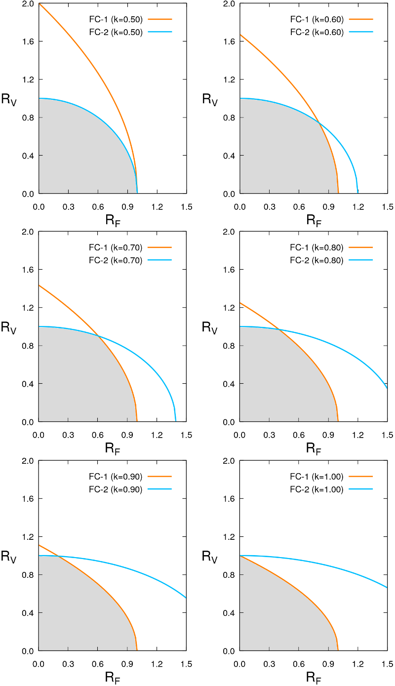
Figure 6: Failure envelopes corresponding of Eqs. (78) and (85), presently denoted FC-1 and FC-2, shown for $k=0.5$, $k=0.6$, $k=0.7$, $k=0.8$, $k=0.9$ and $k=1.0$. The expressions $R_{F}$ and $R_{V}$ are the dimensionless ratios $F/t_{F}$ and $V/t_{V}$, respectively, of the load to failure loads.

Plotting Eqs. (78) and (85) for different values of $k$ it is seen that Eq. (78) with $k=1$ and Eq. (85) with $k=0.5$ provide interaction curves where the expressions

$$\frac{F}{t_{F}}<1,\qquad\frac{V}{t_{V}}<1$$ (86)

are both satisfied, see Fig. 6. For values of $k$ between $0.5$ and $1$ the failure envelope is a combination of Eqs. (78) and (85), corresponding to the innermost region bounded by the yellow and blue curves in Fig. 6 (these have been shaded in gray). Eq. (85) with $k=0.5$, according to Refs. nasa and rjwi , provides a convenient and conservative interaction curve when considering combined shear and axial loading, this is the shaded region enclosed entirely by the blue curve in the upper left pane of Fig. 6. Hence, we choose

$$\sqrt{\bigl{(}\frac{F}{t_{F}}\bigr{)}^{2}+\bigl{(}\frac{V}{t_{V}}\bigr{)}^{2}}>1$$ (87)

as our criterion. For $k\rightarrow 0.5$ we see from Fig. 6 that the shaded region approaches this criterion, while it approaches

$$\frac{F}{2t_{F}}+\sqrt{\bigl{(}\frac{F}{2t_{F}}\bigr{)}^{2}+\bigl{(}\frac{V}{t_{V}}\bigr{)}^{2}}>1$$ (88)

when $k\rightarrow 1$ (the yellow curve in the bottom right window). From Fig. 6 it is also evident that Eq. (87) is a good fit within the greater part of the range $0.5<k<1$, deviating the most for values above $k\simeq 0.9$. For comparison, we will nonetheless also include results obtained with Eq. (88) to see if this slightly more conservative alternative makes any difference.

Combined Axial Force, Shear, Torsion and Bending

Finally we seek an interaction formula which combines axial force, shear, bending and torsion. The basic form of the fracture criterion is taken to be the interaction between axial force and shear, as given by Eq. (87) or Eq. (88). Within this prescription, bending is considered in combination with axial force, and torsion is considered as a contribution to shear.

With Eq. (87) as our basic expression, the fracture criterion is then

$$\sqrt{\bigl{(}\frac{\widehat{F}}{t}\bigr{)}^{2}+\bigl{(}\frac{\widehat{V}}{t}\bigr{)}^{2}}>1$$ (89)

where

$$\widehat{F}=|F|+|M|$$ (90)

is the total stress due to deformations which cause elongation, as shown in Fig. 2, and

$$\widehat{V}=|V|+|T|$$ (91)

is the total stress from deformations contributing to shear, as shown in Fig. 3. Note that in Eq. (89) we have also assumed the same breaking threshold for loading in shear and tension, that is

$$t=t_{F}=t_{V}$$ (92)

In three dimensions the shear force $V$ in Eq. (91) acts within two perpendicular planes. If we consider beam $1$ in Fig. 1, extending along the positive $X$-axis, shear within the $XZ$- and $XY$-planes are combined into a bi-planar expression in Eq. (91). Hence, we have

$$|V|=\sqrt{V_{XY}^{2}+V_{XZ}^{2}},$$ (93)

where $V_{XY}$ and $V_{XZ}$ are the respective contributions acting within the two planes. Likewise, in Eq. (90) axial force $F$ is combined with the largest of the moments at the ends of the ’beam’ element, i.e.,

$$|M|={\rm max}\bigl{(}M_{i},M_{j}\bigr{)}$$ (94)

where $i$ is the near (node) end and $j$ is the far (neighbouring node) end of the ’beam’ element. If we again consider beam 1 we now have

$$M_{i}=\sqrt{M_{y,i}^{2}+M_{z,i}^{2}},$$ (95)

with $M_{y,i}$ and $M_{z,i}$ representing the contributions from bending obtained within the $XZ$- and $XY$-planes, respectively ($M_{y}$ is the bending moment about the cross-sectional centroidal axis $Y$). The expression for $M_{j}$ is similar.

Finally, for the sake of comparison, the $k=1$ criterion based on maximum normal stress is also included. Hence, Eq. (88) reads

$$\frac{\widehat{F}}{2t}+\sqrt{\bigl{(}\frac{\widehat{F}}{2t}\bigr{)}^{2}+\bigl{(}\frac{\widehat{V}}{t}\bigr{)}^{2}}>1,$$ (96)

where the quantities $\widehat{F}$, $\widehat{V}$ and $t$ are given by the same expressions as those in Eq. (89) above.

Although a ’beam’ element, when regarded as a separate entity, can be strained, twisted and deformed in all manner of ways, we regard independent couplings between torsion and bending as less significant. Interaction between these two effects is still included, but only indirectly in the sense that bending contributes to axial stress, and torsion to shear, before the two are combined via Eqs.(87) or (88). This also applies to the combination of shear and bending, and to the combination of axial deformation and torsion – any direct interaction between these effects is assumed negligible.

Our assumption of a fracture criterion taking this form is not unreasonable considering the fact that we intend to model a continuum, within which the ’beam’ is embedded and thereby considerably constrained by the surrounding medium. The situation would be different in considering an isolated beam which can move freely, and even more so if this beam is of the slender type or has a cross-sectional geometry that is important in the overall context. Moreover, in modeling a discretized continuum, realistic forces between nodes should preclude the use of discrete elements based on slender beams.

V Illustration of Stresses in Combined Loads

In order to substantiate how stresses are distributed throughout a structure when combined loadings are applied we can construct ’macroscopic’ beams from discrete elements. Based on a cubic lattice morphology, the simplest such structure is a square prism. Structures with other cross-sections are obtained by

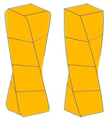
Figure 7: A square prism beam deformed in torsion. The top surface has been rotated $45^{\circ}$ clockwise and the bottom surface $45^{\circ}$ counter-clockwise. Version based on linear equations is shown on the left, and version based on non-linear equations is shown on the right.

cutting away beams that lie outside the required geometric profile. Circular or elliptic cross-sections, for instance, are easily obtained in this way. Presently we regard beams with square cross-sections and marked outlines, since it is easier to visualize deformations (especially torsion) this way.

Deformations are best visualized when they are sizeable. The displacements involved in our calculations for the roughness exponent, on the other hand, are quite small. This is appropriate in a brittle fracture study, since the external displacements involved are usually small. Large deformations are more commonly associated with ductile materials. However, in order to illustrate a few cases of how stresses are altered as different modes of external loading are combined, we employ large displacements for visual effect. If we use Eqs. (27) to (32) for this purpose a ’warping’ effect is obtained when angular displacements become large. This is shown on the left in Fig. 7, where the top and bottom surfaces have been rotated in opposite directions. Edges near the top and bottom are seen to turn inwards after a gradual swelling develops as the ends are approached. The reason why the effect is most marked near the ends is because it is here that rotational displacements are largest.

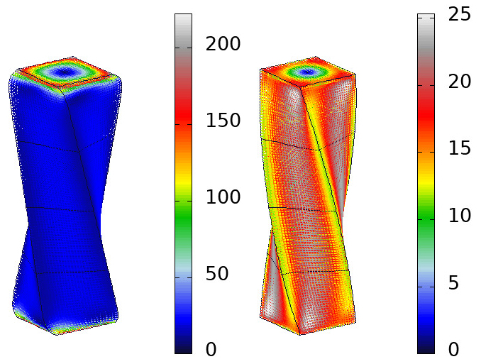
Figure 8: Shear stresses in square beam with large torsionl deformations. Version based on linear equations is shown on the left, and version based on non-linear equations is shown on the right.

In contrast to this is the version shown on the right in Fig. 7. Here, the axial contributions from the beams have been corrected to take into account the rotations about three axes. Components of shear and bending moment should also be adjusted in this way, leading to equations which involve a large number of terms. However, provided deformations are not too extreme, corrections applied to the axial terms are the most important. In Fig. 7 the rotation of the top and bottom surfaces is 45 degrees, for a total rotation of 90 degrees between top and bottom. For such a large deformation the version on the right represents a dramatic improvement over the one on the left. The relevant modifications to Eqs. (27), (28) and (29) are

$$X_{i}= -\frac{1}{\alpha}\sum_{j=1}^{6}\widehat{\lambda}_{1,3}\bigl{(}1-\sqrt{A_{j}}\hskip 1.42262pt\bigr{)}s_{j}\Phi_{j}-\frac{1}{\beta+\frac{\gamma}{12}}\sum_{j=1}^{6}\widehat{\chi}_{1,3}\biggl{\{}\delta x_{j}+\frac{r_{j}}{2}\Bigl{[}\widehat{\lambda}_{5,6}\bigl{(}v_{i}+v_{j}\bigr{)}+\widehat{\lambda}_{2,4}\bigl{(}w_{i}+w_{j}\bigr{)}\Bigr{]}\biggr{\}},$$ (97)

for the $X$-component of force on node $i$,

$$Y_{i}= -\frac{1}{\alpha}\sum_{j=1}^{6}\widehat{\lambda}_{2,4}\bigl{(}1-\sqrt{A_{j}}\hskip 1.42262pt\bigr{)}s_{j}\Phi_{j}-\frac{1}{\beta+\frac{\gamma}{12}}\sum_{j=1}^{6}\widehat{\chi}_{2,4}\biggl{\{}\delta y_{j}+\frac{r_{j}}{2}\Bigl{[}\widehat{\lambda}_{5,6}\bigl{(}u_{i}+u_{j}\bigr{)}+\widehat{\lambda}_{1,3}\bigl{(}w_{i}+w_{j}\bigr{)}\Bigr{]}\biggr{\}}$$ (98)

for the $Y$-component, and

$$Z_{i}= -\frac{1}{\alpha}\sum_{j=1}^{6}\widehat{\lambda}_{5,6}\bigl{(}1-\sqrt{A_{j}}\hskip 1.42262pt\bigr{)}r_{j}\Phi_{j}-\frac{1}{\beta+\frac{\gamma}{12}}\sum_{j=1}^{6}\widehat{\chi}_{5,6}\biggl{\{}\delta z_{j}-\frac{s_{j}}{2}\Bigl{[}\widehat{\lambda}_{2,4}\bigl{(}u_{i}+u_{j}\bigr{)}+\widehat{\lambda}_{1,3}\bigl{(}v_{i}+v_{j}\bigr{)}\Bigr{]}\biggr{\}},$$ (99)

for the $Z$-component. Here

$$A_{j} = \widehat{\chi}_{1,3}\hskip 1.42262pt\delta x_{j}^{2}+\widehat{\lambda}_{1,3}\bigl{(}1-r_{j}\delta x_{j}\bigr{)}^{2}+\widehat{\chi}_{2,4}\hskip 1.42262pt\delta y_{j}^{2}+\widehat{\lambda}_{2,4}\bigl{(}1+r_{j}\delta y_{j}\bigr{)}^{2}+\widehat{\chi}_{5,6}\hskip 1.42262pt\delta z_{j}^{2}+\widehat{\lambda}_{5,6}\bigl{(}1+r_{j}\delta z_{j}\bigr{)}^{2}$$

is the squared length of the discrete element between nodes $i$ and $j$ (disregarding curvature). Furthermore,

$$\Phi_{j}=\widehat{\lambda}_{1,3}\cos{v_{i}}\cos{w_{i}}+\widehat{\lambda}_{2,4}\cos{u_{i}}\cos{w_{i}}+\widehat{\lambda}_{5,6}\cos{u_{i}}\cos{v_{i}}$$ (100)

is the angular displacement of node $i$. As can be seen from Fig. 7, the version on the right is clearly free of the warping seen in the version on the left.

The importance of taking into account local rotations for large deformations is made even more clear if we regard the stresses involved. In Fig. 8 the shear stresses involved in the two cases are shown, and the colour scales included with the beams illustrate the point. Evidently, when using linear equations, the stresses involved near the ends of the beam become quite extreme, almost ten times higher than elsewhere in the beam. Away from the ends, however, the stresses are comparable, as can be seen from the colour scales. In contrast, a uniform distribution of shear is obtained with Eqs. (97) to (99) in place of Eqs. (27) to (29).

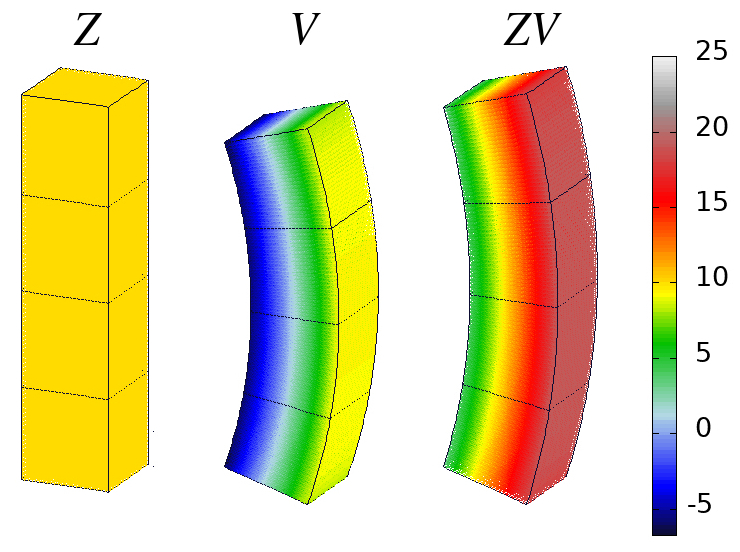
Figure 9: A square prism beam structure, sides $L=25$ and height $H=101$, loaded in tension (Z), pure bending (V), and the two combined (ZV).

The relevant equations are more complicated, and involve non-linear terms which necessitate an iterative adaption of conjugate gradients. In this approach the decreasing residuals of each successive solution are adopted as a starting point for a new tentative solution. Hence, at each stage in the breaking process a loop produces a sequence of tentative solutions. Within this loop, the number of iterations required for each successive solution decreases rapidly until the solution has converged. Although computational time increases significantly in comparison with the linear set of equations, it is still a only a matter of a minute or two to obtain stress distributions for relatively large structures. Such structures may be intact or at a pre-determined stage of breaking. However, for the purpose of studying the entire fracture process it is more practical to use linear equations in conjunction with small deformations.

We consider a beam in the form of a square prism, where all edges have been drawn black as an aid to emphasize body shape and displacements. External loads are imposed by rotating or translating the top and bottom surfaces of the body. The combination of bending and axial tension discussed in Section IV is illustrated in Fig. 9 in the case of a beam with length $4L$. Additional black lines in the figure delineate cubes with sides $L=25$. On the left is a beam that is loaded in the vertical direction (stretched along the $Z$-axis), in the middle is the same beam in a bent configuration only (bending within the $XZ$-plane), and on the right the two loadings are combined. Stresses shown are axial stresses in discrete elements aligned along the vertical axis (the $Z$-axis). Referring to the colour scale (the same scale relates to all three loadings) axial stresses of the tensile and bending cases are clearly seen to be additive, as expected from the superposition of forces in Eq. (49).

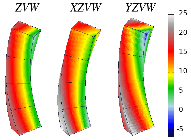
Figure 10: A square prism beam, with sides $L=25$ and height $H=101$, loaded in tension and bending (ZV), with added torsion (ZVW) and shear (XZVW and YZVW).

Table 1: Average forces summed from top to bottom along the middle of the vertical sides of a structure with square cross-section, sides $L=25$ and height $H=101$, with the structure having been subjected to different external loadings. Loading types denoted $X$, $Y$ and $Z$ represent translations of the upper surface along said positive axes. Size of the translations in all cases corresponds to 10 discrete element lengths. Loadings denoted $U$, $V$ and $W$ are rotations about axes parallel with the $X$-, $Y$-, and $Z$-axes, respectively. In all such cases the bottom surface has been rotated $+0.1\pi$ while the top surface has been rotated $-0.1\pi$. The side facing the viewer is denoted ’000’, other sides being ’090’ (right), ’180’ (opposite) and ’270’ (left).

	Axial average					Shear average
	Loading	$\sum_{Z}F_{090}$	$\sum_{Z}F_{270}$			Loading	$\sum_{Z}V_{000}$	$\sum_{Z}V_{180}$
	Z	10.00	10.00			X	5.07	5.07
	V	9.15	-5.93			W	9.67	9.67
	Eq. (90)	19.15	4.07			Eq. (91)	4.60	14.74
	ZV	19.00	3.93			XW	4.76	14.57
	ZVW	19.49	4.03			XWV	6.42	12.96
	YZVW	20.52	3.78			XZWU	6.25	13.14
	XZVW	19.92	4.46			XWUV	4.77	14.60

In the figure, positive values are tensile while negative values are compressive. Average axial forces, obtained by summing from top to bottom along the middle of the vertical faces of the beam are included in Table 1. Here, $\sum F_{090}$ and $\sum F_{270}$ refer to the convex and concave sides of the beam, respectively, in Fig. 9 The reason we consider average values of axial force is because we presently regard the $25\times 25\times 101$ square prism as a model of a discrete element ’beam’. In a fracture criterion we will not be interested in details pertaining to scales smaller than that of each element.

Table 1 shows that values obtained by adding ’$Z$’ and ’$V$’, as dictated by Eq. (90), agree well with the actual values obtained in the combined loading, denoted ’$ZV$’ in Fig. 9. To what extent will additional loadings alter this picture? Instead of carrying out a systematic investigation involving many data points, a few extra loads added onto the ’ZV’ combinations have been included in the last three lines of Table 1. These are torsion, ’ZVW’, as well as torsion and shear, ’YZVW’ and ’XZVW’. In the latter cases the top surface has been translated along the positive $Y$- and $X$-axes, respectively. Although the displacements and rotations involving all the loadings are quite sizeable the average axial forces on the convex ($\sum F_{090}$) and concave ($\sum F_{270}$) sides do not change much, relatively speaking, as can be seen from the values in Table 1. Hence, the task of identifying the largest contribution from axial forces seems to be adequately taken care of by the first term, $\widehat{F}/t$, in Eq. (89). Had we considered the detailed distribution of forces rather than the averages, the highest axial force in the ’YZVW’ and ’XZVW’ cases would have been found to occur in discrete elements that are situated in the corners of the cross-section, near the top and bottom surfaces, on the concave side of the structure (see the colour scale in Fig. 10). Numerical values in these two cases are about 20% higher than the averages quoted in Table 1. Maximum axial stress in the ’ZVW’ case is only about 5% higher and occurs in a corner about three quarters of the way towards the top surface. In this context we also have to keep in mind that these values refer to cross-sections that are square rather than circular.

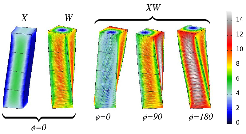
Figure 11: Beam of square cross-section, sides $L=25$ and height $H=101$, made up of discrete elements. The structure has been subjected to shear (X), torsion (W) and both these loadings combined (XW). Here, $\phi\neq 0$ is a counter-clockwise rotation of the structure. Hence $\phi=90$ has turned the side corresponding to $\sum_{Z}V_{090}$ towards the viewer.

Table 1 also includes average shear forces calculated along the vertical faces of the square prism structure. Hence, the combination of shear and torsion, and to what extent this is affected by other loading modes, is investigated next. In Fig. 11 is shown a beam under pure shear, pure torsion and the combination of these two loadings. The combined loading has been shown from three different angles, illustrating how shear on one side increases while that on the other side decreases, in accordance with the superposition of forces in Eq. (91).

On the extreme left is a beam where the top surface has been translated along the positive $X$-axis. The shear force is seen to be at its largest in the middle of the cross-section and decreases to zero at the edges. This is an example of Jourawski’s formula, i.e.,

$$\tau=\frac{V_{x}Q_{y}}{I_{y}L},$$ (101)

where

$$Q_{y}=\int_{A}x{\rm d}A$$ (102)

is the first, or static, moment of area about the axis of bending (the $Y$-axis in this case), $I_{y}$ is the moment of inertia about the same axis, and $L$ is the width of the cross-section. For a square cross-section the distribution of forces across the width is in the shape of a parabola. This is so because the external transverse force $V_{x}$ produces a bending moment which varies along the length of the structure carp , i.e., the $Z$-axis in this case. The distribution of shear forces is shown in

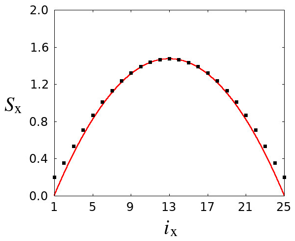
Figure 12: Shear force variation across the width of the mid-section of a $25\times 25\times 201$ square beam, with parabola shown in red.

Fig. 12 for a structure which has sides $L=25$ and vertical length (or height) $8L$. The external force $V_{x}$ arises from a horizontal translation of the top surface a distance of 15 discrete elements. Numerical values are shown as solid squares and have been obtained along a line through the centre of the cross-section, midway between the top and bottom surfaces. A parabola, shown in red, has been fit to these values. Apart from at the very edges, the numerical values are seen to conform very well to the shape predicted by Jourawski’s formula. The discrepancy at the edges are finite-size effects, as can be seen by making finer the resolution of the discretization. Increasing proportionally the dimensions of the sample and the magnitude of the external deformation, the effect obtained is analogous to such a refinement of numerical resolution. One example of this is included in Fig. 13, which shows the distribution of shear forces in a structure with sides $L=51$ and height $8L$. Here the external

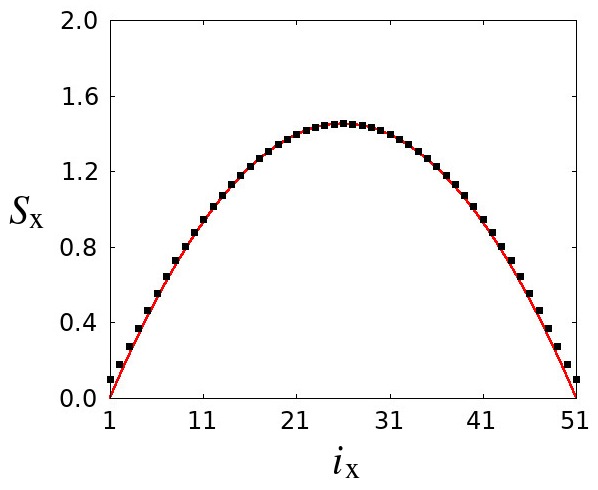
Figure 13: Shear force variation across the width of the mid-section of a $51\times 51\times 409$ square beam, with parabola shown in red.

transverse displacement used is 30 discrete elements, and the discrepancy at the edges between the numerical values and the parabola is now seen to be much smaller.

The next beam in Fig. 11, denoted ’W’, is under pure torsion, and following this is the ’XW’ case where the two loadings ’X’ and ’W’ are combined. As expected, values in Table 1 obtained for the average forces on the sides where shear increases or decreases compare favourably with values expected from Eq. (91), i.e., shear intensifies on one side and is alleviated on the other. The interesting question is to what extent other deformations influence this relationship. Adding a bending moment ’V’ or a biaxial bending moment ’UV’ changes the values somewhat (see Table 1, but not anywhere near what would be required to invalidate the relationship between ’X’ and ’W’ as incorporated into Eq. (89) by the term $\widehat{V}/t$. The distribution of forces involved when adding the biaxial moment ’UV’ are shown in Fig. 14.

Breaking Thresholds

The breaking thresholds for the two terms in Eq. (89) have been set to the same value in Eq. (92) since we wish to avoid making inferences about the detailed structure of each ’beam’. If a ’beam’ is axially weak we also assume that it will be weak in shear, bending and torsion. We will not devise

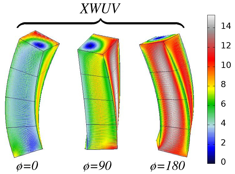
Figure 14: A square prism beam, with sides $L=25$ and height $H=101$, subject to shear (X), torsion (W) and biaxial bending (U and V).

individual threshold distributions based on where ’flaws’ in a ’beam’ might be located. Otherwise one might, for instance, expect a ’beam’ with an edge crack to be unaffected in strength when bent such that the edge crack is compressed (closed) while weakened when it is bent the other way. Likewise, a ’beam’ with a central flaw might be expected to show structural resilience towards bending in either plane while being weakend in axial strength. We may still adjust the thresholds so that the ’beam’ is proportionally weaker in tension than in shear. This can be done, for instance, by multiplication with a constant factor. The main point is that all thresholds relevant to any given ’beam’ is chosen from a single value in the stochastic distribution.

VI External Uniaxial Tension on a Cube

Using the model described in Section II, tensile fracture is initiated by imposing a uniform displacement vertically (along the $Z$-axis) on the top surface of the lattice. The edges of the cube are taken to be parallel with the coordinate axes. Discrete elements are removed one at a time, and at any stage in the fracturing process Eq. (13) is used to calculate new displacements after a discrete element has been removed. The resulting distribution of stress, in conjunction with the breaking thresholds assigned, is used to identify which discrete element will break next. Exactly how this identification is made relies on the nature of the fracture criterion.

Fracture surfaces obtained for three different samples of size $L=32$ are shown in Fig. 15. The disorder used is one of intermediate strength, corresponding to $D=1$ in the prescription outlined in Section III. For each sample the only difference between the one on the left and its counterpart on the right is the fracture criterion used. Samples on the left have been broken with the original fracture criterion, Eq.(34), while Eq.(89) has been used for those on the right. For the three samples shown the fracture surfaces appear roughly at the same position vertically on the lattice. Slopes, elevated areas and depressions sometimes also appear in the same locations. Although some samples appear superficially similar for the two fracture criteria, others again differ substantially. A closer look at the three samples in Fig. 15, however, reveals an important difference between fracture surfaces obtained with these two criteria. This difference, moreover, pertains to all samples. Specifically, those obtained

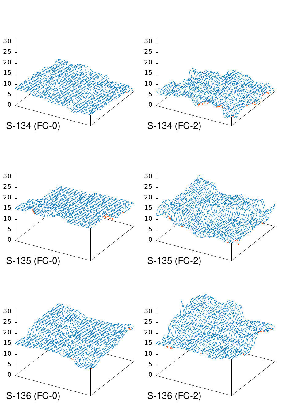
Figure 15: Comparison of fracture surfaces obtained with different fracture criteria. Three different samples are shown, S-134, S-135 and S-136. FC-0 denotes the ’original’ criterion, Eq. (34), and FC-2 denotes the ’maximum shear stress’ criterion, Eq. (89). Fracture interfaces are red on the underside and blue on top.

with Eq. (89) display a pronounced roughness, in stark contrast with those obtained with Eq. (34). In the latter case fracture surfaces are seen to consist of flat sections that are stepped up or down relative to each other – reminiscent of a landscape of ’plateaus’. Fracture surfaces evidently look very different depending on which of the two criteria one uses.

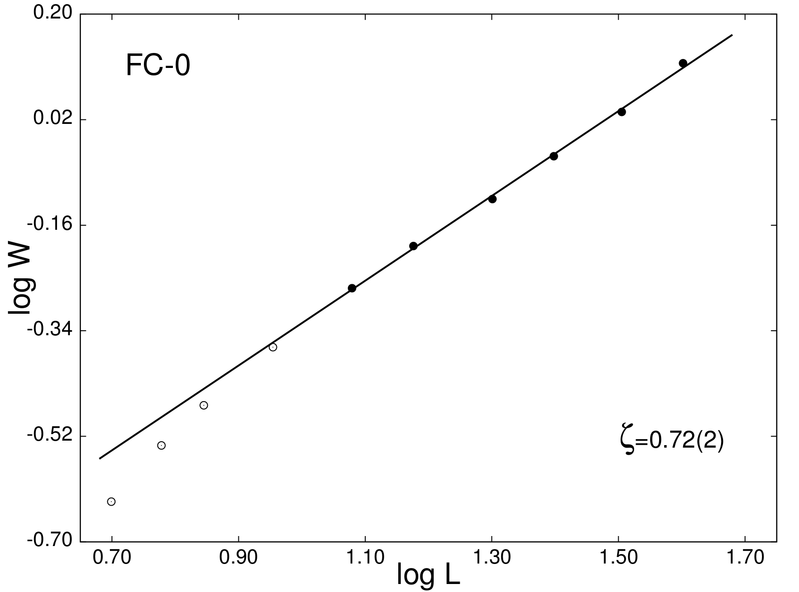
Figure 16: Log-log plot showing average roughness, $W$, as a function of system size, $L$, for a large number of fractured samples of each size. Disorder magnitude is $D=1.5$. (FC-0) denotes the result obtained with the ’original’ fracture criterion, Eq. (34).

Such a difference in appearance could, however, also be obtained with the same fracture criterion by increasing or decreasing the magnitude of structural disorder skj2 . The question is: does the morphology change in more fundamental ways than just to provide an offset in the roughness with respect to disorder strength? To answer this we turn to a standard yardstick in brittle fracture calculations, i.e., the exponent which characterizes how surface roughness scales with system size mand ; darc ; smod ; adva . Fracture surfaces have been found to be self-affine, meaning that if lengths within the fracture plane are scaled by a factor $\lambda$ then lengths perpendicular to this plane scale by a factor $\lambda^{\zeta}$, where $\zeta$ is the roughness exponent. A self-affine relationship $W\sim L^{\zeta}$ is therefore obtained, and this appears as a straight line in a log-log plot. Results in 3D have been obtained for $\zeta$ with various models, such as the random fuse model batr ; rais ; alav ; nuka , which is an electrical analogue to fracture, and with networks of elastic springs pari . Results have also been obtained with the beam lattice skj2 ; bara with results varying according to the fracture criterion used, and possibly also with other parameters involved, such as disorder.

Quantification of surface roughness is done in the same way as in Ref. skj2 , i.e., as the root-mean-square variance perpendicular to the fracture plane,

$$W_{x}(L)=\left\langle\frac{1}{L}\sum_{i=1}^{L}z_{x}(i)^{2}-\biggl{[}\frac{1}{L}\sum_{i=1}^{L}z_{x}(i)\biggr{]}^{2}\right\rangle^{1/2},$$ (103)

where $z_{x}(i)$ is the vertical height of the first intact node encountered when moving down towards the lower remaining part of the structure (shown in Fig. 15).

Previous calculations made with the ’original’ criterion, Eq. (34), indicates a roughness exponent $\zeta$ which varies considerably with the magnitude of the disorder skj2 , i.e., $0.59<\zeta<0.78$. Here the smaller values $\zeta\sim 0.6$ correspond to strong disorder, $|D|\geq 2$, and larger values $\zeta\sim 0.8$ to intermediate disorder, $D=1$. These exponents are therefore somewhat high compared with the large-scale experimental result, $\zeta\simeq 0.5$ boff ; pons . In Fig. 16 we show the roughness exponent obtained with the ’original’ criterion Eq. (34), using $D=1.5$. Not surprisingly the result, $\zeta=0.72$, lies between the results obtained for $D=1$ and $D=2$ in Ref. skj2 , that is, it lies between between $\zeta=0.78$ and $\zeta=0.62$. Using Eq. (89), however, the value of the exponent reduces to the much lower value of $\zeta=0.52$, very close to the experimentally reported value for large length scales. This is notable in light of the fact that

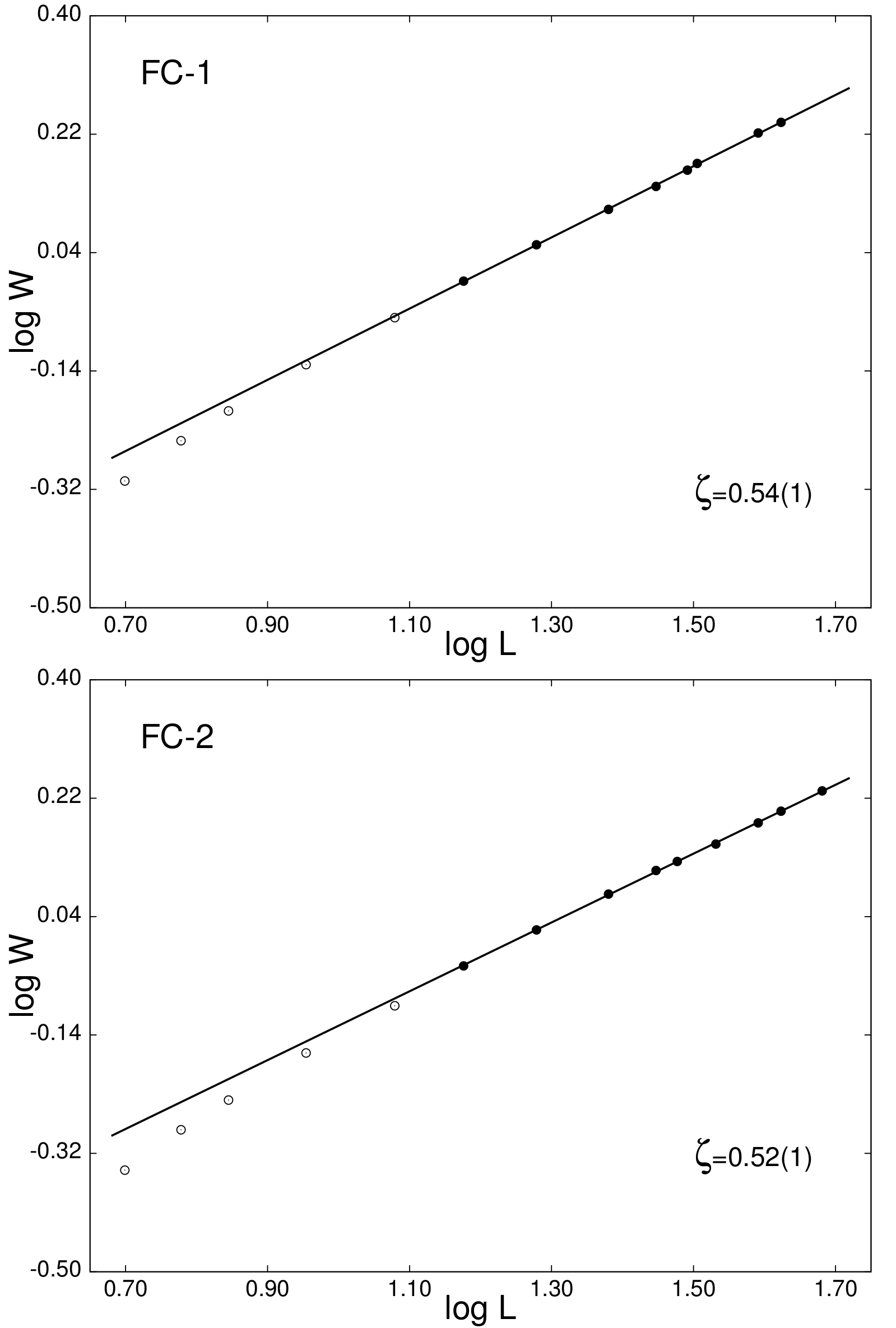
Figure 17: Log-log plots for average roughness, $W$, as a function of system size, $L$, for a large number of fractured samples. Disorder magnitude is $D=1.5$. Shown at the top (FC-1) is the result obtained with the ’maximum normal stress’ criterion, Eq. (96). Shown below (FC-2) is the result obtained with the ’maximum shear stress’ criterion, Eq. (89).

the original criterion is wrong insofar as it only applies to fracture with plastic deformations. Furthermore, the result obtained with Eq. (96), $\zeta=0.54$, is similar to that obtained with Eq. (89). Both results are shown in Fig. 17. A comparison of fracture surfaces obtained with Eqs. (89) and (96) is shown in Fig. 18. The surfaces are seen to be very similar in this case, close examination reveals only minor differences between the three samples. Evidently, the inclusion of shear forces in the fracture criterion fundamentally changes the detailed morphology of the crack surface.

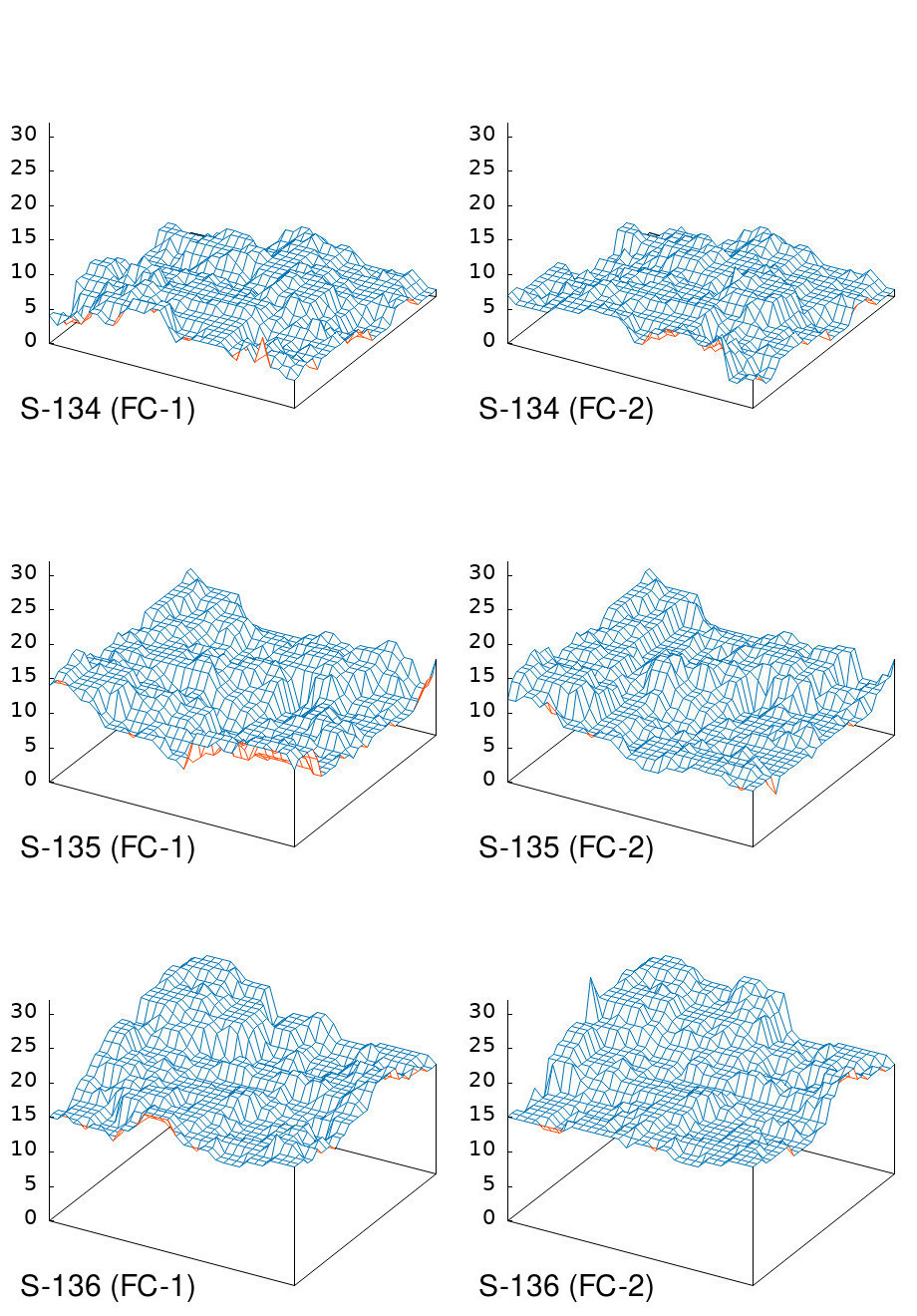
Figure 18: Comparison of fracture surfaces obtained with different fracture criteria. Three different samples are shown, S-134, S-135 and S-136. FC-1 denotes the ’maximum normal stress’ criterion, Eq. (96), and FC-2 denotes the ’maximum shear stress’ criterion, Eq. (89). Fracture interfaces are red on the underside and blue on top.

Brittle fracture on very small scales corresponds to the breaking of atomic bonds, thereby separating crystal planes. The resulting fracture surface is flat until the crack front encounters an obstacle, such as a grain boundary or a lattice defect. On small scales, therefore, it is not unreasonable to expect fracture surfaces akin to those shown on the left in Fig. 15. These were obtained with the ’erroneous’ criterion, Eq. (34), which, while lending much weight to axial force, has only weak contributions from bending and none from shear.

Eq. (34) should, of course, not be regarded as an adequate criterion for brittle fracture on small scales. While the large scale fracture criteria, Eqs. (89) and (96), were derived from the theory of elasticity, a small scale criterion would require an analysis which takes into account the microscopic nature of the structure, such as, for instance, binding by interatomic potentials. From this a relevant functional form could be devised for a fracture criterion to be used in discrete element modeling at small scales. This should lend appropriate weight to the tensile breaking which gives rise to the cleavage process that takes place between crystal planes. At the same time it should include a less dominating mechanism (based on bending or shear or both) that emulates encounters with grain boundaries and other discontinuities within the crystal structure of the material.

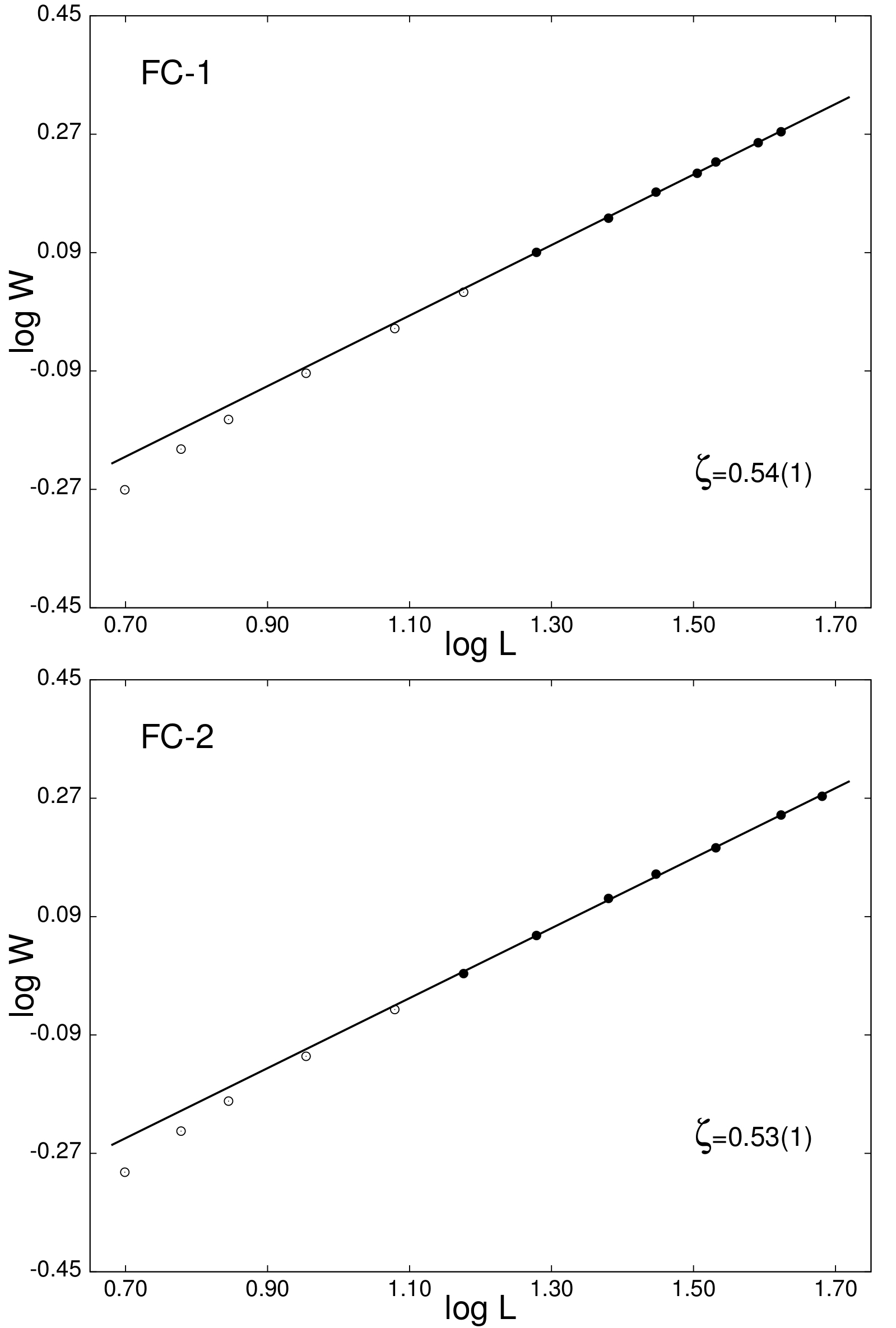
Figure 19: Log-log plots for average roughness, $W$, as a function of system size, $L$, for a large number of fractured samples. Disorder magnitude is $D=2$. Shown at the top (FC-1) is the result obtained with the ’maximum normal stress’ criterion, Eq. (96). Shown below (FC-2) is the result obtained with the ’maximum shear stress’ criterion, Eq. (89).

This picture goes a long way towards explaining why two different exponents are obtained in the experiments. In numerical modeling with an appropriate fracture criterion which includes breaking due to shear, we obtain $\zeta\sim 0.5$ on scales large enough for shear to play an important role. Contarary to this, $\zeta\sim 0.8$ is expected on scales sufficiently small to be dominated by the crystal structure, as indicated by an ’erroneous’ criterion, such as Eq. (34), which lends a disproportionally strong weight to tensile breaking.

In previous calculations with Eq. (34) it was seen that the large scale roughness exponent $\zeta\sim 0.5$ is approached from above when the disorder strength is considerably increased, resulting in $\zeta=0.62$ being obtained for $D=2$ and $\zeta=0.59$ for $D=4$ skj2 . The latter case, however, represents a material structure with quite extreme variations in local strength properties, perhaps unrealistically so for most materials.

It is worth noting that with the new criteria, given by Eqs. (89) and (96), the roughness exponent remains in the vicinity of $\zeta=0.5$ for all disorders included in the present study. In other words, the roughness appears to be universal with respect to disorder strength, in contrast with what was found in Ref. skj2 . With $D=2$ the exponents obtained with Eqs. (89) and (96) are $\zeta=0.54$ and $\zeta=0.53$, respectively. The result is shown in Fig. 19. At $D=3$ we obtain $\zeta=0.53$ with both criteria, this is shown in Fig. 20. Finally, at $D=4$ we obtain $\zeta=0.52$ using Eq. (96), in this case we did not take the

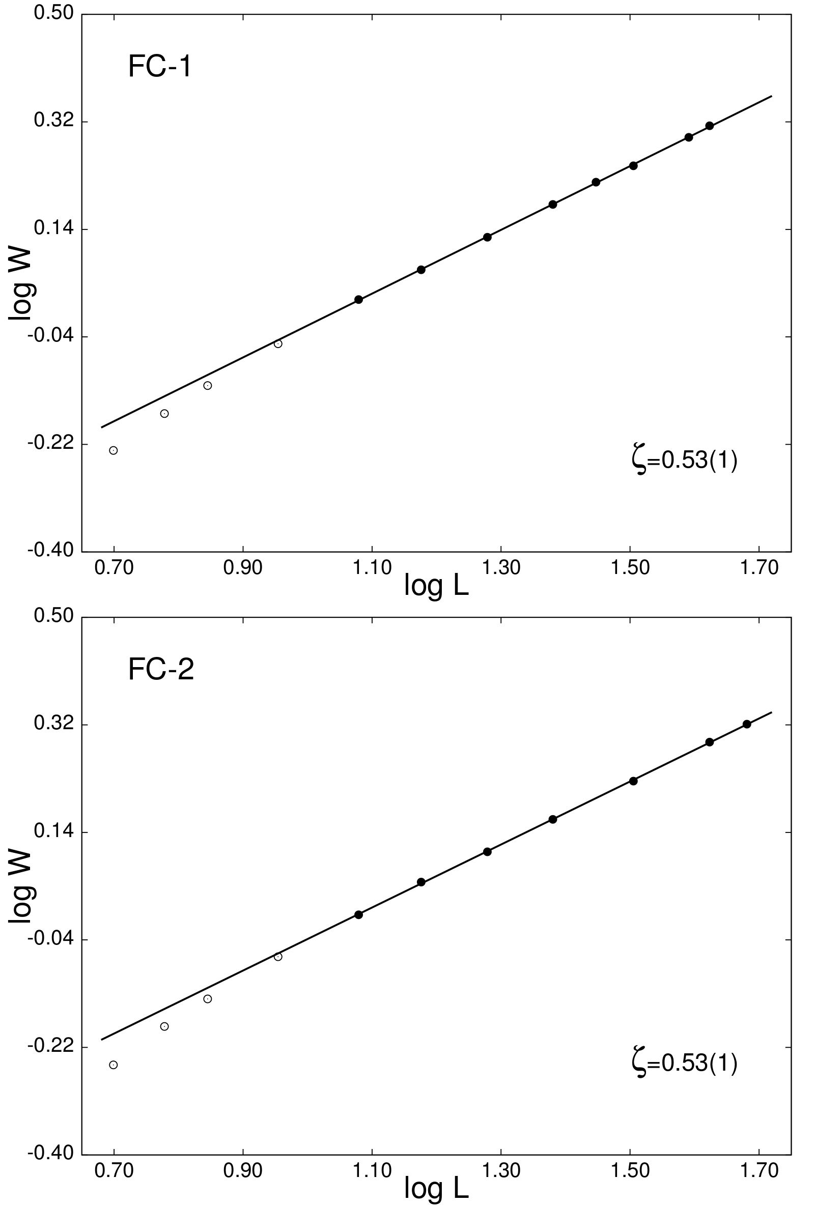
Figure 20: Log-log plots for average roughness, $W$, as a function of system size, $L$, for a large number of fractured samples. Disorder magnitude is $D=3$. Shown at the top (FC-1) is the result obtained with the ’maximum normal stress’ criterion, Eq. (96). Shown below (FC-2) is the result obtained with the ’maximum shear stress’ criterion, Eq. (89).

trouble to run an extra set of simulations for Eq. (89). The result is shown in Fig. 21. The apparently constant value which, within the uncertainties of the straight-line fit, seems to fit all disorder strengths currently investigated with new fracture criteria is $\zeta=0.53$.

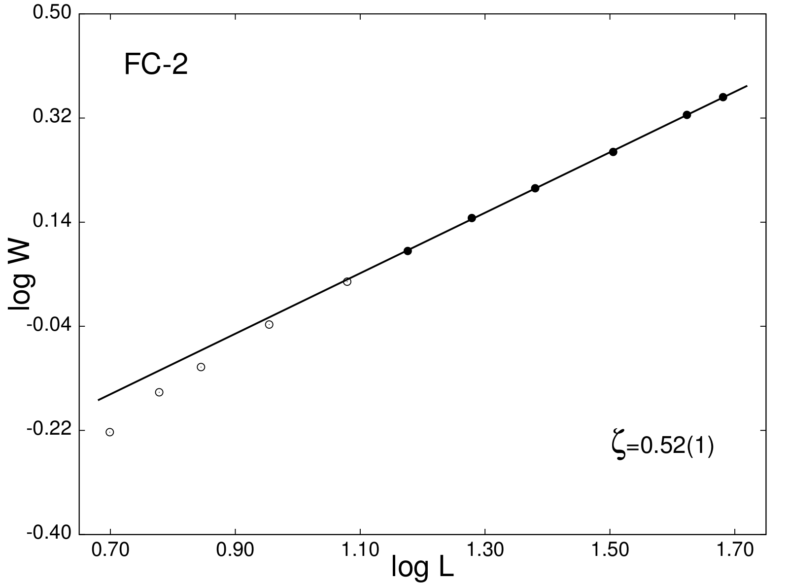
Figure 21: Log-log plot showing average roughness, $W$, as a function of system size, $L$, for a large number of fractured samples of each size. Disorder magnitude is $D=4$ and FC-2 denotes the result obtained with the ’original’ fracture criterion, Eq. (34).

VII Externally Applied Torque on a Cylindrical Shaft

A typical property of brittle materials is that they are stronger in shear than in tension. As such, the criterion given by Eq. (34) does capture one essential feature of brittle fracture, namely the preference towards failure in axially tensile loading. If this was the only requirement a fracture criterion even more simple than Eq. (34) might have been sufficient, e.g., one that contains a single term only – the ratio of the axial load to the failure load.

In discrete element modeling there is, however, another feature which influences crack propagation and, ultimately, crack morphology: the geometry of the lattice discretization. Our current model is a cube lattice with nodes arranged as shown in Fig. 1. For a crack to propagate obliquely with respect to the alignment of ’beams’, breaks will have to occur by lateral (transverse) deformation as well as by longitudinal (axial) deformation. For a cube lattice strained in the $Z$-direction lateral breaks are those that occur within the $XY$-plane due to deformations transverse to the ’beam’ axis, i.e., shear deformations normal to (or bending deformations out of) this plane. In other words, a fracture plane which intersects the $XZ$-plane at an angle of exactly 45 degrees will require an equal number of transverse and longitudinal breaks. In localized fracture (very weak or no disorder) these two types of breaking events should alternate as the line of intersection between the crack front and the $XZ$-plane advances.

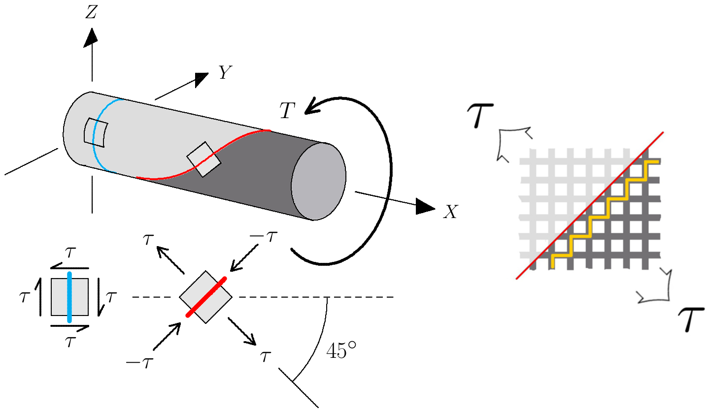
Figure 22: A positive valued torque $T$ is applied on the right end of a cylindrical shaft, with the left end being held fixed. Shown in blue is an intersecting plane on which the shear stresses are at their highest. The associated material element is one of pure shear, with the largest values obtained vertically or horizontally. Shown in red is an intersecting helical surface perpendicular to which tensile forces are highest. The associated material element indicates the direction and value of the maximum tensile and compressive normal stresses. This element is contained within the lattice discretization on the right, with a numerical realization of the helical surface depicted in yellow.

For a fracture plane which advances at a steeper angle, the ratio of horizontal to vertical breaks increases, while a more shallow fracture plane likewise requires relatively fewer horizontal breaks.

Without providing for the possibility of shear failure, crack propagation would instead display a preference towards either the vertical or the horizonal plane, depending on the direction of the external loading. A situation requiring propagation along a plane inclined at 45 degrees is the fracture of a cylindrical shaft due to torque, see Fig. 22. Directional inhomogeneity in the elastic properties of the cylinder (other than disorder) could modify the angle of the fracture surface, but in the case of a shaft with homogeneous material properties the emerging fracture angle should be 45 degrees in brittle fracture. Any deviation from this should instead be obtained by controlling the strength ratio of shear to tension in the thresholds. For a discrete element model such a freedom of choice is essential in order to obtain a crack which correctly reflects both the underlying structural disorder as well as other assumed material properties.

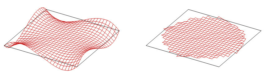
Figure 23: Mid-point sections in a body subject to torsion. On the left is a square cross-section, showing the characteristic out-of-plane warping obtained for non-circular cross-sections. On the right is a circular cross-section obtained by cutting beams outside a circle inscribed within the square. Vertical displacements have been magnified by a factor of 50.

We therefore next compare the new fracture criteria with the old criterion by considering torsional fracture in a cylindrical shaft. To construct such an object we first regard a rectangular column of discrete element ’beams’ using the cube lattice discretization. From this a cylindrical body is obtained by inscribing a circle within the limits of the square cross-section, before cutting away all discrete elements connected to nodes lying outside this circle. This is shown in Fig. 23, for a structure subject to external torque. On the left the characteristic out-of-plane warping of non-circular cross sections is shown for a square cross-section in the $XY$-plane,

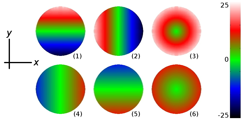
Figure 24: Stresses on the central cross-section of a cylinder subjected to an external torque. Shown are stresses in discrete element ’beams’ which connect horizontal layers in the cylinder, i.e., ’beam’ $6$ in Fig. 1. Shear stresses are displayed at the top and bending stresses at the bottom. See main text for more information.

while on the right a circular cross-section is shown. The amount of torsion involved is the same in both cases, and the vertical displacements have been exaggerated by a factor of fifty. Although it is unlikely that the warping of the square cross-section influences the nature of the fracture surface, we only consider circular cross-sections in the following. (The very minimal slanting seen at some of the edges of the circular cross-section on the left in Fig. 23 are probably finite-size lattice effects.)

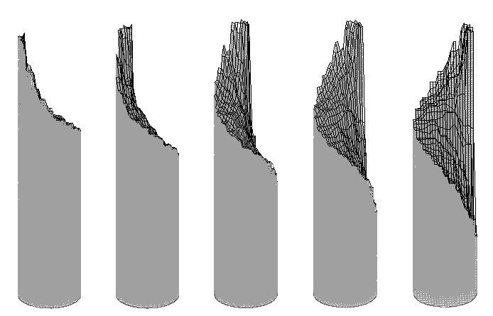
Figure 25: A cylindrical shaft with diameter $d=25$ and height $H=201$ which has been broken on the application of torque. The fracture criterion used is Eq. (34). The shaft is shown from five slightly different angles.

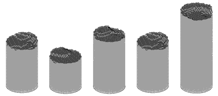
Figure 26: Cylindrical shafts with diameter $d=25$ and height $H=101$ broken by the application of torque. The fracture criterion used is Eq. (96), where tensile thresholds are twice as large as shear thresholds. Five different samples have been shown here.

Shear and bending stresses on the cross-section of a cylindrical shaft induced by torque is shown in Fig. 24. At the top, (1) and (2) displays $X_{6}$ and $Y_{6}$, i.e., shear forces in the $X$- and $Y$-directions. These are obtained from the $j=6$ components of Eqs. (27) and (28), respectively. Also shown, (3) is

$$V_{xy}=\sqrt{X_{6}^{2}+Y_{6}^{2}},$$ (104)

i.e., the bi-planar shear of Eq. (93). Below the shear stresses are shown bending stresses. These, (4) and (5), are $V_{6}$ and $U_{6}$, respectively. Also, (6) represents

$$M_{xy}=\sqrt{V_{6}^{2}+U_{6}^{2}},$$ (105)

or the bi-axial bending moment of Eq. (95). This combines bending within the $XZ$- and $YZ$-planes. Fig. 24 shows that (with Eqs. (14 and (15) for the elastic constants) shear stresses are about twice as large as bending stresses. The necessity of using Eqs. (104) and (105) for consistency with rotational symmetry is also apparent.

Using the old criterion, Eq. (34), a typical example of the helical fracture surfaces obtained is shown from five slightly different angles of rotation in Fig. 25. The sample has been subjected to a counter-clockwise rotation at the top and a clockwise rotation at the bottom. All samples considered currently have weak disorder, i.e., using $D=0.4$ in Eq. (33). What is immediately apparent is that the angle of the fracture surface is rather steep. This is a reflection on the fact that Eq. (34) is dominated by a purely axial term while having only a weak contribution from bending. It is this bending which provides the first local fractures since the main forces are due to displacements transverse to the vertical axis. At some point, however, breaking due to horizontal tension becomes important. Crack propagation in the form of separation along vertical lattice planes now becomes more dominant than breaking induced by bending within the horizontal plane. The resulting fracture surfaces tend to be very steep, significantly exceeding the 45 degree angle in Fig. 22, as is evident in Fig. 25.

Figure 27: Cylindrical shafts with diameter $d=25$ and height $H=101$ broken by the application of torque. The fracture criterion used is Eq. (96), where tensile and shear thresholds are equal. Five different samples are shown.

Figure 28: Cylindrical shafts with diameter $d=25$ and height $H=101$ broken by the application of torque. The fracture criterion used is Eq. (96), where shear thresholds are one and a half times as strong as tensile thresholds. The samples have been rotated to display more or less the same view.

If instead we use our new criterion, Eq. (96), we have the option to vary the strength relationship between shear and tension. Assuming the material is stronger in tension than in shear we should expect ’flat’ fracture surfaces. Indeed, fracture surfaces obtained for a shear/tension ratio of $0.5$ are quite flat and five samples are shown in Fig. 26. Such a strength ratio is typical of many metals, including steel deut . These materials display less resistance towards the movement of dislocations within crystal planes and are thus more susceptible to failure due to shear deformations.

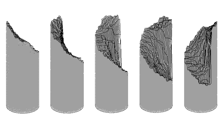
Figure 29: A cylindrical shaft with diameter $d=25$ and height $H=101$ broken by the application of torque. The fracture criterion used is Eq. (96), where shear thresholds are twice as strong as tensile thresholds. A typical sample is shown from five slightly different angles.

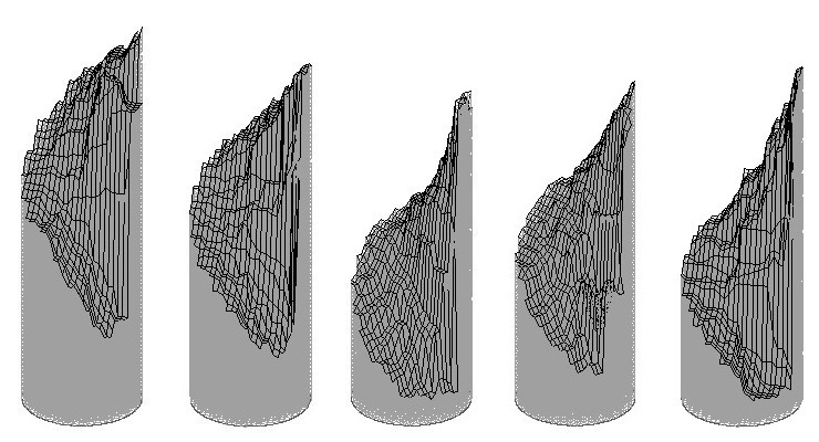
Figure 30: Cylindrical shafts with diameter $d=25$ and height $H=101$ broken by the application of torque. The fracture criterion used is Eq. (96), where shear thresholds are four times as strong as tensile thresholds. The samples have been rotated to display more or less the same view.

Increasing the stochastically generated shear strength to the point where it equals the stochastically generated tensile strength changes the appearance of the fracture surfaces. Some of the samples now display a slanting surface while others are reminiscent of a cup-and-cone type surface (common in ductile fracture), see the five samples in Fig. 27.

Helical fracture surfaces of the type expected in Fig. 22 appear as soon as the shear strength is increased beyond the tensile strength. In Fig. 28 shear is one and a half times stronger than tension, with five typical samples shown. A single sample where shear is twice as strong as tension is shown from five slightly different angles in Fig. 29. Strength ratios where shear is stronger than tension is typical of many rock types jaeg .

Further increase of shear strength relative to tensile strength causes the angle of fracture to become progressively steeper. In Figs. 30 and 31 the ratios are four and eight, respectively.

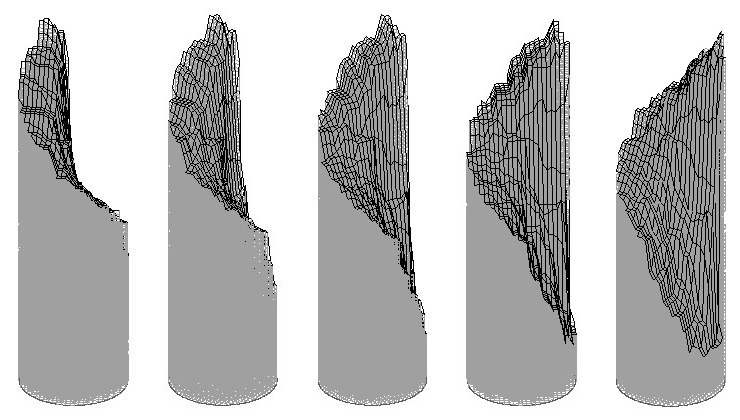
Figure 31: Cylindrical shaft with diameter $d=25$ and height $H=101$ broken by the application of torque. The fracture criterion used is Eq. (96), where shear thresholds are eight times as strong as tensile thresholds. A typical sample shown from five slightly different angles.

Even when compared with these rather extreme cases, however, fracture surfaces obtained with the original criterion, Eq. (34), are even more steep. In fact, they almost traverse the entire length of the sample. Such separation along vertical planes would perhaps be similar to the sort of fracture taking place when a broom stick is twisted until it breaks. Fracture then occurs as a separation of wood fibres that are parallel to the length axis of the shaft, rather than the breaking of such fibres in the direction normal to the axis, as would be expected in shear fracture.

VIII Concluding Remarks

The choice of fracture criterion is shown to have a profound effect on the crack morphology which obtains in calculations with a discrete element model for brittle fracture. The new fracture criteria are based on well known and long established relations and principles from the theory of elasticity, and replace a criterion which is really only relevant to plastic (rather than brittle) fracture. Modes of deformation such as axial strain, bending, shear and torsion are all included in the criteria used.

It is especially the inclusion of shear which most affects the results obtained. Visually, the most conspicuous change is observed at the weak end of the currently included range of disorders. Here the resulting fracture surfaces appear considerably more rough. The way this influences the self-affine properties of the crack is to lower the roughness exponent to a value consistent with experimental findings, i.e., $\zeta=0.52$. What is more, the roughness exponent remains at this value for all disorders currently included, indicating a universal value. An additional gain produced by allowing breaking in other deformation modes, notably shear, is to enable the crack front to move more freely with respect to the lattice topology. Otherwise, for a criterion with an axially dominant breaking mechanism, crack propagation will display a tendency to align itself in parallel with symmetry planes in the lattice. We have used a cube lattice, although this does not strictly reproduce the correct macroscopic response to an external loading. It is, however, less demanding on numerical resources than would be, say, an hexagonal close-packed lattice configuration.

No investigation into how results depend on the chosen elastic constants has been made in this study, this should probably be addressed in a future study.

- (1) Dynamical Theory of Crystal Lattices, M. Bohm, and K. Huang, (Oxford University Press, New York, 1954).
- (2) S. Roux, and E. Guyon, Mechanical percolation : a small beam lattice study, J. Phys. (Paris) Lett. 46, L999 (1985).
- (3) H. J. Herrmann, A. Hansen, and S. Roux, Fracture of disordered, elastic lattices in two dimensions, Phys. Rev. B 39, 637 (1989).
- (4) R. J. Roark, and W. C. Young, Formulas for Stress and Strain, (McGraw-Hill Book Company, New York, 1975).
- (5) S. H. Crandall and N. C. Dahl, An Introduction to the Mechanics of Solids, McGraw-Hill Book Company, New York, 1959.
- (6) M. R. Hestenes and E. Stiefel, Methods of conjugate gradients for solving linear systems, Nat. Bur. Stand. J. Res. 49, 409 (1952).
- (7) W. H. Press, S. A. Teukolsky, W. T. Vetterling and B. P. Flannery, Numerical Recipes in Fortran 77, (Cambridge University Press, New York, 1992).
- (8) B. Skjetne, T. Helle, and A. Hansen, Roughness of crack interfaces in two-dimensional beam lattices, Phys. Rev. Lett. 87, 125503 (2001).
- (9) See, e.g., J. J. Stalnaker and E. C. Harris, Structural Design in Wood, Van Nostrand Reinhold, New York, 1989.
- (10) See, e.g., J. Chakrabarti, Theory of Plasticity, McGraw-Hill Book Company, New York, 1987.
- (11) ANSI/AWC NDS-2015, National Design Specification for Wood Construction, American Wood Council, 2015.
- (12) See, e.g., A. Carpinteri, Structural Mechanics: A Unified Approach, Taylor & Francis Ltd, London, 1997; S. P. Timoshenko, History of Strength of Materials, McGraw-Hill Book Company, New York, 1953.
- (13) P. C. Chou and N. J. Pagano, Elasticity: Tensor, Dyadic, and Engineering Approaches, D. Van Nostrand Company, New York, 1967.
- (14) A. A. Afrouz, Practical Handbook of Rock Mass Classification Systems and Modes of Ground Failure, CRC Press, Boca Raton, Florida, 1992.
- (15) NASA TM X-73305, Astronautic Structures Manual, Volume I, Marshall Space Flight Center, Huntsville, Alabama, August 1975
- (16) B. E. Steeve and R. J. Wingate, NASA/TM 2012-217454, Marshall Space Flight Center, Huntsville, Alabama, March 2012
- (17) B. Skjetne, T. Helle and A. Hansen, Front. Phys. 2:68 (2014).
- (18) B. B. Mandelbrot, D. E. Passoja, and A. J. Paullay, Fractal character of fracture surfaces of metals, Nature (London) 308, 721 (1984).
- (19) E. Bouchaud, Scaling properties of cracks, J. Phys. Condens. Matter 9, 4319 (1997).
- (20) See, e.g., H. J. Herrmann, and S. Roux, Statistical Models for the Fracture of Disordered Media, (North-Holland, Amsterdam, 1990).
- (21) M. J. Alava, P. K. V. V. Nukala, and S. Zapperi, Statistical models of fracture, Adv. Phys. 55, 349 (2006).
- (22) G. G. Batrouni, and A. Hansen, Fracture in three-dimensional fuse networks Phys. Rev. Lett. 80, 325 (1998).
- (23) V. I. Räisänen, M. J. Alava, and R. M. Nieminen, Fracture of three-dimensional fuse networks with quenched disorder, Phys. Rev. B 58, 14288 (1998).
- (24) V. I. Räisänen, E. T. Seppälä, M. J. Alava, and P. M. Duxbury, Quasistatic cracks and minimal energy surfaces Phys. Rev. Lett. 80, 329 (1998).
- (25) P. K. V. V. Nukala, S. Zapperi, and S. Šimunović, Crack surface roughness in three-dimensional random fuse networks, Phys. Rev. E 74, 026105 (2006).
- (26) A. Parisi, G. Caldarelli, and L. Pietronero, Roughness of fracture surfaces, Europhys. Lett. 52, 304 (2000).
- (27) P. K. V. V. Nukala, P. Barai, S. Zapperi, M. J. Alava, and S. Šimunović, Fracture roughness in three-dimensional beam lattice systems, Phys. Rev. E 82, 026103 (2010).
- (28) J. M. Boffa, C. Allain, and J. Hulin, Experimental analysis of fracture rugosity in granular and compact rocks, Eur. Phys. J 2, 281 (1998).
- (29) L. Ponson, H. Auradou, M. Pessel, V. Lazarus, and J. P. Hulin, Failure mechanisms and surface roughness statistics of fractured Fontainebleau sandstone, Phys. Rev. E 76, 036108 (2007).
- (30) See, e.g., A. D. Deutschman, Machine Design: Theory and Practice, Prentice Hall, Lebanon, Indiana, 1975.
- (31) J. C. Jaeger and N. G. W. Cook, Fundamentals of Rock Mechanics, Chapman and Hall Ltd, London, 1979.