Abstract

By starting with a two-fields model in which the fields and their derivatives are nonminimally coupled to gravity, and then by using a conformal gauge, we obtain a model in which the derivatives of the canonically normalized field are nonminimally coupled to gravity. By adopting some appropriate functions, we study two cases with constant and E-model nonminimal derivative coupling, while the potential in both cases is chosen to be E-model one. We show that in contrary to the single field $\alpha$-attractor model that there is an attractor point in the large $N$ and small $\alpha$ limits, in our setup and for both mentioned cases there is an attractor line in these limits that the $r-n_{s}$ trajectories tend to. By studying the linear and nonlinear perturbations in this setup and comparing the numerical results with Planck2015 observational data, we obtain some constraints on the free parameter $\alpha$. We show that by considering the E-model potential and coupling function, the model is observationally viable for all values of $M$ (mass scale of the model). We use the observational constraints on the tensor-to-scalar ratio and the consistency relation to obtain some constraints on the sound speed of the perturbations in this model. As a result, we show that in a nonminimal derivative $\alpha$-attractor model, it is possible to have small sound speed and therefore large non-Gaussianity.
PACS: 98.80.Cq , 98.80.Es
Key Words: Cosmological Perturbations, Non-Gaussianity, Nonminimal Derivative Coupling, $\alpha$-Attractor, Observational Constraints.

1 Introduction

Considering a single canonical scalar field (inflaton) responsible for cosmological inflation in early universe, is a simplest way to solve some problems of the standard model of cosmology. To have enough e-folds number or equivalently enough exponential expansion of the universe, the inflaton should rolls slowly down toward the minimum of its potential. In this simple inflation model, an adiabatic, scale invariant and gaussian mode of the primordial perturbations is dominant [1, 2, 3, 4, 5, 6, 7, 8, 9]. However, it seems that in the future, with the advancement of technology, we should be able to detect the non-Gaussian distributed modes of the perturbations. Also, some extended models of inflation predict scale dependent and non-Gaussian features of the primordial perturbations [9, 10, 11, 13, 14, 15, 16, 17, 18]. In this regard, in studying the inflation, the models predicting the non-Gaussian perturbations are really interesting.

It is possible the scalar field responsible for cosmological inflation to be the Higgs boson. It is proposed that to adopt the Higgs boson as the inflaton, we should consider a nonminimal coupling between its derivatives and Einstein tensor [19, 20]. In this case, the friction is enhanced gravitationally at higher energies because of the presence of nonminimal derivative coupling. This means that the friction of an inflaton rolling down its own potential increases significantly, allowing occurrence of the slow-roll inflation even with steep potentials. The models with nonminimal derivatives coupling are capable to solve the unitary violation problem during inflation. In these models, unitarity is not violated up to the quantum gravity scales and also, quantum gravity regime is avoided during Inflation [20, 21]. Note that, in [20] it has been shown that to trust the effective inflationary description, the curvature should be much smaller than the Planck scale. Considering the relation $R=6(\dot{H}+2H^{2})$ and the fact that during inflation era $H$ is nearly constant and $\dot{H}$ is very small, we have $R\simeq 12H^{2}$. So we can say that, to avoid the unitarity problem during inflation, $H$ should be much smaller than Planck mass and this is the unitarity bound. In the nonminimal derivative model this bound is not violated [20, 21, 22]. Also, in these models the perturbations are somewhat scale dependent and it is possible to have non-Gaussian distributed perturbations. We refer to [23, 24, 25, 26] for some works on the issue of nonminimal derivatives in the early time accelerating expansion of the universe as well as the late time cosmic dynamics.

Recently, the idea of “cosmological attractor” in the models describing the cosmological inflation has attracted a lot of attention. The conformal attractors [27, 28] and $\alpha$-attractors [29, 30, 31, 32] models are some models which incorporates the idea of the cosmological attractors. In Refs. [33, 34, 35, 36, 37, 38, 39, 40, 41, 42] some more details on the issue of $\alpha$-attractors have been studied. The conformal attractor model has the universal prediction in the large e-folds number ($N$) for the scalar spectral index and tensor-to-scalar ratio as $n_{s}=1-\frac{2}{N}$ and $r=\frac{12}{N^{2}}$, respectively. The $\alpha$-attractor models are divided into two categories named E-model and T-model, according to the adopted potentials. The E-model corresponds to the following potential

$$V=V_{0}\Big{[}1-\exp\big{(}-\sqrt{\frac{2\kappa^{2}}{3\alpha}}\phi\big{)}\Big{]}^{2n}\,,$$ (1)

and the T-model is characterized by a potential as

$$V=V_{0}\tanh^{2n}\Big{(}\frac{\kappa\phi}{\sqrt{6\alpha}}\Big{)}\,.$$ (2)

In these potentials, $V_{0}$, $n$ and $\alpha$ are some free parameters. The prediction of the scalar spectral index in the $\alpha$-attractor model is similar to the prediction in the conformal attractor ones as $n_{s}=1-\frac{2}{N}$ in small $\alpha$ and large $N$ limits. However, it predicts the tensor-to-scalar ratio as $r=\frac{12\alpha}{N^{2}}$ in small $\alpha$ and large $N$ limits, which is somewhat different from the one predicted by the conformal attractor model.

In this paper, we are going to study a nonminimal derivatives model in which both the potential and nonminimal derivatives coupling function are E-model type. Actually, the author of Ref. [23] has studied the nonminimal derivatives model in which the coupling function is a constant. He has adopted several types of potential such as $\phi^{2}$, $\phi^{4}$, exponential and so on. Our attention here is on $\phi^{2}$ potential. In Ref. [23], it has been shown also that the nonminimal derivatives model with $\phi^{2}$ potential is consistent with joint data of WMAP7 [43], BAO [44], and HST [45] for $N=50$, $60$ and $70$. However, if we compare the results with Planck2015 TT, TE, EE+lowP data [46] the model is observationally viable just for some values of $M$ (the mass scale of the nonminimal derivative coupling). We are going to check that by considering E-type potential and coupling function, whether the numerical results of the model are consistent with Planck2015 TT, TE, EE+lowP data background for all values of $M$ or not. In this regard, we follow Refs. [27, 28] and consider a model with two real scalar fields $\psi$ and $\varphi$. The nonminimal action written in Ref. [27] is conformal invariant. The authors in this reference have used a $SO(1,1)$ conformal gauge (named rapidity gauge) as

$$\psi^{2}-\varphi^{2}=6$$ (3)

which represents a hyperbola. By using a canonically normalized field as

$$\psi=\sqrt{6}\cosh(\frac{\phi}{\sqrt{6}})\,\,,\quad\varphi=\sqrt{6}\sinh(\frac{\phi}{\sqrt{6}})$$ (4)

they were able to eliminate the nonminimal terms in the action and transform the nonminimal action to the minimal one accordingly. Actually, by adopting several types of the potential terms, they have obtained the models corresponding to dS/AdS space, T-model of chaotic inflation and Starobinsky model of inflation [47, 48, 49].

In our setup, both the fields and their derivatives are nonminimally coupled to gravity. To eliminate the nonminimal coupling ( not the “nonminimal derivatives coupling”) we use the gauge (3) and also rewrite equation (4) as

$$\psi=\sqrt{6}\cosh(\frac{\phi}{\sqrt{6\alpha}})\,\,,\quad\varphi=\sqrt{6}\sinh(\frac{\phi}{\sqrt{6\alpha}})$$ (5)

where the free parameter $\alpha$ has been included which leads us to E-model $\alpha$-attractor. Actually, $\alpha$ is inversely proportional to the curvature of the inflaton Kähler manifold [31]. By using this field, we re-parameterize the two fields model and convert it to a one-filed model with nonminimal derivatives coupling shown by the function ${\cal{F}}$. We study two cases as ${\cal{F}}=const.$ and ${\cal{F}}={\cal{F}}(\phi)$ and then we study cosmological inflation and perturbations in this setup. We show that in both cases there is an attractor line in large $N$ and small $\alpha$ limits which the $r-n_{s}$ trajectories tend to. Note that, as we said, in the the single field $\alpha$-attractor model there is an attractor point in these limits. In Ref. [50] it has been shown that in the Gauss-Bonnet $\alpha$-attractor model also, there is an attractor point in the mentioned limits. Indeed, the presence of line instead of point is because of considering the nonminimal derivatives coupling which causes the scalar spectral index of this model to be a functions of $\alpha$ and $M$. For $M\rightarrow\infty$, we recover the attractor point in usual $\alpha$-attractor models.

In section 2, we study the inflation in this NMDC $\alpha$-attractor model and obtain the background equations of the model. In section 3, by using the ADM formalism, we study the linear perturbations in this model. In this section, we obtain some expressions for the scalar spectral index and tensor-to-scalar ratio and compare the results with Planck2015 observational data to test the observational viability of the model. In this regard, we obtain some constraints on parameter $\alpha$. In section 4, we study the non-linear perturbations and non-Gaussian features of the primordial perturbations. By using the relations between the tensor-to-scalar ratio and sound speed, and using the allowed values of the tensor-to-scalar ratio (from $95\%$ CL of Planck2015 TT, TE, EE+lowP data), we obtain constraints on the sound speed in this model. These constraints show that it is possible to have large non-Gaussianity in this model. In section 5 we present a summary of our work.

2 Inflation

The action of a model with two real scalar fields $\psi$ and $\varphi$, with both nonminimal and nonminimal derivatives couplings to the gravity, is given by

$$S=\int d^{4}x\sqrt{-g}\Bigg{[}\frac{\psi^{2}}{12\kappa^{2}}R+\frac{1}{2}\partial_{\mu}\psi\,\partial^{\mu}\psi-\frac{\varphi^{2}}{12\kappa^{2}}R-\frac{1}{2}\partial_{\mu}\varphi\,\partial^{\mu}\varphi+\frac{1}{2M^{2}}\,f\,G^{\mu\nu}\partial_{\mu}\psi\,\partial^{\mu}\psi$$

$$-\frac{1}{2M^{2}}\,F\,G^{\mu\nu}\partial_{\mu}\varphi\,\partial^{\mu}\varphi-U(\psi,\varphi)\Bigg{]},$$ (6)

where the functions $f$ and $F$ show the nonminimal derivatives coupling and are functions of the corresponding scalar field. Also, $U$ is a potential term which is a function of the scalar fields. In the absence of nonminimal derivatives coupling, the theory is conformally invariant and by using the gauge $\psi^{2}-\varphi^{2}=6$ can be converted to the minimal coupling case [30]. The action (2) by nonminimal derivatives coupling is a disformally invariant action [51]. Now, to proceed, we should specify all three functions $f$, $F$ and $U$. We can adopt the nonminimal derivatives coupling functions similar to the nonminimal coupling ones as $f=\psi^{2}$ and $F=\varphi^{2}$. However, by this choice, if we use gauge (3) the nonminimal derivatives term vanishes (note that, we use this gauge to eliminate the effect of nonminimal coupling). We are not interested to this case because our aim in this paper is to study the nonminimal derivatives model. So, we put this case aside. On the other hand, since we seek for the effects of the free parameter $\alpha$ on the observational viability of nonminimal derivatives model by E-model potential and coupling function, we should choose $f$ and $F$ in the way satisfying our purpose. In another words, we should adopt appropriate functions so that after using the gauge (3) we reach a nonminimal derivatives function with E-model type of the scalar field’s functions. To cover this purpose, it is convenient to consider the same interacting function for $f$ and $F$ as $f=F=\hat{{\cal{F}}}(\psi,\varphi)$. Now, by using the definitions in equation (5), we obtain

$$\frac{\psi^{2}}{12}-\frac{\varphi^{2}}{12}=\frac{1}{2}\,,$$ (7)

and

$$\partial_{\mu}\psi\,\partial^{\mu}\psi-\partial_{\mu}\varphi\,\partial^{\mu}\varphi=\partial_{\mu}\phi\,\partial^{\mu}\phi\,.$$ (8)

We also define $\hat{{\cal{F}}}(\psi,\varphi)={\cal{F}}(\phi)$ and $U(\psi,\varphi)=V(\phi)$. Now, we can rewrite the action (2) in the following form

$$S=\int d^{4}x\sqrt{-g}\Bigg{[}\frac{1}{2\kappa^{2}}R+\frac{1}{2}\partial_{\mu}\phi\,\partial^{\mu}\phi+\frac{1}{2M^{2}}{\cal{F}}(\phi)G^{\mu\nu}\partial_{\mu}\phi\,\partial^{\mu}\phi-V(\phi)\Bigg{]},$$ (9)

In a spatially flat FRW metric, the action (9) leads to the following Friedmann equation

$$H^{2}=\frac{\kappa^{2}}{3}\left[\frac{\dot{\phi}^{2}}{2}\Big{(}1-\frac{9}{M^{2}}H^{2}{\cal{F}}\Big{)}+V(\phi)\right],$$ (10)

where, a dot denotes a time derivative of the parameter. Variation of the action (9) with respect to the scalar field, gives the equation of motion of the field $\phi$ as follows

$$\ddot{\phi}\Big{(}-1+3\frac{{\cal{F}}H^{2}}{M^{2}}\Big{)}+\Big{(}\frac{6}{M^{2}}{\cal{F}}H\dot{H}+\frac{9}{M^{2}}{\cal{F}}H^{3}-3H\Big{)}\dot{\phi}+6{\cal{F}}^{\prime}H^{2}\dot{\phi}^{2}-V^{\prime}=0\,,$$ (11)

where, a prime refers to a field derivative of the parameter. Considering the definitions $\epsilon=-\frac{\dot{H}}{H^{2}}$ and $\eta=-\frac{1}{H}\frac{\ddot{H}}{\dot{H}}$, we obtain the slow-roll parameters in our setup as

$$\epsilon=\frac{Y}{1+\frac{\kappa^{2}}{2M^{2}}{\cal{F}}\dot{\phi}^{2}},$$ (12)

$$\eta=2\epsilon-\frac{\dot{Y}}{H\epsilon(1+\frac{\kappa^{2}}{2M^{2}}{\cal{F}}\dot{\phi}^{2})}+\frac{Y}{H\epsilon}\frac{\kappa^{2}{\cal{F}}^{\prime}\dot{\phi}^{3}+2\kappa^{2}{\cal{F}}\ddot{\phi}\dot{\phi}}{2M^{2}(1+\frac{\kappa^{2}}{2M^{2}}{\cal{F}}\dot{\phi}^{2})^{2}}\,,$$ (13)

where parameter $Y$ is defined as

$$Y\equiv\frac{\kappa^{2}{\cal{F}}\dot{\phi}\ddot{\phi}}{M^{2}H}+\frac{V^{\prime 2}}{2\kappa^{2}V^{2}}-3\frac{\kappa^{2}{\cal{F}}\dot{\phi}^{2}}{2M^{2}}+\frac{\kappa^{2}{\cal{F}}^{\prime}\dot{\phi}^{3}}{4M^{2}H}\,.\hskip 14.22636pt$$ (14)

To have inflation phase, the slow roll parameters should satisfy the conditions $\epsilon\ll 1$ and $\eta\ll 1$. As soon as one of the slow-roll parameter meets unity, the inflation ends. Satisfying the conditions $\epsilon\ll 1$ and $\eta\ll 1$ means that the conditions $\dot{\phi}^{2}\ll 1$, $\ddot{\phi}\ll 3H\dot{\phi}$, $\frac{9H^{2}|{\cal{F}}|}{2M^{2}}\dot{\phi}^{2}\ll V$ and $|\dot{{\cal{F}}}|\ll|3{\cal{F}}H|$ should be satisfied.

In the inflation era, the Universe expands exponentially. This expansion is characterized by the e-folds number defined as

$$N=\int_{t_{hc}}^{t_{end}}Hdt\,,$$ (15)

where the subscripts $hc$ and $end$ denote the horizon crossing and end of inflation respectively. In our setup, we find

$$N\simeq\int_{\phi_{hc}}^{\phi_{end}}\frac{3H^{2}\Big{(}\frac{3{\cal{F}}H^{2}}{M^{2}}-1\Big{)}}{V^{\prime}}d\phi\,.$$ (16)

In the next section, we study the linear perturbations in the NMDC setup to obtain the important perturbation parameters and compare to the observational data.

3 Linear Perturbations

To study cosmological perturbations in this setup, we use the following ADM perturbed line element

$$ds^{2}=-(1+2{\cal{R}})dt^{2}+2a(t){\cal{D}}_{i}\,dt\,dx^{i}+a^{2}(t)\left[(1-2{\Phi})\delta_{ij}+2{\Theta}_{ij}\right]dx^{i}dx^{j}\,,$$ (17)

where ${\cal{D}}^{i}=\delta^{ij}\partial_{j}{\cal{D}}+v^{i}$. ${\cal{R}}$ and ${\cal{D}}$ are 3-scalars. Also, the vector $v^{i}$ satisfies the condition $v^{i}_{,i}=0$ [52, 53]. The spatial symmetric and traceless shear 3-tensor is denoted by ${\Theta}_{ij}$ and the spatial curvature perturbation is shown by $\Phi$. Here, we consider the scalar part of the the perturbations at the linear level and within the uniform-field gauge ($\delta\phi=0$), as

$$ds^{2}=-(1+2{\cal{R}})dt^{2}+2a(t){\cal{D}}_{,i}\,dt\,dx^{i}+a^{2}(t)(1-2{\Phi})\delta_{ij}dx^{i}dx^{j}\,,$$ (18)

to study the scalar perturbations. Using this perturbed metric and expanding the action (9) up to the second order in perturbations gives the following quadratic action

$$S_{2}=\int dt\,d^{3}x\,a^{3}{\cal{W}}\left[\dot{\Phi}^{2}-\frac{c_{s}^{2}}{a^{2}}(\partial{\Phi})^{2}\right],$$ (19)

where

$${\cal{W}}=-4\frac{\left(\kappa^{-2}+\frac{\dot{\phi}^{2}{\cal{F}}}{2M^{2}}\right)^{2}\left(9\kappa^{-2}H^{2}-\frac{3}{2}\dot{\phi}^{2}+\frac{27H^{2}\dot{\phi}^{2}{\cal{F}}}{M^{2}}\right)}{3\left(2\kappa^{-2}H+\frac{3H\dot{\phi}^{2}{\cal{F}}}{M^{2}}\right)^{2}}+3\left(\kappa^{-2}+\frac{\dot{\phi}^{2}{\cal{F}}}{2M^{2}}\right),$$ (20)

and

$$c_{s}^{2}=3\Bigg{[}2\Big{(}2\kappa^{-2}H+\frac{3H\dot{\phi}^{2}{\cal{F}}}{M^{2}}\Big{)}\Big{(}\kappa^{-2}+\frac{\dot{\phi}^{2}{\cal{F}}}{2M^{2}}\Big{)}H-\Big{(}2\kappa^{-2}H+\frac{3H\dot{\phi}^{2}{\cal{F}}}{M^{2}}\Big{)}^{2}\frac{\kappa^{-2}-\frac{\dot{\phi}^{2}{\cal{F}}}{2M^{2}}}{\kappa^{-2}+\frac{\dot{\phi}^{2}{\cal{F}}}{2M^{2}}}$$

$$+4\Big{(}2\kappa^{-2}H+\frac{3H\dot{\phi}^{2}{\cal{F}}}{M^{2}}\Big{)}\frac{d\Big{(}\kappa^{-2}+\frac{\dot{\phi}^{2}{\cal{F}}}{2M^{2}}\Big{)}}{dt}-2\Big{(}\kappa^{-2}+\frac{\dot{\phi}^{2}{\cal{F}}^{\prime}}{2M^{2}}\Big{)}\,\frac{d(2\kappa^{-2}H+\frac{3H\dot{\phi}^{2}{\cal{F}}}{M^{2}})}{dt}\Bigg{]}$$

$$\Bigg{[}\Bigg{(}9\Big{(}2\kappa^{-2}H+\frac{3H\dot{\phi}^{2}{\cal{F}}}{M^{2}}\Big{)}^{2}-4\Big{(}\kappa^{-2}+\frac{\dot{\phi}^{2}{\cal{F}}}{2M^{2}}\Big{)}\Big{(}9\kappa^{-2}H^{2}-\frac{3}{2}\dot{\phi}^{2}+\frac{27H^{2}\dot{\phi}^{2}{\cal{F}}}{M^{2}}\Big{)}\Bigg{)}\Bigg{]}^{-1}\,.$$ (21)

The parameter $c_{s}^{2}$ is the squared sound speed. We note that in the case of ${\cal{F}}=0$ we recover the standard second order action [9, 11, 12]. The two-point correlation function, which is used to survey the power spectrum of the perturbations, is defined as

$$\langle 0|{\Phi}(0,\textbf{k}_{1}){\Phi}(0,\textbf{k}_{2})|0\rangle=(2\pi)^{3}\delta^{(3)}(\textbf{k}_{1}+\textbf{k}_{2})\frac{2\pi^{2}}{k^{3}}{\cal{A}}_{s}\,.$$ (22)

The parameter ${\cal{A}}_{s}$ in the right hand side of the above equation is dubbed the power spectrum and is given by

$${\cal{A}}_{s}=\frac{H^{2}}{8\pi^{2}{\cal{W}}c_{s}^{3}}\,.$$ (23)

An interesting parameter in studying the scalar perturbations is the scalar spectral index of the primordial perturbations. This parameter specifies the scale dependence of the perturbation. The scalar spectral index is defined as

$$n_{s}-1=\frac{d\ln{\cal{A}}_{s}}{d\ln k}\Bigg{|}_{c_{s}k=aH}=-2\epsilon-\frac{1}{H}\frac{d\ln\epsilon}{dt}-\frac{1}{H}\frac{d\ln c_{s}}{dt}\,.\hskip 28.45274pt$$ (24)

To study tensorial perturbations, by considering the tensor part of the perturbed metric (17) we write the 3-tensor ${\Theta}_{ij}$ as

$${\Theta}_{ij}={\Theta}_{+}\vartheta_{ij}^{+}+{\Theta}_{\times}\vartheta_{ij}^{\times},$$ (25)

with two polarization tensors $\vartheta_{ij}^{(+,\times)}$ satisfying the reality and normalization conditions [13, 14]. The tensor part of the perturbed metric gives the following expression for the second order action for the tensor mode

$$S_{T}=\int dt\,d^{3}x\,a^{3}{\cal{W}}_{T}\left[\dot{\Theta}_{+}^{2}-\frac{c_{T}^{2}}{a^{2}}(\partial{\Theta}_{+})^{2}+\dot{\Theta}_{\times}^{2}-\frac{c_{T}^{2}}{a^{2}}(\partial{\Theta}_{\times})^{2}\right],$$ (26)

where the parameters ${\cal{W}}_{T}$ and $c_{T}^{2}$ are defined as

$${\cal{W}}_{T}=\frac{1}{4\kappa^{2}}\left(1+\frac{\kappa^{2}{\cal{F}}\dot{\phi}^{2}}{2M^{2}}\right),$$ (27)

$$c_{T}^{2}=1-\frac{\kappa^{2}{\cal{F}}\dot{\phi}^{2}}{2M^{2}}\,.$$ (28)

By following the method used in the scalar part, we achieve the following expression for the amplitude of the tensor perturbations

$${\cal{A}}_{T}=\frac{H^{2}}{2\pi^{2}{\cal{W}}_{T}c_{T}^{3}}.$$ (29)

By using equations (27)-(29), we find the tensor spectral index in this setup as

$$n_{T}=\frac{d\ln{\cal{A}}_{T}}{d\ln k}=-2\epsilon\,.$$ (30)

The ratio of the amplitudes of the tensor mode versus the scalar mode, the tensor-to-scalar ratio, is given by

$$r=\frac{{\cal{A}}_{T}}{{\cal{A}}_{s}}\simeq 16c_{s}\epsilon.$$ (31)

Up to this point we have obtained some linear perturbation parameters. Performing a numerical analysis on these parameters gives some perspective on the cosmological viability of the model. In this regard, we should specify the general functions ${\cal{F}}$ and $V$. Following [27, 28], we define $U(\psi,\varphi)$ as follows

$$U(\psi,\varphi)=\frac{\lambda}{4}\varphi^{2}(\varphi-\psi)^{2}$$ (32)

which by using equation (5) leads to

$$V(\phi)=C\left[1-\exp\Bigg{(}-\sqrt{\frac{2\kappa^{2}}{3\alpha}}\,\phi\Bigg{)}\right]^{2}$$ (33)

which is the E-model potential. As we have stated previously, $\alpha$ is inversely proportional to the curvature of the inflaton Kähler manifold. Given that we want to study two cases as ${\cal{F}}=const.$ and ${\cal{F}}={\cal{F}}(\phi)$, we should define two types of function for $\hat{{\cal{F}}}(\psi,\varphi)$. The first one is as

$$\hat{{\cal{F}}}(\psi,\varphi)=\frac{\lambda}{4}(\varphi^{2}-\psi^{2})^{2}$$ (34)

leading to

$${\cal{F}}=9\lambda$$ (35)

This means that by this type of $\hat{{\cal{F}}}(\psi,\varphi)$ and potential defined by (33), we have an inflation model in which the NMDC coupling is constant and potential is E-model. Another function which we consider for $\hat{{\cal{F}}}(\psi,\varphi)$ is defined as

$$\hat{{\cal{F}}}(\psi,\varphi)=\frac{\lambda}{4}\varphi^{2}(\varphi-\psi)^{2}$$ (36)

leading to

$${\cal{F}}(\phi)=C\left[1-\exp\Bigg{(}-\sqrt{\frac{2\kappa^{2}}{3\alpha}}\,\phi\Bigg{)}\right]^{2}\,.$$ (37)

where

$$C=\frac{9\lambda}{4}$$ (38)

By this function and potential (33) we have an inflation model in which both the NMDC function and potential are E-model.

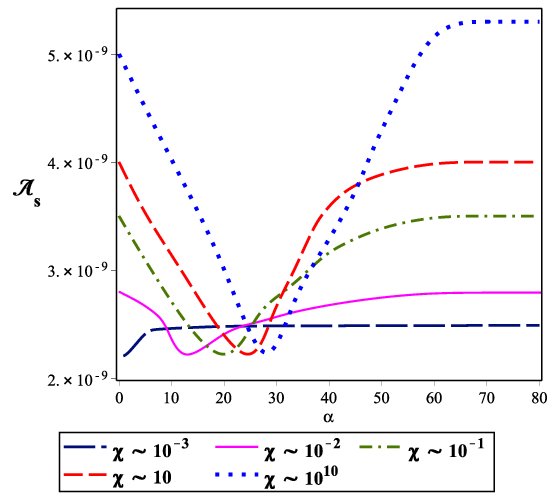
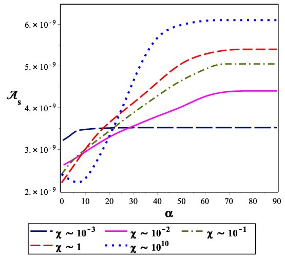
Figure 1: Power spectrum versus the free parameter $\alpha$ in a nonminimal derivative model in which the nonminimal coupling is a constant and the potential is E-model one. The left panel corresponds to $N=60$ and the right panel is for $N=70$.

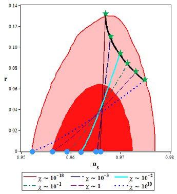
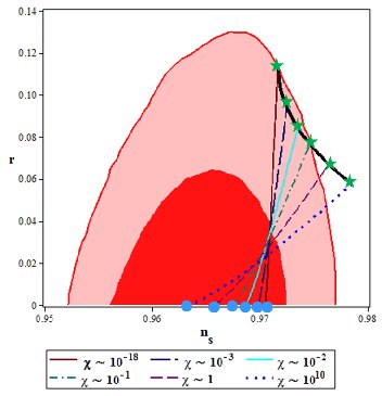
Figure 2: Tensor-to-scalar ratio versus the scalar spectral index in a nonminimal derivative model in which the nonminimal coupling is a constant and the potential is E-model one. The left panel corresponds to $N=60$ and the right panel is for $N=70$. The green stars show $\alpha\rightarrow\infty$ limit and the blue circles show $\alpha\rightarrow 0$ limit.

Table 1: Constraints on $\alpha$ by comparing the scalar spectral index and tensor-to-scalar ratio with Planck2015 TT, TE, EE+lowP data. These constraints are corresponding to a nonminimal derivative model in which the nonminimal coupling is a constant and the potential is E-model.

	$\chi\sim 10^{-3}$		$\chi\sim 10^{-2}$		$\chi\sim 10^{-1}$		$\chi\sim 1$		$\chi\sim 10^{18}$
$N=60\,,\,68\%$ CL	$\alpha<58$		$\alpha<61$		$\alpha<72$		$\alpha<76$		$\alpha<85$
$N=60\,,\,95\%$ CL	all values of $\alpha$		all values of $\alpha$		all values of $\alpha$		all values of $\alpha$		all values of $\alpha$
$N=70\,,\,68\%$ CL	$\alpha<25$		$\alpha<29$		$\alpha<37$		$\alpha<44$		$\alpha<49$
$N=70\,,\,95\%$ CL	all values of $\alpha$		all values of $\alpha$		all values of $\alpha$		$\alpha<102$		$\alpha<90$

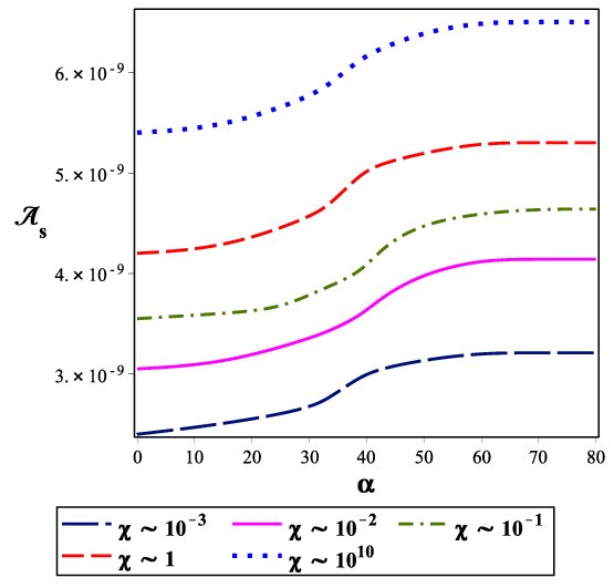
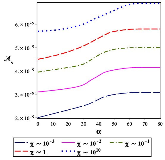
Figure 3: Power spectrum versus the free parameter $\alpha$ in a nonminimal derivative model in which both the nonminimal coupling and potential are E-model. The left panel corresponds to $N=60$ and the right panel is for $N=70$.

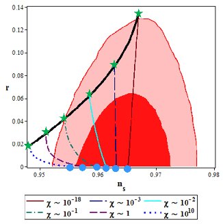
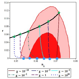
Figure 4: Tensor-to-scalar ratio versus the scalar spectral index in a nonminimal derivative model in which both the nonminimal coupling and potential are E-model. The left panel corresponds to $N=60$ and the right panel is for $N=70$. The green stars show $\alpha\rightarrow\infty$ limit and the blue circles show $\alpha\rightarrow 0$ limit.

Given these equations, now we can study the model numerically for both cases. By using $V$ and ${\cal{F}}$ defined as above, and solving the integral (16), we find the value of the field at the Hubble crossing in terms of the model’s parameters. By substituting $\phi_{hc}$ in equations (23), (24) and (31), we perform our numerical analysis. We define parameter $\chi$ as $\chi\equiv\frac{C}{M^{2}}$ which is dimensionless since $\lambda$ (and therefore $C$ from Eq. (38)) has the dimension of mass squared. We adopt several sample values of $\chi$ in our numerical analysis. Note that, two limits of NMDC model are the GR limit (corresponding to $\chi\rightarrow 0$) and high-friction limit (corresponding to $\chi\rightarrow\infty$). We take $\chi\sim 10^{-3}$, $\chi\sim 10^{-2}$, $\chi\sim 10^{-1}$, $\chi\sim 1$ and $\chi\sim 10^{10}$. The large value $\chi\sim 10^{10}$ is corresponding to the high-friction limit in NMDC model and it doesn’t violate the unitarity bound as we have explained in Introduction. By these adoption, we study the evolution of the power spectrum versus $\alpha$ for $N=60$ and $N=70$. The results are shown in figure 1. This figure corresponds to the functions defined in equations (33) and (35). Since from Planck2015 data the power spectrum is almost $2.4\times 10^{-9}$, it seems that considering E-model potential makes the power spectrum of the model to be viable. For instance, depending on the value of parameter $\chi$, the power spectrum takes the observed value with $10<\alpha<30$ for $N=60$. For the case with $N=70$, we can get ${\cal{A}}_{s}\sim 2.4\times 10^{-9}$ for $\chi<1$ and $\alpha<10$. However, in this case also the power spectrum is of the order of $10^{-9}$ for the adopted values of $\chi$. These situations are confirmed by exploring $r-n_{s}$ map. Figure 2 shows the tensor-to-scalar ratio versus the scalar spectral index for $N=60$ and $N=70$. Our analysis shows that by considering the E-model potential, it is possible to get $n_{s}=0.9652\pm 0.0047$ for all adopted values of $\chi$. For $N=70$, the scalar spectral index is equal to $0.9652\pm 0.0047$ only with $\chi>1$. However, the presence of the free parameter $\alpha$, causes $r-n_{s}$ plot with $N=70$ to lie in the background of the Planck2015 TT, TE, EE+lowP data, for all values of $\chi$ and in some ranges of $\alpha$. By comparing the values of the scalar spectral index and tensor-to-scalar ratio with $68\%$ and $95\%$ CL of Planck2015 TT, TE, EE+lowP data, we obtain some constraints on parameter $\alpha$ which are summarized in table 1. Note that, as figure 2 shows, in the NMDC model with E-model potential there is a critical line which the $r-n_{s}$ trajectories tend to. In $M\rightarrow\infty$ limit, we recover the attractor points in usual $\alpha$ attractor models (the line with $\chi\sim 10^{-18}$ shows almost this case), meaning that the presence of the line instead of point is because of considering the nonminimal derivatives coupling.

Table 2: Constraints on $\alpha$ by comparing the scalar spectral index and tensor-to-scalar ratio with Planck2015 TT, TE, EE+lowP data. These constraints are corresponding to a nonminimal derivative model in which both the nonminimal coupling and potential are E-model.

	$\chi\sim 10^{-3}$		$\chi\sim 10^{-2}$		$\chi\sim 10^{-1}$		$\chi\sim 1$		$\chi\sim 10^{18}$
$N=60\,,\,68\%$ CL	$\alpha<83$		$\alpha<78$		$\alpha<55$		$\alpha<9$		all values of $\alpha$
$N=60\,,\,95\%$ CL	all values of $\alpha$		all values of $\alpha$		all values of $\alpha$		$\alpha<46$		$\alpha<39$
$N=70\,,\,68\%$ CL	$\alpha<85$		$\alpha<80$		$\alpha<37$		$\alpha<7$		all values of $\alpha$
$N=70\,,\,95\%$ CL	all values of $\alpha$		all values of $\alpha$		all values of $\alpha$		$\alpha<38$		$\alpha<11$

We perform the same analysis for the NMDC model with functions defined in (33) and (37). The results are shown in figures 3 and 4. As these figures show, by adopting the E-model nonminimal derivative coupling function, the NMDC model would be observationally viable for all values of $\chi$ (even with large values such as $\chi\sim 10^{10}$). Whereas, NMDC model with $\phi^{2}$ potential is observationally viable just for some values of $\chi$. The power spectrum in this model is of the order of $10^{-9}$ (for $\chi\sim 10^{-3}$ it is possible to get ${\cal{A}}_{s}\sim 2.4\times 10^{-9}$) and $r-n_{s}$ plane lies in the background of Planck2015 TT, TE, EE+lowP data (for some ranges of parameter $\alpha$). In this case also, the $r-n_{s}$ trajectories tend to an attractor line in $\alpha\rightarrow 0$ limit. In the $M\rightarrow\infty$ limit we recover the attractor points as usual in $\alpha$-attractor models. By comparing the numerical results with $68\%$ and $95\%$ CL of Planck2015 TT, TE, EE+lowP data, we obtain some constraints on the free parameter $\alpha$ as shown in Table 2.

4 Nonlinear Perturbations and Non-Gaussianity

Regarding to the fact that by studying the two-point correlation function we are not able to get information about non-Gaussian feature of the primordial perturbations, then it is necessary to explore the three-point correlation function. To this end, we expand the action (9) up to the third order in the small perturbations. By introducing the new parameter ${\cal{X}}$ as follows

$${\cal{D}}=\frac{2(\kappa^{-2}+\frac{\dot{\phi}^{2}{\cal{F}}}{2M^{2}}){\Phi}}{2\kappa^{-2}H+3\frac{\dot{\phi}^{2}H{\cal{F}}}{M^{2}}}+\frac{a^{2}{\cal{X}}}{\kappa^{-2}+\frac{\dot{\phi}^{2}{\cal{F}}}{2M^{2}}}\,,\hskip 28.45274pt$$ (39)

and

$$\partial^{2}{\cal{X}}={\cal{W}}\dot{\Phi}\,,$$ (40)

we get the cubic action as

$$S_{3}=\int dt\,d^{3}x\,\Bigg{\{}\Bigg{[}\frac{3a^{3}}{\kappa^{2}c_{s}^{2}}\,\Bigg{(}1-\frac{1}{c_{s}^{2}}\Bigg{)}\epsilon\Bigg{]}{\Phi}\dot{\Phi}^{2}+\Bigg{[}\frac{a}{\kappa^{2}}\,\Bigg{(}\frac{1}{c_{s}^{2}}-1\Bigg{)}\epsilon\Bigg{]}{\Phi}\,(\partial{\Phi})^{2}$$

$$+\Bigg{[}\frac{a^{3}}{\kappa^{2}}\,\Bigg{(}\frac{1}{c_{s}^{2}\,H}\Bigg{)}\Bigg{(}\frac{1}{c_{s}^{2}}-1\Bigg{)}\epsilon\Bigg{]}\dot{\Phi}^{3}-\Bigg{[}a^{3}\,\frac{2}{c_{s}^{2}}\epsilon\dot{\Phi}(\partial_{i}{\Phi})(\partial_{i}{\cal{X}})\Bigg{]}\Bigg{\}}\,,$$ (41)

up to the leading order in the slow-roll parameters. The three point correlation function in the interaction picture is given by the following expression

$$\langle{\Phi}(\textbf{k}_{1})\,{\Phi}(\textbf{k}_{2})\,{\Phi}(\textbf{k}_{3})\rangle=(2\pi)^{3}\delta^{3}(\textbf{k}_{1}+\textbf{k}_{2}+\textbf{k}_{3}){\cal{B}}_{\Phi}(\textbf{k}_{1},\textbf{k}_{2},\textbf{k}_{3})\,,$$ (42)

where

$${\cal{B}}_{\Phi}(\textbf{k}_{1},\textbf{k}_{2},\textbf{k}_{3})=\frac{(2\pi)^{4}{\cal{A}}_{s}^{2}}{\prod_{i=1}^{3}k_{i}^{3}}\,{\cal{G}}_{\Phi}(\textbf{k}_{1},\textbf{k}_{2},\textbf{k}_{3}).$$ (43)

The parameter ${\cal{G}}_{\Phi}$ is given by

$${\cal{G}}_{\Phi}=\frac{3}{4}\Bigg{(}1-\frac{1}{c_{s}^{2}}\Bigg{)}\Bigg{(}\frac{2\sum_{i>j}k_{i}^{2}\,k_{j}^{2}}{k_{1}+k_{2}+k_{3}}-\frac{\sum_{i\neq j}k_{i}^{2}\,k_{j}^{3}}{(k_{1}+k_{2}+k_{3})^{2}}\Bigg{)}-\frac{1}{4}\Bigg{(}1-\frac{1}{c_{s}^{2}}\Bigg{)}\Bigg{(}\frac{2\sum_{i>j}k_{i}^{2}\,k_{j}^{2}}{k_{1}+k_{2}+k_{3}}$$

$$-\frac{\sum_{i\neq j}k_{i}^{2}\,k_{j}^{3}}{(k_{1}+k_{2}+k_{3})^{2}}+\frac{1}{2}\sum_{i}k_{i}^{3}\Bigg{)}+\frac{3}{2}\Bigg{(}\frac{1}{c_{s}^{2}}-1\Bigg{)}\Bigg{(}\frac{\left(k_{1}\,k_{2}\,k_{3}\right)^{2}}{(k_{1}+k_{2}+k_{3})^{3}}\Bigg{)}.$$ (44)

One can use this parameter to define the so-called “nonlinearity parameter” as

$$f_{NL}=\frac{10}{3}\frac{{\cal{G}}_{\Phi}}{\sum_{i=1}^{3}k_{i}^{3}}\,,$$ (45)

which measures the amplitude of the non-Gaussianity of the perturbations. By adopting different values of the three momenta $k_{1}$ , $k_{2}$ and $k_{3}$, we can get different shapes of the non-Gaussianity (see for instance [55, 56, 57, 58]). In some inflation models (we can refer, for instance, the DBI, k-inflation and higher derivative models) the non-Gaussianity is constructed at horizon crossing during inflation epoch. In such models, when all three wavelengths are equal to the size of the horizon, there would be a maximal signal in the bispectrum [59, 60]. In these models, it is useful to study the “equilateral” configuration of the non-Gaussianity. In this setup and in the equilateral configuration we have

$${\cal{G}}_{\Phi}^{equil}=\frac{17}{72}k^{3}\left(1-\frac{1}{c_{s}^{2}}\right)\,,$$ (46)

leading to

$$f_{NL}^{equil}=\frac{85}{324}\left(1-\frac{1}{c_{s}^{2}}\right)\,.$$ (47)

Now, we can analyze the model numerically. From equation (47) we see that the equilateral amplitude of the non-Gaussianity corresponds to the sound speed. On the other hand, the sound speed is related to the tensor-to-scalar ratio via equation (31). The evolution of the sound speed versus the tensor-to-scalar ratio for models given by equations (35) and (37) are shown in figures 5 and 6 respectively. Given that the tensor-to-scalar ratio is constrained by using the $95\%$ CL of Planck2015 TT, TE, EE+lowP data, we can find some constraints on the sound speed in this model. The constrained are summarized in tables 3 and 4. As regard to the admissible values of $r$, it is possible to have small sound speed. Since the amplitude of the equilateral configuration of the non-Gaussianity is related to the sound speed via equation (47), with the small sound speed it is possible to have large amplitude of the non-Gaussianity. In figures 7 and 8 we have plotted the equilateral configuration of the non-Gaussianity versus the sound speed for some sample values of $\chi$ in the background of Planck2015 TTT, EEE, TTE and EET data. Figure 7 corresponds to the function defined in equation (35) and figure 8 is corresponding to the one defined in equation (37). As we see, in some ranges of the model’s parameter, the amplitude of the non-Gaussianity in NMDC $\alpha$-attractor model is consistent with Planck2015 TTT, EEE, TTE and EET data.

Table 3: Constraints on the sound speed and tensor-to-scalar ratio obtained from $95\%$ CL of Planck2015 TT, TE, EE+lowP data. These constraints are corresponding to a nonminimal derivative model in which the nonminimal coupling is a constant and the potential is E-model.

	$\chi\sim 10^{-3}$		$\chi\sim 10^{-2}$		$\chi\sim 10^{-1}$		$\chi\sim 1$		$\chi\sim 10^{18}$
$N=60\,\,$	$r<0.108$		$r<0.092$		$r<0.083$		$r<0.074$		$r<0.066$
$N=60\,\,$	$c_{s}^{2}<0.622$		$c_{s}^{2}<0.527$		$c_{s}^{2}<0.457$		$c_{s}^{2}<0.389$		$c_{s}^{2}<0.328$
$N=70\,\,$	$r<0.092$		$r<0.082$		$r<0.075$		$r<0.06$		$r<0.046$
$N=70\,\,$	$c_{s}^{2}<0.511$		$c_{s}^{2}<0.448$		$c_{s}^{2}<0.391$		$c_{s}^{2}<0.309$		$c_{s}^{2}<0.244$

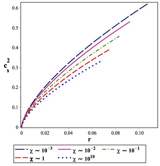
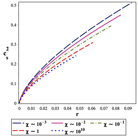
Figure 5: Sound speed versus the tensor-to-scalar ratio in a nonminimal derivative model in which the nonminimal coupling is a constant and the potential is E-model. The left panel corresponds to $N=60$ and the right panel is for $N=70$.

Table 4: Constraints on the sound speed and tensor-to-scalar ratio obtained from $95\%$ CL of Planck2015 TT, TE, EE+lowP data. These constraints are corresponding to a nonminimal derivative model in which both the nonminimal coupling and potential are E-model.

	$\chi\sim 10^{-3}$		$\chi\sim 10^{-2}$		$\chi\sim 10^{-1}$		$\chi\sim 1$		$\chi\sim 10^{18}$
$N=60\,\,$	$r<0.088$		$r<0.061$		$r<0.039$		$r<0.029$		$r<0.018$
$N=60\,\,$	$c_{s}^{2}<0.422$		$c_{s}^{2}<0.312$		$c_{s}^{2}<0.213$		$c_{s}^{2}<0.16$		$c_{s}^{2}<0.105$
$N=70\,\,$	$r<0.091$		$r<0.080$		$r<0.065$		$r<0.059$		$r<0.055$
$N=70\,\,$	$c_{s}^{2}<0.514$		$c_{s}^{2}<0.444$		$c_{s}^{2}<0.365$		$c_{s}^{2}<0.324$		$c_{s}^{2}<0.292$

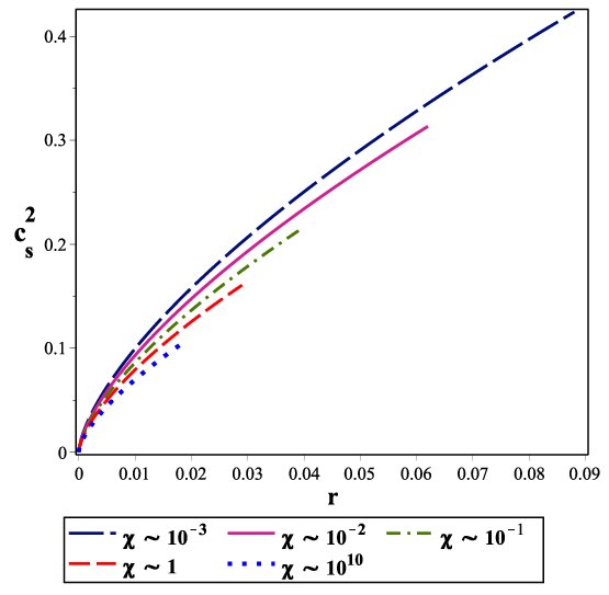
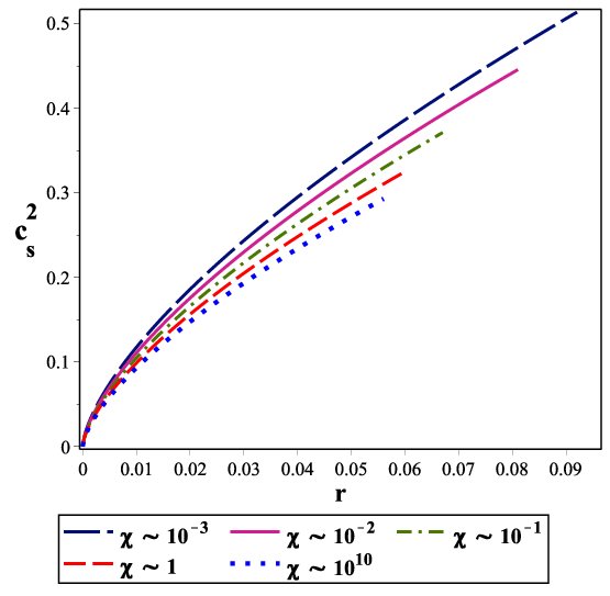
Figure 6: Sound speed versus the tensor-to-scalar ratio in a nonminimal derivative model in which both the nonminimal coupling and potential are E-model. The left panel corresponds to $N=60$ and the right panel is for $N=70$.

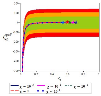
Figure 7: Amplitude of the equilateral configuration of the non-Gaussianity versus the sound speed in a nonminimal derivative model in which the nonminimal coupling is a constant and the potential is E-model. The left panel corresponds to $N=60$ and the right panel is for $N=70$. Note that, here the stars show the maximum values of the sound speed in each case.

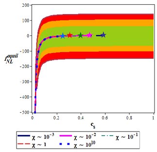
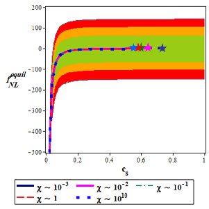
Figure 8: Amplitude of the equilateral configuration of the non-Gaussianity versus the sound speed in a nonminimal derivative model in which both the nonminimal coupling and potential are E-model. The left panel corresponds to $N=60$ and the right panel is for $N=70$. The stars show the maximum values of the sound speed in each case.

5 Summary

The aim of this paper was to study the non-minimal derivative model in the context of $\alpha$-attractor. In this regard, we have considered a two-fields action in which both the fields and their derivatives are nonminimally coupled to the gravity. We have used the conformal gauge to convert the two-fields model into a one field which its derivative (and not the field itself) is nonminimally coupled to the gravity. After obtaining the the background equations of this NMDC model, we have studied the linear perturbations theory. By adopting the ADM formalism, we have studied both the scalar and tensor perturbations in this setup and found some important perturbation parameters like as the power spectrum, scalar spectral index and tensor-to-scalar ratio. After that, by introducing the types of the general functions $\hat{{\cal{F}}}(\psi,\varphi)$ and $U(\psi,\varphi)$, and using the conformal gauge, the NMDC function and potential have been obtained. In this paper, two types of NMDC function have been considered; ${\cal{F}}=const.$ and ${\cal{F}}={\cal{F}}(\phi)$. We have shown that in both cases there is an attractor line in large $N$ and small $\alpha$ limits which the $r-n_{s}$ trajectories tend to, while in the the single field $\alpha$-attractor model there is an attractor point in these limits. In fact, the presence of attractor line instead of attractor point is due to the nonminimal derivatives coupling that causes the scalar spectral index of this model to be a functions of two parameters, $\alpha$ and $M$. In the limit $M\rightarrow\infty$, one recovers the attractor point as is usual in $\alpha$-attractor models. We have numerically studied the linear perturbation in two cases with constant NMDC coupling and E-model NMDC coupling (in both cases the potential is considered to be E-model). With these choices, the power spectrum of the perturbations in NMDC model can get the observationally viable value (almost $2.4\times 10^{-9}$) in some ranges of $\chi$ and $\alpha$. Also, in this model $r-n_{s}$ plane lies in the background of Planck2015 TT, TE, EE+lowP data for all values of $M$ (or $\chi$) and in some ranges of $\alpha$, for both $N=60$ and $N=70$. We have obtained some constraints on the free parameter $\alpha$ which lead to the values of the scalar spectral index and tensor-to-scalar ratio which are consistent with $68\%$ and $95\%$ CL of the Planck2015 TT, TE, EE+lowP data for $r-n_{s}$ distribution. By studying the nonlinear perturbation and three point correlation functions, we have studied the non-Gaussian feature of the primordial perturbations. In this regard we have obtained the amplitude of the equilateral configuration of the non-Gaussianity in terms of the sound speed. The sound speed is related to the tensor-to-scalar ratio via the consistency relation. The tensor-to-scalar ratio is constrained by using the $95\%$ CL of the Planck2015 TT, TE, EE+lowP data for $r-n_{s}$ distribution. By using the constraints on the tensor-to-scalar ratio, we have obtained some constraints on the values of the sound speed in this model. In this regard, we have shown that it is possible to have small sound speed leading to the large non-Gaussianity in this NMDC $\alpha$-attractor model.

Acknowledgement
We would like to appreciate the referee for very insightful comments that have boosted the quality of the paper considerably. This work has been supported financially by Research Institute for Astronomy and Astrophysics of Maragha (RIAAM) under research project number 1/5237-97.

References

- [1] A. Guth, Phys. Rev. D 23, 347 (1981).
- [2] A. D. Linde, Phys. Lett. B 108, 389 (1982).
- [3] A. Albrecht and P. Steinhard, Phys. Rev. D 48, 1220 (1982).
- [4] A. D. Linde, Particle Physics and Inflationary Cosmology (Harwood Academic Publishers, Chur, Switzerland, 1990). [arXiv:hep-th/0503203].
- [5] A. Liddle and D. Lyth, Cosmological Inflation and Large-Scale Structure, (Cambridge University Press, 2000).
- [6] J. E. Lidsey et al, Abney, Rev. Mod. Phys. 69, 373 (1997).
- [7] A. Riotto, [arXiv:hep-ph/0210162].
- [8] D. H. Lyth and A. R. Liddle, The Primordial Density Perturbation (Cambridge University Press, 2009).
- [9] J. M. Maldacena, JHEP 0305, 013 (2003).
- [10] N. Bartolo, E. Komatsu, S. Matarrese and A. Riotto, Phys. Rept. 402, 103 (2004).
- [11] X. Chen, Adv. Astron. 2010, 638979 (2010).
- [12] Q.-G. Huang and Yi Wang, JCAP 06,035 (2013).
- [13] A. De Felice and S. Tsujikawa, Phys. Rev. D 84, 083504 (2011).
- [14] A. De Felice and S. Tsujikawa, JCAP 1104, 029 (2011).
- [15] K. Nozari and N. Rashidi, Phys. Rev. D 86, 043505 (2012).
- [16] K. Nozari and N. Rashidi, Phys. Rev. D 88, 023519 (2013).
- [17] K. Nozari and N. Rashidi, Phys. Rev. D 88, 084040 (2013).
- [18] K. Nozari and N. Rashidi, Astrophys. Space Sci. 350, 339 (2014).
- [19] L. Amendola, Phys. Lett. B 301, 175 (1993).
- [20] C. Germani and A. Kehagias, Phys. Rev. Lett. 105, 011302 (2010).
- [21] C. Germani, Phys. Rev. D 86, 104032 (2012).
- [22] C. Germani, Rom. J. Phys. 57, 841 (2012).
- [23] S. Tsujikawa, Phys. Rev. D 85, 083518 (2012).
- [24] E. N. Saridakis and S. V. Sushkov, Phys. Rev. D 81, 083510 (2010).
- [25] K. Nozari and N. Rashidi, Phys. Rev. D 93, 124022 (2016).
- [26] K. Nozari and N. Rashidi, Advances in High Energy Physics 2016, 1252689 (2016).
- [27] R. Kallosh and A. Linde, JCAP 1307, 002 (2013).
- [28] R. Kallosh and A. Linde, JCAP 1312, 006 (2013).
- [29] D. I. Kaiser and E. I. Sfakianakis, Phys. Rev. Lett. 112, 011302 (2014).
- [30] S. Ferrara, R. Kallosh, A. Linde and M. Porrati, Phys. Rev. D 88, 085038 (2013).
- [31] R. Kallosh, A. Linde and D. Roest, JHEP 1311, 198 (2013).
- [32] R. Kallosh, A. Linde and D. Roest, JHEP 1408, 052 (2014).
- [33] S. Cecotti and R. Kallosh, JHEP 05, 114 (2014).
- [34] R. Kallosh and A. Linde, JCAP 1306, 028 (2013).
- [35] R. Kallosh, A. Linde and D. Roest, JHEP 09, 062 (2014).
- [36] A. Linde, JCAP 05, 003 (2015).
- [37] J. Joseph, M. Carrasco, R. Kallosh and A. Linde, Phys. Rev. D 92, 063519 (2015).
- [38] J. Joseph, M. Carrasco, R. Kallosh and A. Linde, JHEP 10, 147 (2015).
- [39] R. Kallosh, A. Linde, D. Roest and T. Wrase, JCAP 1611, 046 (2016).
- [40] M. Shahalam, R. Myrzakulov, S. Myrzakul and A. Wang, [arXiv:1611.06315 [astro-ph.CO]].
- [41] S. D. Odintsov and V. K. Oikonomou, Phys. Rev. D 94, 124026 (2016).
- [42] N. Rashidi and K. Nozari, Int. J. Mod. Phys. D 27, 1850076 (2018).
- [43] E. Komatsu et al. [WMAP Collaboration], Astrophys. J. Suppl. 192, 18 (2011).
- [44] W. Percival et al., Mon. Not. R. Astron. Soc. 401, 2148 (2010).
- [45] A. G. Riess et al., Astrophys. J. 699, 539 (2009).
- [46] P. A. R. Ade et al., [arXiv:1502.02114] [astro-ph.CO].
- [47] A. A. Starobinsky, Phys. Lett. B 91, 99 (1980).
- [48] A. A. Starobinsky, Sov. Astron. Lett. 9, 302 (1983).
- [49] B. Whitt, Phys. Lett. B 145, 176 (1984).
- [50] K. Nozari and N. Rashidi, Phys. Rev. D 95, 123518 (2017).
- [51] D. Bettoni and S. Liberati, Phys. Rev. D 88, 084020 (2013).
- [52] V. F. Mukhanov, H. A. Feldman, R. H. Brandenberger, Phys. Rept. 215, 203, (1992).
- [53] D. Baumann, [arXiv:0907.5424][hep-th].
- [54] M. P. Hertzberg, Phys. Lett. B 745, 118 (2015).
- [55] L. Wang and M. Kamionkowski, Phys. Rev. D 61, 063504 (2000).
- [56] E. Komatsu and D. N. Spergel, Phys. Rev. D 63, 063002 (2001).
- [57] D. Babich, P. Creminelli and M. Zaldarriaga, J. Cosmology Astropart. Phys. 8, 9 (2004).
- [58] L. Senatore, K. M. Smith and M. Zaldarriaga, J. Cosmology Astropart. Phys. 1, 28 (2010).
- [59] D. Babich, P. Creminelli and M. Zaldarriaga, JCAP 0408, 009 (2004).
- [60] P. Creminelli, A. Nicolis, L. Senatore, M. Tegmark and M. Zaldarriaga, JCAP 0605, 004 (2006).