Generalized Four Moment Theorem and an Application to CLT for Spiked Eigenvalues of high-dimensional Covariance Matrices.

Abstract

We consider a more generalized spiked covariance matrix $\Sigma$, which is a general non-definite matrix with the spiked eigenvalues scattered into a few bulks and the largest ones allowed to tend to infinity. By relaxing the matching of the 4th moment to a tail probability decay, a Generalized Four Moment Theorem (G4MT) is proposed to show the universality of the asymptotic law for the local spectral statistics of generalized spiked covariance matrices, which implies the limiting distribution of the spiked eigenvalues of the generalized spiked covariance matrix is independent of the actual distributions of the samples satisfying our relaxed assumptions. Moreover, by applying it to the Central Limit Theorem (CLT) for the spiked eigenvalues of the generalized spiked covariance matrix, we remove the strict constraint of diagonal block independence for the population covariance matrix given in Bai and Yao (2012), and extend their result to a general case that the 4th moment and the spiked eigenvalues are not necessarily required to be bounded and the population covariance matrix is in a general form, thus meeting the actual cases better.

arXiv:0000.0000

and

t1Corresponding author; Supported by Project 11471140 from NSFC. t2Supported by Project 11571067 from NSFC.

1 Introduction

The study on the universality conjecture for the local spectral statistics of random matrices, which is motivated by similar phenomena in physics, has been one of the key topics in random matrix theory. It not only plays an important role in the local field of statistics, but has also been widely used in many other fields, such as mathematical physics, combinatorics and computing science. In this paper, we are going to propose a Generalized Four Moment Theorem (G4MT) to prove the universality of the asymptotic law for the local spiked eigenvalues of generalized spiked covariance matrices, and then apply it to the Central Limit Theorem (CLT) for the spiked eigenvalues of the generalized spiked covariance matrix in a general case.

1.1 Background of universality

As is well known, universality has been conjectured by many statisticians since the 1960s, including Wigner (1958), Dyson (1970), and Mehta (1967); it states that local statistics are universal, implying that the conclusions hold not only for the Gaussian Unitary Ensemble (GUE) but also the general Wigner random matrix. It provides new ideas and techniques for the research of random matrix theory, which implies that to prove one result suitable for Non-Gaussian case, it is sufficient to show the same result under the Gaussian assumption if the universality is true.

The similar universality phenomena of the bulk of the spectrum has been also investigated in many studies. A rigorous result has emerged in Soshnikov (1999), which proved that the universality of the joint distribution of the largest $k$ eigenvalues (for any fixed $k$) hold under the symmetric assumption of the atom distribution. Johansson (2001), Ben and Péché (2005) focused on the Gauss divisible, which is a strong regularity assumption on the atom distribution. Further, Erdős, et al. (2010a) relaxed the above regularity assumption to a distribution family with a explicit form. Erdős, et al. (2010b) improved the work by the analysis of the Dyson Brownian motion but still requires a high degree of regularity on the atom distribution. Most recently, Tao and Vu (2015) showed the universality of the asymptotic law for the local spectral statistics of the Wigner matrix by the Four Moment Theorem, which is based on the Lindeberg strategy in Lindeberg (1922) of replacing non-Gaussian random variables with Gaussian ones. This method assumes that the moments of the entries match that of the complex standardized Gaussian ensemble up to the 4th order and requires the $C_{0}$ condition to hold, which states that the independent distributed entries have zero mean and identity variance and satisfy the uniform exponential decay, with the form

$$P(|x_{ij}|\geq t^{C})\leq e^{-t}$$

for all $t\geq C^{\prime}$, $1\leq i,j\leq n$ and $C,C^{\prime}$ being some constants. Although they asserted that the fine spacing statistics of a random Hermitian matrix in the bulk of the spectrum are only sensitive to the first four moments of the entries, they also conjectured that it may be possible to reduce the number of matching moments in their theorem.

1.2 Our contribution to universality

Inspired by these previous works, the G4MT is proposed by replacing the condition of matching the 4th moment by a tail probability as detailed in Assumption ${\bf B}$. Then the universality of the asymptotic law for the bulk of spiked eigenvalues of generalized covariance matrices is automatically proved by the proposed G4MT. By weakening the constrains, it takes several advantages as follows: First, when proving the universality of the asymptotic law for the bulk of the spiked eigenvalues, It only requires the condition of matching moments up to the 3th order and the fourth moments to satisfy the tail probability, which is a regular and necessary condition in the weak convergence of the largest eigenvalue. For the case of symmetric distribution, it is only needed to consider the first and the second moments. Second, we reduce the study of universality of a asymptotic law to the eigenvalues of a low-dimensional matrix, unlike Tao and Vu (2015) which involves the partial derivative operation of the whole large dimensional random matrices. As a by-product, the rigorous $C_{0}$ condition having uniform exponential decay in Tao and Vu (2015) is also not necessary. Finally, it shows that the limiting distribution of the spiked eigenvalues of a generalized spiked covariance matrix is independent of the actual distributions of the samples satisfying our relaxed assumptions.

As an application, we also apply the proposed G4MT to the CLT for the spiked eigenvalues of the generalized spiked covariance matrix. By relaxing the constrains, we remove some of the strict conditions given in Bai and Yao (2012), and then make the result efficient in a wider usage, where the 4th moment and the spiked eigenvalues are not necessarily required to be bounded and the population covariance matrix is in a general form without diagonal block independent assumption, thus meeting the actual cases better.

1.3 Related works of spiked model

The spiked model in the high-dimensional setting is originated from the common phenomenon of large or even huge dimensionality $p$ compared to the sample size $n$, occurring in many modern scientific fields, such as wireless communication, gene expression and climate studies. It was first proposed by Johnstone (2001) under the assumptions of high dimensionality and an identity population covariance matrix with fixed and relatively small spikes. Since the study of spiked covariance matrices has a close relationship with Principal Component Analysis (PCA) or Factor Analysis (FA), which are important and powerful tools in dimension reduction, data visualization and feature extraction, it has inspired great interest on the part of researchers in the limiting behaviors of the eigenvalues and eigenvectors of such high-dimensional spiked sample covariance.

Within this context, many impressive works are devoted to investigate on the limiting properties of the spiked eigenvalues of the high-dimensional covariance matrix. The initial focus was on the simplest situation that the population covariance matrix is a small perturbation of the identity covariance matrix. Under this simplified assumption, Baik, et al. (2005) investigated the exact scaling rates of the asymptotic distributions of the empirical eigenvalues in both cases of below and above the related threshold. Baik and Silverstein (2006) provided the almost sure limits of the sample eigenvalues in the simplified spiked model for a general class of samples when both population size and sample size tend to infinity with a finite ratio. Paul (2007) showed the asymptotic structure of the sample eigenvalues and eigenvectors with bounded spikes in the setting of $p/n\rightarrow c_{0}\in(0,1)$ as $n\rightarrow\infty$. Bai and Yao (2008) derived the phase transition and the CLT of the spiked eigenvalues when the entries of the samples are independent and identically distributed (${\rm i.i.d.}$).

To improve the simplified assumptions, Bai and Yao (2012) contributed to deal with a more general spiked covariance matrix, which assumed the conditions of the diagonal block independence and finite 4th moments. Efforts have also been devoted to PCA or FA as a different way to improve the work on the spiked population model. For example, Bai and Ng (2002) focused on the determination of the number of factors and first established the convergence rate for the factor estimates with the constrains of the independence of the components and the existence of the 8th moment. Hoyle and Rattray (2004) used the replica method to evaluate the expected eigenvalue distribution as the $p/n\to c$, a fixed constant. The work is considered in the case of a number of symmetry-breaking directions. Onatski (2009) derived accurate approximations to the finite sample distribution of the principal components estimator in the large factor model with weakly influential factors. The more general works are the recent contributions from Wang and Fan (2017) and Cai, et al. (2019) , which both investigate the asymptotic distributions of the spiked eigenvalues and eigenvectors of a general covariance matrix. However, the result of Wang and Fan (2017) only has one threshold, which is the same as the case of block independence indeed. More importantly, their main theorems are involved with the difference between the ratio $\lambda_{i}/\alpha_{i}$ and 1, with $\lambda_{i}$ being the corresponding sample eigenvalue, which is given as an unspecified ”O” term. Furthermore, both of the works in Wang and Fan (2017) and Cai, et al. (2019) require the bounded 4th moments and the condition $p/(n\alpha_{i})\to 0$, with $\alpha_{i},i=1,\cdots,K$ being the spikes, so that it limits the relationship between the dimensionality and the spikes.

On the basis of these works, we further consider a general spiked covariance matrix and study the asymptotic law for its spiked eigenvalues under relaxed assumptions. Since the main cause of this unspecified ”O” term is the use of the population spiked eigenvalue in the ratio $\lambda_{i}/\alpha_{i}$, but not its phase transition, so that we consider to use the phase transition of the spiked eigenvalues instead and then give the explicit CLT for the spiked eigenvalues of high-dimensional generalized covariance matrices.

1.4 Our contribution to spiked model

To improve the related works on spiked model, we shall apply the proposed G4MT to the CLT for the spiked eigenvalues of the generalized spiked covariance matrix as mentioned in Sec 1.2. We consider a general spiked covariance matrix $\Sigma$, which is a general non-definite matrix with the spectrum formed as

$$\beta_{p,1},\cdots,\beta_{p,j},\cdots,\beta_{p,p}$$ (1.1)

in descending order and $\beta_{p,j_{k}+1},\cdots\beta_{p,j_{k}+m_{k}}$ are equal to $\alpha_{k},k=1,\cdots,K$, respectively, where $j_{k}$ is the rank of the eigenvalue in front of the first $\alpha_{k}$ in the array (1.1) and $j_{k}$ also may take value at 0. Then, $\alpha_{1},\cdots,\alpha_{K}$ with multiplicity $m_{k},k=1,\cdots,K$, respectively, satisfying $m_{1}+\cdots+m_{K}=M$, a fixed integer, are the spiked eigenvalues of $\Sigma$ lined arbitrarily in groups among all the eigenvalues. We apply the G4MT to the spiked eigenvalues of such general covariance matrix $\Sigma$, and provide a universal asymptotic distribution of the spiked eigenvalues of the generalized spiked covariance matrix. By our relaxing constraints, the proposed result demonstrates several advantages as below: First, we remove the strict condition that the population covariance matrix has a diagonal block independent structure given in Bai and Yao (2012). As known, their diagonal block structure is equivalent to require that the spiked and non-spiked eigenvalues are generated from the independent variables, which is difficult to reach for the huge data today. Second, our method permits the spiked eigenvalues to be scattered into a few bulks, any of which are larger than their related right-threshold or smaller than their related left-threshold. So our focused work is extended to a generalized case with a few pairs of thresholds. Furthermore, for the generalized population covariance matrix that satisfies the Assumption D, we give a clear and universal expression for the limit distribution of the spiked eigenvalues of generalized spiked covariance matrix, which is not involved with an unspecified ”O” term and the 4th moments. For the cases that the Assumption D is not met, such as the diagonal matrix or the diagonal block matrix, we also provide the corresponding result in Remark 3.1, which performs as well as the approach in Bai and Yao (2012), and even better in some cases as illustrated in simulations. Finally, the spiked eigenvalues and the population 4th moments are not necessarily required to be bounded in our work. Thus the weakening constraints make the conclusion more applicable to actual cases.

The rest of our paper is arranged as follows: In Section 2, the problem is described in a generalized setting, and the phase transition for the spiked eigenvalues of generalized covariance matrix is also presented. Section 3 gives the main results of the G4MT and applies it to the CLT for the spiked eigenvalues of the generalized spiked covariance matrix in high-dimensional setting. In Section 4, simulations are conducted to evaluate our work comparing with the work in Bai and Yao(2012). Then, an applications to determining the number of the spikes and real data analysis are also discussed in Section 5. Finally, we draw a conclusion in the Section 6. Important proofs are all provided in the Supplement.

2 Problem Description and Preliminaries

Consider the random samples $T_{p}{\bf X}$, where

$${\bf X}=({\bf x}_{1},\cdots,{\bf x}_{n})=\left(x_{ij}\right),1\leq i\leq p,~{}1\leq j\leq n,$$

and $T_{p}$ is a $p\times p$ deterministic matrix. Then, $T_{p}T_{p}^{*}=\Sigma$ is the population covariance matrix, which can be seen as a general non-definite matrix with the spectrum arranged in descending order in (1.1). The population spiked eigenvalues of $\Sigma$, $\alpha_{1},\cdots,\alpha_{K}$ with multiplicities $m_{k},k=1,\cdots,K$, are lined arbitrarily in groups among all the eigenvalues, where $m_{1}+\cdots+m_{K}=M$ is a fixed integer.

Define the corresponding sample covariance matrix of the observations $T_{p}{\bf X}$ as

$$S=T_{p}\left(\frac{1}{n}{\bf X}{\bf X}^{*}\right)T_{p}^{*},$$ (2.1)

and then the sample covariance matrix $S$ is the so-called generalized spiked sample covariance matrix.

Define the singular value decomposition of $T_{p}$ as

$$T_{p}=V\left(\begin{array}[]{cc}D_{1}^{1/2}&{\bf 0}\\ {\bf 0}&D_{2}^{1/2}\end{array}\right)U^{*},$$ (2.2)

where $U$ and $V$ are unitary matrices, $D_{1}$ is a diagonal matrix of the $M$ spiked eigenvalues and $D_{2}$ is the diagonal matrix of the non-spiked eigenvalues with bounded components. Since the investigation on the limiting distribution of the spiked eigenvalues of the sample covariance matrix depends on the basic equation $|\lambda{\bf I}-S|=0$, it is obvious that it only involves the right singular vector matrix $U$ but not the left one.

Let $J_{k}$ be the set of ranks of $\alpha_{k}$ with multiplicity $m_{k}$ among all the eigenvalues of $\Sigma$, i.e.

$$J_{k}=\{j_{k}+1,\cdots,j_{k}+m_{k}\}.$$

Denote by $\{l_{j}({\bf A})\}$ the eigenvalues of a $p\times p$ matrix ${\bf A}$. Then, the sample eigenvalues of the generalized spiked sample covariance matrix $S$ are sorted in descending order as

$$l_{1}(S),\cdots,l_{j}(S),\cdots,l_{p}(S).$$

To consider the limiting distribution of the spiked eigenvalues of a generalized sample covariance matrix $S$, it is necessary to determine the following assumptions:

Assumption [A​​

] The double array $\{x_{ij},i,j=1,2,...\}$ consist of ${\rm i.i.d.}$ random variables with mean 0 and variance 1. Furthermore, ${\rm E}x_{ij}^{2}=0$ for the complex case (when both $x$’s and $T_{p}$ are complex).

Assumption [B​​

] Suppose that

$$\lim\limits_{\tau\rightarrow\infty}\tau^{4}{\rm P}\left(|x_{ij}|>\tau\right)=0$$

for the i.i.d. sample $(x_{i1},\cdots,x_{in}),$ $i=1,\cdots,p$, where the 4th moments may unnecessarily exist.

Assumption [C​​

] The $p\times p$ matrix $\Sigma=T_{p}T_{p}^{*}$ forms the sequence $\{\Sigma_{p}\}$, which is bounded in the spectral norm. Moreover, denote the empirical spectral distribution (ESD) of $\Sigma$ as $H_{n}$, which tends to a proper probability measure $H$ as $p\rightarrow\infty$.

Assumption [D​​

] Suppose that

$$\max\limits_{t,s}|u_{ts}|^{2}\left({{\rm E}|x_{11}|^{4}-3}\right)I(|x_{11}|<\sqrt{n})\rightarrow 0,$$ (2.3)

where $U_{1}=\big{(}u_{ts}\big{)}_{t=1,\cdots,p;s=1,\cdots,M}$ is the first $M$ columns of matrix $U$ defined in (2.2).

The detailed explanation of Assumption D can be found in the Supplementary materials.

Assumption [E​​

] Assuming that $p/n=c_{n}\to c>0$ and both $n$ and $p$ go to infinity simultaneously, the spiked eigenvalues of the matrix $\Sigma$, $\alpha_{1},\cdots,\alpha_{K}$ with multiplicities $m_{1},\cdots,m_{K}$ laying out side the support of $H$, satisfy $\phi^{\prime}(\alpha_{k})>0$ for $1\leq k\leq K$, where

$$\phi(x)=x\left(1+c\int\frac{t}{x-t}\mbox{d}H(t)\right)$$

is detailed in the following Proposition 2.1.

2.1 Phase transition of the spiked eigenvalues of generalized covariance matrices.

In this part, an improved version of the phase transition for each spiked eigenvalue of a generalized sample covariance matrix is detailed under our relaxed assumptions. For each population spiked eigenvalue $\alpha_{k}$ with multiplicity $m_{k}$ and the associated sample eigenvalues $\{l_{j}(S),j\in J_{k}\}$, $k=1,\cdots,K$, we have following proposition

Proposition 2.1.

For the spiked sample covariance matrix $S$ given in (2.1), assume that $p/n=c_{n}\to c>0$ and both the dimensionality $p$ and the sample size $n$ grow to infinity simultaneously. For any population spiked eigenvalue $\alpha_{k},(k=1,\cdots,K)$, let

$$\rho_{k}=\left\{\begin{array}[]{cc}\phi(\alpha_{k}),&\mbox{ if }\phi^{\prime}(\alpha_{k})>0,\\ \phi(\underline{\alpha}_{k}),&\mbox{ if there exists }\underline{\alpha}_{k}\mbox{ such that }\phi^{\prime}(\underline{\alpha}_{k})=0\\ &\mbox{ and }\phi_{n}^{\prime}(t)<0,\mbox{ for all }\alpha_{k}\leq t<\underline{\alpha}_{k}\\ \phi(\overline{\alpha}_{k}),&\mbox{ if there exists }\overline{\alpha}_{k}\mbox{ such that }\phi^{\prime}(\overline{\alpha}_{k})=0\\ &\mbox{ and }\phi^{\prime}(s)<0,\mbox{ for all }\overline{\alpha}_{k}<s\leq\alpha_{k}\end{array}\right.$$

where

$$\phi(\alpha_{k})=\alpha_{k}\left(1+c\int\frac{t}{\alpha_{k}-t}\mbox{d}H(t)\right).$$ (2.4)

Then, it holds that for all $j\in J_{k}$, $\{{l_{j}}/{\rho_{k}}-1\}$ almost surely converges to 0.

Remark 2.1.

Since the convergence of $c_{n}\to c$ and $H_{n}\to H$ may be very slow, the difference $\sqrt{n}(l_{j}-\phi_{k})$ may not have a limiting distribution. Furthermore, from a view of statistical inference, $H_{n}$ can be treated as the subject population, and $c_{n}$ can be regarded as the ratio of dimension to sample size for the subject sample. So, we usually use

$$\phi_{n}(\alpha_{k})=\alpha_{k}\left(1+c_{n}\int\frac{t}{\alpha_{k}-t}\mbox{d}H_{n}(t)\right),$$ (2.5)

instead of $\phi_{k}$ in $\rho_{k}$, in particular during the process of CLT. Then, we only require $c_{n}=p/n$, and both the dimensionality $p$ and the sample size $n$ grow to infinity simultaneously, but not necessarily in proportion. Moreover, the approximation that $\{{l_{j}}/{\rho_{k}}-1\}$ almost surely converges to 0 still holds for all $j\in J_{k}$.

Note that the Proposition 2.1 theoretically shows that the diagonal block independent assumption of Bai and Yao (2012) can be removed, and both of the spiked eigenvalues and the population 4th moment are not necessarily required to be bounded. The proof of Proposition 2.1 can be easily obtained based on the G4MT, which is presented in the next section and shows that two samples, ${\bf X}$ and ${\bf Y}$, from different populations satisfying Assumptions ${\bf A}\sim{\bf E}$ will lead to the same limiting distribution of the spiked eigenvalues of a generalized spiked covariance matrix. By the G4MT, it is reasonable to assume the Gaussian entries from ${\bf X}$; then, Proposition 2.1 is proved by the almost sure convergence and the exact separation of eigenvalues in Bai and Silverstein (1999).

In addition, by applying the G4MT to the CLT for the spiked eigenvalues of the generalized spiked covariance matrix, we can obtain a universal asymptotic distribution of the spiked eigenvalues of a generalized spiked covariance matrix, which is free of the population distribution and different from the result involved with the 4th moments in Bai and Yao (2012). By the G4MT, the universal CLT can be also equivalently obtained by

$${\bf Y}=({y}_{1},\cdots,{y}_{n})=\left(y_{il}\right),1\leq i\leq p,~{}1\leq j\leq n,$$

being an independent $p$-dimensional arrays from $\mathcal{N}({\bf 0},{\bf I}_{p})$.

Actually, many readers have asked the same question after reading Bai and Yao (2012), that is, whether the diagonalizing assumption

$$\Sigma=\left(\begin{array}[]{cc}\Sigma_{M}&0\\ 0&V_{p-M}\end{array}\right)$$ (2.6)

is necessary. Does the result of Bai and Yao (2012) hold for a more general form of an arbitrary nonnegative definite matrix? Through our work, one can find that they are clever to make such an assumption, for otherwise, the limiting distribution of the normalized spiked eigenvalues would be independent of the 4th moment of the atom variables if the condition (2.3) is satisfied.

3 Main Results

Our main results are two key points: First, it is the G4MT, which shows that the samples satisfying the Assumptions ${\bf A}\sim{\bf E}$ lead to the same asymptotic distributions of the spiked eigenvalues of a generalized spiked covariance matrix. Second, it is the CLT for the spiked eigenvalues of a high-dimensional generalized covariance matrix under our relaxed assumptions. For ease of reading and understanding, the G4MT is introduced during its application to the CLT for the spiked eigenvalues of a generalized covariance matrix. The proof of G4MT will be postponed to Section D in the Supplement for the consistency of reading. Before that, we also give some explanations of the truncation procedure as below.

3.1 Truncation

Let $\hat{x}_{ij}=x_{ij}{\rm I}(|x_{ij}|<\eta_{n}\sqrt{n})$ and $\tilde{x}_{ij}=(\hat{x}_{ij}-{\rm E}\hat{x}_{ij})/\sigma_{n}$ with $\sigma_{n}^{2}={\rm E}\left|\hat{x}_{ij}-{\rm E}\hat{x}_{ij}\right|^{2}$. We can illustrate that it is equivalent to replacing the entries of ${\bf X}$ with the truncated and centralized ones by Assumption ${\bf B}$. Details of the proof are presented in Supplement B and the convergence rates of arbitrary moments of $\tilde{x}_{ij}$ are depicted.

Therefore, we only need to consider the limiting distribution of the spiked eigenvalues of $\tilde{S}$, which is generated from the entries truncated at $\eta_{n}\sqrt{n}$, centralized and renormalized. For simplicity, it is equivalent to assume that $|x_{ij}|<\eta_{n}\sqrt{n}$, ${\rm E}x_{ij}=0,{\rm E}|x_{ij}^{2}|=1$, and Assumption ${\bf B}$ is satisfied for the real case. But it cannot meet the requirement of ${\rm E}x_{ij}^{2}=0$ for the complex case; instead, only ${\rm E}x_{ij}^{2}=o(n^{-1})$ can be guaranteed.

3.2 CLT for the spiked eigenvalues of generalized covariance matrix

As seen from the Proposition 2.1, there is a packet of $m_{k}$ consecutive sample eigenvalues $\{l_{j}(S),j\in J_{k}\}$ converging to a limit $\rho_{k}$ laying outside the support of the limiting spectral distribution (LSD), $F^{c,H}$, of $S$. Recall the CLT for the $m_{k}$-dimensional vector

$$\Big{(}\sqrt{n}\big{(}l_{j}(S)-\phi(\alpha_{k})\big{)},j\in J_{k}\Big{)}$$

given in Bai and Yao (2012). Since the spiked eigenvalues may be allowed to tend to infinity in our work, and the difference between $l_{j}(S)$ and $\phi(\alpha_{k})$ make convergence very slow as mentioned in Remark 2.1, we consider the renormalized random vector

$$\left(\sqrt{n}\Big{(}\frac{l_{j}(S)}{\phi_{n}(\alpha_{k})}-1\Big{)},j\in J_{k}\right).$$ (3.1)

The CLT for (3.1) is proposed for a general case in the following theorem,

Theorem 3.1.

Suppose that the Assumptions ${\bf A}\sim{\bf E}$ hold. For each distant generalized spiked eigenvalue, the $m_{k}$-dimensional real vector

$$\gamma_{k}=(\gamma_{kj})=\left(\sqrt{n}\Big{(}\frac{l_{j}(S)}{\phi_{n,k}}-1\Big{)},j\in J_{k}\right)$$

converges weakly to the joint distribution of the $m_{k}$ eigenvalues of Gaussian random matrix

$$-\frac{1}{\kappa_{s}}\left[\Omega_{\phi_{k}}\right]_{kk}$$

where $\phi_{k}:=\phi(\alpha_{k})$, $\phi_{n,k}:=\phi_{n}(\alpha_{k})$ in (2.5),

$$\kappa_{s}=1+\phi_{k}\alpha_{k}\underline{m}_{2}(\phi_{k})+\alpha_{k}\underline{m}(\phi_{k}),$$ (3.2)

$\underline{m},\underline{m}_{2}$ are defined in (3.9). Note that $\Omega_{\phi_{k}}$ is defined in Corollary 3.1 and $\left[\Omega_{\phi_{k}}\right]_{kk}$ is the $k$th diagonal block of $\Omega_{\phi_{k}}$ corresponding to the indices $\{i,j\in J_{k}\}$.

Proof.

First, for the generalized spiked sample covariance matrix ${S}$, let $S_{x}=\displaystyle\frac{1}{n}{\bf X}{\bf X}^{*}$ be the standard sample covariance with sample size $n$, and for the $p\times p$ covariance matrix $\Sigma=T_{p}T_{p}^{*}$, the corresponding sample covariance matrix is $S=T_{p}S_{x}T_{p}^{*}.$ By singular value decomposition of $T_{p}$, we have

$$T_{p}=V\left(\begin{array}[]{cc}D_{1}^{1/2}&{\bf 0}\\ {\bf 0}&D_{2}^{1/2}\end{array}\right)U^{*},$$

where $U$ and $V$ are unitary matrices, $D_{1}$ is a diagonal matrix of the $M$ spiked eigenvalues and $D_{2}$ is the diagonal matrix of the non-spiked eigenvalues. By the eigenequation

$$0=|\lambda{\bf I}-S|=\left|\lambda{\bf I}-V\left(\begin{array}[]{cc}D^{1/2}_{1}&{\bf 0}\\ {\bf 0}&D^{1/2}_{2}\end{array}\right)U^{*}S_{x}U\left(\begin{array}[]{cc}D^{1/2}_{1}&{\bf 0}\\ {\bf 0}&D^{1/2}_{2}\end{array}\right)V^{*}\right|,$$

set $Q=U^{*}S_{x}U$, and partition it in the same way as the form

$$\left(\begin{array}[]{cc}Q_{11}&Q_{12}\\ Q_{21}&Q_{22}\end{array}\right):=\left(\begin{array}[]{cc}U_{1}^{*}S_{x}U_{1}&U_{1}^{*}S_{x}U_{2}\\ U_{2}^{*}S_{x}U_{1}&U_{2}^{*}S_{x}U_{2}\end{array}\right),$$

then we have

$$\begin{array}[]{l}0=\left|\lambda{\bf I}_{p}-\left(\begin{array}[]{cc}D^{1/2}_{1}Q_{11}D^{1/2}_{1}&D^{1/2}_{1}Q_{12}D^{1/2}_{2}\\ D^{1/2}_{2}Q_{21}D^{1/2}_{1}&D^{1/2}_{2}Q_{22}D^{1/2}_{2}\end{array}\right)\right|\\[11.38109pt] ~{}=\left|\lambda{\bf I}_{p-M}-D^{1/2}_{2}Q_{22}D^{1/2}_{2}\right|\\[8.53581pt] \quad\cdot\!\left|\lambda{\bf I}_{M}\!-\!D^{1/2}_{1}\!Q_{11}D^{1/2}_{1}\!-\!D^{1/2}_{1}\!Q_{12}D^{1/2}_{2}\!(\lambda{\bf I}_{p-M}\!-\!D^{1/2}_{2}\!Q_{22}D^{1/2}_{2})^{-1}\!D^{1/2}_{2}\!Q_{21}\!D^{1/2}_{1}\right|.\end{array}$$

If we only consider the sample spiked eigenvalues of $S$, $l_{j},j\in J_{k},k=1,\cdots,K$, then we have $\left|l_{j}{\bf I}_{p-M}-D^{1/2}_{2}Q_{22}D^{1/2}_{2}\right|\neq 0$, but

$$0 = \bigg{|}l_{j}{\bf I}_{M}\!-\!\frac{1}{n}D^{1/2}_{1}U_{1}^{*}{\bf X}\Big{(}{\bf I}_{n}+\frac{1}{n}{\bf X}^{*}U_{2}D^{1/2}_{2}$$ (3.3)

$$(l_{j}{\bf I}_{p-M}\!-\!\frac{1}{n}D^{1/2}_{2}U_{2}^{*}{\bf X}{\bf X}^{*}U_{2}D^{1/2}_{2})^{-1}D^{1/2}_{2}U^{*}_{2}{\bf X}\Big{)}{\bf X}^{*}U_{1}D^{1/2}_{1}\bigg{|}$$

$$= \bigg{|}l_{j}{\bf I}_{M}-\frac{l_{j}}{n}D^{1/2}_{1}U^{*}_{1}{\bf X}(l_{j}{\bf I}_{n}-\frac{1}{n}{\bf X}^{*}U_{2}D_{2}U^{*}_{2}{\bf X})^{-1}{\bf X}^{*}U_{1}D^{1/2}_{1}\bigg{|}$$

by the identity

$$Z(Z^{\prime}Z-\lambda{\bf I})^{-1}Z^{\prime}={\bf I}+\lambda(ZZ^{\prime}-\lambda{\bf I})^{-1}.$$ (3.4)

Set

$$\Omega_{M}(\lambda,{\bf X})\!=\!\frac{1}{\sqrt{n}}\Big{(}{\rm tr}\!\big{(}(\lambda{\bf I}_{n}-\frac{1}{n}{\bf X}^{*}\Gamma{\bf X})^{-1}\!\big{)}D_{1}\!-\!D_{1}^{\frac{1}{2}}U^{*}_{1}{\bf X}(\lambda{\bf I}_{n}\!-\!\frac{1}{n}{\bf X}^{*}\Gamma{\bf X})^{-1}{\bf X}^{*}U_{1}D_{1}^{\frac{1}{2}}\Big{)},$$ (3.5)

where $\Gamma=U_{2}D_{2}U^{*}_{2}$. Then, for any sample spiked eigenvalues $l_{j}$, it follows from (3.3) that

$$\quad 0 =\bigg{|}l_{j}{\bf I}_{M}-\frac{l_{j}}{n}{\rm tr}\Big{(}(l_{j}{\bf I}_{n}-\frac{1}{n}{\bf X}^{*}\Gamma{\bf X})^{-1}\Big{)}D_{1}+\frac{l_{j}}{\sqrt{n}}\Omega_{M}(l_{j},{\bf X})\bigg{|},$$

$$=\bigg{|}\phi_{n,k}{\bf I}_{M}-\frac{\phi_{n,k}}{n}{\rm tr}\Big{(}(\phi_{n,k}{\bf I}_{n}-\frac{1}{n}{\bf X}^{*}\Gamma{\bf X})^{-1}\Big{)}D_{1}$$

$$\quad+B_{1}(l_{j})+B_{2}(l_{j})+\frac{\phi_{n,k}}{\sqrt{n}}\Omega_{M}(\phi_{n,k},{\bf X})\bigg{|}$$ (3.6)

where the involved $B_{i}(l_{j}),i=1,2$ are specified as below:

$$B_{1}(l_{j}) =(l_{j}-\phi_{n,k}){\bf I}_{M}=\frac{1}{\sqrt{n}}\phi_{n,k}\gamma_{kj}{\bf I}_{M}$$ (3.7)

$$B_{2}(l_{j}) =\frac{\phi_{n,k}}{n}D_{1}^{1\over 2}U_{1}^{*}{\bf X}\big{(}\phi_{n,k}{\bf I}_{n}-\frac{1}{n}{\bf X}^{*}\Gamma{\bf X}\big{)}\!^{-1}\!{\bf X}^{*}U_{1}D_{1}^{1\over 2}$$

$$\quad-\!\frac{l_{j}}{n}D_{1}^{1\over 2}U_{1}^{*}{\bf X}\big{(}l_{j}{\bf I}_{n}-\frac{1}{n}{\bf X}^{*}\Gamma{\bf X}\big{)}\!^{-1}\!{\bf X}^{*}U_{1}D_{1}^{1\over 2}$$

$$=\frac{\phi_{n,k}}{n}D_{1}^{1\over 2}U_{1}^{*}{\bf X}\Big{(}(\phi_{n,k}{\bf I}_{n}-\frac{1}{n}{\bf X}^{*}\Gamma{\bf X})^{-1}-(l_{j}{\bf I}_{n}-\frac{1}{n}{\bf X}^{*}\Gamma{\bf X})^{-1}\Big{)}{\bf X}^{*}U_{1}D_{1}^{1\over 2}$$

$$\quad-\frac{l_{j}-\phi_{n,k}}{n}D_{1}^{1\over 2}U_{1}^{*}{\bf X}(l_{j}{\bf I}_{n}-\frac{1}{n}{\bf X}^{*}\Gamma{\bf X})^{-1}{\bf X}^{*}U_{1}D_{1}^{1\over 2}$$

$$=\!\frac{1}{\sqrt{n}}\!\gamma_{kj}\phi^{2}_{n,k}\frac{1}{n}{\rm tr}\big{(}(\phi_{n,k}{\bf I}_{n}-\frac{1}{n}{\bf X}^{*}\Gamma{\bf X})^{-2}\big{)}D_{1}$$

$$\quad-\frac{1}{\sqrt{n}}\!\gamma_{kj}\phi_{n,k}\frac{1}{n}{\rm tr}\big{(}(\phi_{n,k}{\bf I}_{n}-\frac{1}{n}{\bf X}^{*}\Gamma{\bf X})^{-1}\big{)}D_{1}+o(\frac{1}{\sqrt{n}})$$

$$=\!\frac{1}{\sqrt{n}}\!\gamma_{kj}\Big{(}\phi^{2}_{n,k}\underline{m}_{2}(\phi_{n,k})+\phi_{n,k}\underline{m}(\phi_{n,k})\Big{)}D_{1}+o(\frac{1}{\sqrt{n}})$$ (3.8)

and

$$\underline{m}(\lambda)=\displaystyle\int\frac{1}{x-\lambda}\mbox{d}\underline{F}(x),\quad\underline{m}_{2}(\lambda)=\displaystyle\int\frac{1}{(\lambda-x)^{2}}\mbox{d}\underline{F}(x)$$ (3.9)

with $\underline{F}(x)$ being LSD of the matrix $\displaystyle\frac{1}{n}{\bf X}^{*}\Gamma{\bf X}$.

Furthermore, if consider the $k$th diagonal block of the item

$$\phi_{n,k}{\bf I}_{M}-\displaystyle\frac{\phi_{n,k}}{n}{\rm tr}\Big{(}(\phi_{n,k}{\bf I}_{n}-\frac{1}{n}{\bf X}^{*}\Gamma{\bf X})^{-1}\Big{)}D_{1}$$

in (3.6), $\underline{m}(\lambda)$ is the Stieltjes transform of the matrix $\displaystyle\frac{1}{n}{\bf X}^{*}\Gamma{\bf X}$, which is the solution to

$$\lambda=-\frac{1}{\underline{m}}+c\int\frac{t}{1+t\underline{m}}\mbox{d}H(t).$$

Define the analogue $\underline{m}_{n}$ with $H$ substituted by the ESD $H_{n}$ and $c$ by $c_{n}$, satisfying the equation

$$\phi_{n,k}=-\frac{1}{\underline{m}_{n}}+c_{n}\int\frac{t}{1+t\underline{m}_{n}}\mbox{d}H_{n}(t).$$

By the proof of Theorem 1.1 in Bai and Silverstein (2004), it is found that

$$\frac{1}{n}\phi_{n,k}{\rm tr}(\phi_{n,k}{\bf I}_{n}-\frac{1}{n}{\bf X}^{*}\Gamma{\bf X})^{-1}+\phi_{n,k}\underline{m}_{n}(\phi_{n,k})=o(\frac{1}{\sqrt{n}}).$$ (3.10)

Then, by the similar derivation of (5.1) in Bai and Yao (2008), we obtain that the phase transition of $l_{j}$, $\phi_{n,k}$, asymptoticly satisfies the equation

$$\phi_{n,k}+\phi_{n,k}\underline{m}_{n}(\phi_{n,k})\alpha_{k}=0.$$ (3.11)

Therefore, to complete the proof of Theorem 3.1, it is needed to derive the limiting distributions of $\Omega_{M}(\phi_{n,k},{\bf X})$. So the theoretical tool named G4MT is proposed in the following part, which is used to prove the limiting distributions of $\Omega_{M}(\phi_{n,k},{\bf X})$. For the consistence of reading, we only introduce the theorem here, but postpone the proof to the Supplement D.

3.3 Generalized Fourth Moment Theorem

The G4MT is established in the following theorem, which shows that the limiting distributions of the spiked eigenvalues of a generalized spiked covariance matrix is independent of the actual population distributions provided the samples to satisfy the Assumptions ${\bf A}\sim{\bf E}$.

Theorem 3.2 (G4MT).

Assuming that ${\bf X}$ and ${\bf Y}$ are two sets of double arrays satisfying Assumptions ${\bf A}\sim{\bf E}$, then it holds that $\Omega_{M}(\phi_{n,k},{\bf X})$ and $\Omega_{M}(\phi_{n,k},{\bf Y})$ have the same limiting distribution, provided one of them has.

By Theorem 3.2, we may assume that ${\bf X}$ consists of entries of i.i.d. standard random variables in deriving the limiting distribution of $\Omega_{M}(\phi_{n,k},{\bf X})$. Namely, we have the following Corollary.

Corollary 3.1.

If ${\bf X}$ satisfies the Assumptions ${\bf A}\sim{\bf E}$, let

$$\theta_{k}=\alpha_{k}^{2}\underline{m}_{2}(\phi_{k}),$$ (3.12)

then $\Omega_{M}(\phi_{n,k},{\bf X})$ tends to a limiting distribution of an $M\times M$ Hermitian matrix $\Omega_{\phi_{k}}$, where $\frac{1}{\sqrt{\theta_{k}}}\Omega_{\phi_{k}}$ is Gaussian Orthogonal Ensemble (GOE) for the real case, with the entries above the diagonal being ${\rm i.i.d.}\mathcal{N}(0,1)$ and the entries on the diagonal being ${\rm i.i.d.}\mathcal{N}(0,2)$. For the complex case, the $\frac{1}{\sqrt{\theta_{k}}}\Omega_{\phi_{k}}$ is GUE, whose entries are all ${\rm i.i.d.}\mathcal{N}(0,1)$.

The proof of Corollary 3.1 is detailed in Supplement E.

Remark 3.1.

Actually, for the cases where the Assumption D is not met, for example, the population covariance matrix is a diagonal matrix or has a diagonal block independent structure, the conclusion of Corollary 3.1 is not valid. In this case, we need the condition that the 4th moment is finite, so that the conclusion still holds, but the variance of the element $\omega_{ij}$ of $\Omega_{\phi_{k}}$ becomes

$${\rm Var}(\omega_{ij})=\left\{\begin{array}[]{cc}2\theta_{k}+\beta_{x}\nu_{k},&i=j\\ \theta_{k},&i\neq j,\end{array}\right.$$ (3.13)

where $\theta_{k}$ is define in (3.12), $\beta_{x}=(\sum\limits_{t=1}^{p}u_{ti}^{4}{\rm E}|x_{11}|^{4}-3)$ with ${\bf u}_{i}=(u_{1i},\cdots,u_{pi})^{\prime}$ being the $i$th column of the matrix $U_{1}$ (If the covariance matrix is a diagonal matrix, then $\beta_{x}=(\sum\limits_{t=1}^{p}u_{ti}^{4}{\rm E}|x_{11}|^{4}-3)={\rm E}|x_{11}|^{4}-3$.) and $\nu_{k}=\alpha_{k}^{2}/\big{(}\phi_{k}(1+c{\tilde{m}}(\phi_{k}))\big{)}^{2}$ is derived in the Supplement E. In fact, $\tilde{m}(\phi_{k})$ is the limit of $\tilde{m}_{p}(\phi_{k})=\frac{1}{p-M}\sum\limits_{q=M+1}^{p}\frac{d_{q}}{l_{q}-\phi_{k}}$ with $d_{q}$ being the $q$th diagonal element of the matrix $D_{2}$, and $l_{q}$’s are the eigenvalues of the matrix $\displaystyle\frac{1}{n}D_{2}^{1\over 2}U_{2}^{*}{\bf X}{\bf X}^{*}U_{2}D_{2}^{1\over 2}$. If $D_{2}={\bf I}_{p-M}$, then $\tilde{m}(\phi_{k})$ is actually the Stieltjes transform of the LSD of the matrix $\displaystyle\frac{1}{n}U_{2}^{*}{\bf X}{\bf X}^{*}U_{2}$.

3.4 Completing the proof of Theorem 3.1

Now, we continue to the previous proof of Theorem 3.1. For every sample spiked eigenvalue, $l_{j},j\in J_{k},k=1,\cdots,K$, it follows from equation (3.6) that

$$\quad 0 =\bigg{|}\phi_{n,k}{\bf I}_{M}-\frac{\phi_{n,k}}{n}{\rm tr}\Big{(}(\phi_{n,k}{\bf I}_{n}-\frac{1}{n}{\bf X}^{*}\Gamma{\bf X})^{-1}\Big{)}D_{1}$$

$$\quad+\frac{\phi_{n,k}}{\sqrt{n}}\Omega_{M}(\phi_{n,k},{\bf X})+B_{1}(l_{j})+B_{2}(l_{j})\bigg{|}$$

$$=\!\bigg{|}\phi_{n,k}{\bf I}_{M}\!+\!\phi_{n,k}\underline{m}_{n}(\phi_{n,k})D_{1}\!+\!\frac{1}{\sqrt{n}}\phi_{n,k}\Omega_{M}(\phi_{n,k},{\bf X})$$

$$\quad+\frac{1}{\sqrt{n}}\phi_{n,k}\gamma_{kj}\Big{(}{\bf I}_{M}+\!\big{(}\phi_{n,k}\underline{m}_{2}(\phi_{n,k})+\underline{m}(\phi_{n,k})\big{)}D_{1}\Big{)}\!+\!o(\frac{1}{\sqrt{n}})\bigg{|}$$ (3.14)

by the equations (3.7), (3.8) and (3.10).

By the G4MT, we can derive the limiting distribution of $\Omega_{M}(\phi_{n,k},{\bf X})$ under the assumption of Gaussian entries. Details of the proof for the limiting distribution of $\Omega_{M}(\phi_{n,k},{\bf X})$ is provided in Supplement E. Therefore, applying Skorokhod strong representation theorem (see Skorokhod (1956), Hu and Bai (2014)), we may assume that the convergence of $\Omega_{M}(\phi_{n,k},{\bf X})$ and (3.14) are in this sense almost surely by choosing an appropriate probability space.

To be specific, by (3.14), it yields

$$0=\left|{\tiny\left(\begin{array}[]{cccc}\phi_{n,k}\!\big{(}\!1\!+\!\alpha_{1}\underline{m}_{n}(\phi_{n,k})\!\big{)}\!{\bf I}_{m_{1}}&0&\cdots&0\\ 0&\ddots&&\\ &&\!\phi_{n\!,k}\!\big{(}\!1\!+\!\alpha_{k}\underline{m}_{n}(\phi_{n,k})\!\big{)}\!{\bf I}_{m_{k}}&\vdots\\ \vdots&&&\\ &&\ddots&0\\ &&&\\ 0&\cdots&0&\!\phi_{n,k}\!\big{(}\!1\!+\!\alpha_{K}\underline{m}_{n}(\phi_{n,k})\!\big{)}\!{\bf I}_{m_{K}}\end{array}\right)}\right.$$

$$+\frac{\gamma_{kj}\phi_{n,k}}{\sqrt{n}}{\tiny\left(\begin{array}[]{cccc}\big{(}\!1\!+\!\alpha_{1}\!(\!\phi_{k}\underline{m}_{2}\!+\!\underline{m}\!)\!\big{)}{\bf I}_{m_{1}}&0&\cdots&0\\ 0&\ddots&&\\ &&\big{(}\!1\!+\!\alpha_{k}\!(\!\phi_{k}\underline{m}_{2}\!+\!\underline{m}\!)\!\big{)}{\bf I}_{m_{k}}&\vdots\\ \vdots&&&\\ &&\ddots&0\\ &&&\\ 0&\cdots&0&\big{(}\!1\!+\!\alpha_{K}\!(\!\phi_{k}\underline{m}_{2}\!+\!\underline{m}\!)\!\big{)}{\bf I}_{m_{K}}\end{array}\right)}$$

$$\left.+\!\frac{1}{\sqrt{n}}\phi_{n,k}\Omega_{M}(\phi_{n,k},{\bf X})\!+\!o(\frac{1}{\sqrt{n}})\right|.$$

where $\underline{m},\underline{m}_{2}$ are the simplified notations of $\underline{m}(\phi_{n,k})$ and $\underline{m}_{2}(\phi_{n,k})$, respectively.

For the population eigenvalues $\alpha_{u}$ in the $u$th diagonal block of $D_{1}$, if $u\neq k$, $\phi_{n,k}\big{(}1+\alpha_{u}\underline{m}_{n}(\phi_{n,k})\big{)}$ keeps away from 0, which means $\phi_{k}(1+\alpha_{u}\underline{m}(\phi_{k}))\neq 0$ if $\alpha_{u}$ is fixed; or $\lim(\phi_{n,k}\underline{m}(\phi_{n,k}))=-1$ if $\alpha_{u}\to\infty$, then we also have $\phi_{n,k}\big{(}1+\alpha_{u}\underline{m}_{n}(\phi_{n,k})\big{)}\to\phi_{k}-\alpha_{u}\neq 0$, when $u\neq k$. Moreover, $\phi_{n,k}\big{(}1+\alpha_{k}\underline{m}_{n}(\phi_{n,k})\big{)}=0$ by definition. Then, multiplying $n^{\frac{1}{4}}$ to the $k$th block row and $k$th block column of the above equation, by Lemma 4.1 in Bai, et al. (1991), it follows that

$$0=\Bigg{|}\phi_{n,k}\left[\Omega_{M}(\phi_{n,k},{\bf X})\right]_{kk}+{\gamma_{kj}\phi_{n,k}\big{(}1+\phi_{n,k}\alpha_{k}\underline{m}_{2}(\phi_{n,k})+\alpha_{k}\underline{m}(\phi_{n,k})\big{)}{\bf I}_{m_{k}}}+\!o(1)\Bigg{|},$$

where $\left[~{}\cdot~{}\right]_{kk}$ is the $k$th diagonal block of a matrix corresponding to the indices $\{i,j\in J_{k}\}$

Obviously, $\gamma_{kj}$ asymptotically satisfies the following equation

$$\Bigg{|}\phi_{n,k}\left[\Omega_{M}(\phi_{n,k},{\bf X})\right]_{kk}+{\gamma_{kj}\phi_{n,k}\big{(}1+\phi_{n,k}\alpha_{k}\underline{m}_{2}(\phi_{n,k})+\alpha_{k}\underline{m}(\phi_{n,k})\big{)}{\bf I}_{m_{k}}}\Bigg{|}=0,$$

This shows that $\gamma_{jk}$ tends to the limit of the eigenvalue of $-\displaystyle\frac{1}{\kappa_{s}}\left[\Omega_{\phi_{k}}\right]_{kk}$, where

$$\kappa_{s}=1+\phi_{n,k}\alpha_{k}\underline{m}_{2}(\phi_{n,k})+\alpha_{k}\underline{m}(\phi_{n,k})$$

and $\Omega_{\phi_{k}}$ is the limit of $\Omega_{M}(\phi_{n,k},{\bf X})$ defined in Corollary 3.1. Because limiting behavior keeps orders of the variables, we claim that the $m_{k}$ ordered variables tend to the $m_{k}$ ordered eigenvalues of the matrix $-\displaystyle\frac{1}{\kappa_{s}}\left[\Omega_{\phi_{k}}\right]_{kk}$.

By the strong representation theorem, we conclude that the $m_{k}$-dimensional real vector $(\gamma_{kj},j\in J_{k})$ converges weakly to the joint distribution of the $m_{k}$ eigenvalues of the Gaussian random matrix

$$-\frac{1}{\kappa_{s}}\left[\Omega_{\phi_{k}}\right]_{kk}$$

for each distant generalized spiked eigenvalue. Then, the CLT for each distant spiked eigenvalue of a generalized covariance matrix is obtained. ∎

In fact, some exceptional cases are not included in the Theorem 3.1, for example, $T_{p}^{*}T_{p}$ is a diagonal matrix or a diagonal block matrix that doesn’t satisfy the Assumption D. For such special cases, the asymptotic distribution of the bulk of spiked eigenvalues is involved with the 4th moment of the random variable corresponding to ${\bf X}$. So the constraints of the bounded 4th moments and finite spiked eigenvalues are necessary conditions for the assumption of the diagonal or diagonal block population. The following remark provide the asymptotic distribution of the sample spiked eigenvalues of a diagonal block covariance matrix. By this remark, it also shows that the condition of diagonal block independence is necessary for the result of Bai and Yao (2012).

Remark 3.2.

Suppose that ${\bf X}$ satisfies the Assumptions ${\bf A},{\bf B},{\bf C}$ and ${\bf E}$, excluding the assumption ${\bf D}$, but the 4th moment of ${\bf X}$ and all the spiked eigenvalues are bounded. Then all the conclusions of Theorem 3.1 still holds, but the limiting distribution of $\Omega_{M}(\phi_{n,k},{\bf X})$ turns to an $M\times M$ Hermitian matrix $\Omega_{\phi_{k}}=(\omega_{st})$ defined in Remark 3.1.

This remark is used for the case of non-Gaussian assumptions when the population covariance matrix has a diagonal or diagonal block structure.

4 Simulation Study

Simulations are conducted in this section to evaluate the performance of our proposed method. Two cases of the population covariance matrix structure are considered: On one hand, the Case I that $\Sigma$ is a diagonal matrix shows that our method can provide the similar result to the one in Bai and Yao (2012) (even better for some cases under the non-Gaussian assumption), when the Assumption D is not satisfied; On the other hand, the Case II is provided to illustrate the priority of the proposed method to the one in Bai and Yao (2012) for the general form of $\Sigma$. They are detailed as below:

Case I:

The matrix $\Sigma={\rm diag}(4,3,3,0.2,0.2,0.1,1,\cdots,1)$ is a finite-rank perturbation of a identity matrix ${\bf I}_{p}$ with the spikes $(4,3,0.2,0.1)$ of the multiplicity $(1,2,2,1)$, thus $K=4$ and $M=6$ as proposed in Bai and Yao (2008).

Case II:

The matrix $\Sigma=U_{0}\Lambda U_{0}^{*}$ is a general positive definite matrix, where $\Lambda$ is a diagonal matrix with the spikes $(4,3,0.2,0.1)$ of the multiplicity $(1,2,2,1)$ as defined in Case I and $U_{0}$ is the matrix composed of eigenvectors of the following matrix

$$\left(\begin{array}[]{ccccc}1&\rho&\rho^{2}&\cdots&\rho^{p-1}\\ \rho&1&\rho&\cdots&\rho^{p-2}\\ \ldots&\ldots&&&\\ \rho^{p-1}&\rho^{p-2}&\cdots&\rho&1\\ \end{array}\right).$$ (4.5)

where $\rho=0.5$.

For each case, the following population assumptions are studied:

Gaussian Assumption:

$x_{ij}$ are ${\rm i.i.d.}$ sample from standard Gaussian population;

Binomial Assumption:

$x_{ij}$ and $y_{ij}$ are ${\rm i.i.d.}$ samples from the binary variables valued at $\{-1,1\}$ with equal probability $1/2$, and $\beta_{x}=-2$.

The simulated results are depicted as follows with 1000 replications at the values of $p=500,n=1000$.

4.1 Case I under Gaussian Assumption

As described in Case I, we have the spikes $\alpha_{1}=4$, $\alpha_{2}=3$, $\alpha_{3}=0.2$ and $\alpha_{4}=0.1$. Assume that the Gaussian Assumption hold and let $l_{1},\cdots,l_{p}$ be the sorted sample eigenvalues of the matrix $S$ defined in (2.1). Then by the Theorem 3.1, we obtain the limiting results as below.

• First, take the single population spikes $\alpha_{1}=4$ and $\alpha_{4}=0.1$ into account, and consider the largest sample eigenvalue $l_{1}$ , we have :

  $$\gamma_{1}=\sqrt{n}\Big{(}\frac{l_{1}(S)}{\phi_{n,1}}-1\Big{)}\rightarrow N(0,\sigma_{1}^{2})$$

  where

  $$\phi_{n,1}=4.667;\quad\sigma_{1}^{2}=1.390.$$

  Similarly, for the least eigenvalues $l_{p}$, we have

  $$\gamma_{4}=\sqrt{n}\Big{(}\frac{l_{p}(S)}{\phi_{n,4}}-1\Big{)}\rightarrow N(0,\sigma_{4}^{2})$$

  where

  $$\phi_{n,4}=0.044;\quad\sigma_{4}^{2}=3.950.$$

• Second, for the spikes $\alpha_{2}=3$ with multiplicity 2, consider the sample eigenvalue $l_{2}$ and $l_{3}$, we obtain that the two-dimensional random vector

  $$\gamma_{2}=\left(\gamma_{21},\gamma_{22}\right)^{\prime}=\left(\sqrt{n}\Big{(}\frac{l_{2}(S)}{\phi_{n,2}}-1\Big{)},\sqrt{n}\Big{(}\frac{l_{3}(S)}{\phi_{n,2}}-1\Big{)}\right)^{\prime}$$

  converges to the eigenvalues of random matrix $-\frac{1}{\kappa_{s}}\left[\Omega_{\phi_{2}}\right]_{22}$, where $\phi_{n,2}=3.750$, $\kappa_{s}=1.419$ for the spike $\alpha_{2}=3$. Furthermore, the matrix $\left[\Omega_{\phi_{2}}\right]_{22}$ is a $2\times 2$ symmetric matrix with the independent Gaussian entries, of which the $(i,j)$ element has mean zero and the variance given by

  $$var(w_{ij})=\left\{\begin{array}[]{cc}2.266,&~{}\text{if}~{}i=j\\ 1.133,&~{}\text{if}~{}i\neq j\end{array}\right.$$

  Similarly, for the spikes $\alpha_{3}=0.2$ with multiplicity 2, we consider the sample eigenvalue $l_{p-2}$ and $l_{p-1}$, we obtain that the two-dimensional random vector

  $$\gamma_{3}=\left(\gamma_{31},\gamma_{32}\right)^{\prime}=\left(\sqrt{n}\Big{(}\frac{l_{p-2}(S)}{\phi_{n,3}}-1\Big{)},\sqrt{n}\Big{(}\frac{l_{p-1}(S)}{\phi_{n,3}}-1\Big{)}\right)^{\prime}$$

  converges to the eigenvalues of random matrix $-\frac{1}{\kappa_{s}}\left[\Omega_{\phi_{3}}\right]_{33}$, where $\phi_{n,3}=0.075$, $\kappa_{s}=1.659$ for the spike $\alpha_{3}=0.2$. Furthermore, the matrix $\left[\Omega_{\phi_{3}}\right]_{33}$ is a $2\times 2$ symmetric matrix with the independent Gaussian entries, of which the $(i,j)$ element has mean zero and the variance given by

  $$var(w_{ij})=\left\{\begin{array}[]{cc}9.004,&~{}\text{if}~{}i=j\\ 4.502,&~{}\text{if}~{}i\neq j\end{array}\right.$$

The simulated empirical distributions of the spiked eigenvalues from Gaussian assumption under Case I are drawn in Figure 1 in contrast to their corresponding limiting distributions.

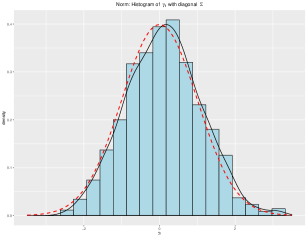
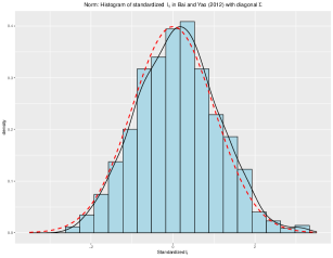
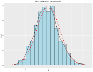
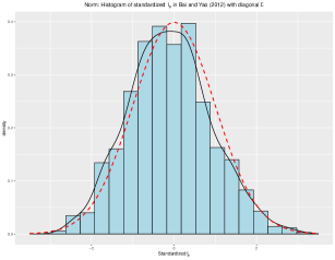
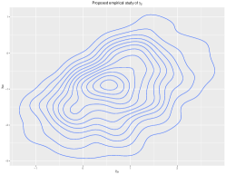
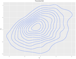
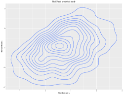
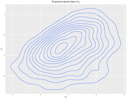
Figure 1: Case I under Gaussian Assumption. Upper two panels show that the histograms of the proposed $\gamma_{1}$ and $\gamma_{4}$ comparing to the ones of standardized $l_{1}$ and $l_{p}$ in Bai and Yao (2012) , as well as the empirical densities (solid lines) and their Gaussian limits (dashed lines). Lower two panels show the contour plots: the left ones are the proposed empirical joint density function of $(\gamma_{i1},\gamma_{i2}),i=2,3.$; the middle ones are their corresponding limits; the right ones are the empirical joint density function of standardized $(l_{2},l_{3})$ and $(l_{p-2},l_{p-1})$.

4.2 Case I under Binomial Assumption

If $\{x_{ij}\}$ are from Binomial Assumption in the Case I, then it is obtained by the Remark 3.2 as below:

• First, for the single population spikes $\alpha_{1}=4$ and $\alpha_{4}=0.1$ , we have :

  $$\gamma_{1}=\sqrt{n}\Big{(}\frac{l_{1}(S)}{\phi_{n,1}}-1\Big{)}\rightarrow N(0,\sigma_{1}^{2})$$

  where $\phi_{n,1}=4.667$, $\sigma_{1}^{2}=0.074$, and

  $$\gamma_{4}=\sqrt{n}\Big{(}\frac{l_{p}(S)}{\phi_{n,4}}-1\Big{)}\rightarrow N(0,\sigma_{4}^{2})$$

  with $\phi_{n,4}=0.044,\sigma_{4}^{2}=2.414.$

• Second, for the spikes $\alpha_{2}=3$ with multiplicity 2, we obtain

  $$\gamma_{2}=\left(\gamma_{21},\gamma_{22}\right)^{\prime}=\left(\sqrt{n}\Big{(}\frac{l_{2}(S)}{\phi_{n,2}}-1\Big{)},\sqrt{n}\Big{(}\frac{l_{3}(S)}{\phi_{n,2}}-1\Big{)}\right)^{\prime}$$

  converges to the eigenvalues of random matrix $-\frac{1}{\kappa_{s}}\left[\Omega_{\phi_{2}}\right]_{22}$, where $\phi_{n,2}=3.750$, $\kappa_{s}=1.417$ for the spike $\alpha_{2}=3$. Furthermore, the matrix $\left[\Omega_{\phi_{2}}\right]_{22}$ is a $2\times 2$ symmetric matrix with the independent Gaussian entries, of which the $(i,j)$ element has mean zero and the variance given by

  $$var(w_{ij})=\left\{\begin{array}[]{cc}0.263,&~{}\text{if}~{}i=j\\ 1.131,&~{}\text{if}~{}i\neq j\end{array}\right.$$

  Similarly, for the spikes $\alpha_{3}=0.2$ with multiplicity 2,

  $$\gamma_{3}=\left(\gamma_{31},\gamma_{32}\right)^{\prime}=\left(\sqrt{n}\Big{(}\frac{l_{p-2}(S)}{\phi_{n,3}}-1\Big{)},\sqrt{n}\Big{(}\frac{l_{p-1}(S)}{\phi_{n,3}}-1\Big{)}\right)^{\prime}$$

  converges to the eigenvalues of random matrix $-\frac{1}{\kappa_{s}}\left[\Omega_{\phi_{3}}\right]_{33}$, where $\phi_{n,3}=0.075$, $\kappa_{s}=1.649$ for the spike $\alpha_{3}=0.2$. Furthermore, the matrix $\left[\Omega_{\phi_{3}}\right]_{33}$ is a $2\times 2$ symmetric matrix with the independent Gaussian entries, of which the $(i,j)$ element has mean zero and the variance given by

  $$var(w_{ij})=\left\{\begin{array}[]{cc}4.481,&~{}\text{if}~{}i=j\\ 6.873,&~{}\text{if}~{}i\neq j\end{array}\right.$$

The simulated empirical distributions of the spiked eigenvalues from Binomial Assumption under Case I are drawn in Figure 2 in contrast to their corresponding limiting distributions.

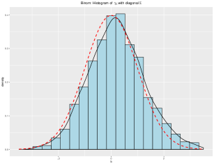
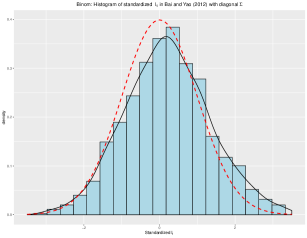
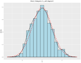
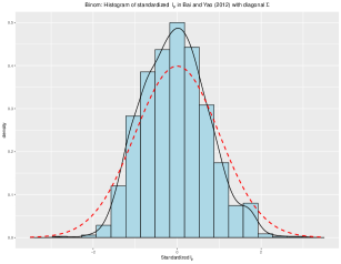
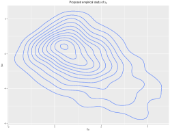
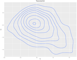
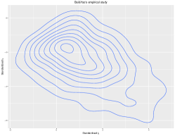
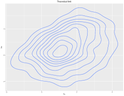
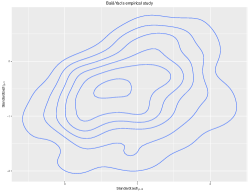
Figure 2: Case I under Binomial Assumption.

As shown in the simulations of the Case I, our approach provides the similar results to the ones in Bai and Yao (2012), when the population covariance matrix has a diagonal structure. Moreover, our method performs slightly better for the non-Gaussian distribution even if the diagonal independent assumption holds in the Case I.

4.3 Case II under the both Assumptions

For the Case II, it is easily obtained by Theorem 3.1 that our proposed results of the both population assumptions are the same to the one of Gaussian Assumption in Case I, which can well fit their corresponding limiting behaviors. However, as shown in the simulated results, the asymptotic distribution in Bai and Yao (2012), which is involved with the 4th moment, performs not well for the non-Gaussian population assumption in the Case II. Therefore, it is reasonable to theoretically remove the diagonal independent restrictions in results of Bai and Yao (2008,2012) as illustrated in the simulations. The simulated results of the two population assumptions in Case II are respectively depicted in Figures 3 and 4.

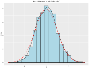
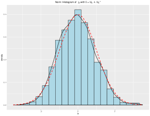
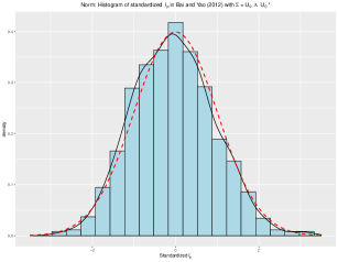
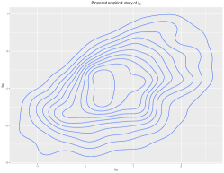
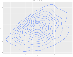
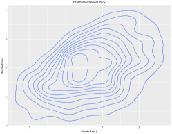
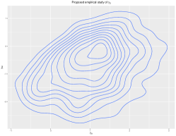
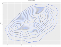
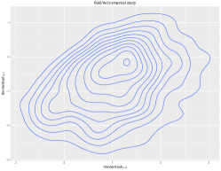
Figure 3: Case II under Gaussian assumption.

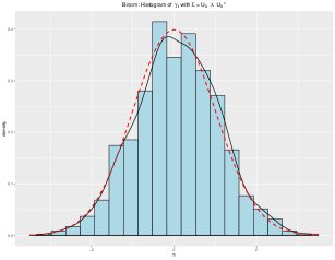
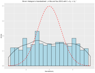
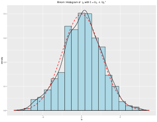
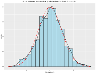
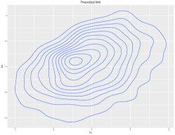
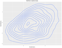
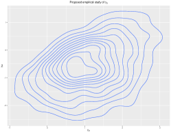
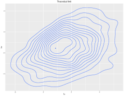
Figure 4: Case II under Binomial assumption.

5 Applications and real data analysis

5.1 Application to determine the number of the spikes.

Since the spiked model is closely related to principal component analysis, it has important applications to the statistical inferences in many scientific fields. For example, to reconstruct the original signals in wireless communication, to rebuild the observed assets into a low-dimensional set of unobserved variables, which are the factors in economics, and so on. One of the basic but important statistical inferences in these applications is to determine the number of principal components / signals / factors, that is, the number of spiked eigenvalues.

As mentioned in (1.1), the population eigenvalues are

$$\beta_{p,1},\cdots,\beta_{p,j},\cdots,\beta_{p,p},$$ (5.1)

where $\beta_{p,j_{k}+1},\cdots\beta_{p,j_{k}+m_{k}}=\alpha_{k}$, $k=1,\cdots,K$ are the spikes with multiplicity $m_{k},k=1,\cdots,K$, and $m_{1}+\cdots+m_{K}=M$ is a fixed but unknown number.

We propose to estimate the number of the spikes, $M$, by our result in Theorem 3.1. First, for every sample eigenvalue $l_{j}$, $j\in J_{k}$, it follows from Theorem 3.1 that

$$\sqrt{n}\Big{(}\frac{l_{j}(S)}{\phi_{n,k}}-1\Big{)}\bigg{/}\sigma_{k}\sim\mathcal{N}(0,1)$$

where $\sigma_{k}^{2}=2\theta_{k}/\kappa_{s}^{2}$ under our Assumption A $\sim$ E and $\sigma_{k}^{2}=(2\theta_{k}+\beta_{x}\nu_{k})/\kappa_{s}^{2}$ under the assumptions of the diagonal or diagonal block independence with the bounded spikes and the 4th moments. Then, for every sample eigenvalue $l_{j}$, we can calculate an corresponding interval

$$C_{j}=\left[\big{(}\frac{z_{0.05}\sigma_{k}}{\sqrt{n}}+1\big{)}\phi_{k},\quad\big{(}\frac{z_{0.95}\sigma_{k}}{\sqrt{n}}+1\big{)}\phi_{k}\right],$$

where $z_{0.05},z_{0.95}$ are the 5% and 95% quantiles of the standard normal distribution. If $l_{j}\in C_{j}$, then it is concluded that the population eigenvalues in according to $l_{j}$ is a spike; Otherwise, it is not a spike. Similarly, the same procedures are conducted for all the sample eigenvalues, and consequently a sequence of intervals $\{C_{j},j=1,\cdots,p\}$ are obtained. Therefore, we propose an estimator for the number of the spikes, $M$, as follows

$$\hat{M}_{0}=\sum\limits_{j=1}^{p}I_{(l_{j}\in C_{j})}$$

where $I(\cdot)$ is the indicator function.

However, $\phi_{k}$ in (2.4) and $\sigma_{k}^{2}$ calculated by Theorem 3.1 or Remark 3.1 cannot be directly obtained by their expressions in practice, because they are involved with the unknown population spikes $\alpha_{k},k=1,\cdots,K$. Therefore, we provide some estimations to get the estimated interval $\hat{C}_{j}$, and then

$$\hat{M}_{0}=\sum\limits_{j=1}^{p}I_{(l_{j}\in\hat{C}_{j})}$$

which is feasible in practice.

First, by the first equation in (3.6), it asymptotically holds that

$$l_{j}+l_{j}\underline{m}(l_{j})\alpha_{k}=0.$$

So we use $-\displaystyle\frac{1}{\underline{m}(l_{j})}$ to estimate $\alpha_{k}$, where $\underline{m}(\cdot)$ defined in (3.9) is the Stieltjes transform of the LSD of the matrix $\frac{1}{n}{\bf X}^{*}\Gamma{\bf X}$. Since the number of spikes is fixed, the LSD of $\displaystyle\frac{1}{n}{\bf X}^{*}\Gamma{\bf X}$ is approximately the same as the one of the matrix $\displaystyle\frac{1}{n}{\bf X}^{*}UDU^{*}{\bf X}$, where $D={\rm diag}(D_{1},D_{2})$. Therefore, we further define $r_{ij}=|l_{i}-l_{j}|/\max(l_{i},l_{j})$ and adopt

$$\hat{m}(l_{j})=\frac{1}{p}\sum\limits_{r_{ij}\geq 0.2;i=1}^{p}(l_{i}-l_{j})^{-1},$$

which is a good estimator of $m(l_{j})$, and $m(\cdot)$ is the Stieltjes transform of the LSD of the matrix $\displaystyle\frac{1}{n}D_{2}^{1/2}U_{2}^{*}{\bf X}{\bf X}^{*}U_{2}D_{2}^{1/2}$. The setting $\{i\in(1,\cdots,p):r_{ij}\geq 0.2\}$ is selected to avoid the effect of multiple roots, which makes the estimations of the population spikes inaccurate. The constant 0.2 is a more suitable threshold value of the ratio based on our simulated results, but for other different populations, the appropriate threshold can be selected by simulation experiments, which is about 10% to 30%. Moreover, by the equation

$$\underline{m}(l_{j})=-\displaystyle\frac{1-c}{l_{j}}+cm(l_{j})$$

we obtain the estimator of $\underline{m}(l_{j})$ as below

$$\hat{}\underline{m}(l_{j})=-\displaystyle\frac{1-c}{l_{j}}+c\hat{m}(l_{j})$$

Finally, we obtain the estimator of $\alpha_{k}$, which is expressed as $\hat{\alpha}_{k}=-\displaystyle\frac{1}{\hat{}\underline{m}(l_{j})}$. Without extra efforts, the following estimators are automatically obtained that

$$\hat{\phi}_{k}=\phi(\hat{\alpha}_{k});$$ (5.2)

$$\hat{m}(\phi_{k})=\frac{1}{p}\sum\limits_{i=1}^{p}(l_{i}-\hat{\phi}_{k})^{-1};\quad \hat{}\underline{m}(\phi_{k})=-\displaystyle\frac{1-c}{\hat{\phi}_{k}}+c\hat{m}(\hat{\phi}_{k});$$ (5.3)

$$\hat{m}_{2}(\phi_{k})=\frac{1}{p}\sum\limits_{i=1}^{p}(l_{i}-\hat{\phi}_{k})^{-2};\quad \hat{}\underline{m}_{2}(\phi_{k})=\displaystyle\frac{1-c}{\hat{\phi}_{k}^{2}}+c\hat{m}_{2}(\hat{\phi}_{k});$$ (5.4)

So the estimators of $\sigma_{k},\phi_{k}$ for the renewal interval $\hat{C}_{j}$ can be expressed by the above estimations.

Through our approach, not only can we estimate the number of the spikes more accurately, but we can also give the estimations of the population spikes, as well as the limits of the sample spiked eigenvalues. More importantly, we can also provide the specific locations of these spikes.

5.2 Numerical results for Section 5.1

For the two cases of $\Sigma$ designed in Section 4 with $M=6$, we use the method provided in Section 5.1 to estimate the number of the population spikes under different population assumptions in Section 4.

To evaluate the performance of our approach, we shall compare it with some existing methods. Since the method in Onatski (2009) provides a better estimator than that in Bai and Ng (2002), and Cai, et al. (2019) shows that their approach performs better than that in both of Onatski (2009) and Bai, et al. (2018), so we only consider the procedure proposed in Cai, et al. (2019) and the method introduced by Passemier and Yao (2012), which are simply denoted as CHP and PY, respectively.

The following tables report the estimator of the number of the spikes and its corresponding frequency by three methods. As shown in the tables, our method can give an accurate estimate of the number of the spikes in a large probability, while the other two methods fail to detect the very small spikes because they both assume that the population spikes are the larger eigenvalues, satisfying that $\alpha_{1}\geq\alpha_{2}\geq\cdots\geq\alpha_{M}\geq\beta_{1}\geq\cdots\geq\beta_{p-M}$. However, it makes sense to detect all the spiked eigenvalues, including the minimal ones. For example, the original system with all the same eigenvalues has changed after the input of some signals. If we want to test which positions in the system have changed, then it is equivalent to finding out all the spiked eigenvalues. In addition, our method has an advantage over other methods, that is, it also presents the the estimations of the population spikes, and the specific locations of these spikes in the tables.

Table 1: Estimations of the number of the population spikes and its frequency.

Case I under Gaussian Assumption
			Frequency of $\hat{M}_{0}$
	$\hat{M}_{0}$	1	2	3	4	5	6	7
$p$=200	Ours	0	0	0	0	0.024	0.943	0.033
$n$=1000	CHP	0	0	0	1	0	0	0
	PY	0.358	0	0.642	0	0	0	0
$p$=400	Ours	0	0	0	0	0.027	0.928	0.045
$n$=1000	CHP	0	0	0	1	0	0	0
	PY	0.371	0	0.629	0	0	0	0

Case I under Binomial Assumption
			Frequency of $\hat{M}_{0}$
	$\hat{M}_{0}$	1	2	3	4	5	6	7
$p$=200	Ours	0	0	0	0	0.054	0.943	0.003
$n$=1000	CHP	0	0	0	1	0	0	0
	PY	0.622	0	0.378	0	0	0	0
$p$=400	Ours	0	0	0	0.005	0.073	0.910	0.012
$n$=1000	CHP	0	0	0	1	0	0	0
	PY	0.640	0	0.360	0	0	0	0

Table 2: Estimations of the population spikes and its locations by our method.

Case I under Gaussian Assumption
$p$=200; $n$=1000	Estimation of the location of the population spikes
	(1, 2, 3,  198, 199, 200)
	Estimation of the population spikes
	$\hat{\alpha}_{1}$	$\hat{\alpha}_{2}$	$\hat{\alpha}_{3}$	$\hat{\alpha}_{4}$	$\hat{\alpha}_{5}$	$\hat{\alpha}_{6}$
	3.993	3.207	3.014	0.202	0.198	0.098
$p$=400; $n$=1000	Estimation of the location of the population spikes
	(1, 2, 3,  198, 199, 200)
	Estimation of the population spikes
	$\hat{\alpha}_{1}$	$\hat{\alpha}_{2}$	$\hat{\alpha}_{3}$	$\hat{\alpha}_{4}$	$\hat{\alpha}_{5}$	$\hat{\alpha}_{6}$
	3.930	3.052	3.015	0.206	0.186	0.117

Case I under Binomial Assumption
$p$=200; $n$=1000	Estimation of the location of the population spikes
	(1, 2, 3,  198, 199, 200)
	Estimation of the population spikes
	$\hat{\alpha}_{1}$	$\hat{\alpha}_{2}$	$\hat{\alpha}_{3}$	$\hat{\alpha}_{4}$	$\hat{\alpha}_{5}$	$\hat{\alpha}_{6}$
	4.025	3.091	2.951	0.194	0.185	0.099
$p$=400; $n$=1000	Estimation of the location of the population spikes
	(1, 2, 3,  198, 199, 200)
	Estimation of the population spikes
	$\hat{\alpha}_{1}$	$\hat{\alpha}_{2}$	$\hat{\alpha}_{3}$	$\hat{\alpha}_{4}$	$\hat{\alpha}_{5}$	$\hat{\alpha}_{6}$
	4.018	3.008	2.876	0.207	0.194	0.101

Table 3: Estimations of the number of the population spikes and its frequency.

Case II under Gaussian Assumption
			Frequency of $\hat{M}_{0}$
	$\hat{M}_{0}$	1	2	3	4	5	6	7
$p$=200	Ours	0	0	0	0	0.019	0.950	0.031
$n$=1000	CHP	0	0	0	1	0	0	0
	PY	0.375	0	0.625	0	0	0	0
$p$=400	Ours	0	0	0	0	0.025	0.927	0.048
$n$=1000	CHP	0	0	0	1	0	0	0
	PY	0.356	0	0.644	0	0	0	0

Case II under Binomial Assumption
			Frequency of $\hat{M}_{0}$
	$\hat{M}_{0}$	1	2	3	4	5	6	7
$p$=200	Ours	0	0	0	0	0.018	0.980	0.002
$n$=1000	CHP	0	0	0	1	0	0	0
	PY	0.343	0	0.657	0	0	0	0
$p$=400	Ours	0	0	0	0	0.041	0.952	0.007
$n$=1000	CHP	0	0	0	1	0	0	0
	PY	0.374	0.001	0.625	0	0	0	0

Table 4: Estimations of the population spikes and its locations by our method.

Case II under Gaussian Assumption
$p$=200; $n$=1000	Estimation of the location of the population spikes
	(1, 2, 3,  198, 199, 200)
	Estimation of the population spikes
	$\hat{\alpha}_{1}$	$\hat{\alpha}_{2}$	$\hat{\alpha}_{3}$	$\hat{\alpha}_{4}$	$\hat{\alpha}_{5}$	$\hat{\alpha}_{6}$
	4.080	3.122	2.909	0.208	0.191	0.010
$p$=400; $n$=1000	Estimation of the location of the population spikes
	(1, 2, 3,  198, 199, 200)
	Estimation of the population spikes
	$\hat{\alpha}_{1}$	$\hat{\alpha}_{2}$	$\hat{\alpha}_{3}$	$\hat{\alpha}_{4}$	$\hat{\alpha}_{5}$	$\hat{\alpha}_{6}$
	3.949	3.217	2.887	0.231	0.188	0.102

Case II under Binomial Assumption
$p$=200; $n$=1000	Estimation of the location of the population spikes
	(1, 2, 3,  198, 199, 200)
	Estimation of the population spikes
	$\hat{\alpha}_{1}$	$\hat{\alpha}_{2}$	$\hat{\alpha}_{3}$	$\hat{\alpha}_{4}$	$\hat{\alpha}_{5}$	$\hat{\alpha}_{6}$
	3.838	3.275	2.922	0.216	0.192	0.098
$p$=400; $n$=1000	Estimation of the location of the population spikes
	(1, 2, 3,  198, 199, 200)
	Estimation of the population spikes
	$\hat{\alpha}_{1}$	$\hat{\alpha}_{2}$	$\hat{\alpha}_{3}$	$\hat{\alpha}_{4}$	$\hat{\alpha}_{5}$	$\hat{\alpha}_{6}$
	4.123	3.211	3.001	0.216	0.195	0.096

5.3 Real data analysis

Now we apply the procedure of determining the number of the spikes proposed in Section 5.1 to the actual data titled as ”Early stage of Indians Chronic Kidney Disease(CKD)”.

The data came from records collected by a hospital in India over a period of about 2 months, which consists of 400 observations and 25 variables. The first 24 variables $X_{1}\cdots,X_{24}$ are independent variables, which rerecord the various laboratory indicators and hospital records, including age, blood pressure (bp), specific gravity (sg), albumin (al), sugar (su), red blood cells (rbc), pus cell (pc), pus cell clumps (pcc), bacteria (ba), blood glucose random (bgr), blood urea (bu), serum creatinine (sc), sodium (sod), potassium (pot), hemoglobin (hemo), packed cell volume (pcv), white blood cell count (wc), red blood cell count (rc), hypertension (htn), diabetes mellitus (dm), coronary artery disease (cad), appetite (appet), pedal edema (pe), anemia (ane). The 25th variable is the dependent variable to indicate whether the patient has chronic kidney disease(ckd).

We apply our method to determine the number of the spikes of the covariance matrix $\Sigma_{0}$ generated from the standardized data of the first 24 variables with 114 observations (For simplicity, we have only chosen 114 observations without missing values). Then, we obtain the following results in the Table 5.

Table 5: Estimations of the number, the sizes and the location of the population spikes by using the real data.

Number:	9
Location:	(1, 2,  18, 19, 20, 21,  22,  23,  24)
Sizes:	$\hat{\alpha}_{1}$	$\hat{\alpha}_{2}$	$\hat{\alpha}_{3}$	$\hat{\alpha}_{4}$	$\hat{\alpha}_{5}$	$\hat{\alpha}_{6}$	$\hat{\alpha}_{7}$	$\hat{\alpha}_{8}$	$\hat{\alpha}_{9}$
	10.818	2.143	0.219	0.166	0.124	0.101	0.064	0.048	0.009

As seen from the Table 5, if we define the singular value decomposition of $\Sigma_{0}$ as $\Sigma_{0}=U\Lambda_{0}U^{\prime}$, and ${\bf u}_{i}$ is the $i$th column of the orthogonal matrix $U$, then the factors generated from independent variables $X=(X_{1}\cdots,X_{24})^{\prime}$ can be roughly divided into three groups: one group has a greater impact with larger spiked eigenvalues, like ${\bf u}^{\prime}_{1}X,{\bf u}^{\prime}_{2}X$; Another group of much weaker effects, like ${\bf u}^{\prime}_{i}X$, $i=18,\cdots,24$; The last group that may have most of the same effects, like ${\bf u}^{\prime}_{i}X$, $i=3,\cdots,17$. Furthermore, if we use the data with the missing values made up, the experimental results may be more accurate. To make up for missing values, one can use the missForest function in the package missForest.

6 Conclusion

In this paper, we propose a G4MT for a generalized spiked covariance matrix, which shows the universality of the asymptotic law for its spiked eigenvalues. Through the concrete example of the CLT of normalized spiked eigenvalues, we illustrate the basic idea and procedures of the G4MT to show the universality of a limiting result related to the large dimensional random matrices. Unlike Tao and Vu (2015), we avoid the estimates of high-order partial derivatives of an implicit function to the entries of the random matrix, and thus, the strong condition $C_{0}$ of sub-exponential property is avoided. Moreover, the required 4th moment condition is reduced to a tail probability in Assumption ${\bf B}$, which is necessary for the existence of the largest eigenvalue limit. Without the constraint of the existence of the 4th moment, we only need a more regular and minor condition (2.3) on the elements of $U_{1}$. On the one hand, our result has much wider applications than Bai and Yao (2008, 2012); on the other hand, the result of Bai and Yao (2012) shows the necessity of the condition (2.3).

Supplement to ”Generalized Four Moment Theorem and an Application to CLT for Spiked Eigenvalues of high-dimensional Covariance Matrices”.

A The detailed explanation of Assumption D

For the Assumption D, we have

Remark A.1.

In the proof of the main theorems, this assumption is actually used as

$$\max\limits_{t,s}|u_{ts}|^{2}\big{(}{\rm E}|x_{11}|^{4}-3\big{)}I(|x_{11}|<\eta_{n}\sqrt{n})\rightarrow 0,$$

where $\eta_{n}\to 0$ with a slow rate. In fact, because of Assumption ${\bf B}$, the condition (2.3) remains the same as

$$\max\limits_{t,s}|u_{ts}|^{2}\big{(}{\rm E}|x_{11}|^{4}-3\big{)}I(|x_{11}|<\eta\sqrt{n})\rightarrow 0,$$

provided $|\log\eta|<1/4\log n$.

Remark A.2.

If the 4th moment of population random variable $X$ is bounded, only the condition

$$\max\limits_{t,s}|u_{ts}|^{2}\rightarrow 0$$

is needed; if the 4th moment does not exist, we only need

$$\max\limits_{t,s}|u_{ts}|^{2}=O({\log^{-1}n})$$

at most, since the 4th moment of the truncated variables is $o(\log n)$ by Lemma C.1.

For example, assume that the random variable $X$ follows the population distribution with the density

$$d(x)=\frac{a_{0}}{\big{(}|x|+1\big{)}^{5}\log{\big{(}|x|+2\big{)}}},$$

where $a_{0}$ is a scaling number; then,

$${\rm P}\left(|X|>x\right) =O\left(|x|^{-4}\log^{-1}{\big{(}|x|+2\big{)}}\right),$$

which implies

$${\rm E}|X|^{4}I(|X|>\eta_{n}\sqrt{n})=O\big{(}\log(\log n)\big{)}$$

Then, the condition (2.3) can be reduced to a weaker one, i.e.

$$\max\limits_{t,s}|u_{ts}|^{2}=o\big{(}1/\log(\log n)\big{)}.$$

B Proof of the Truncation and Centralization

By the Assumption ${\bf B}$, let $\tau=\eta\sqrt{n}\rightarrow\infty$; for every fixed $\eta>0$, we obtain that

$$\eta^{4}n^{2}{\rm P}\left(|x_{ij}|>\eta\sqrt{n}\right)\rightarrow 0.$$

The limiting behavior still performs well by removing the fixed $\eta^{4}$, that is,

$$n^{2}{\rm P}\left(|x_{ij}|>\eta\sqrt{n}\right)\rightarrow 0.$$ (B.1)

Because of the arbitrariness of $\eta$ in (B.1), it is proved by Lemma 15 in Li, et al. (2016) that there exist a sequence of positive numbers $\eta=\eta_{n}\to 0$ such that

$$n^{2}{\rm P}\left(|x_{ij}|>\eta_{n}\sqrt{n}\right)\rightarrow 0.$$ (B.2)

The convergence rate of the constants $\eta_{n}$ can be selected arbitrarily slowly, and hence, we may assume that $\eta_{n}n^{1/5}\rightarrow\infty$.

Then, consider the truncated samples $\hat{x}_{ij}=x_{ij}{\rm I}(|x_{ij}|<\eta_{n}\sqrt{n})$, set

$${\bf r}_{j}=\frac{1}{\sqrt{n}}T_{p}{\bf x}_{j},\quad\hat{\bf r}_{j}=\frac{1}{\sqrt{n}}T_{p}\hat{\bf x}_{j}$$

where $T_{p}T_{p}^{*}=\Sigma$. Consequently, the generalized spiked sample covariance $S$ is expressed as

$$S=T_{p}\left(\frac{1}{n}{\bf X}{\bf X}^{*}\right)T_{p}^{*}=\sum\limits_{j=1}^{n}{\bf r}_{j}{\bf r}_{j}^{*}:={\bf R}_{n}{\bf R}_{n}^{*}.$$

Define the matrix with truncated entries as

$$\hat{S}=\sum\limits_{j=1}^{n}\hat{\bf r}_{j}\hat{\bf r}_{j}^{*}:=\hat{\bf R}_{n}\hat{\bf R}_{n}^{*}.$$

Therefore, according to the property (B.2), we have

$${\rm P}\left(S\neq\hat{S}\right)={\rm P}\left(\sum\limits_{j=1}^{n}{\bf r}_{j}{\bf r}_{j}^{*}\neq\sum\limits_{j=1}^{n}\hat{\bf r}_{j}\hat{\bf r}_{j}^{*}\right)$$

$$\leq\sum\limits_{i,j}{\rm P}\left(|x_{ij}|\geq\eta_{n}\sqrt{n}\right)=np{\rm P}\left(|x_{11}|\geq\eta_{n}\sqrt{n}\right)\rightarrow 0,\quad\text{as }n,p\rightarrow\infty.$$

Next, define the truncated and centralized sample covariance matrix as

$$\tilde{S}=\sum\limits_{j=1}^{n}\tilde{\bf r}_{j}\tilde{\bf r}_{j}^{*}:=\tilde{\bf R}_{n}\tilde{\bf R}_{n}^{*},$$

where $\tilde{\bf r}_{j}=T_{p}\tilde{\bf x}_{j}/\sqrt{n}$ and $\tilde{x}_{ij}=(\hat{x}_{ij}-{\rm E}\hat{x}_{ij})/\sigma_{n}$ with $\sigma_{n}^{2}={\rm E}\left|\hat{x}_{ij}-{\rm E}\hat{x}_{ij}\right|^{2}$. Then, by Theorem A.46 of Bai and Silverstein (2010), we have

$$\max\left\{l_{j}^{1/2}(\tilde{S})-l_{j}^{1/2}(\hat{S})\right\}\leq\|\tilde{\bf R}_{n}-\hat{\bf R}_{n}\|=\|{\rm E}\hat{\bf R}_{n}\|+\|(1-\sigma_{n})\tilde{\bf R}_{n}\|$$

$$\leq n^{-1/2}|{\rm E}\hat{x}_{11}|\min(p,n)+\frac{1-\sigma_{n}^{2}}{1+\sigma_{n}}\|\tilde{\bf R}_{n}\|$$

$$= o_{a.s}(n^{-1}),$$

where we have used the fact that there exists a finite constant $C_{0}$ such that $|{\rm E}\hat{x}_{11}|\leq C_{0}\int^{+\infty}_{\eta_{n}\sqrt{n}}P(|x_{11}|\geq x)\mbox{d}x=o(n^{-3/2})$, and that $1-\sigma_{n}^{2}={\rm E}x_{11}^{2}I(|x_{11}|\geq\eta_{n}\sqrt{n})+{\rm E}x^{2}_{11}I(|x_{11}|<\eta_{n}\sqrt{n})=o(n^{-1})$ in Lemma C.1 and $\|\hat{\bf R}_{n}\|\leq\|T_{p}\|(1+\sqrt{c}+\varepsilon),a.s.$.

Thus, it is concluded that the procedure of centralization does not have an effect on the limiting distribution of the spiked eigenvalues because of

$$\sqrt{n}\left\{\frac{l_{j}(\tilde{S})}{\phi_{n,k}}-1-\left(\frac{l_{j}(\hat{S})}{\phi_{n,k}}-1\right)\right\}\leq o(\phi_{n,k}^{-1}n^{-{\frac{1}{2}}}).$$

C Lemmas

Some useful lemmas are provided in this section, which are needed to prove the Theorem 3.2. First, we investigate the arbitrary moments of $\ \tilde{x}_{ij}$ and depict their convergence rates in the following lemma.

Lemma C.1.

For the entries $\{\tilde{x}_{ij}\}$ truncated at $\eta_{n}\sqrt{n}$, centralized and renormalized, it follows that

$$|{\rm E}\tilde{x}_{ij}^{\alpha}|\leq o(\sqrt{n})^{\alpha-4},~{}\alpha>4;$$

$$|{\rm E}\tilde{x}_{ij}^{\alpha}|=o(\log n),~{}\alpha=4;$$

$$|{\rm E}\tilde{x}_{ij}^{\alpha}|\leq o(\sqrt{n})^{\alpha-4},~{}\alpha<4;$$

Proof.

We only estimate the inequalities above with $\tilde{x}_{ij}$ replaced by $\hat{x}_{ij}$ because the centralization only involves the third estimate with $\alpha=1$. For any integer $\alpha<4$, we have

$$|{\rm E}\hat{x}_{ij}^{\alpha}| = \int_{\eta_{n}\sqrt{n}}^{\infty}\alpha x^{\alpha-1}P(|x_{ij}|>x)dx$$

$$\leq \int_{\eta_{n}\sqrt{n}}^{\infty}o(x^{\alpha-5})dx=o((\eta_{n}\sqrt{n})^{\alpha-4}).$$

Therefore, $|{\rm E}\hat{x}_{ij}^{\alpha}|\leq o(\sqrt{n})^{\alpha-4}$, if $\alpha<4$.

For the case of $\alpha=4$, we have

$$|{\rm E}\hat{\bf x}_{i}^{4}| = \int_{0}^{\eta_{n}\sqrt{n}}x^{4}\mbox{d}P(|x_{ij}|\leq x)$$

$$= -\int_{0}^{\eta_{n}\sqrt{n}}x^{4}\mbox{d}P(|x_{ij}|>x)\leq\int_{0}^{\eta_{n}\sqrt{n}}4x^{3}P(|x_{ij}|>x)dx$$

$$\leq O(1)+\int_{K}^{\eta_{n}\sqrt{n}}4x^{3}o(x^{-4})\mbox{d}x=o(\log n).$$

For any integer $\alpha>4$,

$${\rm E}|\hat{\bf x}_{i}^{\alpha}| = \int_{0}^{\eta_{n}\sqrt{n}}x^{\alpha}\mbox{d}P_{x}(|x_{ij}|\leq x)$$

$$\leq \alpha\int_{0}^{\eta_{n}\sqrt{n}}x^{\alpha-1}P(|x_{ij}|>x)\mbox{d}x=o(\sqrt{n}^{\alpha-4})$$

∎

Second, before proceeding with the proof of the G4MT numbered as Theorem 3.2, we begin with some preliminary lemmas used during the process.

Lemma C.2.

Let ${{\bf X}}=({\bf x}_{1},\cdots,{\bf x}_{n})$ and ${\bf Y}=({\bf y}_{1},\cdots,{\bf y}_{n})$ be two independent random matrices satisfying Assumptions ${\bf A}\sim{\bf E}$, and set ${\bf X}_{k}=({\bf x}_{1},\cdots,{\bf x}_{k},$ ${\bf y}_{k+1},\cdots,{\bf y}_{n})$ with convention ${\bf X}={\bf X}_{n}$ and ${\bf Y}={\bf X}_{0}$. Denote ${\bf X}_{k0}=({\bf x}_{1}\cdots,\!{\bf x}_{k\!-\!1},$ ${\bf y}_{k+1}\cdots{\bf y}_{n})$,

$$\beta_{k}=1-n^{-1}{\bf x}_{k}^{*}\Gamma^{1/2}(\lambda{\bf I}_{p}-n^{-1}\Gamma^{1/2}{\bf X}_{k0}{\bf X}_{k0}^{*}\Gamma^{1/2})^{-1}\Gamma^{1/2}{\bf x}_{k}.$$

and

$$\beta_{k0}=1-n^{-1}{\rm tr}\Big{(}\Gamma(\lambda{\bf I}_{p}-n^{-1}\Gamma^{1/2}{\bf X}_{k0}{\bf X}_{k0}^{*}\Gamma^{1/2})^{-1}\Big{)}.$$

with $\Gamma=U_{2}D_{2}U^{*}_{2}$ defined in (3.5). Then, it is obtained that

$$\beta_{k0} \to -\frac{1}{\lambda\underline{m}(\lambda)}\neq 0$$

$$\varepsilon_{k} = \beta_{k}-\beta_{k0}\to 0$$

$${\rm E}_{k}\varepsilon^{2}_{k} \leq o(n^{-1}\log n)$$

$${\rm E}_{k}\varepsilon_{k}^{4} = o(n^{-1}),$$

where $\underline{m}(\lambda)$ is the Stieltjes transform of the LSD of the matrix $\displaystyle\frac{1}{n}{\bf X}_{k0}^{*}\Gamma{\bf X}_{k0}$, ${\rm E}_{0}(\cdot)$ denotes the expectation and ${\rm E}_{k}(\cdot)$ denotes the conditional expectation with respect to the $\sigma$-field generated by the vectors ${\bf x}_{1},\cdots,{\bf x}_{k}$.

Proof.

Denote $m(\lambda,{\bf X}_{k0})$ and $\underline{m}(\lambda,{\bf X}_{k0})$ as the Stieltjes transforms of the LSDs of the matrix $n^{-1}\Gamma^{1/2}{\bf X}_{k0}{\bf X}_{k0}^{*}\Gamma^{1/2}$ and $\displaystyle\frac{1}{n}{\bf X}_{k0}^{*}\Gamma{\bf X}_{k0}$, respectively. If no confusion, we still use the notations $m(\lambda)$ and $\underline{m}(\lambda)$ for simplicity.

By (3.11), (3.13) and the limitation above (3.14) in Bai and Zhou (2008), we have

$$\frac{1}{n}{\rm tr}\Big{(}\Gamma(\lambda{\bf I}_{p}-n^{-1}\Gamma^{1/2}{\bf X}_{k0}{\bf X}_{k0}^{*}\Gamma^{1/2})^{-1}\Big{)}\sim 1-\frac{1}{1-c-c\lambda m(\lambda)},$$

and it follows that

$$\beta_{k0}=1-n^{-1}{\rm tr}\Big{(}\Gamma(\lambda{\bf I}_{p}-n^{-1}\Gamma^{1/2}{\bf X}_{k0}{\bf X}_{k0}^{*}\Gamma^{1/2})^{-1}\Big{)}\sim-\frac{1}{\lambda\underline{m}(\lambda)}\neq 0.$$

due to the relationship $\underline{m}(\lambda)=-\displaystyle\frac{1-c}{\lambda}+cm(\lambda)$.

The second conclusion $\varepsilon_{k}=\beta_{k}-\beta_{k0}\to 0$ is an easy consequence of the third, ${\rm E}_{k}|\varepsilon_{k}|^{2}\to 0$.

By the formula (1.15) of Bai and Silverstein (2004), we have

$${\rm E}_{k}|\varepsilon_{k}|^{2}=\frac{1}{n^{2}}{\rm E}_{k}\bigg{|}x_{k}^{*}\Gamma^{1/2}(\lambda I_{p}-n^{-1}\Gamma^{1/2}{\bf X}_{k0}{\bf X}_{k0}^{*}\Gamma^{1/2})^{-1}\Gamma^{1/2}x_{k}$$

$$\quad\quad\quad\quad\quad-{\rm tr}\Big{(}\Gamma(\lambda{\bf I}_{p}-n^{-1}\Gamma^{1/2}{\bf X}_{k0}{\bf X}_{k0}^{*}\Gamma^{1/2})^{-1}\Big{)}\bigg{|}^{2}$$

$$=\!\frac{1}{n^{2}}\!\left\{\!{\rm E}_{k}{\rm tr}B^{2}+{\rm E}_{k}{\rm tr}BB^{T}|{\rm E}x_{11}^{2}|^{2}+\sum\limits_{i}{\rm E}_{k}|b_{ii}|^{2}({\rm E}|x_{ik}^{4}|-2-|{\rm E}x_{11}^{2}|^{2})\right\}$$

$$\quad\quad\leq\frac{2}{n^{2}}{\rm E}_{k}{\rm tr}\left[B^{2}\right]+\frac{o(\log n)}{n^{2}}\sum\limits_{i}{\rm E}_{k}|b_{ii}|^{2}\to 0,$$ (C.1)

where $B=\left(b_{ij}\right):=\Gamma^{1/2}(\lambda{\bf I}_{p}-n^{-1}\Gamma^{1/2}{\bf X}_{k0}{\bf X}_{k0}^{*}\Gamma^{1/2})^{-1}\Gamma^{1/2}$, and the eigenvalues of $\Gamma$ are non-spiked eigenvalues and bounded. Then, the third conclusion is proved.

Furthermore, for the conditional moments of $\varepsilon_{k}$, we have

$${\rm E}_{k}\varepsilon^{2}_{k}=o(n^{-1}\log n),$$

which is automatically obtained by equation (C.1).

Finally,

$${\rm E}_{k}\varepsilon_{k}^{4}=\frac{1}{n^{4}}{\rm E}_{k}\bigg{\{}x_{k}^{*}\Gamma^{1/2}(\lambda I_{p}-n^{-1}\Gamma^{1/2}{\bf X}_{k0}{\bf X}_{k0}^{*}\Gamma^{1/2})^{-1}\Gamma^{1/2}x_{k}$$

$$-{\rm tr}\Big{(}\Gamma(\lambda{\bf I}_{p}-n^{-1}\Gamma^{1/2}{\bf X}_{k0}{\bf X}_{k0}^{*}\Gamma^{1/2})^{-1}\Big{)}\bigg{\}}^{4}$$

$$=\!\frac{1}{n^{4}}\Bigg{\{}\big{(}{\rm E}|x_{11}|^{8}-4{\rm E}|x_{11}|^{6}+6{\rm E}|x_{11}|^{4}-3\big{)}\sum\limits_{i}b_{ii}^{4}$$

$$+\big{(}4{\rm E}|x_{11}|^{6}-8{\rm E}|x_{11}|^{4}+4\big{)}\sum\limits_{i\neq j}b_{ii}^{2}b_{ij}^{2}+\!\big{(}{\rm E}|x_{11}|^{4})^{2}-2{\rm E}|x_{11}|^{4}+1\big{)}\sum\limits_{i\neq j}b_{ii}^{2}b_{jj}^{2}$$

$$+16({\rm E}|x_{11}|^{4})^{2}\sum\limits_{i\neq j}b_{ij}^{4}+\big{(}{\rm E}|x_{11}|^{4}-1\big{)}\sum\limits_{i\neq i^{\prime}\neq j^{\prime}}b_{ii}^{2}b_{i^{\prime}j}^{2}$$

$$+16{\rm E}|x_{11}|^{4}\!\big{(}\!\!\sum\limits_{i\neq j\neq j^{\prime}}\!\!\!b_{ij}^{2}b_{ij^{\prime}}^{2}\!+\!\!\sum\limits_{i\neq i^{\prime}\neq j^{\prime}}\!\!\!b_{ij}^{2}b_{i^{\prime}j}^{2}\big{)}\!\!+\!\!\sum\limits_{i\neq j\neq i^{\prime}\neq j^{\prime}}\!\!\!\!\Big{(}16(b_{ij}^{2}+b_{i^{\prime}j^{\prime}}^{2})\!+\!b_{ij}b_{i^{\prime}j}b_{i^{\prime}j}b_{i^{\prime}j^{\prime}}\Big{)}\!\!\Bigg{\}}$$

$$=K_{0}\big{(}o(n^{-1})+o(n^{-2}\log n)+o(n^{-3}\log^{2}n)\big{)}=o(n^{-1}),$$

where $K_{0}$ is an absolute constant and may take different values at different appearances. ∎

Lemma C.3.

Let ${\bf u}_{1i}$, $i=1,2,\cdots,N$ be a column vector of $U_{1}$, ${\bf u}_{2i}$ be a unit $p$-vector orthogonal to $U_{1}$, and $\Gamma$ be an nnd $p\times p$ matrix of bounded spectral norm, where $N=O(n)$. Then, there is a constant $\delta\in(0,1/4)$ such that

$$\max_{i\leq N}n^{-1}\lambda|{\bf u}_{1i}^{*}{\bf X}_{n}(\lambda{\bf I}_{n}-n^{-1}{\bf X}_{n}^{*}\Gamma{\bf X}_{n})^{-1}{\bf X}^{*}_{n}{\bf u}_{2i}|\leq 2n^{-\delta},a.s.$$ (C.2)

Proof.

Note that

$$R_{i} = n^{-1}\lambda{\bf u}_{1i}^{*}{\bf X}_{n}(\lambda{\bf I}_{n}-n^{-1}{\bf X}_{n}^{*}\Gamma{\bf X}_{n})^{-1}{\bf X}^{*}_{n}{\bf u}_{2i}$$

$$= \frac{1}{n}\sum_{k=1}^{n}\frac{{\bf u}_{1i}^{*}x_{k}x_{k}^{*}{\bf u}_{2i}}{\beta_{k}}+\frac{1}{n}\sum_{k_{1}\neq k_{2}}\frac{{\bf u}_{1i}^{*}x_{k_{1}}x_{k_{2}}^{*}{\bf u}_{2i}\beta_{k_{1}k_{2}}}{\beta_{k_{1};k_{2}}\beta_{k_{2};k_{1}}-\beta_{k_{1}k_{2}}^{2}}:=J_{1i}+J_{2i}$$

where

$$\beta_{k_{1}k_{2}} = n^{-1}x_{k_{1}}^{*}U_{2}D_{2}^{1/2}G_{k_{1},k_{2}}^{-1}D_{2}^{1/2}U_{2}^{*}x_{k_{2}}$$

$$\beta_{k_{1};k_{2}} = {\color[rgb]{0,0,1}1-n^{-1}x_{k_{1}}^{*}U_{2}D_{2}^{1/2}G^{-1}_{\color[rgb]{1,0,0}k_{1},k_{2}}D_{2}^{1/2}U_{2}^{*}x_{\color[rgb]{1,0,0}k_{1}}}$$

$$G_{k_{1},k_{2}} = \lambda{\bf I}_{p}-n^{-1}D_{2}^{1/2}U_{2}{\bf X}_{k_{1},k_{2}}{\bf X}_{k_{1},k_{2}}U_{2}^{*}D_{2}^{1/2}$$

where ${\bf X}_{k_{1},k_{2}}$ is identical to ${\bf X}$ excluding the $k_{1}$th and $k_{2}$th columns.

Define notations

$${\color[rgb]{0,0,1}\bar{\beta}_{\color[rgb]{1,0,0}k_{1};k_{2}}} = {\color[rgb]{0,0,1}1-n^{-1}{\rm E}{\rm tr}G^{-1}_{\color[rgb]{1,0,0}k_{1},k_{2}}D_{2}^{1/2}U_{2}^{*}U_{2}D_{2}^{1/2},}$$

$${\color[rgb]{0,0,1}\varepsilon_{k_{1};k_{2}}} = {\color[rgb]{0,0,1}n^{-1}x_{k_{1}}^{*}U_{2}D_{2}^{1/2}G_{\color[rgb]{1,0,0}k_{1},k_{2}}^{-1}D_{2}^{1/2}U_{2}^{*}x_{k_{1}}-n^{-1}{\rm E}{\rm tr}G^{-1}_{\color[rgb]{1,0,0}k_{1},k_{2}}D_{2}^{1/2}U_{2}^{*}U_{2}D_{2}^{1/2},}$$

and events

$${\cal E}_{1k} = \{|\varepsilon_{k}|>\delta_{k}/2\},\ \ \ {\cal E}_{2k}=\{|n^{-1/2}{\bf X}_{k0}|>b_{+}\}$$

$${\cal E}_{k_{1},k_{2}} = \{|\beta_{k_{1}k_{2}}|>\delta_{k}/2\},$$

$${\cal E} = \bigcup_{k=1}^{n}{\cal E}_{k}\bigcup_{k_{1}\neq k_{2}}{{\cal E}_{k_{1},k_{2}}}\{\|{\bf X}/\sqrt{n}\|>b_{+}\}\bigcup\{\|G_{k_{1},k_{2}}^{-1}\|>B^{+}\},$$

where $\delta_{k}={\rm E}\beta_{k}$, $b_{+}>(1+\sqrt{c})^{2}$ and $B^{+}$ are large constants.

Referring to the selection of $\lambda$ and checking the proofs of Bai and Silverstein (1998), one may find that

$$P(\|G_{k_{1},k_{2}}^{-1}\|>B^{+}) = o(n^{-t}),$$

$$P(\|{\bf X}/\sqrt{n}\|>b^{+}) = o(n^{-t}),$$

for any given $t>0$.

Employing Lemma 9.1 of Bai and Silverstein (2010), one can prove that

$$P({\cal E}_{1k}) = o(n^{-t}),$$

$$P({\cal E}_{2k}) = o(n^{-t}),$$

$$P({\cal E}_{k_{1},k_{2}}) = o(n^{-t}).$$

Hence, we have

$$P({\cal E})=o(n^{-t}).$$ (C.3)

We next prove that

$$\max_{i}{\rm E}R_{i}I_{{\cal E}^{c}}\leq n^{-\delta},$$ (C.4)

for some constant $\delta\in(0,1/4)$.

In fact,

$$|{\rm E}J_{1i}I_{{\cal E}^{c}}|=\left|\frac{1}{n}\sum_{k=1}^{n}{\rm E}\frac{{\bf u}_{1i}^{*}x_{k}x_{k}^{*}{\bf u}_{2i}}{\beta_{k0}}I_{{\cal E}^{c}}-\frac{1}{n}\sum_{k=1}^{n}{\rm E}\frac{{\bf u}_{1i}^{*}x_{k}x_{k}^{*}{\bf u}_{2i}\varepsilon_{k}}{\beta_{k0}\beta_{k}}I_{{\cal E}^{c}}\right|$$

$$=\left|\frac{1}{n}\sum_{k=1}^{n}{\rm E}\frac{{\bf u}_{1i}^{*}x_{k}x_{k}^{*}{\bf u}_{2i}}{\beta_{k0}}-\frac{1}{n}\sum_{k=1}^{n}{\rm E}\frac{{\bf u}_{1i}^{*}x_{k}x_{k}^{*}{\bf u}_{2i}}{\beta_{k0}}I_{{\cal E}}-\frac{1}{n}\sum_{k=1}^{n}{\rm E}\frac{{\bf u}_{1i}^{*}x_{k}x_{k}^{*}{\bf u}_{2i}\varepsilon_{k}}{\beta_{k0}\beta_{k}}I_{{\cal E}^{c}}\right|$$ (C.5)

$$\leq P({\cal E})+\frac{{K_{0}}}{n}\sum_{k=1}^{n}{\rm E}|{\bf u}_{1i}^{*}x_{k}x_{k}^{*}{\bf u}_{2i}\varepsilon_{k}|$$

$$\leq{K_{0}}n^{-1/2}\log n\leq n^{-\delta},$$

where $K_{0}$ is an absolute constant independent of $i$, and may take different values at different appearances. Here, we remind the reader that the first term in (C) is zero by the assumption that ${\bf u}_{1i}^{*}{\bf u}_{2i}=0$ and the probability of ${\cal E}$ is $O(n^{-1})$ by (C.3).

Next, we have

$$|{\rm E}J_{2i}I_{{\cal E}^{c}}| = \left|\frac{1}{n}\sum_{k_{1}\neq k_{2}}{\rm E}\frac{{\bf u}_{1i}^{*}x_{k_{1}}x_{k_{2}}^{*}{\bf u}_{2i}\beta_{k_{1}k_{2}}}{\beta_{k_{1};k_{2}}\beta_{k_{2};k_{1}}-\beta_{k_{1}k_{2}}^{2}}\right|I_{{\cal E}^{c}}$$

$$\leq \sum_{l=1}^{5}\left|{\rm E}J_{2li}\right|I_{{\cal E}^{c}},$$

where

$$J_{21i} = \frac{1}{n}\sum_{k_{1}\neq k_{2}}\frac{{\bf u}_{1i}^{*}x_{k_{1}}x_{k_{2}}^{*}{\bf u}_{2i}\beta_{k_{1}k_{2}}}{\bar{\beta}^{2}_{\color[rgb]{1,0,0}k_{1};k_{2}}}$$

$$J_{22i} = \frac{1}{n}\sum_{k_{1}\neq k_{2}}\frac{{\bf u}_{1i}^{*}x_{k_{1}}x_{k_{2}}^{*}{\bf u}_{2i}\beta_{k_{1}k_{2}}(\varepsilon_{k_{1};k_{2}}+\varepsilon_{k_{2};k_{1}})}{\bar{\beta}^{3}_{\color[rgb]{1,0,0}k_{1};k_{2}}}$$

$$J_{23i} = \frac{1}{n}\sum_{k_{1}\neq k_{2}}\frac{({\bf u}_{1i}^{*}x_{k_{1}}x_{k_{2}}^{*}{\bf u}_{2i}+{\bf u}_{1i}^{*}x_{k_{2}}x_{k_{1}}^{*}{\bf u}_{2i})\beta_{k_{1}k_{2}}\varepsilon^{2}_{k_{1};k_{2}}}{\bar{\beta}^{3}_{\color[rgb]{1,0,0}k_{1};k_{2}}\beta_{k_{1};k_{2}}}$$

$$J_{24i} = \frac{1}{n}\sum_{k_{1}\neq k_{2}}\frac{{\bf u}_{1i}^{*}x_{k_{1}}x_{k_{2}}^{*}{\bf u}_{2i}\beta_{k_{1}k_{2}}(\varepsilon^{2}_{k_{1};k_{2}}+\varepsilon_{k_{1};k_{2}}\varepsilon_{k_{2};k_{1}}+\varepsilon^{2}_{k_{2};k_{1}})}{\bar{\beta}^{2}_{\color[rgb]{1,0,0}k_{1};k_{2}}\beta_{k_{1};k_{2}}\beta_{k_{2};k_{1}}}$$

$$J_{25i} = \frac{1}{n}\sum_{k_{1}\neq k_{2}}\frac{{\bf u}_{1i}^{*}x_{k_{1}}x_{k_{2}}^{*}{\bf u}_{2i}\beta_{k_{1}k_{2}}^{3}}{\beta_{k_{1};k_{2}}\beta_{k_{2};k_{1}}(\beta_{k_{1};k_{2}}\beta_{k_{2};k_{1}}-\beta_{k_{1}k_{2}}^{2})}$$

By elementary calculation, we have

$$|{\rm E}J_{21i}I_{{\cal E}^{c}}|=|-{\rm E}J_{21i}I_{{\cal E}}|\leq K_{0}P({\cal E})\leq O(n^{-t})$$

because ${\rm E}J_{21i}=0$, which follows from $U_{2}^{*}{\bf u}_{1i}=0$, and hence

$${\rm E}({\bf u}_{1i}^{*}x_{k_{1}}x_{k_{2}}^{*}{\bf u}_{2i}\beta_{k_{1}k_{2}}|{{\bf X}_{k_{1},k_{2}}})=n^{-1}{\bf u}_{1i}^{*}\mathcal{H}{\bf u}_{2i}=0,$$

where $\mathcal{H}=U_{2}D_{2}^{1/2}G^{-1}_{\color[rgb]{1,0,0}k_{1},k_{2}}D^{1/2}_{2}U_{2}^{*}$.

Also, we have

$${\rm E}J_{22i}I_{{\cal E}^{c}}=o(n^{-1}\log n),\mbox{ (uniformly in $i$,)}$$

by using

$${\rm E}({\bf u}_{1i}^{*}x_{k_{1}}x_{k_{2}}^{*}{\bf u}_{2i}\beta_{k_{1}k_{2}}\varepsilon_{k_{2};k_{1}}|{{\bf X}_{k_{1},k_{2}}})$$

$$= n^{-1}{\rm E}(x^{*}_{k_{2}}{\bf u}_{2i}\varepsilon_{k_{2};k_{1}}{\bf u}_{1i}^{*}\mathcal{H}x_{k_{2}}|{\bf X}_{k_{1},k_{2}})=0\mbox{ (since }\mathcal{H}{\bf u}_{1i}=0)$$

and

$$|{\rm E}({\bf u}_{1i}^{*}x_{k_{1}}x_{k_{2}}^{*}{\bf u}_{2i}\beta_{k_{1}k_{2}}\varepsilon_{k_{1};k_{2}}|{\bf X}_{k_{1}k_{2}})|$$

$$= |n^{-1}{\rm E}({\bf u}_{1i}^{*}x_{k_{1}}x_{k_{1}}^{*}\mathcal{H}{\bf u}_{2i}\varepsilon_{k_{1};k_{2}}|{\bf X}_{k_{1},k_{2}})|$$

$$= |n^{-2}\Big{(}2{\bf u}_{1i}^{*}\mathcal{H}^{2}{\bf u}_{2i}+o(\log n)\sum_{l=1}^{p}u_{1il}{\bf u}_{2i}^{*}\mathcal{H}{\bf e}_{l}\mathcal{H}_{ll}\Big{)}|\mbox{ (since }\mathcal{H}{\bf u}_{1i}=0)$$

$$\leq o(n^{-1}\log n).$$

Applying the Cauchy-Schwarz inequality, one can easily show that for $l=3,4$,

$$|{\rm E}J_{2il}I_{{\cal E}^{c}}| \leq \frac{K_{0}}{n}\sum_{k_{1}\neq k_{2}}\|{\bf u}_{1i}\|\|{\bf u}_{2i}\|({\rm E}|\beta_{k_{1}k_{2}}^{4})^{1/4}({\rm E}|\varepsilon_{k_{1};k_{2}}^{8}|+{\rm E}|\varepsilon_{k_{2};k_{1}}^{8}|)^{1/4}$$

$$\leq K_{0}n^{-1/4}\log n$$

Furthermore, by the Holder inequality, we have

$$|{\rm E}J_{25i}I_{{\cal E}^{c}}| \leq \frac{K_{0}}{n}\sum_{k_{1}\neq k_{2}}{\rm E}|{\bf u}_{1i}^{*}x_{k_{1}}x^{*}_{k_{2}}{\bf u}_{2i}\beta_{k_{1}k_{2}}^{3}|$$

$$\leq \frac{K_{0}}{n}\sum_{k_{1}\neq k_{2}}({\rm E}|{\bf u}_{1i}^{*}x_{k_{1}}x^{*}_{k_{2}}{\bf u}_{2i}|^{2}{\rm E}|\beta_{k_{1}k_{2}}^{6}|)^{1/2}$$

$$\leq K_{0}n^{-1/2}\log n.$$

Summing the inequalities above, our assertion (C.4) is proved.

Next, we shall show that

$$\max_{i\leq N}|R_{i}I_{{\cal E}^{c}}-{\rm E}R_{i}I_{{\cal E}^{c}}|\leq n^{-\delta},a.s.$$ (C.6)

To this end, we will employ the traditional approach of the martingale decomposition: Let ${\rm E}_{k}$ denote the conditional expectation given vectors ${\bf x}_{1},\cdots,{\bf x}_{k}$. Then, we have

$$R_{i}I_{{\cal E}^{c}}-{\rm E}R_{i}I_{{\cal E}^{c}}$$

$$= \sum_{k=1}^{n}({\rm E}_{k-1}-{\rm E}_{k})R_{i}I_{{\cal E}^{c}}=\sum_{k=1}^{n}({\rm E}_{k-1}-{\rm E}_{k})(R_{i}I_{{\cal E}^{c}}-R_{ik}I_{{\cal E}_{1k}^{c}}I_{{\cal E}_{2k}^{c}})$$

$$= \frac{1}{n}\sum_{k=1}^{n}({\rm E}_{k-1}-{\rm E}_{k})\gamma_{ki}I_{{\cal E}^{c}}+\sum_{k=1}^{n}({\rm E}_{k-1}-{\rm E}_{k})R_{ik}I_{{\cal E}}I_{{\cal E}_{1k}^{c}}I_{{\cal E}_{2k}^{c}}$$

$$:= I_{in1}+I_{in2},$$

where

$$R_{ik}=\frac{\lambda}{n}{\bf u}_{1i}^{*}{\bf X}_{k0}(\lambda{\bf I}_{n-1}-n^{-1}{\bf X}_{k0}^{*}\Gamma{\bf X}_{k0})^{-1}{\bf X}_{k0}^{*}{\bf u}_{2i}.$$

By the inverse matrix formula, we have

$$\gamma_{ki} = \frac{1}{\beta_{k}}\big{(}{\bf u}_{1i}^{*}({\bf I}_{p}+n^{-1}{\bf X}_{k0}(\lambda I_{n-1}-n^{-1}{\bf X}^{*}_{k0}\Gamma{\bf X}_{k0})^{-1}{\bf X}^{*}_{k0}\Gamma\big{)}x_{k}\times$$

$$x_{k}^{*}\big{(}{\bf I}_{p}+n^{-1}\Gamma{\bf X}_{k0}(\lambda I_{n-1}-n^{-1}{\bf X}^{*}_{k0}\Gamma{\bf X}_{k0})^{-1}{\bf X}^{*}_{k0}\big{)}{\bf u}_{2i}$$

By the Burkholder inequality, we have

$$P(\max_{i}|I_{in1}|\geq n^{-\delta})$$

$$\leq \sum_{i=1}^{N}P(|I_{in1}|\geq n^{-\delta})\leq\sum_{i=1}^{N}n^{l\delta}{\rm E}|I_{in1}|^{l}$$

$$\leq n^{l\delta}\sum_{i=1}^{N}\left(\sum_{k=1}^{n}n^{-l}{\rm E}|\gamma_{ki}|^{l}I_{{\cal E}^{c}}+{\rm E}\left(n^{-2}\sum_{k=1}^{n}{\rm E}_{k-1}\gamma_{ni}^{2}I_{{\cal E}^{c}}\right)^{l/2}\right).$$

Note that $\|n^{-1/2}{\bf X}\|\leq b_{+}$ implies $\|n^{-1/2}{\bf X}_{k0}\|\leq b_{+}$ and that $\|G^{-1}\|\leq B^{+}$ implies $G_{k_{1}k_{2}}^{-1}\|\leq B^{+}+\delta$ with an exception of probability of $O(n^{-t})$ for any given $t$; thus, we have

$${\rm E}_{k-1}\gamma_{ni}^{2}I_{{\cal E}^{c}}$$

$$\leq K_{0}{\rm E}_{k-1}|\beta_{k}\gamma_{ni}|^{2}I_{\{\|n^{-1/2}{\bf X}_{k0}|\|\leq b_{+}\}}I_{\{\|G_{k_{1}k_{2}}^{-1}\leq B^{+}+\delta\}}+O(n^{-t})$$

$$\leq K_{0}{\rm E}_{k-1}\|{\bf u}_{1i}\|^{2}\|{\bf u}_{2i}\|^{2}+O(n^{-t})\leq K_{0}$$

and one can similarly prove that

$${\rm E}|\gamma_{ki}|^{l}I_{{\cal E}^{c}}\leq K_{0}.$$

Therefore,

$$P(\max_{i}|I_{in1}|\geq n^{-\delta})\leq K_{0}N(n^{-l+1+l\delta}+n^{-l/2+l\delta})$$ (C.7)

which is summable when $l(\frac{1}{2}-\delta)>1$.

Finally, one finds that $R_{ik}$ is bounded when ${\cal E}_{1k}^{c}$ and ${\cal E}_{2k}^{c}$ happen. Thus, we have

$$P(\max_{i}|I_{in2}|\neq 0)\leq\sum_{i=1}^{N}\sum_{k=1}^{n}K_{0}P({\cal E})=o(n^{-t}),$$ (C.8)

which is summable.

Combining (C.7) and (C.8), we complete the proof of (C.6). Then, the lemma follows from (C.4), (C.6) and the fact that $I({\cal E})\to 0$, a.s. ∎

D Proof of Theorem 3.2

Following the notations in Lemma C.2, we still use ${\bf X}=({\bf x}_{1},\cdots,{\bf x}_{n})$ and ${\bf Y}=({\bf y}_{1},\cdots,{\bf y}_{n})$ to be two independent random matrices satisfying Assumptions ${\bf A}\sim{\bf E}$ and denote ${\bf X}_{k}=({\bf x}_{1},\cdots,{\bf x}_{k},$ ${\bf y}_{k+1},\cdots,{\bf y}_{n})$ with convention ${\bf X}={\bf X}_{n}$ and ${\bf Y}={\bf X}_{0}$. ${\bf X}_{k0}=({\bf x}_{1}\cdots,{\bf x}_{k-1},{\bf y}_{k+1}\cdots{\bf y}_{n})$ is the overlapping part between ${\bf X}$ and ${\bf Y}$, and $\Omega_{M}(\phi_{n,k},{\bf X})$ is simply defined as $\Omega_{M}({\bf X})$ if no confusion. Note that the difference between ${\bf X}_{k}$ and ${\bf X}_{k0}$ lies in the $k$th column, that is, ${\bf x}_{k}$ in ${\bf X}_{k}$, and the difference between ${\bf X}_{k-1}$ and ${\bf X}_{k0}$ is also in the $k$th column, that is, ${\bf y}_{k}$ in ${\bf X}_{k-1}$.

By applying the inverse matrix formula, we have

$$\left(\Omega_{M}({\bf X}_{k})-\Omega_{M}({\bf X}_{k0})\right)$$

$$= \frac{1}{\phi_{k}\beta_{k}\sqrt{n}}D_{1}^{\frac{1}{2}}\Big{(}\big{(}1+n^{-2}{\bf x}_{k}^{*}\Gamma{\bf X}_{k0}(\phi_{n,k}{\bf I}_{n-1}-n^{-1}{\bf X}_{k0}^{*}\Gamma{\bf X}_{k0})^{-2}{\bf X}^{*}_{k0}\Gamma{\bf x}_{k}\big{)}{\bf I}_{M}$$

$$-U_{1}^{*}({\bf x}_{k}+n^{-1}{\bf X}_{k0}(\phi_{n,k}{\bf I}_{n-1}-n^{-1}{\bf X}^{*}_{k0}\Gamma{\bf X}_{k0})^{-1}{\bf X}^{*}_{k0}\Gamma{\bf x}_{k})$$

$$({\bf x}_{k}^{*}+n^{-1}{\bf x}_{k}^{*}\Gamma{\bf X}_{k0}(\phi_{n,k}{\bf I}_{n-1}-n^{-1}{\bf X}^{*}_{k0}\Gamma{\bf X}_{k0})^{-1}{\bf X}^{*}_{k0})U_{1}\Big{)}D_{1}^{\frac{1}{2}},$$

where $\Gamma=U_{2}D_{2}U^{*}_{2}$, and $\beta_{k},\beta_{k0},\varepsilon_{k}$ are defined in Lemma C.2.

Denote

$$\tau_{k0} = \Big{(}1+n^{-2}{\rm tr}\big{(}\Gamma{\bf X}_{k0}(\phi_{n,k}{\bf I}_{n-1}-n^{-1}{\bf X}_{k0}^{*}\Gamma{\bf X}_{k0})^{-2}{\bf X}^{*}_{k0}\Gamma\big{)}\Big{)}{\bf I}_{M}$$

$$-U_{1}^{*}\big{(}{\bf I}_{p}+n^{-1}{\bf X}_{k0}(\phi_{n,k}{\bf I}_{n-1}-n^{-1}{\bf X}^{*}_{k0}\Gamma{\bf X}_{k0})^{-1}{\bf X}^{*}_{k0}\Gamma\big{)}$$

$$\big{(}{\bf I}_{p}+n^{-1}\Gamma{\bf X}_{k0}(\phi_{n,k}{\bf I}_{n-1}-n^{-1}{\bf X}^{*}_{k0}\Gamma{\bf X}_{k0})^{-1}{\bf X}^{*}_{k0}\big{)}U_{1}$$

$$\tau_{k} = \Big{(}n^{-2}\big{(}{\bf x}_{k}^{*}\Gamma{\bf X}_{k0}(\phi_{n,k}{\bf I}_{n-1}-n^{-1}{\bf X}_{k0}^{*}\Gamma{\bf X}_{k0})^{-2}{\bf X}^{*}_{k0}\Gamma{\bf x}_{k}$$ (D.1)

$$-{\rm tr}(\Gamma{\bf X}_{k0}(\phi_{n,k}{\bf I}_{n-1}-n^{-1}{\bf X}_{k0}^{*}\Gamma{\bf X}_{k0})^{-2}{\bf X}^{*}_{k0}\Gamma)\big{)}\Big{)}{\bf I}_{M}$$

$$-U_{1}^{*}\big{(}{\bf I}_{p}+n^{-1}{\bf X}_{k0}(\phi_{n,k}I_{n-1}-n^{-1}{\bf X}^{*}_{k0}\Gamma{\bf X}_{k0})^{-1}{\bf X}^{*}_{k0}\Gamma\big{)}({\bf x}_{k}{\bf x}_{k}^{*}-{\bf I}_{p})$$

$$\big{(}{\bf I}_{p}+n^{-1}\Gamma{\bf X}_{k0}(\phi_{n,k}I_{n-1}-n^{-1}{\bf X}^{*}_{k0}\Gamma{\bf X}_{k0})^{-1}{\bf X}^{*}_{k0}\big{)}U_{1}$$

Then, we have

$$\big{(}\Omega_{M}({\bf X}_{k})-\Omega_{M}({\bf X}_{k0})\big{)}$$

$$= \frac{1}{\phi_{n,k}}\!D_{1}^{1\over 2}\!\left(\!\frac{1}{\beta_{k0}\sqrt{n}}\!\big{(}\!\tau_{k0}\!+\!\tau_{k}\!\big{)}\!-\!\frac{1}{\beta_{k0}^{2}\sqrt{n}}\!\big{(}\!\tau_{k0}\!+\!\tau_{k}\!\big{)}\varepsilon_{k}\!+\!\frac{1}{\beta_{k0}^{2}\beta_{k}\sqrt{n}}\!\big{(}\!\tau_{k0}\!+\!\tau_{k}\!\Big{)}\varepsilon_{k}^{2}\!\right)\!D_{1}\!^{1\over 2}.$$

Similarly, we have

$$\big{(}\Omega_{M}({\bf X}_{k-1})-\Omega_{M}({\bf X}_{k0})\big{)}$$

$$= \frac{1}{\phi_{n,k}}\!D_{1}^{1\over 2}\!\!\left(\!\frac{1}{\beta_{k0}\sqrt{n}}\!\big{(}\!\tau_{k0}\!+\!\tau_{ky}\!\big{)}\!-\!\frac{1}{\beta_{k0}^{2}\sqrt{n}}\!\big{(}\!\tau_{k0}\!+\!\tau_{ky}\!\big{)}\!\varepsilon_{ky}\!+\!\frac{1}{\beta_{k0}^{2}\beta_{ky}\sqrt{n}}\!\big{(}\!\tau_{k0}\!+\!\tau_{ky}\!\Big{)}\!\varepsilon_{ky}^{2}\!\right)\!\!D_{1}\!^{1\over 2},$$

where $\beta_{ky}$, $\tau_{ky}$ and $\varepsilon_{ky}$ are similarly defined as $\beta_{k}$, $\tau_{k}$ nand $\varepsilon_{k}$ with ${\bf x}_{k}$ replaced by ${\bf y}_{k}$.

For any $M\times M$ symmetric matrix $\bf W$, a proposition about ${\rm E}({\rm tr}{\bf W}\tau_{k})^{2}$ is formulated in the following lemma, which is used in the process of proof for the G4MT.

Lemma D.1.

Under the Assumptions ${\bf A}\sim{\bf E}$, for $\tau_{k}$ defined in (D.1) and any $M\times M$ symmetric matrix $\bf W$, we have

$${\rm E}\big{(}{\rm tr}({\bf W}\tau_{k})\big{)}^{2}=2{\rm tr}({\bm{\Delta}}^{2})+o(1)$$ (D.2)

where ${\bm{\Delta}}$ is defined in (D.4).

Proof.

By the definition (D.1), let

$${\bf H}_{1} = \frac{1}{n}{\bf X}_{k0}(\phi_{n,k}I_{n-1}-n^{-1}{\bf X}^{*}_{k0}\Gamma{\bf X}_{k0})^{-1}{\bf X}^{*}_{k0}\Gamma$$

$${\bf H}_{2} = \frac{1}{n}\Gamma{\bf X}_{k0}(\phi_{n,k}I_{n-1}-n^{-1}{\bf X}^{*}_{k0}\Gamma{\bf X}_{k0})^{-2}{\bf X}^{*}_{k0}\Gamma,$$

and then we have

$$\tau_{k} = \frac{1}{n}\big{(}{\bf x}_{k}^{*}{\bf H}_{2}{\bf x}_{k}-{\rm tr}({\bf H}_{2})\big{)}{\bf I}_{M}-U_{1}^{*}({\bf I}_{p}+{\bf H}_{1})({\bf x}_{k}{\bf x}_{k}^{*}-{\bf I}_{p})({\bf I}_{p}+{\bf H}_{1}^{*})U_{1}$$

$$:= \tau_{k1}-\tau_{k2}$$

For any $M\times M$ symmetric matrix $\bf W$,

$${\rm E}\big{(}{\rm tr}({\bf W}\tau_{k})\big{)}^{2}={\rm E}\big{(}{\rm tr}({\bf W}\tau_{k1})\big{)}^{2}+{\rm E}\big{(}{\rm tr}({\bf W}\tau_{k2})\big{)}^{2}-2{\rm E}\big{(}{\rm tr}({\bf W}\tau_{k1}){\rm tr}({\bf W}\tau_{k2})\big{)}.$$ (D.3)

Then, by the equation (1.15) in Bai and Silverstein (2004), we have

$${\rm E}\big{(}{\rm tr}({\bf W}\tau_{k1})\big{)}^{2} = \frac{1}{n^{2}}\big{(}({\rm E}|x_{11}|^{4}-{\rm E}|x_{11}^{2}|^{2}-2)\sum\limits_{t}h_{2,tt}^{2}+2{\rm tr}({\bf H}_{2}^{2})\big{)}({\rm tr}{\bf W})^{2}$$

$$= o(n^{-1}\log n)$$

where $h_{2,ts}$’s the $(t,s)$ element of the matrix ${\bf H}_{2}$.

Let

$${\bm{\Delta}}=({\bf I}_{p}+{\bf H}_{1}^{*})U_{1}{\bf W}U_{1}^{*}({\bf I}_{p}+{\bf H}_{1}),$$ (D.4)

then

$$\big{(}{\rm tr}({\bf W}\tau_{k2})\big{)}^{2} = \big{(}{\bf x}_{k}^{*}{\bm{\Delta}}{\bf x}_{k}-{\rm tr}({\bm{\Delta}})\big{)}^{2}$$

$$= ({\rm E}|x_{11}|^{4}-{\rm E}|x_{11}^{2}|^{2}-2)\sum\limits_{t}\Delta_{tt}^{2}+2{\rm tr}({\bm{\Delta}}^{2}),$$

where $\Delta_{ts}$’s the $(t,s)$ element of the matrix ${\bm{\Delta}}$.

By the Assumption ${\bf D}$ and Lemma C.3, we have

$${\rm E}|x_{11}|^{4}\sum\limits_{t}\Delta_{tt}^{2} \leq{\rm E}|x_{11}|^{4}\sum\limits_{t}(2{\bf e}_{t}^{*}U_{1}{\bf W}U_{1}^{*}{\bf e}_{t}+2{\bf e}_{t}^{*}{\bf H}_{1}^{*}U_{1}{\bf W}U_{1}^{*}{\bf H}_{1}{\bf e}_{t})^{2}$$

$$\leq{\rm E}|x_{11}|^{4}\sum\limits_{t}8\Big{(}({\bf e}_{t}^{*}U_{1}{\bf W}U_{1}^{*}{\bf e}_{t})^{2}+({\bf e}_{t}^{*}{\bf H}_{1}^{*}U_{1}{\bf W}U_{1}^{*}{\bf H}_{1}{\bf e}_{t})^{2}\Big{)}$$

$$\leq o(1)+o(n^{-4\delta}\log n)$$

where ${\bf e}_{t}$ is a $p$-dimensional unit vector with the $t$th element equal to 1 and others equal to 0. By similar techniques, we also obtain

$${\rm tr}({\bm{\Delta}}^{2}) =\sum\limits_{t,s}\Delta_{ts}^{2}\leq\sum\limits_{t,s}(2{\bf e}_{t}^{*}U_{1}{\bf W}U_{1}^{*}{\bf e}_{s}+2{\bf e}_{t}^{*}{\bf H}_{1}^{*}U_{1}{\bf W}U_{1}^{*}{\bf H}_{1}{\bf e}_{s})^{2}$$

$$\leq\sum\limits_{t,s}8\Big{(}({\bf e}_{t}^{*}U_{1}{\bf W}U_{1}^{*}{\bf e}_{s})^{2}+({\bf e}_{t}^{*}{\bf H}_{1}^{*}U_{1}{\bf W}U_{1}^{*}{\bf H}_{1}{\bf e}_{s})^{2}\Big{)}$$

$$\leq 8\Big{(}1+o(n^{-4\delta})\Big{)}{\rm tr}({\bf W}{\bf W}^{*})$$

$$=O(1)$$

Thus,

$$\big{(}{\rm tr}({\bf W}\tau_{k})\big{)}^{2}=2{\rm tr}({\bm{\Delta}}^{2})+o(1).$$

∎

Now, we are in position to complete the proof of the G4MT. To this end, we only need to show that the difference in the characteristic functions tends to zero. For any $M\times M$ symmetric matrix $\bf W$, ${\rm E}e^{i{\rm tr}\left({\bf W}\Omega_{M}({\bf X})\right)}-{\rm E}e^{i{\rm tr}({\bf W}\Omega_{M}({\bf Y}))}\to 0$ is proved in the following part. Using the notations we introduced above, we have

$${\rm E}e^{i{\rm tr}({\bf W}\Omega_{M}({\bf X}))}-{\rm E}e^{i{\rm tr}({\bf W}\Omega_{M}({\bf Y}))}$$

$$= \sum_{k=1}^{n}\Big{(}{\rm E}e^{i{\rm tr}\big{(}{\bf W}\Omega_{M}({\bf X}_{k})\big{)}}-{\rm E}e^{i{\rm tr}\big{(}{\bf W}\Omega_{M}({\bf X}_{k-1})\big{)}}\Big{)}$$

$$= \sum_{k=1}^{n}\!{\rm E}e^{i{\rm tr}\big{(}{\bf W}\Omega_{M}({\bf X}_{k0})\big{)}}\!\Big{(}{\rm E}_{k}e^{i{\rm tr}\big{(}{\bf W}(\Omega_{M}({\bf X}_{k})\!-\!\Omega_{M}({\bf X}_{k0}))\big{)}}\!-\!{\rm E}_{k}e^{i{\rm tr}\big{(}{\bf W}(\Omega_{M}({\bf X}_{k\!-\!1})\!-\!\Omega_{M}({\bf X}_{k0}))\big{)}}\!\Big{)}$$

$$= \sum_{k=1}^{n}{\rm E}e^{i{\rm tr}\!\Big{(}\!{\bf W}\!\big{(}\!\Omega_{M}({\bf X}_{k0})\!+\!\frac{D_{1}^{\frac{1}{2}}\tau_{k0}D_{1}^{\frac{1}{2}}}{\phi_{n,k}\beta_{k0}\sqrt{n}}\!\big{)}\!\Big{)}\!}\!\bigg{(}\!{\rm E}_{k}e^{i{\rm tr}\Big{(}\frac{{\bf W}D_{1}^{\frac{1}{2}}}{\phi_{n,k}}\big{(}\frac{\tau_{k}}{\beta_{k0}\sqrt{n}}-\frac{(\tau_{k0}+\tau_{k})\varepsilon_{k}}{\beta_{k0}^{2}\sqrt{n}}\!+\!\frac{(\tau_{k0}+\tau_{k})\varepsilon^{2}_{k}}{\beta_{k0}^{2}\beta_{k}\sqrt{n}}\big{)}D_{1}^{\frac{1}{2}}\Big{)}}$$

$$-{\rm E}_{k}e^{i{\rm tr}\Big{(}\frac{{\bf W}D_{1}^{\frac{1}{2}}}{\phi_{n,k}}\big{(}\frac{\tau_{ky}}{\beta_{k0}\sqrt{n}}-\frac{(\tau_{k0}+\tau_{ky})\varepsilon_{ky}}{\beta_{k0}^{2}\sqrt{n}}+\frac{(\tau_{k0}+\tau_{ky})\varepsilon^{2}_{ky}}{\beta_{k0}^{2}\beta_{ky}\sqrt{n}}\big{)}D_{1}^{\frac{1}{2}}\Big{)}}\bigg{)}$$

$$= \sum_{k=1}^{n}{\rm E}e^{i{\rm tr}\!\Big{(}\!{\bf W}\!\big{(}\!\Omega_{M}({\bf X}_{k0})\!+\!\frac{D_{1}^{\frac{1}{2}}\tau_{k0}D_{1}^{\frac{1}{2}}}{\phi_{n,k}\beta_{k0}\sqrt{n}}\!\big{)}\!\Big{)}\!}$$

$$\bigg{(}\!{\rm E}_{k}e^{i{\rm tr}\!\Big{(}\!\frac{{\bf W}D_{1}^{\frac{1}{2}}}{\phi_{n,k}}\!\big{(}\!\frac{\tau_{k}}{\beta_{k0}\sqrt{n}}-\frac{(\tau_{k0}+\tau_{k})\varepsilon_{k}}{\beta_{k0}^{2}\sqrt{n}}\!\big{)}\!D_{1}^{\frac{1}{2}}\!\Big{)}}\!-\!{\rm E}_{k}e^{i{\rm tr}\!\Big{(}\!\frac{{\bf W}D_{1}^{\frac{1}{2}}}{\phi_{n,k}}\!\big{(}\!\frac{\tau_{ky}}{\beta_{k0}\sqrt{n}}-\frac{(\tau_{k0}+\tau_{ky})\varepsilon_{ky}}{\beta_{k0}^{2}\sqrt{n}}\!\big{)}\!D_{1}^{\frac{1}{2}}\!\Big{)}\!}\bigg{)}$$

$$+\sum_{k=1}^{n}{\rm E}e^{i{\rm tr}\!\Big{(}\!{\bf W}\!\big{(}\!\Omega_{M}({\bf X}_{k0})\!+\!\frac{D_{1}^{\frac{1}{2}}\tau_{k0}D_{1}^{\frac{1}{2}}}{\phi_{n,k}\beta_{k0}\sqrt{n}}\!\big{)}\!\Big{)}\!}$$

$$\Bigg{(}{\rm E}_{k}e^{i{\rm tr}\Big{(}\frac{{\bf W}D_{1}^{\frac{1}{2}}}{\phi_{n,k}}\big{(}\frac{\tau_{k}}{\beta_{k0}\sqrt{n}}-\frac{(\tau_{k0}+\tau_{k})\varepsilon_{k}}{\beta_{k0}^{2}\sqrt{n}}\big{)}D_{1}^{\frac{1}{2}}\Big{)}}\Big{(}e^{i{\rm tr}\big{(}\frac{{\bf W}D_{1}^{\frac{1}{2}}(\tau_{k0}+\tau_{k})D_{1}^{\frac{1}{2}}\varepsilon^{2}_{k}}{\phi_{n,k}\beta_{k0}^{2}\beta_{k}\sqrt{n}}\big{)}}-1\Big{)}$$

$$-{\rm E}_{k}e^{i{\rm tr}\Big{(}\frac{{\bf W}D_{1}^{\frac{1}{2}}}{\phi_{n,k}}\big{(}\frac{\tau_{ky}}{\beta_{k0}\sqrt{n}}-\frac{(\tau_{k0}+\tau_{ky})\varepsilon_{ky}}{\beta_{k0}^{2}\sqrt{n}}\big{)}D_{1}^{\frac{1}{2}}\Big{)}}\Big{(}e^{i{\rm tr}\big{(}\frac{{\bf W}D_{1}^{\frac{1}{2}}(\tau_{k0}+\tau_{ky})D_{1}^{\frac{1}{2}}\varepsilon^{2}_{ky}}{\phi_{n,k}\beta_{k0}^{2}\beta_{ky}\sqrt{n}}\big{)}}-1\Big{)}\Bigg{)}.$$ (D.5)

where ${\rm E}_{k}={\rm E}(\cdot|{\bf X}_{k0})$.

By the Lemma C.2, it follows that $\beta_{k0}\to-\frac{1}{\lambda m(\lambda)}\neq 0$ and $\varepsilon_{k}\to 0$, and we conclude that the last two terms are $o(1)$. As an example,

$$\Bigg{|}\sum_{k=1}^{n}{\rm E}e^{i{\rm tr}\!\Big{(}\!{\bf W}\!\big{(}\!\Omega_{M}({\bf X}_{k0})\!+\!\frac{D_{1}^{\frac{1}{2}}\tau_{k0}D_{1}^{\frac{1}{2}}}{\phi_{n,k}\beta_{k0}\sqrt{n}}\!\big{)}\!\Big{)}\!}$$

$$\quad\cdot{\rm E}_{k}e^{i{\rm tr}\Big{(}\frac{{\bf W}D_{1}^{\frac{1}{2}}}{\phi_{n,k}}\big{(}\frac{\tau_{k}}{\beta_{k0}\sqrt{n}}-\frac{(\tau_{k0}+\tau_{k})\varepsilon_{k}}{\beta_{k0}^{2}\sqrt{n}}\big{)}D_{1}^{\frac{1}{2}}\Big{)}}\Big{(}e^{i{\rm tr}\big{(}\frac{{\bf W}D_{1}^{\frac{1}{2}}(\tau_{k0}+\tau_{k})D_{1}^{\frac{1}{2}}\varepsilon^{2}_{k}}{\phi_{n,k}\beta_{k0}^{2}\beta_{k}\sqrt{n}}\big{)}}-1\Big{)}\Bigg{|}$$

$$\leq\sum_{k=1}^{n}{\rm E}\left({\rm E}_{k}(2I(|\varepsilon_{k}|\geq\delta_{k}))+\frac{K_{0}}{\sqrt{n}}{\rm E}_{k}|{\rm tr}{\bf W}(\tau_{k0}+\tau_{k})\varepsilon_{k}^{2}|\right)$$ (D.6)

$$\leq\sum_{k=1}^{n}K_{0}\big{(}{\rm E}\varepsilon_{k}^{4}+\frac{1}{\sqrt{n}}({\rm E}|({\rm tr}{\bf W}(\tau_{k0}+\tau_{k})|^{2}{\rm E}\varepsilon_{k}^{4}))^{1/2}\big{)}=o(1),$$

where we have used the facts from Lemma C.2 that

$${\rm E}_{k}\varepsilon_{k}^{4}\leq o(n^{-1}),$$

$${\rm E}_{k}|{\rm tr}{\bf W}(\tau_{k0}+\tau_{k})|^{2}\leq K_{0}$$

with $K_{0}$ being a suitable constant valued different at different appearances.

Here, $\delta_{k}$ should not be too small, like the half of the non-zero limit of $\beta_{k0}$; then, we have

$$|\beta_{k}|\geq|\beta_{k0}|-|\varepsilon_{k}|$$

and moreover $|\beta_{k}|\geq 1/2|\beta_{k0}|$, which is bounded from below. Thus, we give the partition as (D.6), and use the Chebyshev’s inequality when $|\varepsilon_{k}|\geq\delta_{k}$ and then apply the Taylor expansion and Cauchy-Schwartz inequality to the case of $|\varepsilon_{k}|<\delta_{k}$. Similarly, we can show the other term is $o(1)$.

Therefore, we have

$${\rm E}e^{i{\rm tr}{\bf W}\Omega_{M}({\bf X})}-{\rm E}e^{i{\rm tr}{\bf W}\Omega_{M}({\bf Y})}$$

$$= \sum_{k=1}^{n}{\rm E}e^{i{\rm tr}\!\Big{(}\!{\bf W}\!\big{(}\!\Omega_{M}({\bf X}_{k0})\!+\!\frac{D_{1}^{\frac{1}{2}}\tau_{k0}D_{1}^{\frac{1}{2}}}{\phi_{n,k}\beta_{k0}\sqrt{n}}\!\big{)}\!\Big{)}\!}\!\bigg{(}\!{\rm E}_{k}e^{i{\rm tr}\Big{(}\frac{{\bf W}D_{1}^{\frac{1}{2}}}{\phi_{n,k}}\big{(}\frac{\tau_{k}}{\beta_{k0}\sqrt{n}}-\frac{(\tau_{k0}+\tau_{k})\varepsilon_{k}}{\beta_{k0}^{2}\sqrt{n}}\big{)}D_{1}^{\frac{1}{2}}\Big{)}}$$

$$-{\rm E}_{k}e^{i{\rm tr}\Big{(}\frac{{\bf W}D_{1}^{\frac{1}{2}}}{\phi_{n,k}}\big{(}\frac{\tau_{ky}}{\beta_{k0}\sqrt{n}}-\frac{(\tau_{k0}+\tau_{ky})\varepsilon_{ky}}{\beta_{k0}^{2}\sqrt{n}}\big{)}D_{1}^{\frac{1}{2}}\Big{)}}\bigg{)}+o(1)$$

By the same approach, one may show that

$${\rm E}e^{i{\rm tr}{\bf W}\Omega_{M}({\bf X})}-{\rm E}e^{i{\rm tr}{\bf W}\Omega_{M}({\bf Y})}$$

$$= \sum_{k=1}^{n}{\rm E}e^{i{\rm tr}\!\Big{(}\!{\bf W}\!\big{(}\!\Omega_{M}({\bf X}_{k0})\!+\!\frac{D_{1}^{\frac{1}{2}}\tau_{k0}D_{1}^{\frac{1}{2}}}{\phi_{n,k}\beta_{k0}\sqrt{n}}\!\big{)}\!\Big{)}\!}\!\bigg{(}\!{\rm E}_{k}e^{i{\rm tr}\Big{(}\frac{{\bf W}D_{1}^{\frac{1}{2}}}{\phi_{n,k}}\big{(}\frac{\tau_{k}}{\beta_{k0}\sqrt{n}}-\frac{\tau_{k0}\varepsilon_{k}}{\beta_{k0}^{2}\sqrt{n}}\big{)}D_{1}^{\frac{1}{2}}\Big{)}}$$

$$-{\rm E}_{k}e^{i{\rm tr}\Big{(}\frac{{\bf W}D_{1}^{\frac{1}{2}}}{\phi_{n,k}}\big{(}\frac{\tau_{ky}}{\beta_{k0}\sqrt{n}}-\frac{\tau_{k0}\varepsilon_{ky}}{\beta_{k0}^{2}\sqrt{n}}\big{)}D_{1}^{\frac{1}{2}}\Big{)}}\bigg{)}+o(1)$$ (D.7)

Since

$$\bigg{(}{\rm tr}\big{(}\frac{{\bf W}\tau_{k}}{\beta_{k0}\sqrt{n}}-\frac{{\bf W}\tau_{k0}\varepsilon_{k}}{\beta_{k0}^{2}\sqrt{n}}\big{)}\bigg{)}^{2}$$

$$= \frac{1}{n}\bigg{(}\frac{1}{\beta_{k0}^{2}}\big{(}{\rm tr}({\bf W}\tau_{k})\big{)}^{2}-\frac{2}{\beta_{k0}^{3}}{\rm tr}({\bf W}\tau_{k}){\rm tr}({\bf W}\tau_{k_{0}}\varepsilon_{k})+\frac{1}{\beta_{k0}^{4}}\big{(}{\rm tr}({\bf W}\tau_{k_{0}})\big{)}^{2}\varepsilon_{k}^{2}\bigg{)}$$

and noted that

$${\rm E}\Big{(}{\rm tr}({\bf W}\tau_{k}){\rm tr}({\bf W}\tau_{k_{0}}\varepsilon_{k})\Big{)}=o(1)$$

and

$${\rm E}\bigg{(}\big{(}{\rm tr}({\bf W}\tau_{k_{0}})\big{)}^{2}\varepsilon_{k}^{2}\bigg{)}=o(n^{-1}\log n).$$

Then, by Lemma D.2, we have

$$\bigg{(}{\rm tr}\big{(}{\bf W}\frac{\tau_{k}}{\beta_{k0}\sqrt{n}}-\frac{\tau_{k0}\varepsilon_{k}}{\beta_{k0}^{2}\sqrt{n}}\big{)}\bigg{)}^{2}=\frac{1}{n\beta_{k0}^{2}}\big{(}2{\rm tr}({\bm{\Delta}}^{2})+o(1)\big{)}$$

Because ${\bf X}$ and ${\bf Y}$ satisfy the Assumptions ${\bf A}\sim{\bf E}$; then, ${\rm tr}({\bm{\Delta}}^{2})$ are identical with ${\bf y}_{k}$ instead of ${\bf x}_{k}$. Furthermore, $\alpha_{i}/\phi_{n,k},i=1,\cdots,K$ are bounded. Therefore, by (D.7), we have

$${\rm E}e^{i{\rm tr}{\bf W}\Omega_{M}({\bf X})}-{\rm E}e^{i{\rm tr}{\bf W}\Omega_{M}({\bf Y})}$$

$$\leq \Bigg{|}\sum_{k=1}^{n}{\rm E}e^{i{\rm tr}\!\Big{(}\!{\bf W}\!\big{(}\!\Omega_{M}({\bf X}_{k0})\!+\!\frac{D_{1}^{\frac{1}{2}}\tau_{k0}D_{1}^{\frac{1}{2}}}{\phi_{n,k}\beta_{k0}\sqrt{n}}\!\big{)}\!\Big{)}\!}$$

$$K_{0}\Bigg{(}{\rm E}_{k}\Big{(}e^{i{\rm tr}\big{(}{\bf W}(\frac{\tau_{k}}{\beta_{k0}\sqrt{n}}-\frac{\tau_{k0}\varepsilon_{k}}{\beta_{k0}^{2}\sqrt{n}})\big{)}}\!\!-\!1\!-\!\!i{\rm tr}\Big{(}{\bf W}\big{(}\frac{\tau_{k}}{\beta_{k0}\sqrt{n}}-\frac{\tau_{k0}\varepsilon_{k}}{\beta_{k0}^{2}\sqrt{n}}\big{)}\Big{)}+\frac{1}{n\beta_{k0}^{2}}{\rm tr}({\bm{\Delta}}^{2})\Big{)}$$

$$\!\!-\!{\rm E}_{k}\Big{(}e^{i{\rm tr}\big{(}{\bf W}(\frac{\tau_{ky}}{\beta_{k0}\sqrt{n}}-\frac{\tau_{k0}\varepsilon_{ky}}{\beta_{k0}^{2}\sqrt{n}})\big{)}}\!\!-\!1\!-\!\!i{\rm tr}\Big{(}{\bf W}\big{(}\frac{\tau_{ky}}{\beta_{k0}\sqrt{n}}\!-\!\frac{\tau_{k0}\varepsilon_{ky}}{\beta_{k0}^{2}\sqrt{n}}\big{)}\Big{)}\!+\!\frac{1}{n\beta_{k0}^{2}}{\rm tr}({\bm{\Delta}}^{2})\!\Big{)}\!\Bigg{)}\!\Bigg{|}$$

$$\leq \tilde{K_{0}}~{}o(1),$$

where $K_{0}$ is a suitable bounded constant taking different values at different appearances.

The proof of Theorem 3.2 is completed.

E Proof of Corollary 3.1: Limiting distribution of $\Omega_{M}(\phi_{n,k},{\bf X})$

Proof.

According to the Theorem 3.2, we can derive the limiting distribution of $\Omega_{M}(\phi_{n,k},{\bf X})$ under the Gaussian assumption of the entries from ${\bf X}$. Define ${\bm{\xi}_{1}}=U_{1}^{*}{\bf X}$ and ${\bm{\xi}_{2}}=U_{2}^{*}{\bf X}$, where $U=(U_{1},U_{2})$ is defined in (2.2). Then, ${\bm{\xi}_{1}}$ and ${\bm{\xi}_{2}}$ are independent random sample matrixes with the elements from $\mathcal{N}(0,1)$. Further, by the expression of $\Omega_{M}(\phi_{n,k},{\bf X})$, we have

$$\Omega_{M}(\phi_{n,k},{\bm{\xi}})$$

$$=\frac{1}{\sqrt{n}}D_{1}^{\frac{1}{2}}\Big{(}{\rm tr}\big{(}(\phi_{n,k}{\bf I}_{n}-\frac{1}{n}{\bm{\xi}_{2}}^{*}D_{2}{\bm{\xi}_{2}})^{-1}\big{)}{\bf I}_{M}-{\bm{\xi}_{1}}(\phi_{n,k}{\bf I}_{n}-\frac{1}{n}{\bm{\xi}_{2}}^{*}D_{2}{\bm{\xi}_{2}})^{-1}{\bm{\xi}_{1}}^{*}\Big{)}D_{1}^{\frac{1}{2}}.$$

Let ${\bm{\xi}^{*}_{1,i}}$ be the $i$th row of ${\bm{\xi}_{1}}$; then, the $(i,j)$ element of $\Omega_{M}(\phi_{n,k},{\bm{\xi}})$ is defined as

$$\omega_{ij}\!=\!\frac{\alpha_{k}}{\sqrt{n}}\!\Big{(}\!{\rm tr}\big{(}(\phi_{n,k}{\bf I}_{n}\!-\!\frac{1}{n}{\bm{\xi}_{2}}^{*}D_{2}{\bm{\xi}_{2}})^{-1}\big{)}\delta_{i,j}\!-\!{\bm{\xi}^{*}_{1,i}}\!(\!\phi_{n,k}{\bf I}_{n}\!-\!\frac{1}{n}{\bm{\xi}_{2}}^{*}D_{2}{\bm{\xi}_{2}})^{-1}\!{\bm{\xi}_{1,j}}\!\Big{)}\!,$$

where $\delta_{i,j}=0$ if $i\neq j$ and $\delta_{i,i}=1$.

By the classical limiting theory, it is easily obtained that

$${\rm E}(\omega_{ij})\to 0~{}\text{and}~{}({\rm E}|\omega_{ij}|)^{2}\to 0$$

Furthermore, by the formula (1.15) of Bai and Silverstein (2004) and Gaussian assumption, we have

$${\rm E}(\omega_{ii}^{2})\to 2\alpha_{k}^{2}\underline{m}_{2}(\phi_{k})~{}\text{and}~{}{\rm E}(\omega_{ij}^{2})\to\alpha_{k}^{2}\underline{m}_{2}(\phi_{k}),~{}\text{if}~{}i\neq j$$

for the real case; and

$${\rm E}(\omega_{ij}^{2})\to\alpha_{k}^{2}\underline{m}_{2}(\phi_{k}),~{}i\leq j$$

for the complex case.

Let $\theta_{k}=\alpha_{k}^{2}\underline{m}_{2}(\phi_{k})$, then it is concluded that $\Omega_{M}(\phi_{n,k},{\bf X})$ converges weakly to an $M\times M$ Hermitian matrix $\Omega_{\phi_{k}}=(\Omega_{ij})$, where $\frac{1}{\sqrt{\theta_{k}}}\Omega_{\phi_{k}}$ is GOE for the real case, with the entries above the diagonal being ${\rm i.i.d.}\mathcal{N}(0,1)$ and the entries on the diagonal being ${\rm i.i.d.}\mathcal{N}(0,2)$. For the complex case, the $\frac{1}{\sqrt{\theta_{k}}}\Omega_{\phi_{k}}$ is GUE, whose entries are all ${\rm i.i.d.}\mathcal{N}(0,1)$.

• The cases involved with the 4th moment.

For the cases where the Assumption D is not met and the 4th moment is bounded, we reconsider

$$\omega_{ij}\!=\!\frac{\alpha_{k}}{\sqrt{n}}\!\Big{(}\!{\rm tr}\big{(}(\phi_{n,k}{\bf I}_{n}\!-\!\frac{1}{n}{\bm{\xi}_{2}}^{*}D_{2}{\bm{\xi}_{2}})^{-1}\big{)}\delta_{i,j}\!-\!{\bm{\xi}^{*}_{1,i}}\!(\!\phi_{n,k}{\bf I}_{n}\!-\!\frac{1}{n}{\bm{\xi}_{2}}^{*}D_{2}{\bm{\xi}_{2}})^{-1}\!{\bm{\xi}_{1,j}}\!\Big{)}\!.$$

by the formula (1.15) of Bai and Silverstein (2004), we have

$${\rm E}(\omega_{ii}^{2})\to 2\alpha_{k}^{2}\underline{m}_{2}(\phi_{k})+\alpha_{k}^{2}\frac{1}{n}\sum\limits_{s=1}^{n}(\sum\limits_{t=1}^{p}u_{ti}^{4}{\rm E}|x_{11}|^{4}-3)a_{ss}^{2}$$ (E.1)

where ${\bf u}_{i}=(u_{1i},\cdots,u_{pi})^{\prime}$ is the $i$th column of the matrix $U_{1}$, $a_{ss}$ is the $(s,s)$-th element of the matrix $(\!\phi_{n,k}{\bf I}_{n}\!-\!\displaystyle\frac{1}{n}{\bm{\xi}_{2}}^{*}D_{2}{\bm{\xi}_{2}})^{-1}$. For a further step, we detail the $a_{ss}$ as follows. By equation (3.4), we have

$$\phi_{n,k}(\!\phi_{n,k}{\bf I}_{n}\!-\!\frac{1}{n}{\bm{\xi}_{2}}^{*}D_{2}{\bm{\xi}_{2}})^{-1}=\phi_{n,k}(\!\phi_{n,k}{\bf I}_{n}\!-\!\frac{1}{n}{\bf X}U_{2}D_{2}U_{2}^{*}{\bf X})^{-1}$$ (E.2)

$$= {\bf I}_{n}+\frac{1}{n}{\bf X}^{*}U_{2}D_{2}^{1\over 2}(\!\phi_{n,k}{\bf I}_{p-M}\!-\!\frac{1}{n}D_{2}^{1\over 2}U_{2}^{*}{\bf X}{\bf X}^{*}U_{2}D_{2}^{1\over 2})^{-1}D_{2}^{1\over 2}U_{2}^{*}{\bf X}$$ (E.3)

then $a_{ss}=(1+b_{ss})/\phi_{n,k}$, where $b_{ss}$ is the $(s,s)$-th element of the matrix $\displaystyle\frac{1}{n}{\bf X}^{*}U_{2}D_{2}^{1\over 2}(\phi_{n,k}{\bf I}_{p-M}-\frac{1}{n}D_{2}^{1\over 2}U_{2}^{*}{\bf X}{\bf X}^{*}U_{2}D_{2}^{1\over 2})^{-1}D_{2}^{1\over 2}U_{2}^{*}{\bf X}$. Let $e_{s}$ be the $n$-dimensional column vector with the $s$th element equal to 1and others being 0. Since

$$b_{ss} =e_{s}^{*}{\bf X}^{*}U_{2}D_{2}^{1\over 2}(\!\phi_{n,k}{\bf I}_{p-M}\!-\!\frac{1}{n}D_{2}^{1\over 2}U_{2}^{*}{\bf X}{\bf X}^{*}U_{2}D_{2}^{1\over 2})^{-1}D_{2}^{1\over 2}U_{2}^{*}{\bf X}e_{s}$$ (E.4)

$$=-\frac{\frac{1}{n}e_{s}^{*}{\bf X}^{*}U_{2}D_{2}^{1\over 2}(\!\phi_{n,k}{\bf I}_{p-M}\!-\!\frac{1}{n}D_{2}^{1\over 2}U_{2}^{*}{\bf X}_{-s}{\bf X}_{-s}^{*}U_{2}D_{2}^{1\over 2})^{-1}D_{2}^{1\over 2}U_{2}^{*}{\bf X}e_{s}}{1+\frac{1}{n}e_{s}^{*}{\bf X}^{*}U_{2}D_{2}^{1\over 2}(\!\phi_{n,k}{\bf I}_{p-M}\!-\!\frac{1}{n}D_{2}^{1\over 2}U_{2}^{*}{\bf X}_{-s}{\bf X}_{-s}^{*}U_{2}D_{2}^{1\over 2})^{-1}D_{2}^{1\over 2}U_{2}^{*}{\bf X}e_{s}},$$ (E.5)

where ${\bf X}_{-s}$ is the matrix ${\bf X}$ without the $s$th column. Then, by the similar derivation of Lemma 6.1 in Bai and Yao (2008), we have

$$b_{ss}\to-\frac{cm(\phi_{k})}{1+cm(\phi_{k})},$$

where $m(\phi_{k})$ is the limit of $\tilde{m}_{p}(\phi_{k})=\frac{1}{p-M}\sum_{q=M+1}^{p}\frac{d_{q}}{l_{q}-\phi_{k}}$ with $d_{q}$ being the $q$th diagonal element of the matrix $D_{2}$, and $l_{q}$’s are the eigenvalues of the matrix $\displaystyle\frac{1}{n}D_{2}^{1\over 2}U_{2}^{*}{\bf X}{\bf X}^{*}U_{2}D_{2}^{1\over 2}$. If $D_{2}={\bf I}_{p-M}$, then $m(\phi_{k})$ is the Stieltjes transform of the LSD of the matrix $\displaystyle\frac{1}{n}U_{2}^{*}{\bf X}{\bf X}^{*}U_{2}$, i.e.

$$m(\phi_{k})=\displaystyle\int\frac{1}{x-\phi_{k}}\mbox{d}F(x)$$ (E.6)

with $F(x)$ being the LSD of the matrix $\displaystyle\frac{1}{n}U_{2}^{*}{\bf X}{\bf X}^{*}U_{2}$. Therefore,

$$a_{ss}\to 1/\big{(}\phi_{k}(1+cm(\phi_{k}))\big{)}.$$

Define

$$\nu_{k}=\alpha_{k}^{2}/\big{(}\phi_{k}(1+cm(\phi_{k}))\big{)}^{2};~{}\beta_{x}=(\sum\limits_{t=1}^{p}u_{ti}^{4}{\rm E}|x_{11}|^{4}-3),$$

where ${\bf u}_{i}=(u_{1i},\cdots,u_{pi})^{\prime}$ is the $i$th column of the matrix $U_{1}$. If the covariance matrix is a diagonal matrix, then $\beta_{x}=(\sum\limits_{t=1}^{p}u_{ti}^{4}{\rm E}|x_{11}|^{4}-3)={\rm E}|x_{11}|^{4}-3$. Then, by equation (E.1), we obtain

$${\rm E}(\omega_{ii}^{2})\to 2\alpha_{k}^{2}\underline{m}_{2}(\phi_{k})+\beta_{x}\nu_{k}$$

for the diagonal or diagonal block independent population covariance matrix in the real case. Moreover, ${\rm E}(\omega_{ij}^{2})\to\alpha_{k}^{2}\underline{m}_{2}(\phi_{k}),~{}\text{if}~{}i\neq j$ for the real case. For the complex case.

$${\rm E}(\omega_{ij}^{2})\to\alpha_{k}^{2}\underline{m}_{2}(\phi_{k}),~{}i\leq j.$$

∎

References

- Bai and Ng (2002) Bai, J. and Ng, S. (2002). Determining the number of factors in approximate factor models. Econometrica, 70, 191-221.
- Bai, et al. (1991) Bai, Z.D., Miao, B.Q. and Rao, C. Radbakrisbna. (1991). Estimation of directions of arrival of signals: Asymptotic results. Advances in Spectrum Analysis and Array Processing, Vol. I, edited by Simon Haykin, Prentice Hall’s West Nyack, New York, pp 327-347.
- Bai and Silverstein (1998) Bai, Z. D. and Silverstein, J.W. (1998). No eigenvalues outside the support of the limiting spectral distribution of large-dimensional sample covariance matrices. Ann. Probab., Vol. 26, 1, 316-345.
- Bai and Silverstein (1999) Bai, Z. D. and Silverstein, J. W. (1999). Exact separation of eigenvalues of large dimensional sample covariance matrices. Ann. Probab. 27(3), 1536-1555.
- Bai and Silverstein (2004) Bai, Z. D. and Silverstein, J.W. (2004). CLT for linear spectral statistics of large-dimensional sample covariance matrices. The Annals of Probability, Vol. 32, No. 1A, 553-605.
- Bai and Silverstein (2010) Bai, Z. D. and Silverstein, J.W. (2010). Spectral Analysis of Large Dimensional Random Matrices. Springer Series in Statistics, Springer-Verlag, New York, ISSN: 0172-7397.
- Bai and Yao (2008) Bai, Z. D. and Yao, J. F. (2008). Central limit theorems for eigenvalues in a spiked population model. Annales de l’Institut Henri Poincar - Probabilits et Statistiques, Vol. 44, No. 3, 447-474.
- Bai and Yao (2012) Bai, Z. D. and Yao, J. F. (2012). On sample eigenvalues in a generalized spiked population model. Journal of Multivariate Analysis, 106, 167-177.
- Bai, et al. (2018) Bai, Z.D., Kwok, P.C. and Fujikoshi, Y. (2018). Consistency of AIC and BIC in estimating the number of significant components in high-dimensional principal component analysis. The Annals of Statistics, 46, No. 3, 1050-1076.
- Bai and Zhou (2008) Bai, Z. D. and Zhou, W. (2008). Large sample covariance matrices without independence structures in columns. Statist. Sinica, 18, 425-442. MR2411613.
- Baik, et al. (2005) Baik, J., Arous, G. B., Pch, S. (2005). Phase transition of the largest eigenvalue for nonnull complex sample covariance matrices. The Annals of Probability, 33, 1643-1697.
- Baik and Silverstein (2006) Baik, J and Silverstein, J. W. (2006). Eigenvalues of large sample covariance matrices of spiked population models. Journal of Multivariate Analysis, 97, 1382-1408.
- Ben and Péché (2005) Ben Arous, G. and Pch, S. (2005). Universality of local eigenvalue statistics for some sample covariance matrices. Comm. Pure Appl. Math., 58, 1316-1357.
- Berthet and Rigollet (2013) Berthet, Q. and Rigollet, P. (2013). Optimal detection of sparse principal components in high dimension. The Annals of Statistics, 41, 1780-1815.
- Birnbaum, et al. (2013) Birnbaum, A., Johnstone, I. M., Nadler, B. and Paul, D. (2013). Minimax bounds for sparse PCA with noisy high-dimensional data. The Annals of Statistics, Vol. 41, No. 3, 1055-1084.
- Cai, et al. (2019) Cai,T.T., Han,X. and Pan,G.M. (2019). Limiting Laws for Divergent Spiked Eigenvalues and Largest Non-spiked Eigenvalue of Sample Covariance Matrices., The Annals of Statistics, to appear. http://arxiv.org/abs/1711.00217v2.
- Dyson (1970) Dyson, F. J. (1970). Correlations between eigenvalues of a random matrix. Comm. Math. Phys., 19, 235-250.
- Erdős, et al. (2010a) Erdős, L., Pch, S., Ramrez, J. A., Schlein, B. and Yau, H.-T. (2010). Bulk universality for Wigner matrices. Comm. Pure Appl. Math., 63, 895-925.
- Erdős, et al. (2010b) Erdős, L., Ramrez, J. A., Schlein, B. and Yau, H.-T. (2010). Universality of sine-kernel for Wigner matrices with a small Gaussian perturbation. Electron. J. Probab., 15, 526-603.
- Fan, et al. (2013) Fan, J., Liao, Y. and Mincheva, M. (2013). Large covariance estimation by thresholding principal orthogonal complements. Journal of the Royal Statistical Society: Series B, 75, 1-44.
- Hoyle and Rattray (2004) Hoyle, D.C. and Rattray, M. (2004). Principal-component-analysis eigenvalue spectra from data with symmetry-breaking structure. Physics Review E, 69, 026124.
- Hu and Bai (2014) Hu, J. and Bai, Z.D. (2014). Estimation of directions of arrival of signals: Asymptotic results. Science China Mathematics, 57(11), DOI: 10.1007/s11425-014-4855-6.
- Johnstone (2001) Johnstone, I. (2001). On the distribution of the largest eigenvalue in principal components analysis. Ann. Statist., 29, 295-327.
- Johansson (2001) Johansson, K. (2001). Universality of the local spacing distribution in certain ensembles of Her- mitian Wigner matrices. Comm. Math. Phys., 215, 683-705.
- Jung and Marron (2009) Jung, S. and Marron, J. S. (2009). PCA consistency in High dimension, low sample size context. The Annals of Statistics, 37, 4104-4130.
- Li, et al. (2016) Li, H.Q., Bai, Z.D. and Hu, J. (2016). Convergence of empirical spectral distributions of large dimensional quaternion sample covariance matrices. Ann Inst Stat Math, 68, 765-785.
- Lindeberg (1922) Lindeberg, J.W. (1922). Eine neue Herleitung des Exponential gesetzes in der Wahrscheinlichkeitsrechnung. Math. Z., 15, 211-225.
- Mehta (1967) Mehta, M. L. (1967). Random Matrices and the Statistical Theory of Energy Levels. Academic Press, New York.
- Onatski (2009) Onatski, A. (2009). Testing hypotheses about the number of factors in large factor models. Econometrica, 77, 1447-1479.
- Paul (2007) Paul, D. (2007). Asymptotics of sample eigenstructure for a large dimensional spiked covariance model. Statistica Sinica, 17, 1617-1642.
- Passemier and Yao (2012) Passemier, D. and Yao, J.F. (2012). On determining the number of spikes in a high-dimensional spiked population model. Random Matrices: Theory and Applications, 1 No.1, 1150002.
- Soshnikov (1999) Soshnikov, A. (1999). Universality at the edge of the spectrum in Wigner random matrices. Comm. Math. Phys., 207, 697-733.
- Skorokhod (1956) Skorokhod, A. V. (1956). Limit theorems for stochastic processes. Theory Probab Appl., 1, 261-290.
- Shen, et al. (2016) Shen, D., Shen, H., Zhu, H. and Marron, J. S. (2016). The statistics and mathematics of high dimension low sample size asymptotics. Statistica Sinica, 26, 1747-1770.
- Tao and Vu (2015) Tao, T. and Vu,V. (2015). Random matrices: Universality of local eigenvalue statistics. The Annals of Probability, Vol. 43, No. 2, 782-874.
- Wang and Fan (2017) Wang, W. and Fan, J. (2017). Asymptotics of empirical eigen-structure for high dimensional spiked Covariance. The Annals of Statistics, 45, No. 3, 1342-1374.
- Wigner (1958) Wigner, E. P. (1958). On the distribution of the roots of certain symmetric matrices. Ann. of Math., 67, 325-327.