Hysteresis in the zero-temperature random-field Ising model on directed random graphs.

Abstract

We use zero-temperature Glauber dynamics to study hysteresis in the random-field Ising model on directed random graphs. The critical behavior of the model depends on the connectivity $z$ of the graph rather differently from that on undirected graphs. Directed graphs and zero-temperature dynamics are relevant to a wide class of social phenomena including opinion dynamics. We discuss the efficacy of increasing external influence in inducing a first-order phase transition in opinion dynamics. The numerical results are supported by an analytic solution of the model.

I Introduction

Extensive quenched disorder in a thermodynamic system endows its free energy landscape with an abundance of local minima separated by high energy barriers young . This prevents the system from relaxing to its ground state over practical time scales. Therefore the focus of experimental observations and theoretical models shifts to nonequilibrium effects bertotti . The random-field Ising model (RFIM) imryma is perhaps the simplest model of a system with quenched disorder. It models the disorder by on-site random fields. Some other popular models e.g. the Sherrington-Kirkpatrick (SK) sherrington model of spinglass, or the Hopfield model hopfield of a neural network are based on random bonds. An analytic solution of models with quenched site or bond disorder has proven elusive. Our understanding of their behavior is mainly based on numerical simulations. A few analytic results are available in the case of site disorder. For example, it was proven after considerable debate that the lower critical dimension for RFIM is equal to two  imbrie . As far as we know, a result with similar rigor is not available in the case of bond disorder. In general, the simplicity of Ising models is deceptive. As is well known, the parent Ising model without quenched disorder has remained unsolved so far except in one dimension  ising , and on a square lattice in the absence of an applied field  onsager . A few exact results are also available for honeycomb, triangular, and certain other nets  wannier ; syozi but the three dimensional case remains a distant dream. We have to resort to numerical simulations for questions of general interest. Simulations too suffer from a similar difficulty as do the experiments. The system fails to equilibrate on realistic time scales. Initially the RFIM as well as the SK model were proposed to understand the equilibrium behavior of quenched disordered systems. After more than a decade of intense activity in this direction, the effort vaned somewhat. The reason could be that the basic physics of the model came to be understood reasonably well but an exact solution on periodic lattices seemed too difficult. However it did contribute a great deal to our understanding of disordered physical and social systems and gave birth to new ideas. Efforts towards a correct solution of the SK model in the mean field limit lead to the idea the replica symmetry breaking  parisi ; mezard . The RFIM returned to a second innings of play when it was used along with Glauber dynamics  glauber to study hysteresis and Barkhausen noise in disordered ferromagnets at zero temperature and in the limit of zero frequency of the driving field (ZTRFIM) sethna1 . Although these limits are unattainable in a real experiment, the model can be solved exactly on a Bethe lattice and produces interesting nonequilibrium critical behavior  dhar . This provides a reasonable understanding of the observed phenomena in hysteresis experiments  sethna2 .

We recapitulate briefly the key results and issues related to the solution of ZTRFIM on a Bethe lattice of connectivity $z$ and nearest neighbor ferromagnetic interaction $J$. The solution exhibits hysteresis for all $z\geq 2$. Moreover each half of the major hysteresis loop has a discontinuity at applied fields $h=-h_{c}$ and $h=h_{c}$ respectively if $z>3$ and the standard deviation $\sigma$ of the Gaussian random field is less than a critical value $\sigma_{c}$. The critical value depends on $z$; $\sigma_{c}\approx 1.78J$ for $z=4$ and increases with increasing $z$. The discontinuity in magnetization occurs at $|h_{c}|>J$ and with increasing $\sigma$ it moves towards $|h_{c}|\to J$ where it vanishes continuously as $\sigma\to\sigma_{c}$ from below. The point $\{h_{c}=J,\sigma=\sigma_{c}\}$ is a nonequilibrium critical point. Various thermodynamic quantities in the vicinity of this point show universality and scaling as observed near the critical temperature of pure Ising model. These results pose two puzzles: (i) why disorder-driven hysteresis in the limit of zero temperature and zero frequency of the driving field should show a critical point with scaling and universality properties quite similar to those at the temperature-driven equilibrium critical point, and (ii) why should nonequilibrium critical behavior occur only if $z>3$ while in equilibrium it occurs for $z>2$. There have been several attempts to understand the physics behind this including a mapping of the problem to a branching process in population dynamics  handford . Further clarity emerged when the analysis for integer values of $z$ was extended to continuous vales of $z$. Of course the connectivity of a node is necessarily integer but it could be distributed over a set of integers to make the average connectivity a continuous variable. The continuous $z$ model has been solved in two cases  shukla , (i) mixed lattice with each node having $z=4$ with probability $c$ and $z=3$ with probability $1-c$ and (ii) randomly diluted $z=4$ lattice with a fraction $c$ of the nodes occupied and $1-c$ unoccupied. Note that the connectivity of occupied nodes on the diluted lattice could be $z=1,2,3,4$. On the mixed lattice, it was shown that critical hysteresis occurs for all $c>0$. On the randomly diluted lattice, it occurs only if $c\geq\frac{2^{1/3}}{1+2^{1/3}}\approx 0.5575$. Taking both cases into account, it was resolved that critical hysteresis requires two conditions, (i) a spanning path across the lattice and (ii) an arbitrarily small sprinkling of $z\geq 4$ nodes on this path. Nodes with $z\geq 4$ are essential for an infinite avalanche. They serve to boost the avalanche along its path and ensure it does not die in its tracks. A diverging correlation length in equilibrium does not have similar issues. An arbitrary small fraction of $z=4$ sites on a spanning path has important bearings on the complexity of the model as well rosinberg . We have a through understanding of various technical issues related with the ZTRFIM on a Bethe lattice. However its application to magnetic hysteresis has a disconcerting aspect. The key feature of ZTRFIM is the occurrence of a critical point in the model. The critical point disappears when conditions (i) temperature $T\to 0$ and (ii) time period of observation $t\to\infty$ are relaxed. These conditions have to be relaxed in experiments on magnets.

The ZTRFIM may be applied to study hysteresis in social systems as well, e.g. opinion dynamics sirbu ; quattrociocchi . Suppose each Ising spin represents an individual (agent) in a society where only two brands of tooth pastes are sold, $A$ or $B$. Initially everybody uses $A$ because it is the only brand available. Then $B$ is introduced accompanied by a mass media advertisement to switch to it. Advertisement is like the field $h$ because all agents are exposed to it uniformly. We take the range of $h$ to be $[-\infty,\infty]$ as in ZTRFIM. In the absence of interactions between agents, we may expect the fraction of agents using $B$ to increase gradually from zero to unity as $h$ is ramped up from $-\infty$ to $\infty$. No hysteresis is expected in this case i.e. the fraction of agents using $A$ or $B$ at $h=0$ is expected to be equal to half. Now we expose each agent $i$ to a quenched random field $h_{i}$ and a field $(2z-n)J$ from its $z$ ”friends” with whom it communicates; if $h_{i}<0$ the agent has an innate preference for brand $A$, otherwise for band $B$; $(2z-n)J$ is the influence on the agent from its $z$ friends, $n$ of which use brand $B$ at a given $h$. As we know, there is hysteresis in this case if $z\geq 2$ and if friends are friends of each other (undirected graph). The fraction of agents using $B$ is influenced by the memory of what brand they used earlier. If $z\geq 4$, and the variation in individual preferences $\sigma$ is small, there is a sharp jump in the sale of brand $B$ at a particular $h$. It is clearly a very useful information for the advertiser who wishes to maximize her profit against the cost of advertising.

In this paper we modify the interactions in the ZTRFIM in the context of opinion dynamics. We allow the possibility that ”friends” need not be friends of each other. Equivalently, edges on the graph need not be two-way streets. In other words, we consider directed graphs. In physical systems the interaction $J_{ij}$ between nearest neighbors $i$ and $j$ is necessarily symmetric i.e. $J_{ji}=J_{ij}$ but in social systems it is often not the case as in a boss and subordinate relationship. In contrast to the case of undirected graphs, directed graphs show no hysteresis if $z=2$ but hysteresis including critical hysteresis if $z\geq 3$. We examine partially directed $z=3$ graphs as well where a fraction $c$ of the nodes have two undirected and one directed edge, and the remaining fraction $1-c$ have all undirected edges. We derive analytical results for criticality on such graphs and verify these by simulations as discussed below.

II The Model, Simulations, and Theory

Consider Ising spins $\{s_{i}=\pm 1\}$ situated on $N$ nodes $\{i=1,2,\ldots,N\}$ of a random graph. Each node is randomly linked to $z$ other nodes. Each link {i,j} may be a one way or a two way street. If the node $j$ can influence node $i$ but node $i$ can not influence node $j$, we call the edge $J_{ij}$ directed and set $J_{ij}=J$ and $J_{ji}=0$, otherwise $J_{ij}=J_{ji}=J>0$. We consider graphs which have a mixture of directed and undirected edges. The Hamiltonian of the system is,

$$H=-\sum_{i,j}J_{ij}s_{i}s_{j}-\sum_{i}h_{i}s_{i}-h$$

$J$ sets the energy scale, $h_{i}$ is a Gaussian quenched random field with average zero and variance $\sigma^{2}$, $h$ is a uniform applied field measured in units of $J$. The system evolves under zero temperature Glauber dynamics. A node $i$ is selected at random and the net local field on it $\ell_{i}=-\sum_{j}J_{ji}s_{j}-h_{i}-h$ is evaluated. The spin $s_{i}$ is flipped if $s_{i}\neq\operatorname{sgn}{\ell_{i}}$. The procedure is repeated at a fixed $h$ until all spins get aligned along the net fields at their site. The hysteresis loop is obtained as follows. We start with a sufficiently large and negative $h$ such that the stable configuration has all spins down $\{s_{i}=-1\}$. Then $h$ is increased slowly till some spin flips up. It generally causes some neighboring spins to flip up in an avalanche. We keep $h$ fixed during the avalanche and calculate the magnetization $m(h)=\sum_{i}s_{i}/N$ after the avalanche has stopped. The procedure is repeated till all spins in the system are up; $m(h)$ at increasing values of $h$ between avalanches makes the lower half of the hysteresis loop. The upper half is obtained similarly. As is well known, the model shows hysteresis for $z\geq 2$ on undirected graphs. The situation is different on a directed graph where each edge between a pair of nodes can pass a message in one direction only.

Fig.1 shows hysteresis loops on directed graphs of connectivity $z=2,3$. We focus on $z\leq 3$ because we find the case $z>3$ to be qualitatively similar to $z=3$. The figure shows absence of hysteresis for $z=2$ and $\sigma=1$ i.e. $m(h,\sigma=1,z=2)$ in increasing $h$ coincides with the one in decreasing $h$. Although only one value of $\sigma$ is shown in Fig.1 for $z=2$ but qualitatively similar result is obtained for all $\sigma>0$. The is in contrast to the behavior on an undirected Ising chain which shows hysteresis but no critical points on the hysteresis loop. The physical reason for the absence of hysteresis on the $z=2$ directed chain is not immediately obvious but becomes clear when equations for the loop are considered. We write the equations for general $z$ and discuss $z=2$ and $3$ as special cases. The lower and upper halves of the loop are related to each other by symmetry. Therefore it suffices to focus on the lower half. Initially the probability $P(h=-\infty,\sigma;z)$ that a randomly chosen node of connectivity $z$ is up is zero. When the system is exposed to a field $h$ and relaxed, spins flip up in an avalanche and $P(h;\sigma;z)$ increases with each iteration $t$ of the dynamics until it reaches a fixed point value $P^{*}(h;\sigma;z)$. The evolution is governed by the equation,

$$P^{t+1}(h;\sigma;z)=\sum_{n=0}^{z}{z\choose n}[P^{t}(h;\sigma;z)]^{n}[1-P^{t}(h;\sigma;z)]^{z-n}p_{n}(h;\sigma;z),$$ (1)

where $p_{n}(h;\sigma;z)$ is the probability that the random field $h_{i}$ at a node is large enough such that it is up if $n$ of the $z$ neighbors which are linked to it are up at an applied field $h$.

$$p_{n}(h;\sigma;z)=\frac{1}{\sqrt{2\pi\sigma^{2}}}\int_{(z-2n)J-h}^{\infty}e^{-\frac{h_{i}^{2}}{2\sigma^{2}}}dh_{i}$$ (2)

The rationale behind equation (1) is the $z$ neighbors which affect the state of their common node are themselves not affected by it. The magnetization in a stable state is given by the equation $m^{*}(h;\sigma;z)=2P^{*}(h;\sigma;z)-1$. It is easily verified that equation (1) has the symmetry $m(h;\sigma;z)=-m(-h;\sigma;z)$ and therefore $m(h=0;\sigma;z)=0$ or equivalently $P^{*}(h=0;\sigma;z)=1/2$ is always a solution of equation (1) for any $\sigma$ and $z$. However it can become unstable depending on $\sigma$ and $z$. The stability analysis of $m^{*}(h=0;\sigma;z)=0$ in the linear approximation reveals that a perturbation $\delta m_{0}$ to it transforms to $\delta m_{1}=A(\sigma;z)\delta m_{0}$ under the next step of the dynamics. We obtain for $z=2,3$ respectively,

$$A(\sigma;z=2)=\left[\operatorname{erf}{\frac{2J}{\sqrt{2\sigma^{2}}}}\right]$$ (3)

$$A(\sigma;z=3)=\frac{3}{4}\left[\operatorname{erf}{\frac{3J}{\sqrt{2\sigma^{2}}}}+\operatorname{erf}{\frac{J}{\sqrt{2\sigma^{2}}}}\right]$$ (4)

For finite $\sigma$ and $J$, $A(\sigma;z=2)<1$. Thus perturbations decrease to zero under repeated applications of the iterative dynamics. In other words, $m^{*}(h=0;\sigma;z=2)=0$ is stable and there should be no hysteresis on the $z=2$ lattice for any finite $\sigma$ as indeed seen in Fig.1. For $z=3$, the fixed point $m^{*}(h=0;\sigma;z=3)=0$ is stable only if $\sigma>\sigma_{c}$ where $\sigma_{c}$ is determined by the equation $A(\sigma_{c};z=3)=1$. This gives $\sigma_{c}\approx 1.781J$. For $\sigma<\sigma_{c}$ the unstable fixed point $m^{*}(h=0;\sigma;z=3)=0$ bifurcates into two stable fixed points, one negative and the other positive, resulting in magnetization reversal with a jump at some $\sigma$-dependent applied field $h$ on the hysteresis curve. Fig.1 compares the exact solution presented above with simulations for three representative values of $\sigma=J,1.5J,2J$ for $z=3$. As may be expected, the fit between theory and simulations is excellent. The simulations were performed on a system of size $N=10^{6}$ for a single configuration of the random-field distribution. The results are indistinguishable from the corresponding theoretical results on the scale of the figure. The agreement between theory and simulations remains good in closer vicinity of $\sigma_{c}\approx 1.781$ as well but it is not shown in Fig.1 in order to avoid crowding the figure.

It is also of interest to consider partially directed random graphs. We consider a partially directed graph with connectivity $z=3$. A fraction $c$ of the nodes have two directed and one undirected edge. All three edges of the remaining fraction $1-c$ are directed. Analytical results for this case are presented in the following. Theoretical and simulation results are compared in Fig.2 for a few representative values of $c$ and $\sigma=1.5J$. For $c=0$, we of course recover the results depicted in Fig.1. As $c\to 1$, the hysteresis loops widen and the first-order jumps in $m(h;\sigma;z)$ decrease in size with increasing $c$. The jumps may persist at $c=1$ if $\sigma<\sigma_{c}$. We find $\sigma_{c}\approx 1.522J$ and $h_{c}\approx 0.281J$ at $c=1$. As $c$ increases from $c=0\to 1$, $\sigma_{c}$ decreases from $1.781J\to 1.522J$ and the critical field at which the jump vanishes shifts from $h_{c}=0\to h_{c}\approx 0.281J$. To obtain the theoretical expression for the hysteresis loop we focus on the lower half of the loop. Let $P^{t}$ be the probability that a randomly selected site is up at the $t$-th iteration of the dynamics, and $P^{t}_{c}$ be the conditional probability that a neighbor of a yet unrelaxed site is up. We have suppressed the arguments of the probability functions to simplify the notation. Starting from the initial state $P^{0}_{c}=0$ and $P^{0}=0$, the update rules for the coupled probabilities are,

$$P^{t+1}_{c}=(1-c^{2})P^{t}+c^{2}\left[p_{2}\{P^{t}\}^{2}+2p_{1}\{P^{t}\}\{1-P^{t}\}+p_{0}\{1-P^{t}\}^{2}\right]$$ (5)

$$P^{t+1}=\{P^{t}\}^{2}[p_{3}P^{t}_{c}+p_{2}(1-P^{t}_{c})]+2\{P^{t}\}\{1-P^{t}\}[p_{2}P^{t}_{c}+p_{1}(1-P^{t}_{c})]+\{1-P^{t}\}^{2}[p_{1}P^{t}_{c}+p_{0}(1-P^{t}_{c})]$$ (6)

The above equations are understood as follows. At step $t+1$ we need to consider only the sites that are down because those which have already turned up do not turn down again. Choose a down site $D$ and let its neighbors $A_{1}$, $A_{2}$, $A_{3}$ be linked to $D$ by edges $DA_{1}$, $DA_{2}$, $DA_{3}$. Choose a neighbor at random, say $A_{1}$. The probability that $A_{1}$ is up before $D$ is relaxed depends on whether the edge $DA_{1}$ is directed or not. The edge $DA_{1}$ is directed with probability $1-c^{2}$. In this case $D$ has no influence on $A_{1}$ and the probability that $A_{1}$ is up is equal to $P^{t}$. This accounts for the first term in equation (5). The second term in equation (5) pertains to the case when $DA_{1}$ is undirected. Note that if $DA_{1}$ is undirected, the other two edges meeting at $A_{1}$ must be directed. With similar reasoning, equation (6) gives the probability that $D$ flips up when relaxed. Terms in square brackets refer to configurations of $A_{1}$, and those in curly brackets to configurations of $A_{2}$ and $A_{3}$. Equations (5) and (6) are iterated till a fixed point is reached. Magnetization in the fixed point state is given by $m^{*}(h,\sigma,c)=2P^{*}(h,\sigma,c)-1$. Fig. 2 shows the theoretical result for $\sigma=1.5J$ and $c=0.00,0.75,1.00$ along with the corresponding simulation results for comparison. As may be expected, the fit is excellent.

III Discussion

We have presented an analytic solution of ZTRFIM on directed graphs and verified the solution in special cases by numerical simulations. The availability of an analytic solution is clearly valuable for understanding phase transitions in a system. Although directed graphs may not be of direct relevance to physical systems but they have been used to study social phenomena including opinion dynamics. To the best of our knowledge, bulk of the work on opinion dynamics has been carried out in the absence of an external influence. Hysteretic effects have received relatively little attention. We are not aware of appropriate field data that can be used to test the predictions of the model presented here. However qualitative predictions appear to bear out our experience with the remarkable effectiveness of advertisements. In a population where each person receives a nonreciprocal recommendation for a new product from three or more individuals, the sale of the product is predicted to shoot up sharply with a modest amount of advertisement and stay at a high level even after the advertisement is discontinued. The narrower is the variation in the individual preferences in the population, the stronger is the effectiveness of advertisement. These trends seem to be qualitatively true and may be further exploited in marketing a product.

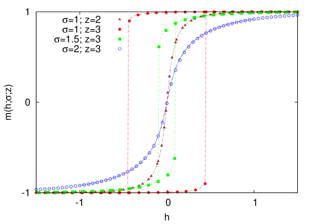
Figure 1: Hysteresis on directed random graphs of connectivity $z=2,3$ for a Gaussian distribution N(0,$\sigma^{2}$) of the random field. We have set $J=1$. Theoretical results are shown by continuous curves. Symbols depict results from numerical simulations of the model for a single configuration of the random-field distribution on a system of size $N=10^{6}$. Numerical results are indistinguishable from the theoretical results on the scale of the figure. Hysteresis is absent on a $z=2$ graph for any $\sigma$ and also on a $z=3$ graph if $\sigma>\sigma_{c}\approx 1.781$. For $\sigma<\sigma_{c}$ the loop has discontinuities at $h=\pm h_{c}$. The discontinuities reduce in size and move towards $h=0$ with increasing $\sigma$. As $\sigma\to\sigma_{c}$, the discontinuities vanish continuously at $h_{c}=0$.

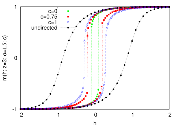
Figure 2: Hysteresis on a partially directed random graph with $z=3$ and $\sigma=1.5$ in units of $J$. A fraction $c$ of the nodes have two directed edges and one undirected. All three edges of the remaining fraction $1-c$ are undirected. Theoretical results are shown by continuous lines and simulations on a $N=10^{6}$ graph by symbols. Vertical portions of curves denote discontinuities. Results shown in Fig.1 are recovered for $c=0$. As $c\to 1$, the first-order jump in $m(h)$ reduces and moves away from the origin. A case where all three edges are undirected is also shown for comparison.

References

- (1) See for example, Spin Glasses and Random Fields, edited by A P Young ( World Scientific , 1997).
- (2) See for example The Science of Hysteresis edited by G Bertotti and I Mayergoyz (Academic Press, Amsterdam, 2006).
- (3) Y Imry and S-k Ma, Phys Rev Lett 35, 1399 (1975).
- (4) D Sherrington and S Kirkpatrick, Phys Rev Lett 35, 1792 (1975).
- (5) J J Hopfield, Proceedings of the National Academy of Sciences of the USA, vol. 79, no. 8, pp 2554-2558 (1982).
- (6) J Z Imbrie, Phys Rev Lett 53, 1747 (1984).
- (7) E Ising, Z Phys 31, 253 (1925).
- (8) L Onsager, Phys Rev 65, 117 (1944).
- (9) G H Wannier, Rev Mod Phys 17, 50 (1945).
- (10) I Syozi, Prog Theor Phys 6, 306 (1951).
- (11) G Parisi, J Phys A 13, L115-L121 (1980).
- (12) Spin Glass Theory and Beyond by M Mezard, G Parisi, and M Virasoro (World Scientific, 1987).
- (13) R J Glauber, J Math Phys 4, 294 (1963).
- (14) J P Sethna, K A Dahmen, S Kartha, J A Krumhansl, B W Roberts, and J D Shore, Phys Rev Lett 70, 3347 (1993).
- (15) D Dhar, P Shukla, and J P Sethna, J Phys A30, 5259 (1997).
- (16) J P Sethna, K A Dahmen, and C R Myers, Nature 410, 242 (2001), and references therein.
- (17) T P Handford, F J Peres-Reche, and S N Taraskin, Phys Rev E 87, 062122 (2013).
- (18) P Shukla and D Thongjaomayum, J Phys A: Math Theor 49, 235001 (2016); Phys Rev E 95, 042109(2017) and references therein.
- (19) M L Rosinberg, G Tarjus, and F J Perez-Reche, J Stat Mech: Theory Exp, P10004 (2008).
- (20) A Sirbu, V Loreto, V D P Servedio, and F Tria, arXiv:1605.06326v1.
- (21) W Quattrociocchi, G Caldarelli, and A Scala, Sci. Rep. 4, 4938 (2014).