Parameter estimation in modelling frequency response of coupled systems using a stepwise approach

Abstract

This paper studies the problem of parameter estimation in resonant, acoustic fluid-structure interaction problems over a wide frequency range. Problems with multiple resonances are known to be subjected to local minima, which represents a major challenge in the field of parameter identification. We propose a stepwise approach consisting in subdividing the frequency spectrum such that the solution to a low-frequency subproblem serves as the starting point for the immediately higher frequency range. In the current work, two different inversion frameworks are used. The first approach is a gradient-based deterministic procedure that seeks the model parameters by minimising a cost function in the least squares sense and the second approach is a Bayesian inversion framework. The latter provides a potential way to assess the validity of the least squares estimate. In addition, it presents several advantages by providing invaluable information on the uncertainty and correlation between the estimated parameters. The methodology is illustrated on synthetic measurements with known design variables and controlled noise levels. The model problem is deliberately kept simple to allow for extensive numerical experiments to be conducted in order to investigate the nature of the local minima in full spectrum analyses and to assess the potential of the proposed method to overcome these. Numerical experiments suggest that the proposed methods may present an efficient approach to find material parameters and their uncertainty estimates with acceptable accuracy.

1 Introduction

The scope of the current work is to investigate challenges arising in the solution of optimisation problems associated with the the performance of coupled dynamic systems or the estimation of their model parameters. Of particular interest is the occurrence of local minima, often posing a major obstacle in the solution of such problems.

There exist a vast amount of works published within the fields of material parameter estimation and optimisation. A comprehensive review of the literature is beyond the scope of the present paper; the interested reader is referred to [24, 16]. Most works discussing performance optimisation in structural-acoustic systems either work on the eigenfrequencies or limit the cost function to frequency bands containing a few resonances, see e.g. [28, 14, 29, 6, 1, 30, 13, 21].

However, the problem of interest here, i.e. estimation of model parameters in resonant, coupled problems over a frequency range containing a number of resonances, remains open. In particular those cases where, over the range of frequencies studied, there is a varying degree of interaction between the physical fields involved, are widely agreed to be subjected to local minima.

These often renders the parameter identification questionable if at all tractable, as demonstrated in previous works by the authors and others, see e.g. [23, 4, 15, 5, 20, 12]. The presence of resonances and anti-resonances in the spectrum is not the only factor responsible for local minima. In fact, it has been observed in previous works, see for example  [15, 5], that a sufficient degree of anisotropy is prone to induce such phenomena as well. The underlying cause for this is thought to be the self-similarity of the structural response at discrete combinations of the material, geometrical and loading properties. However, in order to distinguish between local minimas related to such dynamic response phenomena, and those related to the resonant spectrum fitting in itself, robust and efficient combinations of inversion methods are interesting to study.

The present paper addresses a method for overcoming local minima in the estimation of material properties in coupled dynamic resonant problems over a wide frequency band. The proposed approach relies on a stepwise solution, where the solution of each sub-problem is the starting point of the next. While a multi-step concept as such is not new, see for example [27] where a 3-step procedure was employed to enhance convergence,  [10] where different models are employed to fit sub-sets of parameters, and [19] where seismic waves are used to estimate subsurface properties using a frequency-by-frequency inversion approach, the proposed strategy is novel in that it specifically addresses resonant problems by employing an incremental frequency domain augmentation approach as discussed in the paper.

In our work, we have chosen to combine two different estimation methods, one based on a gradient, local search approach, [22], and one global search based on the Bayesian inversion framework, [24, 11, 2]. This enables us to combine the best of two analysis frameworks, [3, 20], complementing the deterministic search with additional insight into ill-posedness, measurement, and/or model uncertainties, etc. in the inverse problem. This adds a major advantage as the probability density computed from the Bayesian solution, reveals not only the different point estimates but also tells about the correlation between different parameters and also the credible intervals of the estimates. In addition, while the Monte Carlo based estimate converges to the global minimum if the number of samples is not limited, the combination provides more accurate initial conditions for the chain(s) and this holds the potential of reducing the computational time.

The proposed method is here demonstrated for a simplified one-dimensional fluid-structure problem exhibiting a complex behaviour, chosen for its computational tractability as well as being inexpensive to solve. The studied problem possesses a known solution and its fluid-structure coupling effects are limited to the interface between the two media. This provides the possibility to conduct extensive numerical experiments with controlled characteristics, such as frequency resolution, dissipative losses, nature of coupling, etc. The model problem chosen for the current work is selected based on the authors’ previous experiences from estimation in resonant systems involving soft materials, and the difficulties associated with local minima [5, 25, 26]. In the latter works, parameter estimation has required manual guidance to a certain extent in order for the cost function to converge. The authors aim herein at assessing the convergence behaviour of the proposed methodology, thus opening its applicability to more complex cases.

The paper is structured as follows. The model problem formulation is given next in Section 2. The deterministic and Bayesian inversion frameworks are introduced in Section 3 while Section 4 is dedicated to numerical experiments. Finally, discussion and conclusions are given in Sections 5 and 6, respectively.

2 Background and problem formulation

2.1 Model problem

Consider a freely moving one-dimensional (1D) solid body, excited at one end by a harmonic force of amplitude $F$, and coupled to an air cavity which is rigidly terminated at its other end, see Fig. 1. Both domains are modelled in the form of the 1D wave equation and have the same cross-section area $A$. Let $p$ denote the acoustic pressure in the air cavity, $u$ the linear solid displacement, $\rho_{s}$ the solid density, and $\rho_{f}$ the fluid density. The domain lengths are set to $L_{s}$ and $L_{f}$ for the solid and the fluid, respectively. The harmonic time dependence is chosen as $e^{+j\omega t}$, where $\omega$ is the angular frequency.

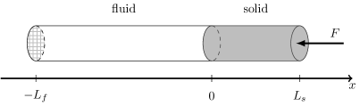
Figure 1: Schematic picture of the studied problem.

The solid and the fluid are both assumed to be damped, with loss factors $\eta_{s}$ and $\eta_{f}$, respectively. The complex speed of sound for the solid and the fluid may thus be written as

$$c_{s}^{2}=\hat{c}_{s}^{2}\left({1+j{\eta_{s}}}\right)\quad\mbox{and}\quad c_{f}^{2}=\hat{c}_{f}^{2}\left({1+j{\eta_{f}}}\right),$$ (1)

where $\hat{c}_{f,s}$ denotes the amplitude of the speeds of sound. The complex wave numbers for the fluid and solid are then

$$k_{f}=\frac{\omega}{c_{f}}\quad\mbox{and}\quad k_{s}=\frac{\omega}{c_{s}}.$$ (2)

The solution to the coupled problem is straightforward and will not be detailed here. The mean sound intensity level, at frequency $\omega$, radiated from the structure to the fluid is given by

$$I(\theta,\xi,\omega)=10\log\left(\frac{|\mathrm{Re}\left\{j\omega p_{0}u_{0}^{*}\right\}|}{2{I}_{\text{ref}}}\right),$$ (3)

where ${I}_{\text{ref}}=10^{-12}\,$W$\cdot$m^-2. The sound intensity level $I$ is used in the current work as the target quantity that the model should reproduce as a basis for the parameter estimation. In Eq. (3), the pressure and the solid displacement (at $x=0$) are given by

$$p_{0}=p_{0}\left(\theta,\xi,\omega\right) = \frac{F/A}{\cos\left(k_{s}L_{s}\right)-\dfrac{\rho_{s}c_{s}}{\rho_{f}c_{f}}\tan\left(k_{f}L_{f}\right)\sin\left(k_{s}L_{s}\right)},$$ (4)

$$u_{0}=u_{0}\left(\theta,\xi,\omega\right) = \frac{F/A}{\cos\left(k_{s}L_{s}\right)-\dfrac{\rho_{s}c_{s}}{\rho_{f}c_{f}}\tan\left(k_{f}L_{f}\right)\sin\left(k_{s}L_{s}\right)}\frac{\tan\left(k_{f}L_{f}\right)}{\rho_{f}c_{f}\omega}.$$ (5)

In Eqs. (3-5), $\xi$ denotes the set of known parameters and $\theta$ the set of unknown parameters,

$$\xi = \left\{\rho_{f},\rho_{s},L_{f},L_{s},A,F\right\},$$ (6)

$$\theta = \left\{\hat{c}_{f},\hat{c}_{s},\eta_{f},\eta_{s}\right\}.$$ (7)

2.2 Target properties

As stated in the introduction, the problem chosen is selected on the basis of it being simple to model and having a low computational cost, yet complex enough to exhibit local minima, which pose a formidable challenge to most approaches for inverse modelling. The fixed parameters for the solid have been chosen to be representative of a fairly light open-cell polymer foam, with a density low enough to induce a strong coupling with the air cavity over a wide frequency range.

The parameters for the target model are shown in Table 1, where $\theta^{\text{meas}}$ denotes the target parameters governing the measured system.

Table 1: Fixed parameters $\xi$ and target parameters $\theta$ for the studied problem.

	Fluid		Solid		Global
$\xi$	$\rho_{f}$ $(\mbox{kg/m}^{3})$	$L_{f}$ (m)	$\rho_{s}$ $(\mbox{kg/m}^{3})$	$L_{s}$ (m)	$F$ (N)	$A$ $(\mbox{m}^{2})$
	1.2	1	30	0.338	1	0.01
$\theta^{\text{meas}}$	$\hat{c}_{f}$ (m/s)	$\hat{c}_{s}$ (m/s)	$\eta_{f}$	$\eta_{s}$	-	-
	343.5	57.735	0.0005	0.0005

With the chosen target model parameters, the fundamental frequencies and first harmonics of the uncoupled resonances of the fluid and the solid are shown in Table 2. Note that the fundamental frequencies of the two systems are well separated, and hence implying a moderately strong interaction between the fluid and the structure for these. Also, the fundamental resonance of the fluid cavity is within 1 Hz from the first harmonic of the solid, which leads to the well-known up- and down-ward shifts in the coupled frequencies occurring for every second resonance of the solid, as will be shown below.

Table 2: Fundamental $f^{0}_{f,s}$ and first harmonics $f^{1}_{f,s}$ of the uncoupled resonances of the fluid and the solid.

$f_{f}^{0}$ (Hz)	$f_{f}^{1}$ (Hz)	$f_{s}^{0}$ (Hz)	$f_{s}^{1}$ (Hz)
171.75	343.5	85.35	170.7

As the focus is here on the phenomena rather than computation efficiency, a frequency range of $0.5-1000\,$Hz is used, with a frequency resolution of $0.0153\,$Hz, in the numerical experiments performed.

3 Inverse problem

3.1 Observation model

Recalling the aim of this work, together with the choice of model problem as described above, we consider also the influence of noise in the target spectrum data, from now on referred to as measurement data. This choice is partially made in order to avoid the ”inverse crime” trap discussed below, but also to render the measurement data set more realistic and in this way obtain a preliminary assessment of the robustness of the proposed method. For the purpose of the current work, the noise is introduced in the form of additive errors on the sound intensity. The observation model may thus be written as

$${I}^{\text{meas}}\left(\theta,\xi,\omega^{(\nu)}\right)={I}\left(\theta,\xi,\omega^{(\nu)}\right)+e,$$ (8)

where $\omega^{(\nu)}\in{\mathbb{R}}^{N_{f}\times 1}$ ($N_{f}$ denotes the number of frequencies) and $e$ models the measurement error. In this work, error $e$ is assumed to be Gaussian distributed with zero mean and covariance $\Gamma_{e}=\sigma_{e}^{2}I$, that is $e\sim\mathcal{N}\left(0,\Gamma_{e}\right)$. In the covariance matrix, $\sigma_{e}$ denotes the standard deviation of the noise and $I$ is the $N_{f}\times N_{f}$ identity matrix.

As stated in the introduction, we have chosen to apply and combine two different approaches to the inverse problem, a gradient search method and a method based on a Bayesian framework. Both of these are well-known and have been discussed in numerous papers, thus we will not go into details about either of them as the focus here is on the estimation and the problem of local minima in resonant systems.

Each method is run several times in order to get some statistics of their respective convergences to the target model. For each such repeated computation, the starting point is generated from a uniform distribution between the lower and the upper bounds of each of the variables respectively.

3.2 Numerical target

In the current work, a purely simulation-based generation of the measurement data is used and these are fitted with an analytical model. In such studies, it is of great importance to avoid committing an ”inverse crime” [11]. Our choice for avoiding this is to use a discretized solution, leading to a different numerical accuracy for generating simulated measured data and the model fitted in the inversion. In this paper, we thus generate the measured data set using the Comsol Multiphysics software version 5.3a while in the inversion we use the analytic solution of the problem.

For the Comsol model, which consist of an axi-symmetric model, the element size is $L^{e}_{r}=L^{e}_{x}=0.0058\,$m for the solid elements in a mapped quadrilateral mesh with second order shape functions, while for the fluid we choose elements with $L^{e}_{x}=0.0344\,$m and $L^{e}_{r}=0.0058\,$m. Thus the mesh is compatible along the interface between the fluid and the solid. For both media these element lengths observe $L^{e}_{x,r}<\lambda_{\min}/10$ for $\lambda_{\min}=c_{s}/f_{\max}$.

With increasing frequency, the relative quadratic error between the discretized Comsol and the analytical solutions grows to around 7%, as shown in Fig. 2.

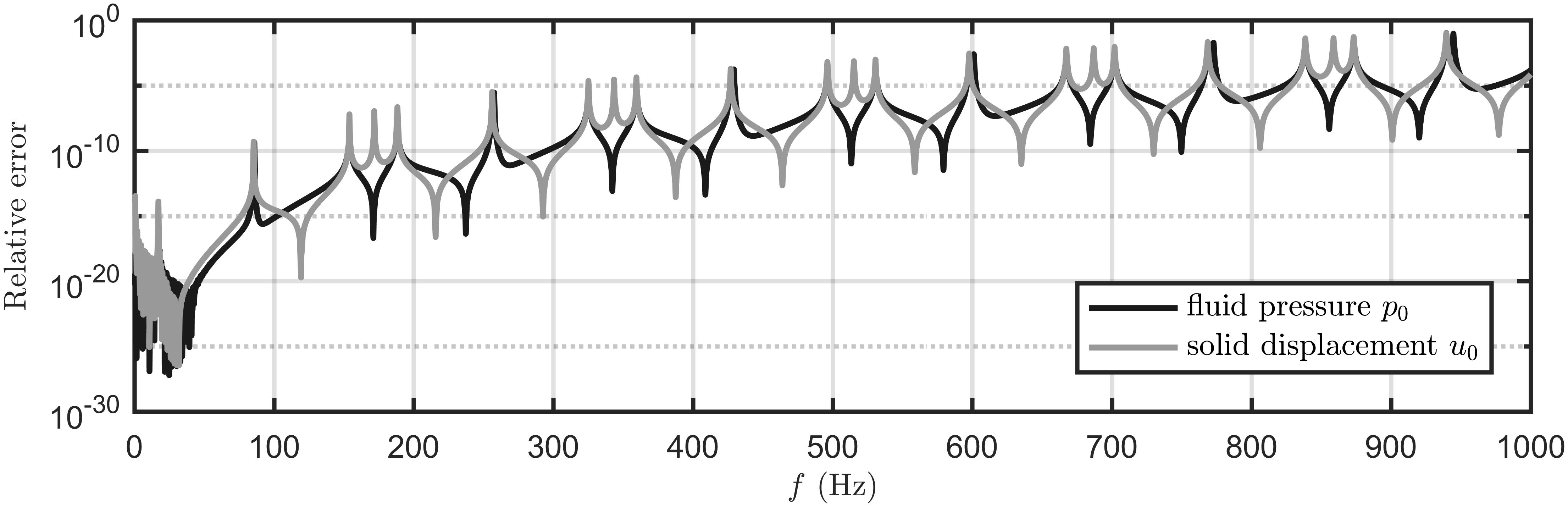
Figure 2: Relative quadratic error for the coupled Comsol and analytical solutions, pressure in fluid domain and displacement in solid.

3.3 Deterministic framework

For the gradient search, the Globally Convergent Method of Moving Asymptotes (GCMMA) is used in the current work [22]. The cost function to be minimised is defined as

$$K(\theta)=\sum_{\ell=1}^{N_{f}}\frac{\left|{I}^{\text{meas}}\left(\theta^{\text{meas}},\xi,\omega^{(\nu)}_{\ell}\right)-I\left(\theta,\xi,\omega^{(\nu)}_{\ell}\right)\right|^{2}}{\left|{I}^{\text{meas}}\left(\theta^{\text{meas}},\xi,\omega^{(\nu)}_{\ell}\right)\right|^{2}},$$ (9)

where $\theta\in\mathcal{A}$, with $\mathcal{A}=\left[\theta_{\min},\ \theta_{\max}\right]$. The parameters $\theta$ are not subjected to any additional constraints. We employ a re-scaling of all design variables such that they are mapped to the dimensionless domain $\theta\in[1,2]$, see [4] for more details. The gradients required for the cost function are computed using finite differencing, with a step of $d\theta=10^{-12}$.

In the analysis, a termination criterion of the GCMMA iterations is set to $10^{-8}$ for the variation of the cost function and $10^{-6}$ for the change in the design variables, as monitored over 5 subsequent iterations. As the focus is on the problem of local minima, and not on computational efficiency, the number of iterations for each gradient solution is allowed to reach 600 in order to ensure that the iterations are terminated based on convergence, to facilitate the evaluations described below.

In the following, the solutions obtained from the gradient search method will be referred to as GCMMA.

3.4 Bayesian framework

In the Bayesian framework [24, 11, 2], estimated variables $\theta$ are modelled as random variables. In this inference, the main tasks are to construct the likelihood and prior models $\pi({I}^{\text{meas}}\,|\,\theta)$ and $\pi(\theta)$, respectively. The likelihood model gives the relative probabilities that the model generates the observations ${I}^{\text{meas}}$ over all choices of parameters, while the prior model sets constraints on the model parameters. The solution to the inverse problem in the Bayesian framework is coded in the posterior distribution $\pi(\theta\,|\,{I}^{\text{meas}})$, which gives the relative probability of the unknowns $\theta$ given the observations ${I}^{\text{meas}}$. The posterior distribution is obtained by Bayes’ formula

$$\pi\left(\theta\,|\,{I}^{\text{meas}}\right)\propto\pi\left({I}^{\text{meas}}\,|\,\theta\right)\pi(\theta).$$ (10)

The additive observation model (8) allows us to write the likelihood model as follows

$$\pi({I}^{\text{meas}}\,|\,\theta)=\pi_{e}\left({I}^{\text{meas}}-{I}\left(\theta,\xi,\omega^{(\nu)}\right)\right),$$ (11)

where $\pi_{e}$ is the probability density of the error $e$. Since the error $e$ is assumed to be Gaussian, the likelihood density can be written as

$$\pi({I}^{\text{meas}}\,|\,\theta)\propto\exp\left\{-\frac{1}{2}\bigg{(}{I}^{\text{meas}}-{I}\left(\theta,\xi,\omega^{(\nu)}\right)\bigg{)}^{\top}\Gamma_{e}^{-1}\bigg{(}{I}^{\text{meas}}-{I}\left(\theta,\xi,\omega^{(\nu)}\right)\bigg{)}\right\}.$$ (12)

Furthermore, we use uniform prior of the form:

$$\pi(\theta)\propto\begin{cases}{}1&\text{if }\theta\in\mathcal{A}\\ 0&\text{otherwise.}\end{cases}$$ (13)

For the sampling of the posterior densities, we use the Metropolis-Hastings algorithm [18, 17, 9] with an adaptive proposal distribution scheme [7, 8]. The adaptive algorithm automatically adjusts the spatial orientation and size of the proposal density considering all of the target distribution points accumulated so far, leading to a faster convergence.

As an initial condition for the Markov chain, we use either the GCMMA solution or random starting point and run it for 1,030,000 iterations including a burn-in of 30,000 (unless stated otherwise in the text). From the burn-in, the last 20,000 samples are used to provide an initial estimate of the covariance matrix for the adaptive proposal distribution scheme. As the proposal density, in the first 30,000 samples, we use a zero mean Gaussian distribution, in which parameters are assumed to be uncorrelated.

The point estimate for the parameters we use in this work is the maximum a posteriori (MAP) which corresponds to the point in the posterior density that has the highest probability. As an indication of the uncertainty in the point estimates we use the (narrowest) 95% credible interval, which represents the spread of the posterior density. In the following, the solutions obtained from the Bayesian inversion will be referred to as MCMC (Markov chain Monte Carlo).

4 Numerical experiments

This section presents the results obtained for the local minima problems in focus here. First the inverse problem for the whole frequency range is solved, this will be referred to as the full spectrum estimation, including an analysis of the character of the local minima as such. The proposed stepwise method is then introduced as a means to overcome these problems.

In the following examples, estimated parameters are restricted to the interval, $\eta_{s}\in\ ]0,\ 1],\eta_{f}\in\ ]0,\ 1],\ c_{f}\in\ [10,\ 700]\ \mbox{m/s}$, and $c_{s}\in\ [10,\ 700]\ \mbox{m/s}$ which is referred to as the prior model in the Bayesian framework. This choice is made in order to avoid adding a priori knowledge with respect to each of the coupled sub-systems while still keeping a reasonable range of possible parameter values.

4.1 Full spectrum estimations

In order to explore the nature of possible local minima resulting from GCMMA, we attempted an estimation of the parameters given in Table 1, for a noise-free target spectrum generated through a Comsol simulation as described above.

Figure 3 shows the initial and final parameter values for 392 different full spectrum estimations using random starting points, none of which converged to the global minimum. The speed of sound for the fluid tends to be close to the target value for most of the solutions, while the speed of sound for the solid seems to converge towards values that are considerably higher than the target value.

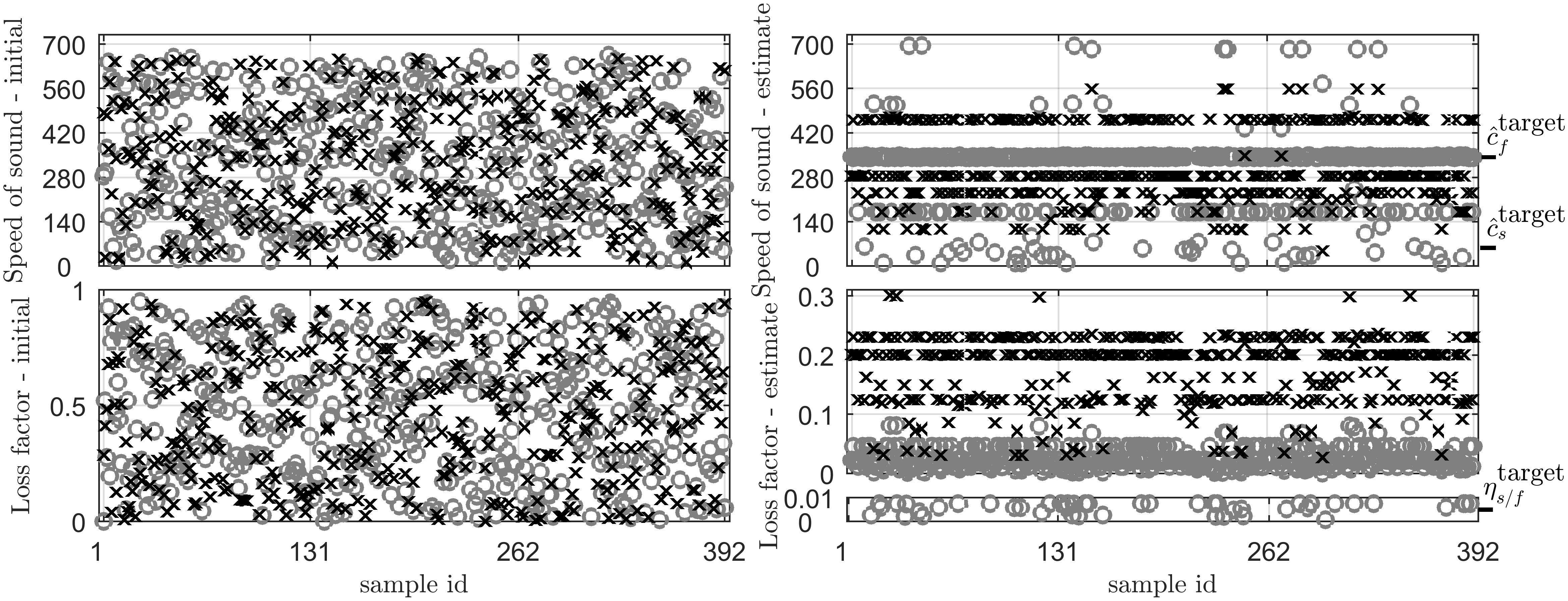
Figure 3: Left: Random starting points for full spectrum solution. Right: Resulting design variables, including a close-up on the $[0,\ 0.01]$ interval of the y-axis for the bottom right sub-figure. The solid parameters are denoted by “$\times$” and the fluid by “${\color[rgb]{.5,.5,.5}\circ}$”.

These results illustrate the well-known difficulties encountered when fitting a parametric model over a wide range of frequencies, containing a large number of coupled resonances. In fact, in order to identify the parameters in Table 1 on the full spectrum, the initial values for $\theta$ must lie in the close neighbourhood of the target values.

4.2 Investigating the local minima

In this section, the focus is on two randomly chosen samples from Fig. 3, with the intention to study the results from the full spectrum estimations in more detail. We have selected starting points that are fairly close to the target value for the fluid speed of sound, but far away from the solid, the first having close to 10 times higher and the second nearly half the target value. Thus, the points

$$\theta_{1}^{\text{init}} =[311.7367,507.3036,0.0001,0.3023],$$

$$\theta_{2}^{\text{init}} =[324.3726,28.8632,0.5497,0.4353],$$

yield the following local minima,

$$\theta_{1}^{\text{full}} =[344.9533,284.8150,0.0221,0.2007],$$

$$\theta_{2}^{\text{full}} =[342.8467,462.1551,0.0458,0.2304].$$

The results are shown in Fig. 4 in terms of sound intensity level. For both $\theta_{1}$ and $\theta_{2}$, $\hat{c}_{f}$ is close to the value used in the target model, while for neither of the two design points $\hat{c}_{s}$ is close to the target model value. In addition, as observed in the close-up $y\in[0,\ 0.01]$ in Fig. 3, none of the estimates for the solid loss factor have converged to the target value, see Table 1.

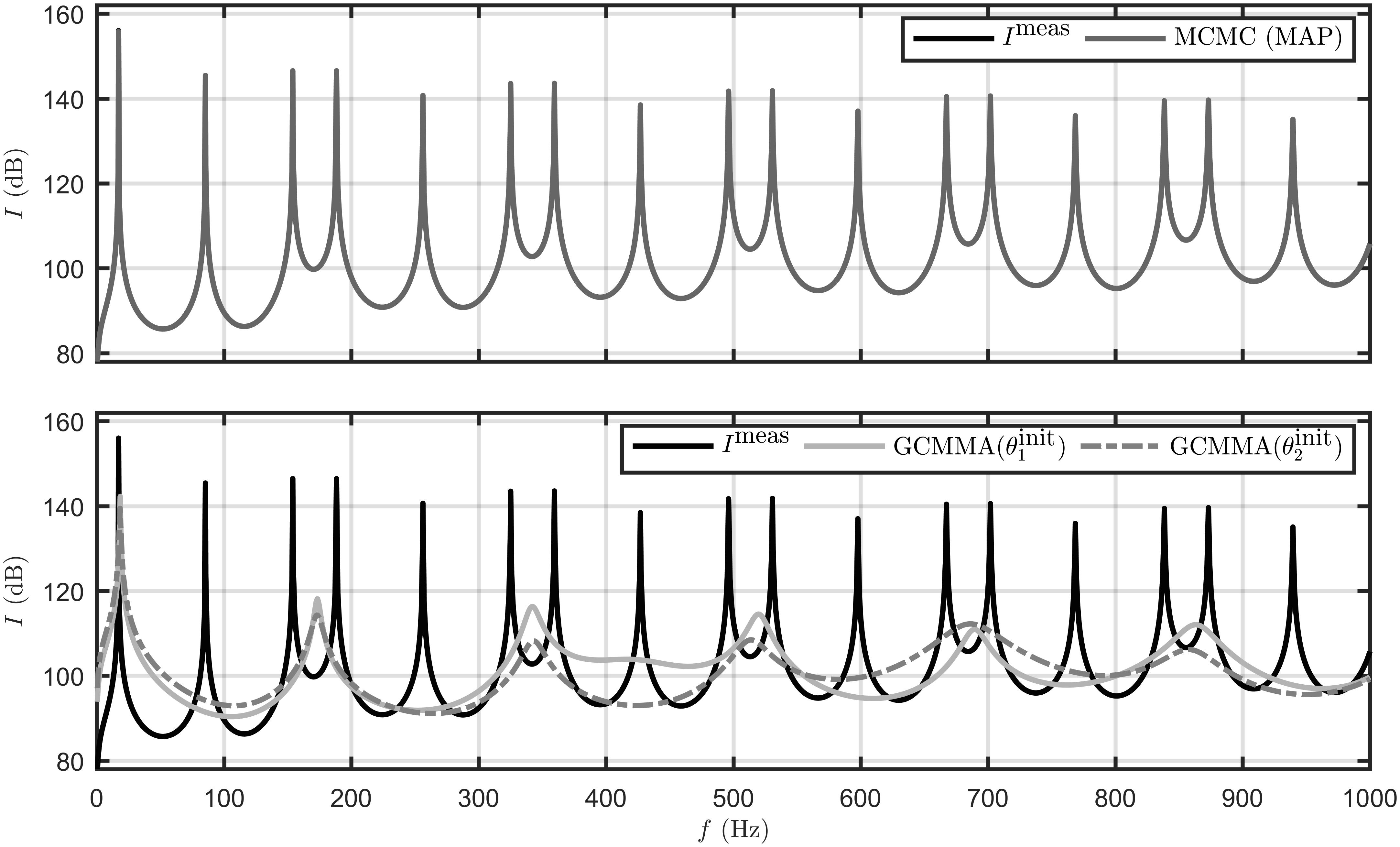
Figure 4: Fit of noise-free measurements. Top: The MCMC based MAP estimate after 2,000,000 samples, without use of adaptive proposal distribution scheme. Bottom: gradient based solutions $\theta^{\text{full}}_{1}$ and $\theta^{\text{full}}_{2}$ (using initial points $\theta^{\text{init}}_{1}$ and $\theta^{\text{init}}_{2}$).

The solutions obtained are quite typical for the two different inversion approaches. With the restrictions set, primarily in terms of number of iterations, GCMMA terminates at different local minima which clearly are far from the true solution, while MCMC identifies the target model but often needs a long chain to find the global minimum. Note that in Fig. 4, the MCMC solver does not use adaptivity. For the purpose of this investigation of the local minima, the proposal density is assumed to be wide, allowing the chain to jump between different local minima more easily.

In order to confirm whether the obtained GCMMA solutions correspond to local minima of Eq. (9), the vicinity of $\theta_{1}^{\text{full}}$ and $\theta_{2}^{\text{full}}$ is explored using MCMC. Here, the MCMC algorithm uses the adaptive proposal density after the 30,000 initial rounds but it is assumed that the proposal density in these initial rounds is narrow in order to restrict $\theta$ to the neighbourhood of these GCMMA solutions. Figures 5 and 6 show that both solutions obtained are indeed local minima. All four design variables influence the cost function to the same extent and obviously there is no direction in which a gradient search can expect a lowering of the cost function further. In addition, it can be observed from these two figures that the correlation between the model parameters vary between almost totally uncorrelated (see e.g. in Fig. 5 $\hat{c}_{f}$ and $\hat{c}_{s}$) and higher correlation (e.g. $\hat{c}_{f}$ and $\eta_{f}$; $\eta_{f}$ and $\eta_{s}$). Furthermore, the 95% credible intervals reveal that the local minima are indeed narrow in all parameters.

It is worthwhile to explore the solutions obtained for the full spectrum in some more detail. In almost all cases we have observed, the first resonance in the response spectrum (see Fig. 4) is well identified with respect to the frequency but not particularly well in terms of amplitude. The gradient solutions appear in many cases to track the uncoupled resonances, see for example the peak in the GCMMA solutions in Fig. 4 which occurs at about 172.4 Hz and the peak at 342.2 Hz, both very close to the uncoupled fluid resonance frequencies given in Table 2. In most of the solutions, this appears to be achieved through converging towards design points where, e.g. $\hat{c}_{f}\approx\hat{c}_{f}^{\text{target}}/2$ or $\hat{c}_{f}\approx\hat{c}_{f}^{\text{target}}$; and $\hat{c}_{s}\approx 2,4,5,8\times\hat{c}_{s}^{\text{target}}$, see Fig. 3. An interpretation of these solutions is that they tend to combine resonances in one of the uncoupled systems with anti-resonances in the other. Together with associated high loss factors this leads to the fitting to the anti-resonant parts of the target spectrum that may be observed in the lower part of Fig. 4.

As a concluding remark of this subsection, similar findings have been observed for a case with target loss factors of 10%, and these will not be repeated here for the sake of conciseness.

Figure 5: Two-dimensional (2D) marginal densities for the $\theta_{1}$. The cross denotes the maximum a posteriori estimate (MAP) and triangle is the initial condition $\theta_{1}$. Here the proposal density in the burn-in phase of the MCMC is assumed to be narrow in order to restrain estimated parameters to the neighbourhood of the GCMMA-based point estimate. The dots represent a sample of the MCMC points and $r$ is the Pearson correlation coefficient. The black curves on the bottom and left side of each plot are the 1D marginal posterior densities. For the 1D densities, the light gray zone denotes the narrowest 95% credible interval (bounds given in the figure).

Figure 6: 2D Marginal densities for the $\theta_{2}$, otherwise same caption as in Fig. 5.

4.3 Stepwise approach

A major point of attractiveness of GCMMA for solving inverse problems is its low number of model evaluations [22]. However, as illustrated above, a pattern of local minima hinders the unsupervised determination of the global minimum or the full spectrum problem. Observations made when studying full spectrum solutions such as those in Sec. 4.1 triggered the idea for the stepwise approach presented here for solving inverse problems involving frequency-dependent experimental data exhibiting a resonant behaviour. The method draws on the observations made related to the correlation between the model parameters as well as the convergence of the gradient method with respect to the lowest resonances of the coupled system. The concept is simple, yet, as detailed in what follows, remarkably powerful and robust.

The first step of the method consists in defining a number of sub-problems in which the problem is solved within a frequency interval from the lowest available frequency to an incrementally higher frequency limit, i.e.

$$F_{\ell}^{\text{sub}}=\left[f_{\min},\ f_{\max}^{(\ell)}\right],\quad\ell=1,\ldots,{N^{\text{sub}}}.$$ (14)

In the very first step, i.e. when solving for $F_{1}^{\text{sub}}$, $\theta^{\text{init}}$ is randomised such that $\hat{c}_{s}$ and $\hat{c}_{f}$ are sampled with equal probability from the interval $[10,\ 700]$ m/s and damping factors $\eta_{s}$ and $\eta_{f}$ from the interval $]0,\ 1]$, i.e. the prior model. In each of the subsequent $\ell$-th steps, $\theta_{\ell}^{\text{init}}$ holds the parameters estimated from the solution obtained in the previous step, i.e. $\theta_{\ell}^{\text{init}}=\theta_{\ell-1}$. That is, the point estimate obtained from the first subdivision is used as a starting point for the next frequency interval until the entire available spectrum is covered. The last step corresponds to an estimation in the full spectrum $F_{N^{\text{sub}}}^{\text{sub}}$ where the starting point has been guided by the sequence of previous steps.

4.4 Application to the simplified fluid-structure interaction problem

This subsection presents the application of the proposed stepwise approach to estimating the parameters of the target model given in Table 1. The focus is on the convergence of the method and therefore the computational efficiency aspects are not discussed at this point.

The application of the proposed approach to the dataset shown in Fig. 4 yields systematically satisfactory results, only limited by the numerical stopping criteria set for the optimiser. As these results do not convey a significant deal of information, the performance and robustness of the method are presented on a dataset containing additive noise. This is done in order to demonstrate how the stepwise approach performs for a more realistic set of data, by including a standard deviation $\sigma_{e}=2\,$dB SIL (where SIL stands for sound intensity level) assumed for the zero mean white noise model $e$ in Eq. (8).

In setting up the estimation problem, the frequency spectrum $f\in[0.5,\ 1000]\,$Hz is divided into $N^{\text{sub}}=5$ frequency intervals, having maximum frequencies $f_{\max}=\{5,\ 25,\ 75,\ 150,\ 1000\}\,$Hz, see Eq. (14). This choice, which obviously is far from unique, is based on the observations made in Sec. 4.2 on the lowest peak in the response occurring at circa 17.5 Hz and the correlations between $\hat{c}_{f}$ and $\hat{c}_{s}$. In particular, the first substep is aimed at capturing the low frequency asymptotic behaviour and the parameters governing this, in this case $\hat{c}_{f}$ and $\eta_{f}$ as will be discussed later.

Using $\theta^{\text{init}}=\theta_{2}^{\text{init}}$, given in Sec. 4.2, as a starting point, the results in Fig. 7 are obtained. The fit between the target and the estimated model is very close, and for comparison, the less satisfactory estimation results when using the full spectrum for the inversion are also shown.

Figure 7: $I$ as a function of frequency: model including additive noise, final step in the proposed approach, and full spectrum estimates following Table 3.

The convergence history for the stepwise solution is shown in Table 3, together with the full spectrum estimates and initial and target parameters. The stepwise solution and the target values are also visualized in Fig. 8. Interestingly the path to the target solution is by first finding the loss factor for the fluid while the loss factor for the solid goes to the maximum allowed. By the third step, all remaining parameters have been estimated. Note that this is achieved for a quite noisy target dataset.

Table 3: Table lists the starting point $\theta^{\text{init}}$, estimates for different frequency intervals of the stepwise approach, estimate for the full spectrum, and target values.

	$\theta$	$f_{\max}\,$(Hz)	$\hat{c}_{f}\,$(m/s)	$\hat{c}_{s}\,$(m/s)	$\eta_{f}\times 1000$	$\eta_{s}\times 1000$
Starting point	$\theta^{\text{init}}$	-	$324.3726$	$28.8632$	$549.6625$	$435.3224$
Stepwise approach	$\theta_{1}^{\text{step}}$	5	$308.9829$	$218.6860$	$0.3969$	$454.5294$
	$\theta_{2}^{\text{step}}$	25	$321.0744$	$230.1108$	$0.4735$	$450.6748$
	$\theta_{3}^{\text{step}}$	75	$343.3354$	$57.8623$	$0.4985$	$0.0099$
	$\theta_{4}^{\text{step}}$	150	$343.4514$	$57.7347$	$0.4956$	$0.4701$
	$\theta_{5}^{\text{step}}$	1000	$343.5040$	$57.7375$	$0.4997$	$0.4999$
Full spectrum	$\theta^{\text{full}}$	1000	$342.8564$	$460.7882$	$45.7421$	$230.8025$
Target	$\theta^{\text{meas}}$	1000	$343.5000$	$57.7350$	$0.5000$	$0.5000$

Figure 8: Resulting estimates after each of the incremental frequency intervals of the stepwise approach, same data as in Table 3. Horizontal black lines show the target parameter values.

In analysing the convergence behaviour of the stepwise approach, it should be kept in mind that in each substep the subproblems solved are different from the full spectrum problem. Nevertheless, the solutions to the incremental steps provide a path of incremental partial global minima towards the global minimum of the full spectrum problem.

4.5 Marginal densities for the different steps

Figures 9, 10, and 11 show the marginal densities at the end of steps $f\leq 5\,$Hz, $f\leq 75\,$Hz, and $f\leq 1000\,$Hz. The estimates found at the end of the first step, Fig. 9, indicate that there is a strong correlation between the fluid loss factor and the fluid speed of sound, but the remaining parameters are neither correlated to each other nor influencing the solution to the subproblem as such.

At the 3th step, the correlation is strong between $\hat{c}_{s}$ and $\hat{c}_{f}$, and it can be observed that both have indeed converged to the target values. As the full spectrum is solved in the final step, all parameters have been estimated within 5% relative error, with the largest deviations occurring in the loss factors, in this case related to the noise in the measured data set used for the estimation. The figures also show how the credible interval becomes narrower when the amount of data is increased for all parameters. The true value is found within the narrowest 95% credible intervals in all other cases, except in Fig. 11 for $\hat{c}_{s}$ but also here the distance between the point estimate and the true value is acceptable, given the uncertainties in the measurement data.

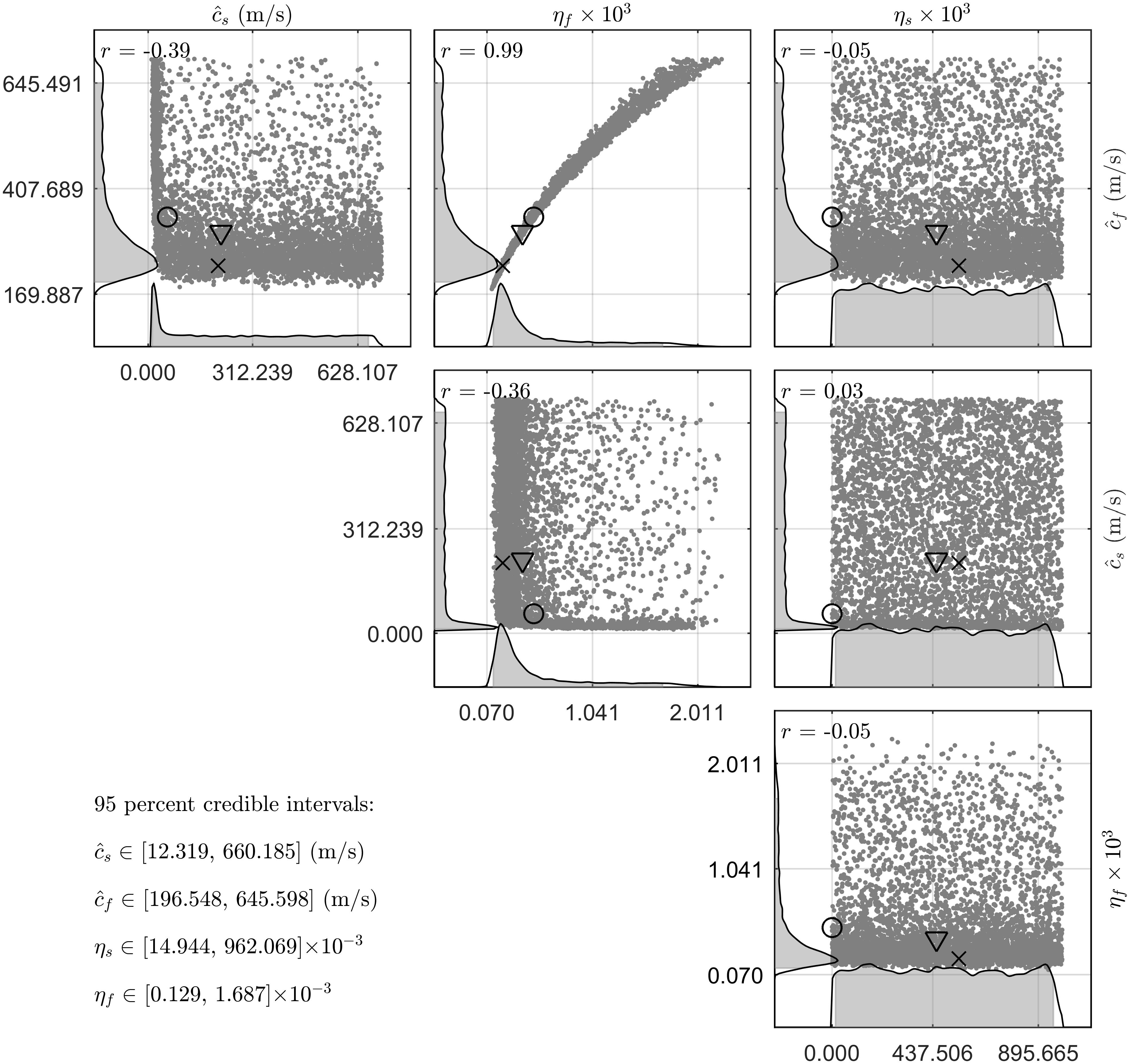
Figure 9: 2D Marginal densities for the substep $f\leq\,$5 Hz data. The cross denotes the maximum a posteriori estimate (MAP), the triangle is the initial condition (based on GCMMA estimation, Fig. 7), and the circle is the true value. The dots represent a sample of the MCMC points and $r$ is the Pearson correlation coefficient. The black curves on the bottom and left side of each plot are the 1D marginal posterior densities. For the 1D densities, the light gray zone denotes the narrowest 95% credible interval (bounds are given in the figure).

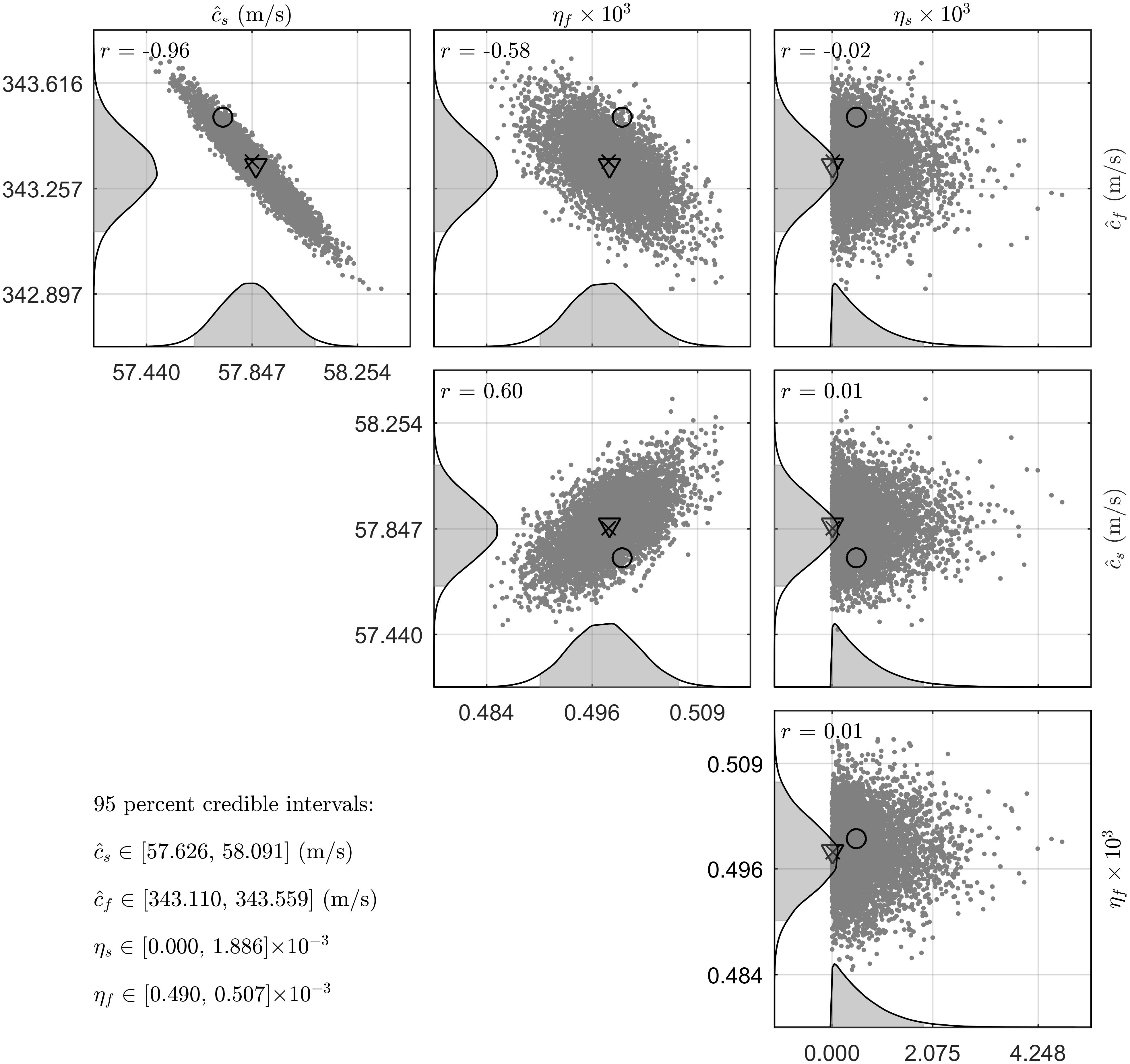
Figure 10: Results for the the substep $f\leq 75$ Hz, otherwise same caption as in Fig. 9.

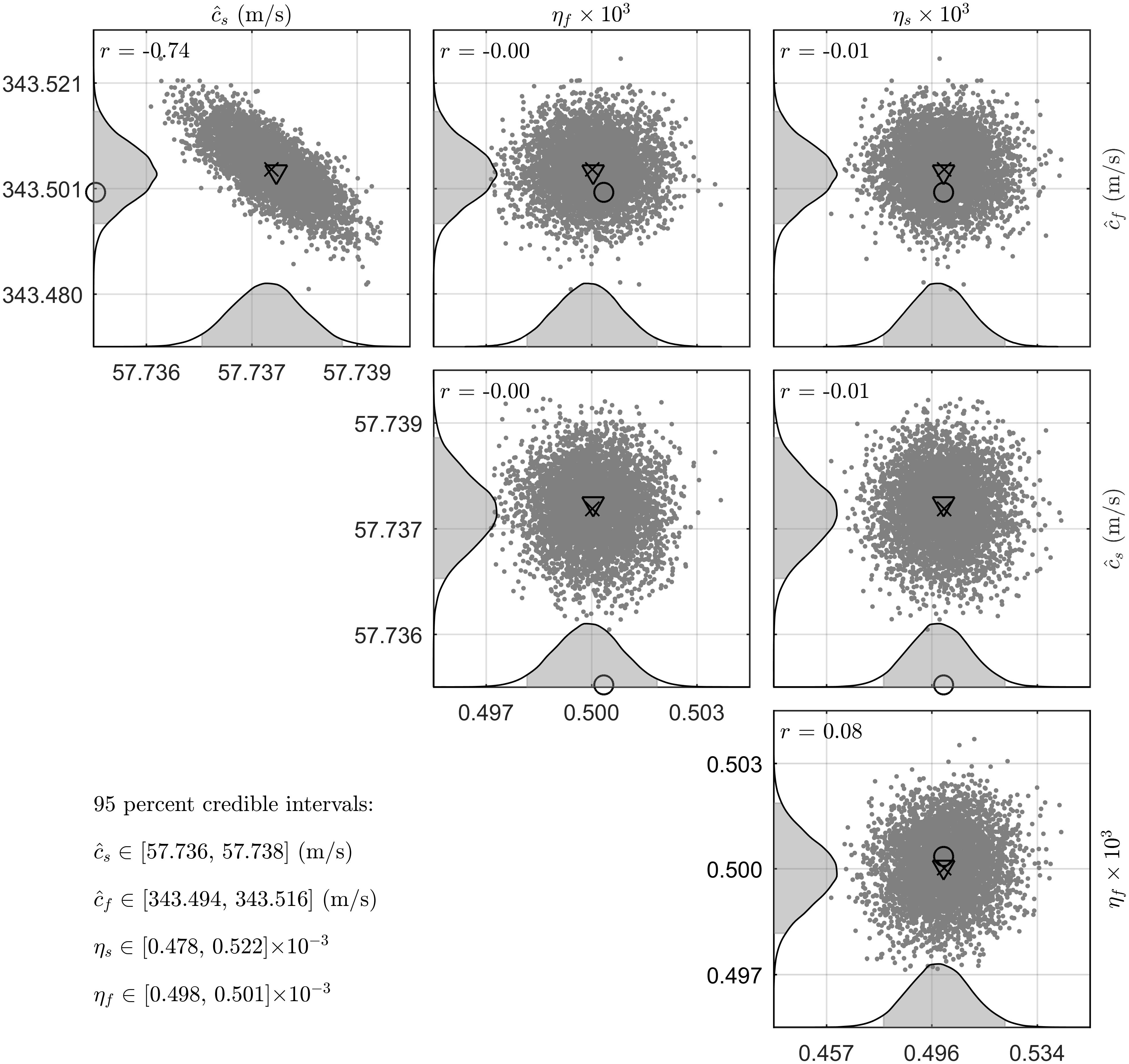
Figure 11: Results for the last substep $f\leq 1000$ Hz, otherwise same caption as in Fig. 9.

To study the robustness of the stepwise approach when applied to the model problem studied in the current work, we performed 392 runs, using the same randomly chosen starting points as in Fig. 3. Out of these 9 did not converge to the global minimum, see Fig. 12. In the converged solutions, the speeds of sound for both fluid and solid, as well as the loss factor for the fluid are estimated within 1% relative prediction error, while in particular the loss factor for the solid is less accurately estimated. The largest discrepancy observed for the latter is about 15%.

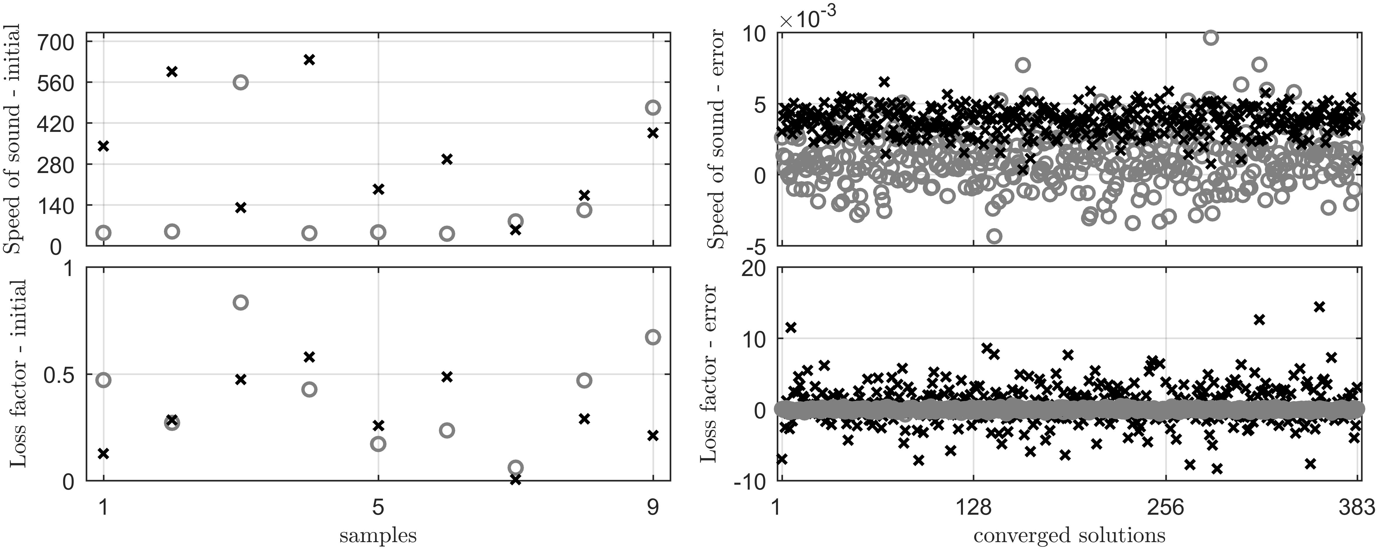
Figure 12: Left: Sample starting points that did not converge. Right: Relative prediction error for the converged samples. The solid parameters are denoted by “$\times$” and the fluid by “${\color[rgb]{.5,.5,.5}\circ}$”.

5 Discussion

As mentioned above, the success of the proposed stepwise approach appears to be linked to the dominant model parameters and the correlations between these and their variations over the different parts of the frequency spectrum studied. This is in agreement with the findings in [27, 10].

In fact the correlation between parameters observed above for the current model problem, may be illustrated further by taking the limit for the Helmholtz numbers $k_{f}L_{f},k_{s}L_{s}\ll 1$, of Eq. (8). This may be shown to be

$$I(\theta,\xi,\omega)\approx\frac{{{{\left({F/A}\right)}^{2}}}}{{\dfrac{{{\rho_{f}}\hat{c}_{f}^{2}}}{L_{f}}}}\dfrac{{\omega\eta_{f}}}{{1-\dfrac{{{\omega^{2}}}}{{\dfrac{{{\rho_{s}}\hat{c}_{s}^{2}}}{L_{s}}}}\left({{\rho_{s}}{L_{s}}+2{\rho_{f}}{L_{f}}}\right)}},\quad{\eta_{f}},{\eta_{s}}\ll 1.$$ (15)

Accordingly, as observed above, for the first substep in the solution of the current model problem, $\hat{c}_{f}$ and $\eta_{f}$ are the two model parameters that control the behaviour of $I$ in Eq. (3). This in itself motivates our choice of the first sub-divisions in the previous section, and in particular the choice of the frequency range for the first substep, which in many of the converged solutions is critical for the success. By restricting the first substep solution to essentially fitting Eq. (15) to the target spectrum, the ratio between the fluid loss factor and the square of the fluid speed of sound, which according to Eq. (15) is governing the intensity at low frequencies, is obtained, i.e. $\sim 4.237610^{-09}$, already at the end of the first step as  $\sim 4.157310^{-09}$. As a matter of fact such ratio is invariant along the path in the marginal density for $\hat{c}_{f}$ vs. $\eta_{f}$, Fig. 9.

A crucial aspect for the interpretation of the solution to the first step is the fact that the marginal densities related to the solid loss factor are nearly uniform. This indicates that the cost function is not sensitive to this parameter for the first step, which in turn suggests that the sound intensity radiated by the solid into the air cavity does not strongly depend on $\eta_{s}$ at very low frequencies, as confirmed by Eq. (15).

In addition, Eq. (15) and Fig. 9 suggest that the low-frequency asymptotic behaviour of the system becomes increasingly sensitive to decreasing values of the speeds of sound. This translates into the difficulty for a gradient-based optimiser to approach the correct solution from substantially low values of the speeds of sound.

As identified in the convergence of repeated runs from random starting conditions, Fig. 12, the estimates related to the solid loss factors are the least accurate. We relate this to the numerical model in Comsol, used as measurement data, and the computational errors associated with it, see Fig. 2 where it is shown that the solid displacement is the dominating source of error for most frequencies in the spectrum. Together with the added noise, this renders the convergence in the final substep mostly to be controlled by the solid loss factor, see for example Table 3 and Fig. 11.

The choice of the lower bounds of the parameter range used, in particular for the speeds of sound, was dictated by our observations when studying the full spectrum convergence behaviours. In fact, the robustness of the approach relies on the ability of the first step to fit the asymptotic behaviour. Lower speeds of sound would accordingly require a lower high-frequency limit for the first step.

Although its general applicability is still to be confirmed by exploring real parameter estimation cases, the significant improvement in convergence experienced for the current coupled fluid-structure problem is indisputable in our opinion. We ran almost 400 analyses with uniformly distributed random initial starting points, all but a few converged to the target solution.

Even though the focus of the current work is not on computational efficiency, it is worth noting that as the frequency range of the first steps is relatively narrow, it is far less expensive to compute the cost function for these as compared to the full spectrum approach. Thus, it should be beneficial to allow for a higher number of iterations, i.e. employing more stringent convergence criteria in the first increments of the stepwise estimation, in order to reduce the efforts required in the last steps. This is obviously a trade-off that most likely is problem-dependent as well as depending on the starting point and the path required to reach the global minimum.

6 Conclusions

Solving estimation problems over a wide frequency range with several resonances is difficult due to local minima, which arise due to partial fits to the spectrum. Such an obstacle is particularly severe for gradient search methods. Nonetheless, also global search approaches face difficulties, requiring a large number of iterations.

In the present paper, the proposed stepwise inversion approach is run using several hundreds of random starting points in the parameter design space. The method is observed to converge to the target solution in the vast majority of cases. This represents a substantial improvement of the gradient-based parameter search on its robustness to a systematic pattern of local minima due to a resonant behaviour. In addition, although the convergence rate depends on the initial starting point and hence the computational cost required to obtain the solution, the stepwise approach proposed in this paper provides potentially a means to reduce the number of model evaluations required to achieve convergence, by reaching increasingly good convergence as the evaluation frequency is increased.

Our work in the current paper used a combination of MCMC and GCMMA in order to understand the convergence behaviour. The settings applied for each of the two methods were partly dictated by this. Nevertheless, in the authors’ opinion, the central findings in this paper are independent from the optimisation tool at hand. The stepwise method proposed herein provides a means towards circumventing local minima in full spectrum inverse estimation problems involving resonant structures by exploiting their asymptotic behaviour at low frequencies.

References

- [1] J. Alba, R. Romina Del, J. Ramis, and J. Arenas. An inverse method to obtain porosity, fibre diameter and density of fibrous sound absorbing materials. Arch. Acous., 36(3):561–574, 2011.
- [2] D. Calvetti and E. Somersalo. Introduction to Bayesian Scientific Computing: Ten Lectures on Subjective Computing (Surveys and Tutorials in the Applied Mathematical Sciences). Springer-Verlag New York, Inc., 2007.
- [3] J. Chazot, E. Zhang, and J. Antoni. Acoustical and mechanical characterization of poroelastic materials using a Bayesian approach. J. Acoust. Soc. Am., 131(6):4584–4595, 2012.
- [4] J. Cuenca and P. Göransson. Inverse estimation of the elastic and anelastic properties of the porous frame of anisotropic open-cell foams. J. Acoust. Soc. Am., 132(2):621, 2012.
- [5] J. Cuenca, C. Van der Kelen, and P. Göransson. A general methodology for inverse estimation of the elastic and anelastic properties of anisotropic open-cell porous materials with application to a melamine foam. J. Appl. Phys., 115(8):084904, Feb. 2014.
- [6] J. Du and N. Olhoff. Topological design of vibrating structures with respect to optimum sound pressure characteristics in a surrounding acoustic medium. Struct. Multidiscip. O., 42(1):43–54, 2010.
- [7] H. Haario, E. Saksman, and J. Tamminen. Adaptive proposal distribution for random walk Metropolis algorithm. Comput. Stat., 14:375–396, 1999.
- [8] H. Haario, E. Saksman, and J. Tamminen. An adaptive Metropolis algorithm. Bernoulli, 7:223–242, 2001.
- [9] W. Hastings. Monte Carlo sampling methods using Markov chains and their applications. Biometrika, 57(1):97–109, 1970.
- [10] T. Hentati, L. Bouazizi, M. Taktak, H. Trabelsi, and M. Haddar. Multi-levels inverse identification of physical parameters of porous materials. Appl. Acoust., 108:26–30, 2016.
- [11] J. Kaipio and E. Somersalo. Statistical and Computational Inverse Problems. Springer-Verlag, 2005.
- [12] M. Klaerner, M. Wuehrl, L. Kroll, and S. Marburg. FEA-based methods for optimising structure-borne sound radiation. Mech. Syst. Signal Pr., 89:37–47, 2017.
- [13] J. S. Lee, P. Göransson, and Y. Y. Kim. Topology optimization for three-phase materials distribution in a dissipative expansion chamber by unified multiphase modeling approach. Comput. Methods Appl. Mech. Engrg., 287:191–211, 2015.
- [14] J. S. Lee, E. I. Kim, Y. Y. Kim, J. S. Kim, and Y. J. Kang. Optimal poroelastic layer sequencing for sound transmission loss maximization by topology optimization method. J. Acoust. Soc. Am., 122(4):2097–2106, 2007.
- [15] E. Lind Nordgren, P. Göransson, J.-F. Deü, and O. Dazel. Vibroacoustic response sensitivity due to relative alignment of two anisotropic poro-elastic layers. J. Acoust. Soc. Am., 133(5):EL426–30, 2013.
- [16] S. Marburg. Developments in structural-acoustic optimization for passive noise control. Arch. Comput. Method. E., 9(4):291–370, 2002.
- [17] N. Metropolis, A. Rosenbluth, M. Rosenbluth, A. Teller, and E. Teller. Equation of state calculations by fast computing machines. J. Chem. Phys., 21(6):1087–1091, 1953.
- [18] N. Metropolis and S. Ulam. The Monte Carlo method. J. Am. Stat. Assoc., 44(247):335–341, 1949.
- [19] K. Muhumuza, M. Jacobsen, T. Luostari, and T. Lähivaara. Seismic monitoring of CO2 injection using a distorted Born T-matrix approach in acoustic approximation. J. Seism. Explor., 2018. in press.
- [20] M. Niskanen, J.-P. Groby, A. Duclos, O. Dazel, J. C. L. Roux, N. Poulain, T. Huttunen, and T. Lähivaara. Deterministic and statistical characterization of rigid frame porous materials from impedance tube measurements. J. Acoust. Soc. Am., 142(4):2407–2418, 2017.
- [21] M. Shimoda, K. Shimoide, and J.-X. Shi. Structural-acoustic optimum design of shell structures in open/closed space based on a free-form optimization method. J. Sound Vib., 366:81–97, 2016.
- [22] K. Svanberg. A class of globally convergent optimization methods based on conservative convex separable approximations. SIAM J. Optim., 12:555–573, 2002.
- [23] O. Tanneau, J. B. Casimir, and P. Lamary. Optimization of multilayered panels with poroelastic components for an acoustical transmission objective. J. Acoust. Soc. Am., 120(3):1227–1238, 2006.
- [24] A. Tarantola. Inverse Problem Theory and Methods for Model Parameter Estimation. SIAM, 2004.
- [25] C. Van der Kelen, J. Cuenca, and P. Göransson. A method for characterisation of the static elastic properties of the porous frame of orthotropic open-cell foams. Int. J. Eng. Sci., 86(0):44 – 59, 2015.
- [26] C. Van der Kelen, J. Cuenca, and P. Göransson. A method for the inverse estimation of the static elastic compressional moduli of anisotropic poroelastic foams - with application to a melamine foam. Polym. Test., (43):123–130, 2015.
- [27] J. Vanhuyse, E. Deckers, S. Jonckheere, B. Pluymers, and W. Desmet. Global optimisation methods for poroelastic material characterisation using a clamped sample in a kundt tube setup. Mech. Syst. Signal Pr., 68-69:462–478, 2016.
- [28] E. Wadbro and M. Berggren. Topology optimization of an acoustic horn. Comput. Method. Appl. M., 196(1):420 – 436, 2006.
- [29] T. Yamamoto, S. Maruyama, S. Nishiwaki, and M. Yoshimura. Topology design of multi-material soundproof structures including poroelastic media to minimize sound pressure levels. Comput. Method. Appl. M., 198(17-20):1439–1455, 2009.
- [30] R. Yang and J. Du. Microstructural topology optimization with respect to sound power radiation. Struct. Multidiscip. O., 47(2):191–206, 2013.