Nonclassical effects in optomechanics: Dynamics and collapse of entanglement

Abstract

We have investigated a wide range of nonclassical behavior exhibited by a tripartite cavity optomechanical system comprising a two-level atom placed inside a Fabry-Pérot type optical cavity with a vibrating mirror attached to one end. We have shown that the atom’s subsystem von Neumann entropy collapses to its maximum allowed value over a significant time interval during dynamical evolution. This feature is sensitive to the nature of the initial state, the specific form of intensity-dependent tripartite coupling, and system parameters. The extent of nonclassicality of the field is assessed through the Mandel Q parameter and Wigner function. Both entropic and quadrature squeezing properties of the field are quantified directly from optical tomograms, thereby avoiding tedious state reconstruction procedures.

I Introduction

In recent years, the dynamical behavior of optomechanical systems has attracted considerable attention (see, for instance, Aspelmeyer et al. (2014); Bowen and Milburn (2016)). In cavity optomechanics, the basic model involves the interaction between the optical field contained in a cavity and a mechanical oscillator whose motion is due to the radiation pressure. Controlling the dynamics of a quantum oscillator in this manner has found interesting applications in the detection of gravitational waves Abramovici et al. (1992); Braginsky V B and S (1995), high precision measurements of masses and the weak force Vitali et al. (2001); Geraci et al. (2010); Lamoreaux (2007), the processing of quantum information Stannigel et al. (2010), cooling mechanical resonators very close to their quantum ground states Barzanjeh et al. (2011); Wilson-Rae et al. (2004); Genes et al. (2008a); Li et al. (2008), and examining the transition between classical and quantum behavior of a mechanical system Schwab and Roukes (2005); Marshall et al. (2003).

In contrast, levitated optomechanics, where the cavity is dispensed with and a nano-particle is subjected to radiation pressure, provides an excellent platform for minimising dissipation effects. Interesting results from a series of experiments on such a system have been reported in the literature, including reconstruction of the Wigner function of the particle Rashid et al. (2017) and tracking of the rotational and translational dynamics of an anisotropic particle Toroš et al. (2018).

Theoretical investigations on the entanglement dynamics exhibited in cavity optomechanics have been carried out on a variety of these systems. In an atomic ensemble surrounded by a high-finesse optical cavity with an attached vibrating mirror, both bipartite and tripartite entanglements have been investigated in experimentally accessible parameter regimes Genes et al. (2008b). A modified version comprises a single two-level atom placed inside the cavity to which a vibrating mirror is attached at one end. In this case tripartite entangled states have been examined. In Ref. Liu et al. (2013), for instance, an initial factored product state of a single photon, the first excited state of the oscillator and the excited state of the atom has been shown to transform to a Greenberger-Horne-Zeilinger (GHZ)-like entangled state at a subsequent instant. The occurrence of sudden entanglement birth and death during dynamical evolution has been noted, and the effect of dissipation has been studied. The manner in which the degree of atomic coherence, the coupling strengths and system parameters can be exploited to control entanglement in the absence of dissipation has been reported in Liao et al. (2016). An extension of this model has been studied in Nadiki and Tavassoly (2016), to examine the interaction of a $V$-type atom with a two-mode quantized field. The possibility of strong coupling between the quantized motion of a mechanical oscillator and a multi-level trapped atom, both initially close to their respective ground states in a cavity optomechanical set-up, has been considered in Hammerer et al. (2009). The role of dissipation in a strongly-coupled field-atom system has been examined in Wallquist et al. (2010). Almost all of these investigations have been carried out for unentangled initial states with the field in a specific photon number state.

A new dimension to these investigations arises with the incorporation of an intensity-dependent coupling (IDC). The effect of a nonlinear tripartite field-atom-oscillator coupling term of the form $(1-\tfrac{1}{2}\kappa\,b^{\dagger}b)$ (where $\kappa$ is the tunable intensity parameter and $b$, $b^{\dagger}$ are the oscillator ladder operators) on the system dynamics has been analysed in Barzanjeh et al. (2011). This particular form of coupling is attributed to the spatial field-mode structure at the position of the two-level atom inside the cavity. The role played by different forms of IDCs in more general settings of field-atom interactions has also been examined. These include couplings of the form $(a^{\dagger}a)^{1/2}$ Buck and Sukumar (1981), $(a^{\dagger}a)^{-1/2}$ Sudarshan (1993) and $(1+\kappa\,a^{\dagger}a)^{1/2}$ Laha et al. (2016) where the parameter $\kappa$ takes values in the range $[0,1]$, and $a$, $a^{\dagger}$ are field ladder operators. This last form of intensity dependence is interesting from a group-theoretic point of view. There is an underlying algebraic structure for the field operators associated with this particular functional form of the coupling. Two limiting cases are of particular interest: the case $\kappa=0$ which reduces to the Heisenberg-Weyl algebra for the field operators, and the case $\kappa=1$ which leads to the SU(1, 1) algebra for nonlinear combinations of these operators Sivakumar (2002); intermediate values of $\kappa$ correspond to a deformed SU(1, 1) operator algebra.

In Laha et al. (2016), this last form of IDC between a $V$ or $\Lambda$ atom and two radiation fields (that mediate allowed transitions between the two pairs of atomic states) has been shown to lead to the occurrence, during dynamical evolution, of a bifurcation cascade that is very sensitive to the precise value of $\kappa$. More significantly, it enables collapse of a specific bipartite entanglement to a non-zero value over a significant time interval during the system’s temporal evolution. In view of the fact that it is possible to minimise dissipation effects in optomechanics, it would be very useful to identify the occurrences of such collapses of entanglement to constant non-zero values in optomechanical systems. Accordingly, we undertake in this paper a detailed investigation of the role played by various forms of intensity-dependent couplings in a generic model of cavity optomechanics.

A novel feature we find is the following: for specific experimentally accessible parameter values, the effective bipartite entanglement collapses to its maximum possible value over a substantial time interval. The degree of entanglement as quantified by the subsystem von Neumann entropy (SVNE) S${}_{\text{i}}=-\textrm{Tr}\,[\rho_{i}\ln\rho_{i}]$ (where $i$ is the subsystem label) corroborates this collapse property. This feature also manifests itself in the dynamics of the mean photon number $\left\langle{N}\right\rangle$, the corresponding variance, and the Mandel parameter $Q=\left\langle{N}\right\rangle^{-1}\left\langle{(\Delta N)^{2}}\right\rangle-1$. ($Q<0$ signifies sub-Poissonian statistics or nonclassicallity of the field.)

We have also analysed, quantitatively, the squeezing properties of the cavity field. This has been carried out directly from the optical tomogram of the field, circumventing explicit state reconstruction, and thereby minimising statistical errors that are inevitable during reconstruction. Optical tomograms are essentially histograms obtained from homodyne measurements of a quorum of observables Nicola et al. (2007); De Nicola et al. (2007). In principle, the optical tomogram contains all the information about the system, and is an alternative representation of the quantum state Ibort et al. (2009). The advantage of this approach is borne out by several investigations in recent years involving optical tomography. These include: the identification of squeezed light and other nonclassical states of light Smithey et al. (1993); Schiller et al. (1996); obtaining qualitative signatures of revivals and fractional revivals of the initial state of a system with a nonlinear Hamiltonian Rohith and Sudheesh (2015); Sharmila et al. (2017); and determining whether a bipartite state is entangled at the output port of a quantum beamsplitter for a specific choice of input states Rohith and Sudheesh (2016); Laha et al. (2018), directly from the relevant tomogram. We examine both the quadrature and tomographic entropic squeezing properties of the field states and report results on the crucial role played by various forms of IDC on the degree of squeezing.

The plan of the rest of this paper is as follows. In Section II we describe the physical model studied. In Section III we investigate, in detail, the dynamics of entanglement as exhibited in the SVNE of various subsystems, the effect of different forms of IDC on the SVNE, the nonclassicality of the field as displayed in the Mandel Q parameter, and the field Wigner functions at appropriate instants of time. In Section IV, we examine the dynamics of both quadrature and entropic squeezing properties of the field from optical tomograms. The final section is devoted to a few brief concluding remarks. Some relevant technical details of the calculations are outlined in a set of appendices. In Appendix A, the procedure for obtaining an effective Hamiltonian for the system under consideration is sketched. Expressions for the state vector corresponding to the total system and the subsystem density matrices are derived in Appendix B. The key steps in the derivation of the Wigner density of the field are indicated in Appendix C.

II The tripartite cavity optomechanical model

The system comprises a two-level atom placed inside a Fabry-Pérot type optical cavity with a vibrating mirror attached to one end (figure 1). The mirror is modelled as a quantum harmonic oscillator. The model Hamiltonian (setting $\hbar$ = 1) is given by

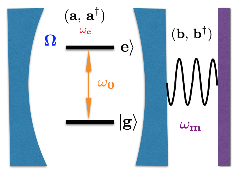
Figure 1: Schematic diagram of a cavity optomechanical system.

$$H =\omega\,a^{\dagger}a+\omega_{m}\,b^{\dagger}b+\tfrac{1}{2}\omega_{0}\sigma_{z}-G\,a^{\dagger}a(b+b^{\dagger})$$

$$\qquad\qquad\qquad\qquad+\Omega\,[a\,f(N)\,\sigma_{+}+f(N)\,a^{\dagger}\,\sigma_{-}].$$ (1)

Here $a^{\dagger},\,a$ and $b^{\dagger},\,b$ are, respectively, the creation and annihilation operators of the cavity mode with frequency $\omega$ and the mirror-oscillator unit with frequency $\omega_{m}$. $G=(2\,m\,\omega_{m}/\hbar)^{-1/2}\,(\omega/L)$ is the optomechanical coupling coefficient, where $L$ and $m$ are the length of the cavity and the mass of the mirror. $\sigma_{z}=\left|{e}\right\rangle\left\langle{e}\right|-\left|{g}\right\rangle\left\langle{g}\right|$,  $\sigma_{+}=\left|{e}\right\rangle\left\langle{g}\right|$ and $\sigma_{-}=\left|{g}\right\rangle\left\langle{e}\right|$, where $\left|{e}\right\rangle$ and $\left|{g}\right\rangle$ are, respectively, the excited and ground states of the atom. $\omega_{0}$ is the atomic transition frequency and $\Omega$ is the field-atom coupling constant. In our analysis, we have used the resonance condition $\omega=\omega_{0}+\omega_{m}$. The real-valued function $f(N)$ (where $N=a^{\dagger}a$) incorporates field-atom intensity-dependence.

As shown in Appendix A, an effective Hamiltonian $H_{\textrm{eff}}$ for this system can be obtained from $H$ in the limit $\omega_{m}\gg G,\,\Omega$. It is given by

$$H_{\textrm{eff}}= \frac{G\Omega}{\omega_{m}}\Big{[}f(N)a^{\dagger}\,b\,\sigma_{-}+af(N)b^{\dagger}\,\sigma_{+}\Big{]}$$

$$-\frac{\Omega^{2}}{\omega_{m}}\Big{[}a^{\dagger}a\,\sigma_{z}-\sigma_{+}\sigma_{-}\Big{]}-\frac{G^{2}}{\omega_{m}}\,(a^{\dagger}a)^{2}.$$ (2)

Note the emergence in $H_{\textrm{eff}}$ of (a) the intensity-dependent tripartite interaction between the atom, field and mirror (the terms proportional to $f(N)$ on the right-hand side), and (b) the Kerr nonlinearity in $H_{\textrm{eff}}$ (the last term on the right-hand side), although neither of these features is explicit in $H$. We start with an unentangled initial state of the system that is a direct product of the following states: (i) the field in a general superposition $\sum_{n=0}^{\infty}l_{n}\left|{n}\right\rangle$ of photon number states $\left|{n}\right\rangle$ (in contrast to Liao et al. (2016)); (ii) the mirror in the oscillator ground state $\left|{0}\right\rangle$; and (iii) the atom in an arbitrary superposition $(\cos\phi\left|{e}\right\rangle+\sin\phi\left|{g}\right\rangle)$. Thus

$$\left|{\psi(0)}\right\rangle=\sum_{n=0}^{\infty}l_{n}(\cos\phi\left|{n;0;e}\right\rangle+\sin\phi\left|{n;0;g}\right\rangle),$$ (3)

in an obvious notation. Solving the Schrödinger equation in the interaction picture, the state of the system at any instant of time is given by

$$\left|{\psi(t)}\right\rangle=\sum_{n=0}^{\infty} l_{n}A_{n}(t)\left|{n;0;e}\right\rangle+\sum_{n=0}^{\infty}l_{n}B_{n}(t)\left|{n;0;g}\right\rangle$$

$$\qquad\qquad\quad+\sum_{n=1}^{\infty}l_{n}C_{n}(t)\left|{n-1;1;e}\right\rangle,$$ (4)

where explicit expressions for the coefficients $A_{n}(t),B_{n}(t),C_{n}(t)$ and for the subsystem density operators are given in Appendix B.

III Entanglement dynamics

Let us now apply the foregoing to the case when the initial state of the field is a coherent state (CS) $\left|{\alpha}\right\rangle$ ($\alpha\in\mathbb{C}$), so that $l_{n}=\exp\,(-|\alpha|^{2}/2)\,(n!)^{-1/2}\,\alpha^{n}$. As we shall see, the dynamics is very sensitive to the specific form of the intensity dependence $f(N)$ of the tripartite coupling. Interesting features are exhibited by the entanglement (as characterized by the SVNE), squeezing properties, and the Wigner functions at specific instants of time.

In the investigations that follow, we choose experimentally realizable values of the relevant parameters. The typical cavity length $L$ is of the order of $\mu$m. Experiments have been carried out Hood et al. (1998) with cesium atoms passing through a cavity of length $L=10\,\mu$m, with atomic transition (6S_1/2, $F=4$, $m_{F}=4\longrightarrow$ 6P_3/2, $F=5$, $m_{F}=5$) and $\omega\sim 10^{14}$ Hz. Further, in such a set-up the mass $m$ of the oscillator is of the order of $10^{-17}$ kg, and the corresponding oscillator frequency $\omega_{m}$ is of the order of $10^{9}$ Hz Cleland and Roukes (1996). From this it follows that the value of the optomechanical coupling coefficients $G$ is $10^{6}$ Hz, which is much smaller than the value of $\omega_{m}$. The resonance condition $\omega=\omega_{0}+\omega_{m}$ is satisfied. Further, the coupling $\Omega$ between the atom and the cavity depends on the atomic position $r$ through the relation $\Omega=\Omega_{0}\,\exp(-r^{2}/w_{0}^{2})$, with the maximum value of the vacuum-Rabi frequency $\Omega_{0}=2\pi\times 120$ MHz and the waist of the cavity mode $w_{0}\approx 15\mu$m Hood et al. (1998). Hence, by adjusting $r$, the value of $\Omega$ can be set to be close to that of $G$. We examine two possibilities here, namely,   (a)  $G=\Omega$ and  (b)  $G=\sqrt{2}\,\Omega$. The latter choice is considered in order to examine whether qualitative features of the system dynamics are sensitive to changes in the ratio $G/\Omega$, because it has been reported earlier Liao et al. (2016) that the dynamics of the subsystem entropy is qualitatively different for these two values of the ratio concerned. We have examined in the following sections the manner in which both entropic and quadrature squeezing depend on the value of $G/\Omega$ during dynamical evolution. Since $G$ and $\Omega$ are comparable in their numerical values, the effective frequency ((2)) is given by $(G^{2}/\omega_{m})$. It is therefore natural to examine the dynamics in terms of the dimensionless time variable $\tau=(G^{2}/\omega_{m})t$.

III.1 Intensity-independent tripartite coupling

We consider first an intensity-independent tripartite coupling, which corresponds to setting $f(N)=1$. In figures 2(a)-(f), the SVNE for the atom (S${}_{\text{a}}$), mirror (S${}_{\text{m}}$) and field (S${}_{\text{f}}$) are plotted as functions of $\tau$, for $\Omega=10^{6}$. Two points are noteworthy. First, for $\phi=\tfrac{1}{2}\pi$, even for a small value of $\alpha$ (e.g., $\alpha=1$), S${}_{\text{a}}$ equals unity at specific instants of time (figure 2(a)). This is the maximum allowed value of the SVNE for a two-level atom. More importantly, with an increase in $\alpha$, this value remains constant over a long time interval (figure 2(b)). It follows from (B10)-(B12), (B) and (B) that for $\phi=\tfrac{1}{2}\pi$, the dynamics of S${}_{\text{a}}$ and S${}_{\text{m}}$ are identical. However, for other values of $\phi$ (e.g., $\tfrac{1}{4}\pi$), S${}_{\text{a}}$ does not collapse to a constant value over a significant time interval for any value of $\alpha$ (figures 2(a), (b)). In contrast, the SVNE for the oscillator subsystem collapses to a non-zero value ($<1$) over a significant time interval for sufficiently large $\alpha$ and for $\phi=\tfrac{1}{4}\pi$ (figure 2(d)). This allows for the possibility of tuning the values of $\alpha$ and $\phi$ to retain entanglement collapse over long time intervals. This could be potentially useful in quantum information transfer.

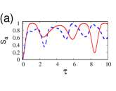
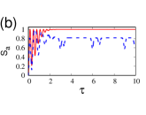
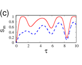
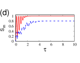
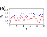
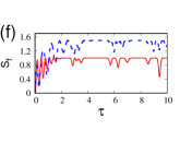
Figure 2: S${}_{\text{a}}$ (top panel), S${}_{\text{m}}$ (centre panel) and S${}_{\text{f}}$ (bottom panel) vs $\tau$, for $\Omega=10^{6}$ and $\phi=\tfrac{1}{2}\pi$ (red), $\tfrac{1}{4}\pi$ (blue). $\alpha=1$ (first column) and $5$ (second column).

We have also verified that a further enhancement of the interval over which such collapses occur is possible if we consider an initial field state $\left|{\alpha,m}\right\rangle$ ($m=1,\,2,\dotsc$), the $m$-photon added coherent state instead of a standard CS. $\left|{\alpha,\,m}\right\rangle$ is obtained Tara et al. (1993) by normalizing the state $(a^{\dagger})^{m}\left|{\alpha}\right\rangle$ to unity. The set $\{\left|{\alpha,\,m}\right\rangle\}$ provides a family of states whose departure from coherence is precisely quantifiable. We have verified that increasing $m$ increases the collapse interval.

No distinctive collapse in entanglement is seen in the field SVNE S${}_{\text{f}}$ for any value of $\alpha$ and $\phi$. Unlike S${}_{\text{a}}$ and S${}_{\text{m}}$, the largest value of S${}_{\text{f}}$ corresponds to $\phi=\tfrac{1}{4}\pi$ (figures 2(e)-(f)).

In contrast to the foregoing, when $\Omega$ is reduced to the value $10^{6}/\sqrt{2}$, relatively long-time-interval collapses of the SVNE to a non-zero value are observed for sufficiently large values of $\alpha$ for both $\phi=\tfrac{1}{2}\pi$ and $\tfrac{1}{4}\pi$ (figure 3(b),(d),(f)). For low values of $\alpha$ this feature is absent although relatively high values of SVNE are reached at specific instants of time.

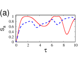
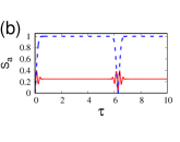
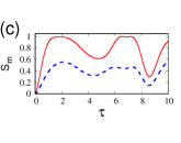
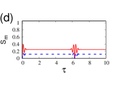
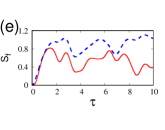
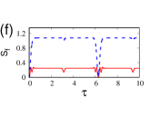
Figure 3: S${}_{\text{a}}$ (top panel), S${}_{\text{m}}$ (centre panel) and S${}_{\text{f}}$ (bottom panel) vs $\tau$, for $\Omega=10^{6}/\sqrt{2}$ and $\phi=\tfrac{1}{2}\pi$ (red), $\tfrac{1}{4}\pi$ (blue). $\alpha=1$ (first column) and $5$ (second column).

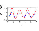
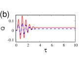
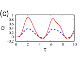
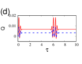
Figure 4: Mandel Q parameter vs $\tau$ for $\phi=\tfrac{1}{2}\pi$ (red), $\tfrac{1}{4}\pi$ (blue). $\alpha=1$ (first column) and $5$ (second column). $\Omega=10^{6}$ (top panel) and $10^{6}/\sqrt{2}$ (bottom panel).

The Mandel Q parameter for the field subsystem displays collapse over a long time interval for both $\Omega=10^{6}$ and $\Omega=10^{6}/\sqrt{2}$ for sufficiently high $\alpha$ (figures 4(b), (d)). Such collapses are not present for small $\alpha$ (figures 4(a), (c)). We see sub-Poissonian signatures (negative values) of Q in all cases. However, for smaller $\alpha$, these are more prominent. We have verified that these features are also reflected in the dynamics of the mean photon number, its variance and the atomic inversion parameter.

III.2 Intensity-dependent tripartite coupling

The results presented in the foregoing enable us to infer that entanglement collapses of SVNE to non-zero values over a long time interval are present only for sufficiently large values of $\alpha$. We now examine how various forms of IDC affect the collapse intervals of S${}_{\text{a}}$ and S${}_{\text{m}}$.

We find that, when $f(N)=(a^{\dagger}a)^{-1/2}$ collapses are destroyed, while for $f(N)=(a^{\dagger}a)^{1/2}$ the collapse intervals are reduced, compared to the intensity-independent situation. For $f(N)=(1+\kappa\,a^{\dagger}a)^{1/2}$ ($0<\kappa\leq 1)$, an increase in $\kappa$ decreases the interval of collapse, but increases the number of collapses within a given time interval. Figures 5(a)-(c) show contour plots of the SVNE as a function of $\tau$ and the IDC parameter $\kappa$.

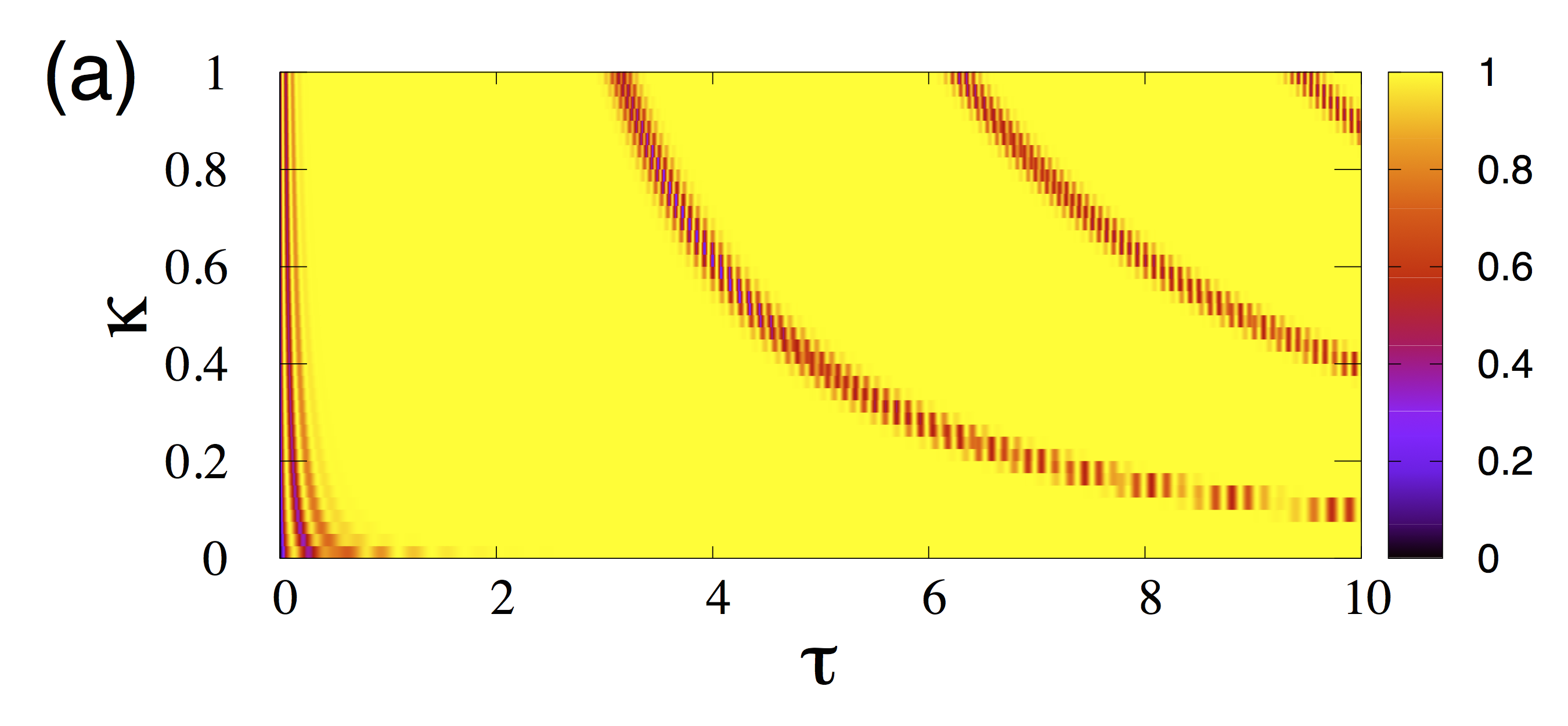
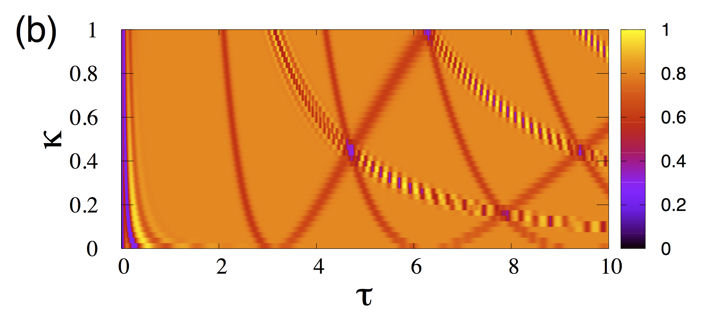
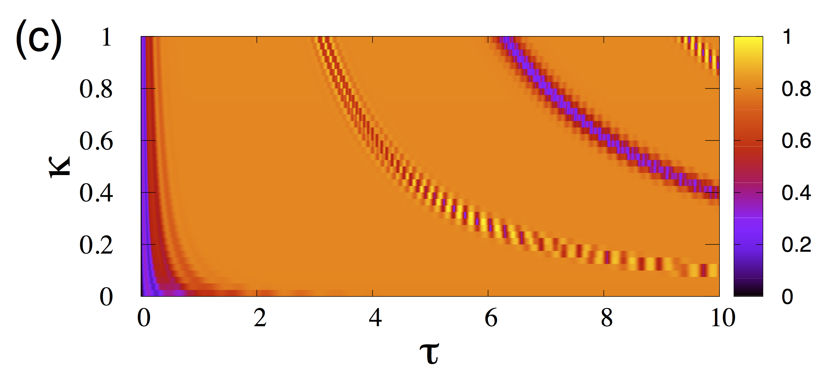
Figure 5: Contour plots of SVNE vs $\tau$ and $\kappa$ with $\alpha=8$ and $\Omega=10^{6}$, for (a) the atom and the oscillator for $\phi=\tfrac{1}{2}\pi$; (b) the atom for $\phi=\tfrac{1}{4}\pi$; (c) the oscillator for $\phi=\tfrac{1}{4}\pi$.

We now compare these results with those obtained for a $\Lambda$ atom interacting with a coupling field and a probe field Laha et al. (2016). In both systems, the SVNE collapses to a constant non-zero value over a significant interval of time in the absence of intensity-dependent field-atom coupling, and the dynamics is very sensitive to the value of the parameter $\kappa$. In the latter system, an increase in $\kappa$ produced a spectacular bifurcation cascade in the qualitative behaviour of the SVNE. While such remarkable changes do not appear in the present model, there are still distinctive features in the SVNE that are controlled by the precise value of $\kappa$ (figures 5(a)-(c)). Additionally, in the case at hand, the SVNE collapses to its maximum possible value, as explained earlier.

Finally, we observe in passing that for $f(N)=(a^{\dagger}a)^{-1/2}$ (and $\Omega=10^{6}$), the Q parameter for the field does not become negative over the time interval considered for any value of $\alpha$ and $\phi$, in contrast to its behaviour for $f(N)=(a^{\dagger}a)^{1/2}$ or $(1+\kappa\,a^{\dagger}a)^{1/2}$.

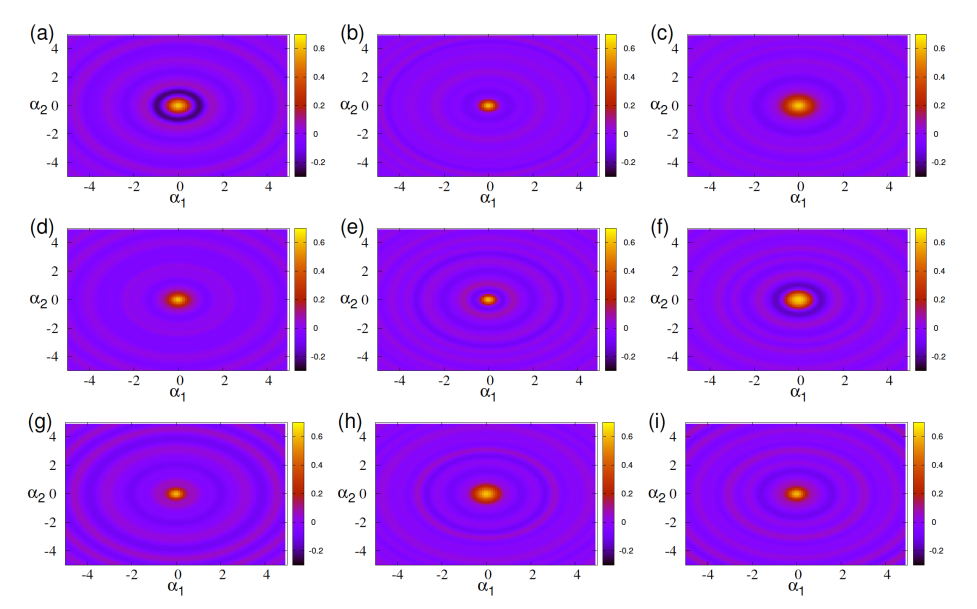
Figure 6: $W_{f}(\alpha)$ vs $\alpha_{1}$ and $\alpha_{2}$ for $\phi=\tfrac{1}{2}\pi$, $\Omega=10^{6}$ and $f(N)=(1+\kappa\,a^{\dagger}a)^{1/2}$ for $\kappa=0$ (top panel), $0.5$ (middle panel) and $1$ (bottom panel) at instants $\tau=2$ (first column), $5$ (second column) and $8$ (third column) respectively.

III.3 Wigner functions of the field

The nonclassical nature of the field at various instants of time is reflected in the negativity of the Wigner functions at those instants. We have derived an expression for the Wigner distribution $W_{f}(\alpha)$ ($\alpha=\alpha_{1}+i\,\alpha_{2}$) in Appendix C. For the generic state given in (4), we have

$$W_{f}(\alpha) =\frac{2}{\pi}\sum_{n,k,l=0}^{\infty}(-1)^{n}\,q_{k}\,q_{l}^{*}\big{[}A_{k}\,A_{l}^{*}+B_{k}\,B_{l}^{*}\big{]}\times$$

$$\hskip 113.81102pt\left\langle{n}\right|{D^{\dagger}}\left|{k}\right\rangle\left\langle{l}\right|{D^{\dagger}}\left|{n}\right\rangle$$

$$+\frac{2}{\pi}\sum_{n,k,l=0}^{\infty}(-1)^{n}\,q_{k}\,q_{l}^{*}C_{k}\,C_{l}^{*}\times$$

$$\hskip 56.9055pt\left\langle{n}\right|{D^{\dagger}}\left|{k-1}\right\rangle\left\langle{l-1}\right|{D^{\dagger}}\left|{n}\right\rangle,$$ (5)

with the identification

$$\left\langle{n}\right|{D}\left|{m}\right\rangle=\left\{\begin{array}[]{l}e^{-\frac{1}{2}|\alpha|^{2}}\,\sqrt{\frac{m!}{n!}}\,\,\alpha^{n-m}\,L_{m}^{n-m}(|\alpha|^{2})\;\;(n\geq m)\\[6.0pt] e^{-\frac{1}{2}|\alpha|^{2}}\,\sqrt{\frac{n!}{m!}}\,\,(-\alpha^{*})^{m-n}\,L_{n}^{m-n}(|\alpha|^{2})\;\;(n<m)\end{array}\right.$$ (6)

where $L_{n}^{m}(x)$ is the associated Laguerre polynomial. Here $A_{i},\,B_{i}$ and $C_{i}$ are functions of both time and $f(N)$.

For completeness, we plot the Wigner functions for different values of $\tau$ and $\kappa$ in figures 6(a)-(i). It is evident that for a fixed value of $\kappa$ , negativity of the Wigner function does not necessarily increase with time (see for instance, figures 6(d)-(f)).

IV The optical tomogram and squeezing properties of the field

IV.1 The optical tomogram

We now examine the squeezing of the state of the field subsystem as the full system evolves in time. It is useful to carry out this analysis in terms of the optical tomogram $\omega(X_{\theta},\theta)$ of the field, because the nonclassical properties of the field are conveniently reflected in this quantity: $\omega(X_{\theta},\theta)$ is just the Radon transform of the Wigner function $W(p,q)$ derived in Appendix C. It is defined as

$$\omega(X_{\theta},\theta)=\int\delta(\mathbb{X}_{\theta}-X_{\theta}\mathbb{I})\,W(p,q)\,\frac{dq\,dp}{2\pi},$$ (7)

where $\mathbb{I}$ is the identity operator, and

$$\mathbb{X}_{\theta}=\hat{q}\cos\theta+\hat{p}\sin\theta=(ae^{-i\theta}+a^{\dagger}e^{i\theta})/\sqrt{2}$$ (8)

is the homodyne quadrature operator expressed in terms of the photon destruction and creation operators. We have $\mathbb{X}_{\theta}\left|{X_{\theta},\theta}\right\rangle=X_{\theta}\left|{X_{\theta},\theta}\right\rangle$, where

$$\left|{X_{\theta},\theta}\right\rangle=\frac{1}{\sqrt{\pi}}\exp\,\big{(}\!-\tfrac{1}{2}X_{\theta}^{2}-\tfrac{1}{2}e^{i2\theta}a^{\dagger 2}+\sqrt{2}e^{i\theta}X_{\theta}a^{\dagger}\big{)}\left|{0}\right\rangle.$$ (9)

We make use of the fact that $\omega(X_{\theta},\theta)=\left\langle{X_{\theta},\theta}\right|{\rho_{f}}\left|{X_{\theta},\theta}\right\rangle$. It follows that, for a state $\left|{\psi}\right\rangle=\sum_{n=0}^{\infty}c_{n}\left|{n}\right\rangle$,

$$\omega(X_{\theta},\theta)=\frac{e^{-X_{\theta}^{2}}}{\sqrt{\pi}}\Bigg{|}\sum_{n=0}^{\infty}c_{n}\frac{e^{-in\theta}}{\sqrt{2^{n}\>n!}}H_{n}(X_{\theta})\Bigg{|}^{2}.$$ (10)

($H_{n}$ is the Hermite polynomial of order $n$.) In what follows, (10) will be used extensively for numerically estimating the squeezing properties of the field from the tomogram.

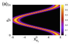
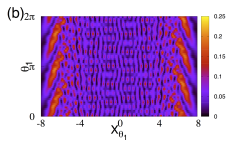
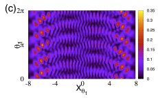
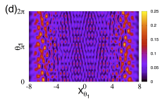
Figure 7: Field tomograms at (a) $\tau=0$, (b) $\tau=2$, (c) $\tau=5$ and (d) $\tau=8$, for $\Omega=10^{6},\,\phi=\tfrac{1}{2}\pi,\,\alpha=5,\,\kappa=0$ for an initial CS.

The generic tomogram is pictorially represented as an intensity plot of $\omega(X_{\theta},\theta)$ versus $X_{\theta}$ and $\theta$. In figure 7(a) we present the tomogram of an initial CS with $\alpha=5$. In contrast to this, the tomograms at later times are significantly more complex in appearance: this is illustrated, for the sake of completeness, in figures 7(b-d). These tomograms correspond to the Wigner functions at the instants specified in figures 6(a-c).

IV.2 Entropic and quadrature squeezing

The tomographic entropy $S(\theta)$ for a subsystem, defined as

$$S(\theta)=-\int\omega(X_{\theta},\theta)\,\ln\,[\omega(X_{\theta},\theta)]\,dX_{\theta},$$ (11)

satisfies the entropic uncertainty relation (EUR) Orłowski (1997)

$$S(\theta)+S(\theta+\tfrac{1}{2}\pi)\geq\ln\,(\pi e)$$ (12)

at every instant of time. A state with entropy in either quadrature ($\theta$ or $\theta+\tfrac{1}{2}\pi$) less than $\tfrac{1}{2}\ln\,(\pi e)$ displays entropic squeezing in that quadrature. The optical tomogram $\omega(X_{\theta},\theta)$ is non-negative, and satisfies $\int\omega(X_{\theta},\theta)\,dX_{\theta}=1$. Hence, we can calculate the moments of the quadrature operators from $\omega(X_{\theta},\theta)$ in a straightforward manner. For any specific value of $\theta$, we have

$$\left\langle{X^{n}}\right\rangle=\int X^{n}\,\omega(X_{\theta},\theta)\,dX_{\theta}.$$ (13)

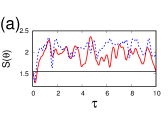
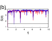
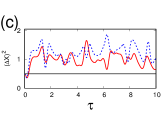
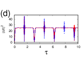
Figure 8: $S(\theta)$ (top panel) and $(\Delta X)^{2}$ (bottom panel) vs $\tau$ for $\Omega=10^{6}$, $\theta=0$, $\phi=\tfrac{1}{2}\pi$ (red) and $\phi=\tfrac{1}{4}\pi$ (blue). $\alpha=1$ (first column) and $5$ (second column). The horizontal black line is the reference value below which squeezing occurs.

For $\Omega=10^{6}$ and $\theta=0$, for instance, the tomographic entropy is squeezed for $\alpha=1$ although only at a few instants (figure 8(a)). With an increase in the value of $\alpha$, the extent of squeezing does not significantly change (compare figures 8(a), (b)). Variances in quadrature operators are also not significantly squeezed for these values of the parameters, except at a few instants (figures 8(c), (d)). In contrast, for $\Omega=10^{6}/\sqrt{2}$, the tomographic entropy exhibits more squeezing during the time interval considered (figures 9(a)-(b)).

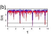
Figure 9: $S(\theta)$ vs $\tau$ for $\Omega=10^{6}/\sqrt{2}$, $\theta=0$, $\phi=\tfrac{1}{2}\pi$ (red) and $\phi=\tfrac{1}{4}\pi$ (blue). (a) $\alpha=1$, (b) $\alpha=5$. The horizontal black line is the reference value below which squeezing occurs.

For completeness, we report that over the same interval of time ($0\leq\tau\leq 10$) and $f(N)=(a^{\dagger}a)^{1/2}$, the state displays entropic squeezing more frequently for $\Omega=10^{6}$ and less frequently for $\Omega=10^{6}/\sqrt{2}$ as $\alpha$ is increased. For $f(N)=(a^{\dagger}a)^{-1/2}$, the frequency with which squeezing occurs increases with increasing $\alpha$ for both values of $\Omega$.

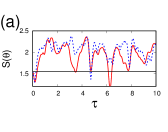
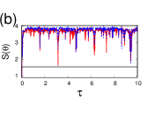
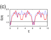
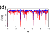
Figure 10: $S(\theta)$ vs $\tau$ for $\Omega=10^{6},\,\theta=0$. $\phi=\tfrac{1}{2}\pi$ (red) and $\phi=\tfrac{1}{4}\pi$ (blue). $\alpha=1$ (first column), $\alpha=5$ (second column). $\kappa=0.5$ (top panel), $\kappa=1$ (bottom panel). The red horizontal line is the reference below which squeezing occurs.

For $f(N)=(1+\kappa\,a^{\dagger}a)^{1/2}$ ($0\leq\kappa\leq 1$) and over the same time interval, there is a remarkable difference in the qualitative behaviour in the dynamics of both the tomographic entropy (figures 10(a)-(d)) and the quadrature observables. In particular, squeezing properties are very sensitive to the value of $\kappa$, and even small changes in $\kappa$ lead to substantial changes in them. This is evident in the case of entropic squeezing where for a sufficiently high value of $\alpha$, the extent of squeezing varies significantly with $\kappa$ (figures 10(b), (d) in which the tomographic entropy is plotted against time for $\Omega=10^{6}$). Such sensitive dependence on $\kappa$ is not observed for $\Omega=10^{6}/\sqrt{2}$.

V Concluding remarks

We have investigated, in some detail, the dynamics of the subsystem von Neumann entropy for the different subsystems of a generic optomechanical model. We have established that the SVNE of the atom collapses to its maximum allowed value over a significant interval of time, as opposed to sudden death of entanglement. This novel feature is potentially useful in harnessing entanglement protocols. We have explored experimentally viable parameter regimes and examined how different intensity-dependent couplings affect the nonclassical nature of the radiation field. We have assessed the extent of nonclassicality of the cavity field during time evolution through the Mandel Q parameter, the Wigner functions and the corresponding optical tomograms. Finally, we have quantified entropic and quadrature squeezing properties directly from the field tomograms, thus by-passing inherently error-prone state reconstruction methods. It is hoped that our study provides pointers to several aspects of the dynamical behaviour of a variety of optomechanical systems.

Appendix A The effective Hamiltonian

The Hamiltonian $H$ in (1) can be written as $H_{0}+H_{1}$, where

$$H_{0} =\omega\,a^{\dagger}a+\omega_{m}\,b^{\dagger}b+\tfrac{1}{2}\omega_{0}\sigma_{z},$$ (A1)

$$H_{1} =-G\,a^{\dagger}a(b+b^{\dagger})+\Omega\,[a\,f(N)\,\sigma_{+}+f(N)\,a^{\dagger}\,\sigma_{-}].$$ (A2)

We express any operator $A_{I}(t)$ in the interaction picture as $e^{iH_{0}t}\,A\,e^{-iH_{0}t}$, where $A$ is the operator in the Schrödinger picture, and use the identities

$$N^{r}\,a=a(N-1)^{r},\;\;\sigma_{z}^{r}\,\sigma_{-}=\sigma_{-}\,(\sigma_{z}-2)^{r}\;(r=1,2,\cdots)$$ (A3)

to obtain

$$a_{I}=a\,e^{-i\omega t},\;\;b_{I}=b\,e^{-i\omega_{m}t},\;\;(\sigma_{-})_{I}=\sigma_{-}\,e^{-i\omega_{0}t}.$$ (A4)

Dropping the subscript $I$ and using the resonance condition $\omega=\omega_{m}+\omega_{0}$, we get, in terms of interaction picture operators,

$$H_{\textrm{int}}= \Omega\,\big{[}a\,f(N)\,\sigma_{+}\,e^{-i\omega_{m}t}+f(N)\,a^{\dagger}\,\sigma_{-}\,e^{i\omega_{m}t}\big{]}$$

$$\qquad\qquad-G\,a^{\dagger}a\,\big{[}b\,e^{-i\omega_{m}t}+b^{\dagger}\,e^{i\omega_{m}t}\big{]}.$$ (A5)

As is well known, in coarse-grained dynamics in which rapidly oscillating terms are neglected in the rotating-wave approximation, a generic Hamiltonian of the form

$$\mathcal{H}_{\textrm{I}}=\sum_{n=1}^{N}(h_{n}\,e^{-i\omega_{n}t}+h_{n}^{\dagger}\,e^{i\omega_{n}t})$$ (A6)

can be recast into an effective Hamiltonian of the form James and Jerke (2007)

$$\mathcal{H}_{\textrm{eff}}=\sum_{n=1}^{N}\sum_{m=1}^{N}\ (\overline{\omega}_{mn})^{-1}\,[h_{m}^{\dagger},h_{n}]\,e^{i(\omega_{m}-\omega_{n})t},$$ (A7)

where $\overline{\omega}_{mn}=2\,\omega_{m}\,\omega_{n}/(\omega_{m}+\omega_{n})$. We follow a similar procedure, since $\omega_{m}\gg(G,\,\Omega)$, and the approximation holds good in this case too. With the identifications

$$h_{1}=-G\,a^{\dagger}a\,b,\;\;h_{2}=\Omega\,af(N)\,\sigma_{+},\;\;\overline{\omega}_{mn}=\omega_{m},$$ (A8)

it is easy to see that

$$[h_{1}^{\dagger},\,h_{1}] =G^{2}\,(a^{\dagger}a)^{2},\;\;[h_{1}^{\dagger},\,h_{2}]=G\,\Omega\,a\,f(N)\,b^{\dagger},$$ (A9)

$$[h_{2}^{\dagger},h_{2}] =-\Omega^{2}\big{[}a^{\dagger}af^{2}(n)\,\sigma_{z}+\big{\{}af^{2}(N)a^{\dagger}$$

$$\hskip 85.35826pt-a^{\dagger}af^{2}(N)\big{\}}\sigma_{+}\sigma_{-}\big{]}.$$ (A10)

The effective Hamiltonian can now be written as

$$H_{\textrm{eff}} =\frac{G\Omega}{\omega_{m}}\big{[}f(N)a^{\dagger}\,b\,\sigma_{-}+af(N)b^{\dagger}\,\sigma_{+}\big{]}-\frac{G^{2}}{\omega_{m}}\,(a^{\dagger}a)^{2}$$

$$-\frac{\Omega^{2}}{\omega_{m}}\big{[}a^{\dagger}a\,f^{2}(N)\sigma_{z}+\big{\{}af^{2}(N)\,a^{\dagger}-a^{\dagger}a\,f^{2}(N)\big{\}}\,\sigma_{+}\sigma_{-}\big{]}.$$ (A11)

To first order in the intensity-dependent coupling $f(N)$ (approximating the square $f^{2}(N)$ by unity), we arrive at the effective Hamiltonian

$$H_{\textrm{eff}} =\frac{G\Omega}{\omega_{m}}\big{[}f(N)a^{\dagger}\,b\,\sigma_{-}+af(N)b^{\dagger}\,\sigma_{+}\big{]}$$

$$-\frac{\Omega^{2}}{\omega_{m}}\big{[}a^{\dagger}a\,\sigma_{z}-\sigma_{+}\sigma_{-}\big{]}-\frac{G^{2}}{\omega_{m}}\,(a^{\dagger}a)^{2}.$$ (A12)

Appendix B The state vector

The initial state given by (3) is

$$\left|{\psi(0)}\right\rangle=\sum_{n=0}^{\infty}l_{n}(\cos\phi\left|{n;0;e}\right\rangle+\sin\phi\left|{n;0;g}\right\rangle).$$ (B1)

Its temporal evolution is governed by $H_{\textrm{eff}}$ ((2)). We have

$$\left|{\psi(t)}\right\rangle=\sum_{n=0}^{\infty} l_{n}A_{n}(t)\left|{n;0;e}\right\rangle+\sum_{n=0}^{\infty}l_{n}B_{n}(t)\left|{n;0;g}\right\rangle$$

$$+\sum_{n=1}^{\infty}l_{n}C_{n}(t)\left|{n-1;1;e}\right\rangle,$$ (B2)

where the time derivatives of the coefficients are obtained from the Schrödinger equation:

$$\dot{A}_{n}(t) =pA_{n}(t),$$ (B3)

$$\dot{B}_{n}(t) =qB_{n}(t)+sC_{n}(t),$$ (B4)

$$\dot{C}_{n}(t) =rC_{n}(t)+sB_{n}(t),$$ (B5)

where

$$p =i[G\Omega\,n^{2}+\Omega^{2}(n+1)]/{\omega_{m}},$$ (B6)

$$q =i[G\Omega\,(n-1)^{2}+\Omega^{2}n]/{\omega_{m}},$$ (B7)

$$r =i[G^{2}\,n^{2}-\Omega^{2}\,n]/{\omega_{m}},$$ (B8)

$$s =-iG\Omega\,f(n)\sqrt{n}/{\omega_{m}}.$$ (B9)

We impose the initial conditions $A_{n}(0)=\cos\phi$, $B_{n}(0)=\sin\phi$ and $C_{n}(0)=0$, and solve the equations given above to get

$$A_{n}(t) =\cos\,\phi\,e^{\,i\gamma_{1}t},$$ (B10)

$$B_{n}(t) =\sin\,\phi\,\big{[}\cos\,(Rt)+\Delta_{b}\sin\,(Rt)\big{]}\,e^{\,i\gamma_{2}t},$$ (B11)

$$C_{n}(t) =\sin\phi\,\sin(Rt)\,\Delta_{c}\,e^{\,i\gamma_{2}t},$$ (B12)

where

$$\gamma_{1} =\big{[}G^{2}n^{2}+(n+1)\Omega^{2}\big{]}/{\omega_{m}},$$ (B13)

$$\gamma_{2} =G^{2}\big{(}n^{2}-n+\tfrac{1}{2}\big{)}/{\omega_{m}},$$ (B14)

$$\Delta_{b} =-i[G^{2}\,(n-\tfrac{1}{2})-\Omega^{2}\,n]/{(R\omega_{m})},$$ (B15)

$$\Delta_{c} =-iG\,\Omega\,\sqrt{n}\,f(n)/{(R\omega_{m})},$$ (B16)

$$R =\Big{\{}\tfrac{1}{4}G^{4}(2n^{2}-2n+1)^{2}+G^{2}\Omega^{2}\,n\,f^{2}(n)$$

$$\quad-[G^{2}\,(n-1)^{2}+\Omega^{2}\,n][G^{2}n^{2}-\Omega^{2}\,n]\Big{\}}^{1/2}/{\omega_{m}}.$$ (B17)

The respective reduced density matrices for the atom, the mirror and the field are then given by

$$\rho_{a} =\sum_{n=0}^{\infty}\Big{[}\Big{(}|l_{n}|^{2}\,|A_{n}|^{2}+|l_{n+1}|^{2}|C_{n+1}|^{2}\Big{)}\left|{e}\right\rangle\left\langle{e}\right|$$

$$+|l_{n}|^{2}\Big{(}|B_{n}|^{2}\left|{g}\right\rangle\left\langle{g}\right|+A_{n}B_{n}^{*}\left|{e}\right\rangle\left\langle{g}\right|+A_{n}^{*}B_{n}\left|{g}\right\rangle\left\langle{e}\right|\Big{)}\Big{]},$$ (B18)

$$\rho_{m} =\sum_{n=0}^{\infty}\Big{[}|l_{n}|^{2}\Big{(}|A_{n}|^{2}+|B_{n}|^{2}\Big{)}\left|{0}\right\rangle\left\langle{0}\right|+|l_{n+1}|^{2}|C_{n+1}|^{2}\left|{1}\right\rangle\left\langle{1}\right|$$

$$\quad\,\,\,\,+l_{n}l_{n+1}^{*}A_{n}C_{n+1}^{*}\left|{0}\right\rangle\left\langle{1}\right|+l_{n}^{*}l_{n+1}A_{n}^{*}C_{n+1}\left|{1}\right\rangle\left\langle{0}\right|\Big{]},$$ (B19)

$$\rho_{f} =\sum_{n=0}^{\infty}\sum_{m=0}^{\infty}l_{n}l_{m}^{*}[A_{n}A_{m}^{*}+B_{n}B_{m}^{*}]\left|{n}\right\rangle\left\langle{m}\right|$$

$$\qquad+\sum_{n=1}^{\infty}\sum_{m=1}^{\infty}l_{n}l_{m}^{*}C_{n}C_{m}^{*}\left|{n-1}\right\rangle\left\langle{m-1}\right|,$$ (B20)

where the coefficients $A_{n},\,B_{n},\,C_{n}$ have the time dependences indicated in (B10)–(B12).

Appendix C The Wigner function for the field

The Wigner function $W(p,\,q)$ for a state with density matrix $\rho_{f}$ is defined by the integral Ghorbani et al. (2017)

$$W(p,\,q)=\frac{1}{\pi}\int_{-\infty}^{\infty}\,dq^{\prime}\left\langle{q+q^{\prime}}\right|{\rho_{f}}\left|{q-q^{\prime}}\right\rangle e^{-2i\,p\,q^{\prime}}$$ (C1)

in standard notation. We now use the fact that $e^{-i\,\hat{p}\,x}\left|{q}\right\rangle=\left|{q+x}\right\rangle$, and the identity $\displaystyle{e^{\hat{A}+\hat{B}}=e^{-\frac{1}{2}[\hat{A},\,\hat{B}]}\,e^{\hat{A}}\,e^{\hat{B}}}$ (since $[\hat{A},\,\hat{B}]$ is proportional to the unit operator in the cases of interest here). It is straightforward to see that

$$D(\alpha)\left|{-q^{\prime}}\right\rangle =e^{-\frac{1}{2}i\,qp}e^{i\,p\,\hat{q}}e^{-i\,q\,\hat{p}}\left|{q-q^{\prime}}\right\rangle$$

$$=e^{\frac{1}{2}i\,qp}e^{-i\,p\,q^{\prime}}\left|{q-q^{\prime}}\right\rangle,$$ (C2)

where $D(\alpha)=e^{\alpha a^{\dagger}-\alpha^{*}a}=e^{ip\hat{q}-iq\hat{p}}$ is the displacement operator. Inverting (C2), we have

$$\left|{q-q^{\prime}}\right\rangle=e^{-i\,q\,p/2}\,e^{i\,p\,q^{\prime}}\,D(\alpha)\left|{-q^{\prime}}\right\rangle.$$ (C3)

Substituting (C3) and its Hermitian conjugate in (C1), we get

$$W(\alpha) =(1/\pi)\int_{-\infty}^{\infty}\,dq^{\prime}\left\langle{q^{\prime}}\right|{D^{\dagger}(\alpha)\,\rho_{f}\,D(\alpha)}\left|{-q^{\prime}}\right\rangle$$

$$=(2/\pi)\int_{0}^{\infty}\,dq^{\prime}\left\langle{q^{\prime}}\right|{D^{\dagger}(\alpha)\,\rho_{f}\,D(\alpha)}\left|{-q^{\prime}}\right\rangle.$$ (C4)

Inserting the identity operator $\sum_{n=0}^{\infty}\left|{n}\right\rangle\left\langle{n}\right|$ in (C4) and using the fact that $\left\langle{n}|{-q}\right\rangle=(-1)^{n}\left\langle{n}|{q}\right\rangle$, we obtain

$$W(\alpha)=(2/\pi)\sum_{n=0}^{\infty}(-1)^{n}\left\langle{n;\,\alpha}\right|{\rho_{f}}\left|{n;\,\alpha}\right\rangle,$$ (C5)

where $\left|{n;\,\alpha}\right\rangle=D(\alpha)\left|{n}\right\rangle$ is a displaced number state (or a generalized coherent state). Using (C5), the expression in (5) for the Wigner function $W_{f}(\alpha)$ corresponding to the density matrix $\rho_{f}$ given by (B) is obtained easily.

References

- Aspelmeyer et al. (2014) M. Aspelmeyer, T. J. Kippenberg, and F. Marquardt, Rev. Mod. Phys. 86, 1391 (2014).
- Bowen and Milburn (2016) W. P. Bowen and G. J. Milburn, Quantum Optomechanics (CRC Press, 2016).
- Abramovici et al. (1992) A. Abramovici, W. E. Althouse, R. W. P. Drever, Y. Gürsel, S. Kawamura, F. J. Raab, D. Shoemaker, L. Sievers, R. E. Spero, K. S. Thorne, R. E. Vogt, R. Weiss, S. E. Whitcomb, and M. E. Zucker, Science 256, 325 (1992).
- Braginsky V B and S (1995) K. F. Y. Braginsky V B and T. K. S, Quantum measurement (Cambridge University Press, 1995).
- Vitali et al. (2001) D. Vitali, S. Mancini, and P. Tombesi, Phys. Rev. A 64, 051401 (2001).
- Geraci et al. (2010) A. A. Geraci, S. B. Papp, and J. Kitching, Phys. Rev. Lett. 105, 101101 (2010).
- Lamoreaux (2007) S. K. Lamoreaux, Phys. Today 60, 40 (2007).
- Stannigel et al. (2010) K. Stannigel, P. Rabl, A. S. Sørensen, P. Zoller, and M. D. Lukin, Phys. Rev. Lett. 105, 220501 (2010).
- Barzanjeh et al. (2011) S. Barzanjeh, M. H. Naderi, and M. Soltanolkotabi, Phys. Rev. A 84, 023803 (2011).
- Wilson-Rae et al. (2004) I. Wilson-Rae, P. Zoller, and A. Imamoḡlu, Phys. Rev. Lett. 92, 075507 (2004).
- Genes et al. (2008a) C. Genes, D. Vitali, P. Tombesi, S. Gigan, and M. Aspelmeyer, Phys. Rev. A 77, 033804 (2008a).
- Li et al. (2008) Y. Li, Y.-D. Wang, F. Xue, and C. Bruder, Phys. Rev. B 78, 134301 (2008).
- Schwab and Roukes (2005) K. C. Schwab and M. L. Roukes, Phys. Today 58, 36 (2005).
- Marshall et al. (2003) W. Marshall, C. Simon, R. Penrose, and D. Bouwmeester, Phys. Rev. Lett. 91, 130401 (2003).
- Rashid et al. (2017) M. Rashid, M. Toroš, and U. Hendrik, Quantum Meas. Quantum Metrol. 4, 17 (2017).
- Toroš et al. (2018) M. Toroš, M. Rashid, and H. Ulbricht, ArXiv:1804.01150 quant-ph (2018).
- Genes et al. (2008b) C. Genes, D. Vitali, and P. Tombesi, Phys. Rev. A 77, 050307 (2008b).
- Liu et al. (2013) N. Liu, J. Li, and J.-Q. Liang, Int. J. Th. Phys. 52, 706 (2013).
- Liao et al. (2016) Q. H. Liao, W. J. Nie, J. Xu, Y. Liu, N. R. Zhou, Q. R. Yan, A. Chen, N. H. Liu, and M. A. Ahmad, Laser Phys. 26, 055201 (2016).
- Nadiki and Tavassoly (2016) M. H. Nadiki and M. K. Tavassoly, Laser Phys. 26, 125204 (2016).
- Hammerer et al. (2009) K. Hammerer, M. Wallquist, C. Genes, M. Ludwig, F. Marquardt, P. Treutlein, P. Zoller, J. Ye, and H. J. Kimble, Phys. Rev. Lett. 103, 063005 (2009).
- Wallquist et al. (2010) M. Wallquist, K. Hammerer, P. Zoller, C. Genes, M. Ludwig, F. Marquardt, P. Treutlein, J. Ye, and H. J. Kimble, Phys. Rev. A 81, 023816 (2010).
- Buck and Sukumar (1981) B. Buck and C. Sukumar, Phys. Lett. A 81, 132 (1981).
- Sudarshan (1993) E. C. G. Sudarshan, Int. J. Th. Phys. 32, 1069 (1993).
- Laha et al. (2016) P. Laha, B. Sudarsan, S. Lakshmibala, and V. Balakrishnan, Int. J. Th. Phys. 55, 4044 (2016).
- Sivakumar (2002) S. Sivakumar, J. Phys. A: Math. Gen. 35, 6755 (2002).
- Nicola et al. (2007) S. D. Nicola, R. Fedele, M. A. Man’ko, and V. I. Man’ko, Journal of Physics: Conference Series 70, 012007 (2007).
- De Nicola et al. (2007) S. De Nicola, R. Fedele, M. A. Man’ko, and V. I. Man’ko, Theor. Math. Phys. 152, 1081 (2007).
- Ibort et al. (2009) A. Ibort, V. I. Man’ko, G. Marmo, A. Simoni, and F. Ventriglia, Phys. Scr. 79, 065013 (2009).
- Smithey et al. (1993) D. T. Smithey, M. Beck, M. G. Raymer, and A. Faridani, Phys. Rev. Lett. 70, 1244 (1993).
- Schiller et al. (1996) S. Schiller, G. Breitenbach, S. F. Pereira, T. Müller, and J. Mlynek, Phys. Rev. Lett. 77, 2933 (1996).
- Rohith and Sudheesh (2015) M. Rohith and C. Sudheesh, Phys. Rev. A 92, 053828 (2015).
- Sharmila et al. (2017) B. Sharmila, K. Saumitran, S. Lakshmibala, and V. Balakrishnan, J. Phys. B: At. Mol. Opt. Phys. 50, 045501 (2017).
- Rohith and Sudheesh (2016) M. Rohith and C. Sudheesh, J. Opt. Soc. Am. B 33, 126 (2016).
- Laha et al. (2018) P. Laha, S. Lakshmibala, and V. Balakrishnan, J. Mod. Opt. 65, 1466 (2018).
- Hood et al. (1998) C. J. Hood, M. S. Chapman, T. W. Lynn, and H. J. Kimble, Phys. Rev. Lett. 80, 4157 (1998).
- Cleland and Roukes (1996) A. N. Cleland and M. L. Roukes, Appl. Phys. Lett. 69, 2653 (1996).
- Tara et al. (1993) K. Tara, G. S. Agarwal, and S. Chaturvedi, Phys. Rev. A 47, 5024 (1993).
- Orłowski (1997) A. Orłowski, Phys. Rev. A 56, 2545 (1997).
- James and Jerke (2007) D. F. James and J. Jerke, Can. J. Phys. 85, 625 (2007).
- Ghorbani et al. (2017) M. Ghorbani, M. J. Faghihi, and H. Safari, J. Opt. Soc. Am. B 34, 1884 (2017).