A Unified Framework for Efficient Estimation of General Treatment Models

Abstract

This paper presents a weighted optimization framework that unifies the binary, multi-valued, continuous, as well as mixture of discrete and continuous treatment, under the unconfounded treatment assignment. With a general loss function, the framework includes the average, quantile and asymmetric least squares causal effect of treatment as special cases. For this general framework, we first derive the semiparametric efficiency bound for the causal effect of treatment, extending the existing bound results to a wider class of models. We then propose a generalized optimization estimation for the causal effect with weights estimated by solving an expanding set of equations. Under some sufficient conditions, we establish consistency and asymptotic normality of the proposed estimator of the causal effect and show that the estimator attains our semiparametric efficiency bound, thereby extending the existing literature on efficient estimation of causal effect to a wider class of applications. Finally, we discuss etimation of some causal effect functionals such as the treatment effect curve and the average outcome. To evaluate the finite sample performance of the proposed procedure, we conduct a small scale simulation study and find that the proposed estimation has practical value. To illustrate the applicability of the procedure, we revisit the literature on campaign advertise and campaign contributions. Unlike the existing procedures which produce mixed results, we find no evidence of campaign advertise on campaign contribution.

Keywords: Treatment effect; Semiparametric efficiency; Stablized Weights.

1 Introduction

Modeling and estimating the causal effect of treatment have received considerable attention from both econometrics and statistics literature (see Hirano, Imbens, and Ridder (2003), Imbens (2004), Heckman and Vytlacil (2005), Angrist and Pischke (2008), Imbens and Wooldridge (2009), Fan and Park (2010), Chernozhukov, Fernández-Val, and Melly (2013), Słoczyński and Wooldridge (2017), and Rothe (2017) for examples). Most existing studies focus on the binary treatment where an individual either receives the treatment or does not, ignoring the treatment intensity. In many applications, however, the treatment intensity is a part of the treatment, and its causal effect is also of great interest to decision makers. For example, in evaluating how financial incentives affect health care providers, the causal effect may depend on not only the introduction of incentive but also the level of incentive. For example, in evaluating the effect of corporate bond purchase schemes on market quality, the causal effect may depend not just on whether the bond is selected into the scheme but how much of it is purchased, Boneva, Elliot, Kaminska, Linton, Morely, and McLaren (2018). Similarly, in studying how taxes affect addictive substance usages, the causal effect may depend on the imposition of tax as well as the tax rate. In recognition of the importance of the treatment intensity, the binary treatment literature has been extended to the multi-valued treatment (e.g., Imbens (2000) and Cattaneo (2010)) and continuous treatment (e.g., Hirano and Imbens (2004), Imai and van Dyk (2004), Florens, Heckman, Meghir, and Vytlacil (2008), Fong, Hazlett, and Imai (2017) and Yiu and Su (2018)).

The parameter of primary interest in this literature is the average causal effect of treatment, defined as the difference in response to two levels of treatment by the same individual, averaged over a set of individuals. The identification and estimation difficulty is that each individual only receives one level of treatment. To overcome the difficulty, researchers impose the unconfounded treatment assignment condition, which allows them to find statistical matches for each observed individual from all other treatment levels. Under this condition, the average causal effect is estimated in the binary treatment by the difference of the weighted average responses with the propensity scores as weights (e.g., Rosenbaum and Rubin (1983)). The efficiency bound of the average causal effect in this model is derived by Robins, Rotnitzky, and Zhao (1994) and Hahn (1998), and efficient estimation is proposed by Robins, Rotnitzky, and Zhao (1994), Hahn (1998), Hirano, Imbens, and Ridder (2003), Bang and Robins (2005), Qin and Zhang (2007), Cao, Tsiatis, and Davidian (2009), Tan (2010), Graham, Pinto, and Egel (2012), Vansteelandt, Bekaert, and Claeskens (2010), and Chan, Yam, and Zhang (2016). Of particular interest in this literature is the study by Hirano, Imbens, and Ridder (2003) which shows that the weighted average difference estimator attains the semiparametric efficiency bound if the weights are estimated by the empirical likelihood estimation. In the multi-valued treatment, Imbens (2000) generalizes the propensity score, and Cattaneo (2010) derives the efficiency bound and proposes an estimator that attains the efficiency bound. In the continuous treatment, Hirano and Imbens (2004) and Imai and van Dyk (2004) parameterize the generalized propensity score function and propose a consistent estimation of the average causal effect. Their estimators are not efficient and could be biased if the generalized propensity score function is misspecified. Florens, Heckman, Meghir, and Vytlacil (2008) use a control function approach to identify the average causal effect in the continuous treatment and propose a consistent estimation. It is unclear if their estimation is efficient.

In addition to the average causal effect of treatment (ATE), it is also important to investigate the distributional impact of treatment. For instance, a decision maker may be interested in the causal effect of a treatment on the outcome dispersion or on the lower tail of the outcome distribution. Doksum (1974) and Lehmann (1974) introduce the quantile causal effect of treatment (QTE). Firpo (2007) computes the efficiency bound and proposes an efficient estimation of QTE for the binary treatment. For additional studies on QTE, we refer to Abadie, Angrist, and Imbens (1998), Chernozhukov and Hansen (2010), Frölich and Melly (2013), Angrist and Pischke (2008) and Donald and Hsu (2014).

To the best of our knowledge, we are unaware of existence of any studies that compute the efficiency bound and propose efficient estimation of the causal effect in the continuous or mixture of discrete and continuous treatment under general loss function that permits ATE and QTE. The few studies that come close are Fong, Hazlett, and Imai (2017) and Yiu and Su (2018). Fong, Hazlett, and Imai (2017) propose an estimation of the average causal effect of continuous treatment but do not establish consistency of their estimation. In fact, their simulation results indicate their estimation could be seriously biased. Yiu and Su (2018) study the average causal effect of both discrete and continuous treatment by parameterizing propensity scores. Their estimation could be biased if their parameterization is incorrect.

The main objective of this paper is to present a weighted optimization framework that unifies the binary, multi-valued, continuous as well as mixture of discrete and continuous treatment and allows for general loss function, where the weights are called the stabilized weights by Robins, Hernán, and Brumback (2000) and are defined as the ratio of the marginal probability distribution of the treatment status over the conditional probability distribution of the treatment status given covariates. For this general framework, we first apply the approach of Bickel, Klaassen, Ritov, and Wellner (1993) to compute the efficiency bound of the causal effect of treatment, extending the semiparametric efficiency bound results of Hahn (1998), Cattaneo (2010), and Firpo (2007) from the binary treatment to a variety of treatments and to the general loss function. Our bound reveals that the weighted optimization with known stabilized weights does not produce efficient estimation since it fails to account for the information restricting the stabilized weights. Similar observation is also noted by Hirano, Imbens, and Ridder (2003) in the binary treatment. Here we show that their observation holds true for much wider class of treatment models. We exploit the information that the stabilized weights satisfy some (finite but expanding number of) equations by estimating the stabilized weights from those equations and then estimate the causal effect by the generalized optimization with the true  stabilized weights replaced by the estimated weights. Under some sufficient conditions, we show that our proposed estimator is consistent and asymptotically normally distributed and, more importantly, it attains our semiparametric efficiency bound, thereby extending the efficient estimation work of Hirano, Imbens, and Ridder (2003), Cattaneo (2010) and Firpo (2007) to a much wider class of treatment models.

The paper is organized as follows. Section 2 sets up the basic framework, Section 3 computes the semiparametric efficiency bound of the causal effect of treatment, Section 4 presents a generalized optimization estimator, Section 5 establishes large sample properties of the proposed estimator, Section 6 presents a consistent covariance matrix, Section 7 discusses some extensions, Section 8 reports on a simulation study, Section 9 presents an application, followed by some concluding remarks in Section 10. All technical proofs and extra simulation results are relegated to the supplemental material.

2 Basic framework and notation

Let $T$ denote the observed treatment status variable with support $\mathcal{T}\subset\mathbb{R}$, where $\mathcal{T}$  is either a discrete or a continuous or a mixture of discrete and continuous subset, and has a marginal probability distribution function $F_{T}(t)$. Let $Y^{\ast}(t)$ denote the potential response when treatment $T=t$ is assigned. Let $L(\cdot)$ denote a known convex loss function whose derivative, denoted by $L^{\prime}(\cdot)$, exists almost everywhere. For the leading part of the paper, we shall maintain that there exists a parametric causal effect function $g(t;\beta)$ with the unknown value ${\bm{\beta}}_{0}\in\mathbb{R}^{p}$ (with $p\in\mathbb{N}$) uniquely solving:

$${\bm{\beta}}_{0}=\arg\min_{\bm{\beta}}\int_{\mathcal{T}}\mathbb{E}\left[L\left(Y^{\ast}(t)-g(t;\bm{\beta})\right)\right]dF_{T}(t).$$ (2.1)

The parameterization of the causal effect is restrictive. Some extensions to the unspecified causal effect function shall be discussed later in the paper.

The generality of model (2.1) permits many important models and much more. For example, it includes the average causal effect of binary treatment studied in Hahn (1998) and Hirano, Imbens, and Ridder (2003) (i.e., $\mathcal{T=}\{0,1\}$, $L(v)=v^{2}$ and $g(t;\bm{\ \beta}_{0})=\beta_{0}+\beta_{1}t$), the quantile causal effect of binary treatment studied in Firpo (2007) (i.e., $\mathcal{T=}\{0,1\}$, $L(v)=v(\tau-I(v\leq 0))$ is an almost everywhere differentiable function with $\tau\in(0,1)$ and $g(t;\bm{\beta}_{0})=t\beta_{1}+(1-t)\beta_{0}$), the average causal effect of multi-valued treatment studied in Cattaneo (2010) (i.e., $\mathcal{T=}\{0,1,\ldots,J\}$ for some $J\in\mathbb{N}$, $L(v)=v^{2}$ and $g(t;\bm{\beta}_{0})=\sum_{j=0}^{J}\beta_{j}I(t=j)$), and the average causal effect of continuous treatment studied in Hirano and Imbens (2004) (i.e., $L(v)=v^{2}$ and $\mathbb{E}[Y^{\ast}(t)]=g(t;\bm{\beta}_{0})$). It also includes the quantile causal effect of multi-valued (i.e., $L(v)=v(\tau-I(v\leq 0))$ with $\tau\in(0,1)$ and $g(t;\bm{\beta}_{0})=\sum_{j=0}^{J}\beta_{j}I(t=j)$) and continuous treatment (i.e., $L(v)=v(\tau-I(v\leq 0))$ and $\inf\left\{q:\mathbb{P}(Y^{\ast}(t)\geq q)\leq\tau\right\}=g(t;\bm{\beta}_{0})$). The latter has never been studied in the existing literature. Moreover, with $L(v)=v^{2}\left|\tau-I(v\leq 0)\right|$, it covers asymmetric least squares estimation of the causal effect of (binary, multi-valued, continuous, mixture of discrete and continuous) treatment. The asymmetric least squares regression received attention from some noted econometricians (see Newey and Powell (1987)) but zero attention in the causal effect literature.

The problem with (2.1) is that the potential outcome $Y^{\ast}(t)$ is not observed for all $t$. Let $Y:=Y^{\ast}(T)$ denote the observed response. One may attempt to solve:

$$\min_{\bm{\beta}}\mathbb{E}[L(Y-g(T;\bm{\beta}))].$$

However, if there exists a selection into treatment, the true value ${\bm{\beta}}_{0}$ does not solve the above minimization problem. Indeed, in this case, the observed response and treatment assignment data alone cannot identify ${\bm{\beta}}_{0}$. To address this identification issue, most studies in the literature impose a selection on observable condition (e.g., Hirano, Imbens, and Ridder (2003), Imai and van Dyk (2004) and Fong, Hazlett, and Imai (2017)). Specifically, let $\bm{X}$ denote a vector of covariates. The following condition shall be maintained throughout the paper.

Assumption 2.1 (Unconfounded Treatment Assignment).

For all $t\in\mathcal{T}$, given $\bm{X}$ , $T$ is independent of $Y^{\ast}(t)$, i.e., $Y^{\ast}(t)\perp T|\bm{X,}$ for all $t\in\mathcal{T}$.

Let $F_{T|X}$ denote the conditional probability distribution of $T$ given the observed covariates $\bm{X}$ and let $dF_{T|X}$ denote the probability measure. In the literature, $dF_{T|X}$ is called the  generalized propensity score (Hirano and Imbens, 2004, Imai and van Dyk, 2004). Suppose that $dF_{T|X}(T|\bm{X})$ is positive everywhere and denote

$$\pi_{0}(T,\bm{X}):=\frac{dF_{T}(T)}{dF_{T|X}(T|\bm{\ X})}.$$

The function $\pi_{0}(T,\bm{X})$ is called the stabilized weight in Robins, Hernán, and Brumback (2000). Under Assumption 2.1, we obtain

$$\mathbb{E}[\pi_{0}(T,\bm{X})L(Y-g(T;\bm{\beta}))]=\int\mathbb{E}\left[L(Y^{\ast}(t)-g(t;\bm{\beta}))\right]dF_{T}(t)$$ (2.2)

(see Appendix A.1), and hence the true value $\bm{\beta}_{0}$ solves the weighted optimization problem:

$$\bm{\beta}_{0}=\arg\min_{\bm{\beta}}\mathbb{E}[\pi_{0}(T,\bm{X})L(Y-g(T;\bm{\beta}))].$$ (2.3)

This result is very insightful. It tells us that the selection bias in the unconfounded treatment assignment can be corrected through covariate-balancing. More importantly, it says that the true value $\bm{\beta}_{0}$ can be identified from the observed data. The weighted optimization (2.3) provides a unified framework for estimating the causal effect of a variety of treatments, including binary, multi-level, continuous and mixture of discrete and continuous treatment, and under general loss function. The goal of this paper is to compute the semiparametric efficiency bound and present an efficient estimation of ${\bm{\beta}}_{0}$ under this general framework.

3 Efficiency bound

We begin by applying the approach of Bickel, Klaassen, Ritov, and Wellner (1993) to compute the semiparametric efficiency bound of the parameter ${\bm{\beta}}_{0}$ defined by (2.1) under Assumption 2.1. This gives the least possible variance achievable by a regular estimator in the semiparametric model. The result is presented in the following theorem.

Theorem 3.1.

Suppose that $g(T,\bm{\beta})$ is twice differentiable with respect to $\bm{\beta}$ in the parameter space $\Theta\subset\mathbb{R}^{p}$, with $m(T;\bm{\beta}_{0}):=\nabla_{\beta}g(T;\bm{\beta}_{0})$, and $\mathbb{E}\left[L^{\prime}(Y-g(T;\bm{\beta}))|Y,\bm{X}\right]$ is differentiable with respect to $\bm{\beta}\in\Theta$. Denote

$$\varepsilon(T,\bm{X};\bm{\beta}_{0}):=\mathbb{E}[L^{\prime}(Y-g(T;\bm{\beta}_{0}))|T,\bm{X}]\ ,$$

$$H_{0}:=-\nabla_{\beta}\mathbb{E}\left[\pi_{0}(T,\bm{X})L^{\prime}(Y-g(T;\bm{\beta}))m(T;\bm{\beta})\right]\Big{|}_{\bm{\beta}=\bm{\beta}_{0}}\ ,$$

$$\psi(Y,T,\bm{X};\bm{\beta}_{0}):=\pi_{0}(T,\bm{X})m(T;\bm{\beta}_{0})L^{\prime}(Y-g(T;\bm{\beta}_{0}))-\pi_{0}(T,\bm{X})m(T;\bm{\beta}_{0})\varepsilon(T,\bm{X};\bm{\beta}_{0})$$

$$\qquad+\mathbb{E}\left[\varepsilon(T,\bm{X};\bm{\beta}_{0})\pi_{0}(T,\bm{X})m(T;\bm{\beta}_{0})|\bm{X}\right]+\mathbb{E}\left[\varepsilon(T,\bm{X};\bm{\beta}_{0})\pi_{0}(T,\bm{X})m(T;\bm{\beta}_{0})|T\right].$$

Suppose that ${H_{0}}$ is nonsingular and $\mathbb{E}\left[\psi(Y,T,\bm{X};\bm{\beta}_{0})\psi(Y,T,\bm{X};\bm{\beta}_{0})^{\top}\right]$ exists and is finite. Under Assumption 2.1 and model (2.1), the efficient influence function of $\bm{\beta}_{0}$ is given by

$$S_{eff}(Y,T,\bm{X};\bm{\beta}_{0})=H_{0}^{-1}\psi(Y,T,\bm{X};\bm{\beta}_{0}).$$

Consequently, the efficient variance bound of $\bm{\beta}_{0}$ is

$$V_{eff}=\mathbb{E}\left[S_{eff}(Y,T,\bm{X};\bm{\beta}_{0})S_{eff}(Y,T,\bm{X};\bm{\beta}_{0})^{\top}\right].$$

The proof of Theorem 3.1 is given in Section 3.1 of supplemental material. It is worth noting that our bound $V_{eff}$ is equal to the bound of the average causal effect derived by Hahn (1998) for the binary treatment (see Section 3.2 of supplemental material), equal to the bound of the average causal effect derived by Cattaneo (2010) for the multi-valued treatment (see Section 3.3 of supplemental material), and equal to the bound of the quantile causal effect derived by Firpo (2007) for the binary treatment (see Section 3.4 of supplemental material). Moreover, our bound applies to a much wider class of models, including quantile causal effect of multi-valued, continuous and mixture of discrete and continuous treatment as well as the asymmetric least squares estimation of the causal effect of all kinds of treatments.

It is also worth noting that, if the stabilized weights are known and $g(t;\bm{\beta}_{0})$ is correctly specified, one can estimate $\bm{\beta}_{0}$ by solving the sample analogue of the weighted optimization (2.3). The asymptotic variance of the estimator is

$$V_{ineff}=\mathbb{E}\left[S_{ineff}(Y,T,\bm{X};\bm{\beta}_{0})S_{ineff}(Y,T,\bm{X};\bm{\beta}_{0})^{\top}\right],$$

with

$$S_{ineff}(Y,T,\bm{X};\bm{\beta}_{0})=H_{0}^{-1}\cdot\pi_{0}(T,\bm{X})m(T;\bm{\beta}_{0})L^{\prime}\left\{Y-g(T;\bm{\beta}_{0})\right\}.$$

It is easy to show that $V_{ineff}>V_{eff}$ (see Proposition A.1 of Appendix A.2), implying that the weighted optimization estimator is not efficient. This follows because the weighted optimization does not account for the restriction on the  stabilized weight $\pi_{0}(t,\bm{x})$:

$$\mathbb{E}\left[\pi_{0}(T,\bm{X})u(T)v(\bm{X})\right]=\mathbb{E}[u(T)]\cdot\mathbb{E}[v(\bm{X})]\$$ (3.1)

holds for any suitable functions $u(t)$ and $v(\bm{x})$. Incorporating restriction (3.1) into the estimation of the causal effect can improve efficiency. Similar observation is also noted by Hirano, Imbens, and Ridder (2003) in the binary treatment. Exactly how to incorporate restriction (3.1) into the estimation is the subject of the next section.

4 Efficient estimation

One way to incorporate (3.1) into the estimation is to estimate the stabilized weights from (3.1) and then implement (2.3) with the estimated weights. But before so doing, we must verify that (3.1) uniquely identifies $\pi_{0}(T,\bm{X})$. After some manipulations, it is straightforward to show that

$$\mathbb{E}\left[\pi(T,\bm{X})u(T)v(\bm{X})\right]=\mathbb{\ \ E}[u(T)]\cdot\mathbb{E}[v(\mathbf{X})]$$

holds for any suitable functions $u(t)$ and $v(\bm{x})$ if and only if ${\small\pi(T,\mathbf{X})=\pi}_{0}{\small(T,\mathbf{X})}$. Therefore, condition (3.1) identifies the stabilized weights. The challenge now is that (3.1) implies infinite number of equations. With a finite sample of observations, it is impossible to solve infinite number of equations. To overcome this difficulty, we approximate the (infinite dimensional) function space with the (finite dimensional) sieve space. Specifically, let $u_{K_{1}}(T)=(u_{K_{1},1}(T),\ldots$ $,u_{K_{1},K_{1}}(T))^{\top}$ and $v_{K_{2}}(\bm{X})=\left(v_{K_{2},1}(\bm{X}),\ldots,v_{K_{2},K_{2}}(\bm{X})\right)^{\top}$ denote the known basis functions with dimensions $K_{1}\in\mathbb{\ N}$ and $K_{2}\in\mathbb{N}$ respectively. The functions $u_{K_{1}}(t)$ and $v_{K_{2}}(\bm{x})$ are called the  approximation sieves that can approximate any suitable functions $u(t)$ and $v(\bm{\ x})$ arbitrarily well (see Chen (2007) and Appendix A.3 for more discussion on sieve approximation). Since the sieve approximating space is also a subspace of the functional space, $\pi_{0}(T,\bm{X})$ satisfies

$$\mathbb{E}\left[\pi_{0}(T,\bm{X})u_{K_{1}}(T)v_{K_{2}}(\bm{X})^{\top}\right]=\mathbb{E}[u_{K_{1}}(T)]\cdot\mathbb{E}[v_{K_{2}}(\bm{X})]^{\top}.$$ (4.1)

Unfortunately, it is not the only solution. Indeed, for any monotonic increasing and globally concave function $\rho(v)$, with

$$\Lambda_{K_{1}\times K_{2}}^{\ast}=\arg\max_{\Lambda\in\mathbb{R}^{K_{1}\times K_{2}}}\mathbb{E}\left[\rho(u_{K_{1}}(T)^{\top}\Lambda v_{K_{2}}(\bm{X}))\right]-\mathbb{E}[u_{K_{1}}(T)]^{\top}\Lambda\mathbb{E}[v_{K_{2}}(\bm{X})],$$ (4.2)

$\pi_{K}^{\ast}(T,\mathbf{X})=\rho^{\prime}\left(u_{K_{1}}(T)^{\top}\Lambda_{K_{1}\times K_{2}}^{\ast}v_{K_{2}}(\bm{X})\right)$ also solves (4.1), where $\rho^{\prime}(v)$ denotes the first derivative. Let $\pi_{K}(T,\mathbf{X})=\rho^{\prime}\left(u_{K_{1}}(T)^{\top}\Lambda_{K_{1}\times K_{2}}v_{K_{2}}(\bm{X})\right)$ denote the best approximation of $\pi_{0}(T,\bm{X})$ under the $\sup$ norm $L_{\infty}$ and suppose that $\|\pi_{K}(T,\mathbf{X})-\pi_{0}(T,\mathbf{X})\|_{\infty}=O(K^{-\alpha})$ for some $\alpha>0$. Then,

$$\|\pi_{K}^{\ast}(T,\mathbf{X})-\pi_{0}(T,\mathbf{X})\|_{\infty}$$

$$= O\left(\max\left\{\|\pi_{K}^{\ast}(T,\mathbf{X})-\pi_{K}(T,\mathbf{X})\|_{\infty},\|\pi_{K}(T,\mathbf{X})-\pi_{0}(T,\mathbf{X})\|_{\infty}\right\}\right)$$

$$= \max\left\{O\left(\zeta(K)K^{-\alpha}\right),O(K^{-\alpha})\right\}=O\left(\zeta(K)K^{-\alpha}\right),$$

where $\zeta(K)=\zeta_{1}(K_{1})\zeta_{2}(K_{2})$, $\zeta_{1}(K_{1})=\sup_{t\in\mathcal{T}}\|u_{K_{1}}(t)\|$, $\zeta_{2}(K_{2})=\sup_{\bm{x}\in\mathcal{X}}\|v_{K_{2}}(\bm{x})\|$ (see Lemma 4.1 in supplemental material).

Let $\{T_{i},\bm{X}_{i},Y_{i}\}_{i=1}^{N}$ denote an independently and identically distributed sample of observations drawn from the joint distribution of $(T,\mathbf{X},Y)$. We propose to estimate the stabilized weights $\pi_{i}=\pi_{0}(T_{i},\mathbf{X}_{i})$ by solving the entropy maximization problem:

$$\left\{\begin{array}[]{cc}&\max\left\{-\sum_{i=1}^{N}\pi_{i}\log\pi_{i}\right\}\\[5.69054pt] &\text{subject to}\ \frac{1}{N}\sum_{i=1}^{N}\pi_{i}u_{K_{1}}(T_{i})v_{K_{2}}(\bm{X}_{i})^{\top}=\left(\frac{1}{N}\sum_{i=1}^{N}u_{K_{1}}(T_{i})\right)\left(\frac{1}{N}\sum_{j=1}^{N}v_{K_{2}}(\bm{X}_{j})^{\top}\right).\end{array}\right.$$ (4.3)

The primal problem (4.3) is difficult to compute. We instead consider its dual problem that can be solved by numerically efficient and stable algorithms. Specifically, let $\rho(v):=-e^{-v-1}$ for any $v\in\mathbb{R}$, Tseng and Bertsekas (1991) showed that the dual solution is given by:

$$\hat{\pi}_{K}(T_{i},\bm{X}_{i}):=\rho^{\prime}\left(u_{K_{1}}(T_{i})^{\top}\hat{\Lambda}_{K_{1}\times K_{2}}v_{K_{2}}(\bm{X}_{i})\right),$$

where $\hat{\Lambda}_{K_{1}\times K_{2}}$ is the maximizer of the strictly concave function $\hat{G}_{K_{1}\times K_{2}}$ defined by

$$\widehat{\Lambda}_{K_{1}\times K_{2}}=\arg\max_{\Lambda}\hat{G}_{K_{1}\times K_{2}}(\Lambda):=\frac{1}{N}\sum_{i=1}^{N}\rho\left(u_{K_{1}}(T_{i})^{\top}\Lambda v_{K_{2}}(\bm{X}_{i})\right)-\left(\frac{1}{N}\sum_{i=1}^{N}u_{K_{1}}(T_{i})\right)^{\top}\Lambda\left(\frac{1}{N}\sum_{j=1}^{N}v_{K_{2}}(\bm{X}_{j})\right).$$ (4.4)

The duality between (4.3) and (4.4) is shown in Appendix A.4. By Corollary 4.3 in Section 4 of supplemental material, we have

$$\left\|\hat{\pi}_{K}(T,\mathbf{X})-\pi_{K}^{\ast}(T,\mathbf{X})\right\|_{\infty}=O_{p}\left(\zeta(K)\sqrt{\frac{K}{N}}\right).$$

Having estimated the weights, we now estimate $\beta_{0}$ by applying the generalized optimization:

$$\hat{\bm{\beta}}=\arg\min_{\bm{\beta}}\sum_{i=1}^{N}\hat{\pi}_{K}(T_{i},\bm{X}_{i})L\left(Y_{i}-g(T_{i};\bm{\beta})\right).$$ (4.5)

Remarks:

1. Alternatively, one can estimate the stabilized weights by estimating the generalized propensity score function as well as the marginal distribution of the treatment variable nonparametrically (e.g., kernel estimation). But these alternatively estimated weights do not satisfy empirical moment in (4.3) and may not result in efficient estimation of the causal effect.

2. Notice that $\rho(v)=-e^{-v-1}$ satisfies the invariance property (i.e., $-\rho^{\prime\prime}(v)=\rho^{\prime}(v)$). It turns out that this invariance property is critical for establishing consistency of the generalized optimization estimator. Any other choice of $\rho(\cdot)$ that does not have the invariance property may result in biased causal effect estimate.

5 Large sample properties

To establish the large sample properties of the generalized optimization estimator, we first show that the estimated weight function $\hat{\pi}_{K}(t,\bm{x})$ is consistent and compute its convergence rates under both $L_{\infty}$ norm and the $L_{2}$ norm. The following conditions shall be imposed.

Assumption 5.1.

The support $\mathcal{X}$ of $\bm{X}$ is a compact subset of $\mathbb{R}^{r}$. The support $\mathcal{T}$ of the treatment variable $T$ is a compact subset of $\mathbb{R}$.

Assumption 5.2.

There exist two positive constants $\eta_{1}$ and $\eta_{2}$ such that

$$0<\eta_{1}\leq\pi_{0}(t,\bm{x})\leq\eta_{2}<\infty\ ,\ \forall(t,\bm{x})\in\mathcal{T}\times\mathcal{X}\ .$$

Assumption 5.3.

There exist $\Lambda_{K_{1}\times K_{2}}\in\mathbb{R}^{K_{1}\times K_{2}}$ and a positive constant $\alpha>0$ such that

$$\sup_{(t,\bm{x})\in\mathcal{T}\times\mathcal{X}}\left|(\rho^{\prime-1}\left(\pi_{0}(t,\bm{x})\right)-u_{K_{1}}(t)^{\top}\Lambda_{K_{1}\times K_{2}}v_{K_{2}}(\bm{x})\right|=O(K^{-\alpha}).$$

Assumption 5.4.

For every $K_{1}$ and $K_{2}$, the smallest eigenvalues of $\mathbb{E}\left[u_{K_{1}}(T)u_{K_{1}}(T)^{\top}\right]$ and $\mathbb{E}\left[v_{K_{2}}(\bm{X})v_{K_{2}}(\bm{X})^{\top}\right]$ are bounded away from zero uniformly in $K_{1}$ and $K_{2}$.

Assumption 5.5.

There are two sequences of constants $\zeta_{1}(K_{1})$ and $\zeta_{2}(K_{2})$ satisfying
$\sup_{t\in\mathcal{T}}\|u_{K_{1}}(t)\|\leq\zeta_{1}(K_{1})$ and $\sup_{\bm{x}\in\mathcal{X}}\|v_{K_{2}}(\bm{x})\|\leq\zeta_{2}(K_{2})$, $K=K_{1}(N)K_{2}(N)$ and $\zeta(K)=\zeta_{1}(K_{1})\zeta_{2}(K_{2})$, such that $\zeta(K)K^{-\alpha}\rightarrow 0$ and $\zeta(K)\sqrt{K/N}\rightarrow 0$ as $N\rightarrow\infty$.

Assumption 5.1 restricts both the covariates and treatment level to be bounded. This condition is restrictive but convenient for computing the convergence rate under $L_{\infty}$ norm. It is commonly imposed in the nonparametric regression literature. This condition can be relaxed, however, if we restrict the tail distribution of $(\bm{X},T)$. Assumption 5.2 restricts the weight function to be bounded and bounded away from zero. Given Assumption 5.1, this condition is equivalent to $dF_{T|X}(T|\bm{X})$ being bounded away from zero, meaning that each type of individuals (denoted by $\bm{X}$) always have a sufficient portion participating in each level of treatment. This restriction is important for our analysis since each individual participates only in one level of treatment and this condition allows us to construct her statistical counterparts from all other treatments. Although Assumption 5.2 is useful in causal analysis and establishing the convergence rates, it is not essential and could be relaxed by allowing $\eta_{1}$ (resp. $\eta_{2}$) depend on $N$ and go to zero (resp. infinity) slowly, as $N\to\infty$. Notice that $u_{K_{1}}(t)^{\top}\Lambda v_{K_{2}}(\bm{x})$ is a linear sieve approximation to any suitable function of $(\bm{X},T)$. Assumption 5.3 requires the sieve approximation error of $\rho^{\prime-1}\left(\pi_{0}(t,\bm{x})\right)$ to shrink at a polynomial rate. This condition is satisfied for a variety of sieve basis functions. For example, if both $\bm{X}$ and $T$ are discrete, then the approximation error is zero for sufficient large $K$ and in this case Assumption 5.3 is satisfied with $\alpha=+\infty$. If some components of $(\bm{X},T)$ are continuous, the polynomial rate depends positively on the smoothness of $\rho^{\prime-1}\left(\pi_{0}(t,\bm{x})\right)$ in continuous components and negatively on the number of the continuous components. We will show that the convergence rate of the estimated weight function (and consequently the rate of the generalized optimization estimator) is bounded by this polynomial rate. Assumption 5.4 essentially requires the sieve basis functions to be orthogonal, see Appendix A.3 for a thorough discussion. Similar condition is common in the sieve regression literature (see Andrews (1991) and Newey (1997)). If the approximation error is nonzero, Assumption 5.5 requires it to shrink to zero at an appropriate rate as sample size increases.

Under these conditions, we are able to establish the following theorem:

Theorem 5.6.

Suppose that Assumptions 5.1-5.5 hold. Then, we obtain the following:

$$\sup_{(t,\bm{x})\in\mathcal{T}\times\mathcal{X}}|\hat{\pi}_{K}(t,\bm{x})-\pi_{0}(t,\bm{x})|=O_{p}\left(K^{-\alpha}\zeta(K)+\zeta(K)\sqrt{\frac{K}{N}}\right)\ ,$$

$$\int_{\mathcal{T}\times\mathcal{X}}|\hat{\pi}_{K}(t,\bm{x})-\pi_{0}(t,\bm{x})|^{2}dF_{T,X}(t,\bm{x})=O_{p}\left(K^{-2\alpha}+\frac{K}{N}\right),$$

$$\frac{1}{N}\sum_{i=1}^{N}|\hat{\pi}_{K}(T_{i},\bm{X}_{i})-\pi_{0}(T_{i},\bm{X}_{i})|^{2}=O_{p}\left(K^{-2\alpha}+\frac{K}{N}\right).$$

The proof of Theorem 5.6 immediately follows from applying Lemma 4.1 and Corollary 4.3 in Section 4 of supplemental material.

The following additional conditions are needed to establish the consistency of the proposed estimator $\hat{\bm{\beta}}$.

Assumption 5.7.

The parameter space $\Theta\subset\mathbb{R}^{p}$ is a compact set and the true parameter $\bm{\beta}_{0}$ is in the interior of $\Theta$ , where $p\in\mathbb{N}$.

Assumption 5.8.

There exists a unique solution $\bm{\beta}_{0}$ for the optimization problem

$$\min_{\bm{\beta}\in\Theta}\int_{\mathcal{T}}\mathbb{E}\left[L(Y^{\ast}(t)-g(t;\bm{\beta}))\right]dF_{T}(t)\ .$$

Assumption 5.9.

$\mathbb{E}\left[\sup_{\bm{\beta}\in\Theta}|L\left(Y-g(T;\bm{\beta})\right)|^{2}\right]<\infty$.

Assumption 5.7 restricts the parameter to a compact set. This condition is commonly imposed in the nonlinear regression but can be relaxed if $g(t;\bm{\beta})$ is linear in $\bm{\beta}$. Assumption 5.8 is an identification condition. This condition cannot be relaxed. Assumption 5.9 is an envelope condition that is sufficient for the applicability of the uniform law of large number:

$$\frac{1}{N}\sum_{i=1}^{N}\pi_{0}(T_{i},\bm{X}_{i})L\left(Y_{i}-g(T_{i};\bm{\beta})\right)=\mathbb{E}[\pi_{0}(T,\bm{X})L\left(Y-g(T;\bm{\beta})\right)]+o_{p}(1)\text{ uniformly over }\bm{\beta}\in\Theta;$$

$$\frac{1}{N}\sum_{i=1}^{N}L\left(Y_{i}-g(T_{i};\bm{\beta})\right)^{2}=\mathbb{E}[L\left(Y-g(T;\bm{\beta})\right)^{2}]+o_{p}(1)\text{ uniformly over }\bm{\beta}\in\Theta.$$

Under these and other conditions, we establish the consistency of the generalized optimization estimator.

Theorem 5.10.

Suppose that Assumptions 2.1, 5.1-5.5, and 5.7-5.9 hold. Then, $\|\hat{\bm{\beta}}-\bm{\beta}_{0}\|\xrightarrow{p}0$.

To establish the asymptotic distribution of the proposed estimator, we need some smoothness condition on the regression function and some under-smoothing condition on the sieve approximation (i.e., larger $K$ than needed for consistency). We also have to address the possibility of a nonsmooth loss function. These conditions are presented below.

Assumption 5.11.

1. $g(t;\bm{\beta})$ is twice continuously differentiable in $\bm{\beta}\in\Theta$;

2. $L(Y-g(T;\bm{\beta}))$ is differentiable in $\bm{\ \beta}$ with probability one, i.e., for any directional vector $\bm{\ \eta}\in\mathbb{R}^{p}$, there exists an integrable random variable $L^{\prime}(Y-g(T;\bm{\beta}))$ such that

   $$\mathbb{P}\left(\lim_{\epsilon\rightarrow 0}\frac{L(Y-g(T;\bm{\ \beta}+\epsilon\bm{\eta}))-L(Y-g(T;\bm{\beta}))}{\epsilon}=L^{\prime}(Y-g(T;\bm{\beta}))\cdot\left\langle m(T;\bm{\beta}),\bm{\eta}\right\rangle_{\mathbb{R}^{p}}\right)=1,$$

   where $\left\langle\cdot,\cdot\right\rangle_{\mathbb{R}^{p}}$ is the inner product in Euclidean space $\mathbb{R}^{p}$;

3. $\mathbb{E}\left[L^{\prime}(Y-g(T;\bm{\beta}_{0}))^{2}\right]<\infty$.

Assumption 5.12.

Suppose that

$$\frac{1}{N}\sum_{i=1}^{N}\hat{\pi}_{K}(T_{i},\bm{X}_{i})L^{\prime}\left(Y_{i}-g(T_{i};\hat{\bm{\beta}})\right)m(T_{i};\hat{\bm{\beta}})=o_{P}(N^{-1/2})$$

holds with probability approaching one.

Assumption 5.13.

$\mathbb{E}\left[\pi_{0}(T,\bm{X})L^{\prime}(Y-g(T;\bm{\beta}))m(T;\bm{\beta})\right]$ is differentiable with respect to $\bm{\beta}$ and $H_{0}:=-\nabla_{\beta}\mathbb{E}\left[\pi_{0}(T,\bm{X})L^{\prime}(Y-g(T;\bm{\beta}))m(T;\bm{\beta})\right]\Big{|}_{\bm{\beta}=\bm{\beta}_{0}}$ is nonsingular.

Assumption 5.14.

$\varepsilon(t,\bm{x};{\bm{\beta}}_{0}):=\mathbb{E}[L^{\prime}(Y-g(T;\bm{\beta}_{0}))|T=t,\bm{X}=\bm{x}]$ is continuously differentiable in $(t,\bm{x})$.

Assumption 5.15.

1. $\mathbb{E}\left[\sup_{\bm{\beta}\in\Theta}|L^{\prime}(Y-g(T;\bm{\beta}))^{2+\delta}\right]<\infty$ for some $\delta>0$;

2. The function class $\{L^{\prime}(y-g(t;\bm{\beta})):\bm{\beta}\in\Theta\}$ satisfies:

   $$\mathbb{E}\left[\sup_{\bm{\beta}_{1}:\|\bm{\beta}_{1}-\bm{\beta}\|<\delta}\left|L^{\prime}(Y-g(T;\bm{\beta}_{1}))-L^{\prime}(Y-g(T;\bm{\beta}))\right|^{2}\right]^{1/2}\leq a\cdot\delta^{b}$$

   for any $\forall\bm{\beta}\in\Theta$ and any small $\delta>0$ and for some finite positive constants $a$ and $b$.

Assumption 5.16.

$\zeta(K)\sqrt{K^{4}/N}\rightarrow 0$ and $\sqrt{N}K^{-\alpha}\to 0$ as $N\to\infty$.

Assumption 5.11 imposes sufficient regularity conditions on both regression function and loss function. These conditions permit nonsmooth loss functions and are satisfied by the example loss functions mentioned in previous sections. Assumption 5.12 is essentially the first order condition, similar to the one imposed in $Z$ -estimation. Again, this first order condition is satisfied by popular nonsmooth loss functions. Assumptions 5.13 ensures that the efficient variance to be finite. Assumption 5.15 is a stochastic equicontinuity condition which is needed for establishing weak convergence, see Andrews (1994). Again, it is satisfied by widely used nonsmooth loss functions. Assumption 5.16 imposes further restriction on the smoothing parameter ($K$) so that the sieve approximation is under-smoothed. This condition is stronger than Assumption 5.5 but it is commonly imposed in the semiparametric regression literature.

Theorem 5.17.

Suppose that Assumptions 2.1, 5.1-5.4, 5.7-5.9, and 5.11-5.16 hold. Then,

$$\sqrt{N}\left(\hat{\bm{\beta}}-\bm{\beta}_{0}\right)\xrightarrow{d}\mathcal{N}(0,V_{eff}),$$

where $V_{eff}=\mathbb{E}\left[S_{eff}(T,\bm{X},Y;\bm{\beta}_{0})S_{eff}(T,\bm{X},Y;\bm{\beta}_{0})^{\top}\right]$. Therefore, $\hat{\bm{\beta}}$ attains the semi-parametric efficiency bound of Theorem 3.1.

The proof of Theorem 5.17 is given in Section 5 of supplemental material.

6 Variance estimation

In order to conduct statistical inference, a consistent covariance matrix is needed. Theorem 3.1 suggests that such consistent covariance can be obtained by replacing $H_{0}$ and $\psi(Y,T,\bm{X};\bm{\beta}_{0})$ with some consistent estimates. Since the nonsmooth loss function may fail the exchangeability between the expectation and derivative operator, some care in the estimation of $H_{0}$ is warranted. Using the tower property of conditional expectation, we rewrite $H_{0}$ as:

$$H_{0}= -\nabla_{\beta}\mathbb{E}\left[\pi_{0}(T,\bm{X})\mathbb{E}\left[L^{\prime}(Y-g(T;\bm{\beta}))|T,\bm{X}\right]m(T;\bm{\beta})\right]\Big{|}_{\bm{\beta}=\bm{\beta}_{0}}$$

$$= -\mathbb{E}\left[\pi_{0}(T,\bm{X})\nabla_{\beta}\mathbb{E}\left[L^{\prime}(Y-g(T;\bm{\beta}))|T,\bm{X}\right]\Big{|}_{\bm{\beta}=\bm{\beta}_{0}}m(T;\bm{\beta}_{0})^{\top}\right]$$

$$-\mathbb{E}\left[\pi_{0}(T,\bm{X})\mathbb{E}\left[L^{\prime}(Y-g(T;\bm{\beta}_{0}))|T,\bm{X}\right]\nabla_{\beta}m(T;\bm{\beta}_{0})\right].$$

Applying integration by part (see Appendix A.5), we obtain

$$\nabla_{\beta}\mathbb{E}\left[L^{\prime}(Y-g(T;\bm{\beta}))|T=t,\bm{X}=\bm{x}\right]\Big{|}_{\bm{\beta}=\bm{\beta}_{0}}$$

$$= \mathbb{E}\left[L^{\prime}(Y-g(T;\bm{\beta}_{0}))\frac{\frac{\partial}{\partial y}f_{Y,T,\bm{X}}(Y,T,\bm{X})}{f_{Y,T,\bm{X}}(Y,T,\bm{X})}\bigg{|}T=t,\bm{X}=\bm{x}\right]m(t;\bm{\beta}_{0})$$ (6.1)

and consequently

$$H_{0}=-\mathbb{E}\left[\pi_{0}(T,\bm{X})L^{\prime}(Y-g(T;\bm{\beta}_{0}))\left\{\frac{\frac{\partial}{\partial y}f_{Y,T,\bm{X}}(Y,T,\bm{X})}{f_{Y,T,\bm{X}}(Y,T,\bm{X})}m(T;\bm{\beta}_{0})m(T;\bm{\beta})^{\top}+\nabla_{\beta}m(T;\bm{\beta}_{0})^{\top}\right\}\right].$$

Since the density $f_{Y,T,\bm{X}}(y,t,\bm{x})$ can be estimated via the usual kernel estimator:

$$\hat{f}_{Y,T,\bm{X}}(y,t,\bm{x})=\frac{1}{N}\sum_{i=1}^{N}\frac{1}{h_{Y}\cdot h_{T}\cdot\prod_{j=1}^{r}h_{j}}k\left(\frac{Y_{i}-y}{h_{Y}}\right)k\left(\frac{T_{i}-t}{h_{T}}\right)\prod_{j=1}^{r}k\left(\frac{X_{ij}-x_{j}}{h_{j}}\right)$$

where $k(\cdot)$ is the kernel function, and $\{h_{Y},h_{T},h_{j},j=1,\ldots,r\}$ are the bandwidths. Then $H_{0}$ can be estimated by

$$\hat{H}=-\frac{1}{N}\sum_{i=1}^{N}\hat{\pi}_{K}(T_{i},\bm{X}_{i})L^{\prime}(Y_{i}-g(T_{i};\hat{\bm{\beta}}))\left\{\frac{\frac{\partial}{\partial y}\hat{f}_{Y,T,\bm{X}}(Y_{i},T_{i},\bm{X}_{i})}{\hat{f}_{Y,T,\bm{X}}(Y_{i},T_{i},\bm{X}_{i})}m(T_{i};\hat{\bm{\beta}})m(T_{i};\hat{\bm{\beta}})^{\top}+\nabla_{\beta}m(T_{i};\hat{\bm{\beta}})\right\}.$$

Also, $\psi(Y,T,\bm{X};\bm{\beta}_{0})$ can be directly estimated by the kernel method:

$$\hat{\psi}(y,t,\bm{x};\hat{\bm{\beta}})= \hat{\pi}_{K}(t,\bm{x})L^{\prime}(y-g(t;\hat{\bm{\beta}}))m(t;\hat{\bm{\beta}})$$

$$-\hat{\pi}_{K}(t,\bm{x})\hat{\mathbb{E}}\left[L^{\prime}(Y-g(T;\hat{\bm{\beta}}))|T=t,\bm{X}=\bm{x}\right]m(t;\hat{\bm{\beta}})$$

$$+\widehat{\mathbb{E}}\left[\hat{\pi}_{K}(T_{i},\bm{X}_{i})L^{\prime}(Y-g(T;\hat{\bm{\beta}}))|T=t\right]m(t;\hat{\bm{\beta}})$$

$$+\widehat{\mathbb{E}}\left[\hat{\pi}_{K}(T_{i},\bm{X}_{i})L^{\prime}(Y-g(T;\hat{\bm{\beta}}))|\bm{X}=\bm{x}\right]m(t;\hat{\bm{\beta}}),$$

where

$$\widehat{\mathbb{E}}\left[L^{\prime}(Y-g(T;\hat{\bm{\beta}}))|T=t,\bm{X}=\bm{x}\right]:=\frac{\sum_{i=1}^{N}L^{\prime}(Y_{i}-g(T_{i};\hat{\bm{\beta}}))k\left(\frac{T_{i}-t}{h_{T}}\right)\prod_{j=1}^{r}k\left(\frac{X_{ij}-x_{j}}{h_{j}}\right)}{\sum_{i=1}^{N}k\left(\frac{T_{i}-t}{h_{T}}\right)\prod_{j=1}^{r}k\left(\frac{X_{ij}-x_{j}}{h_{j}}\right)},$$

$$\widehat{\mathbb{E}}\left[\hat{\pi}_{K}(T_{i},\bm{X}_{i})L^{\prime}(Y-g(T;\hat{\bm{\beta}}))|T=t\right]:=\frac{\sum_{i=1}^{N}\hat{\pi}_{K}(T_{i},\bm{X}_{i})L^{\prime}(Y_{i}-g(T_{i};\hat{\bm{\beta}}))k\left(\frac{T_{i}-t}{h_{T}}\right)}{\sum_{i=1}^{N}k\left(\frac{T_{i}-t}{h_{T}}\right)},$$

$$\widehat{\mathbb{E}}\left[\hat{\pi}_{K}(T_{i},\bm{X}_{i})L^{\prime}(Y-g(T;\hat{\bm{\beta}}))|\bm{X}=\bm{x}\right]:=\frac{\sum_{i=1}^{N}\hat{\pi}_{K}(T_{i},\bm{X}_{i})L^{\prime}(Y_{i}-g(T_{i};\hat{\bm{\beta}}))\prod_{j=1}^{r}k\left(\frac{X_{ij}-x_{j}}{h_{j}}\right)}{\sum_{i=1}^{N}\prod_{j=1}^{r}k\left(\frac{X_{ij}-x_{j}}{h_{j}}\right).}.$$

The asymptotic covariance is estimated by

$$\hat{V}=\hat{H}^{-1}\left\{\frac{1}{N}\sum_{i=1}^{N}\hat{\psi}(Y_{i},T_{i},\bm{X}_{i};\hat{\bm{\beta}})\hat{\psi}(Y_{i},T_{i},\bm{X}_{i};\hat{\bm{\beta}})^{\top}\right\}(\hat{H}^{\top})^{-1}.$$

Under the standard conditions imposed in the kernel regression literature, see Section 6 of supplemental material or Theorem 6 of Masry (1996), it follows that the kernel estimators are uniformly strong consistent (in almost surely sense). Also from Theorems 5.6 and 5.10, we have $\sup_{(t,\bm{x})\in\mathcal{T}\times\mathcal{X}}|\hat{\pi}_{K}(t,\bm{x})-\pi_{0}(t,\bm{x})|=o_{p}(1)$ and $\|\hat{\bm{\beta}}-\bm{\beta}_{0}\|\rightarrow 0$. With these results, we obtain the consistency of $\hat{V}$.

Theorem 6.1.

Suppose that Assumptions 2.1, 5.1-5.5, 5.7-5.9 hold, and the conditions in Section 6 of supplemental material hold. Then, $\hat{V}$ converges to $V_{eff}$ in probability.

Remark: If the exchangeability of expectation and derivative operator is valid, we can estimate $H_{0}$ and $\psi(Y,T,\bm{X};\bm{\beta}_{0})$ by direct differentiation and construct a much simpler variance estimator based on the first order condition (4.4) and (4.5), see Appendix A.6.

7 Some extensions

The condition that the causal effect is parameterized may be restrictive for some applications. To relax this condition, we now consider the nonparametric specification $\theta(t)=\mathbb{E}[Y^{\ast}(t)]$. We shall study estimation of $\theta(t)$ as well as the average effect $\psi=\int_{\mathcal{T}}\mathbb{E}[\theta(t)]dF_{T}(t)$ under the loss function $L(v)=v^{2}$. Extension to the general loss function requires considerable derivation and shall be dealt with in a separate paper.

7.1 Estimation of effect curve

We begin with estimation of $\theta(t)$. Note that, for all $t\in\mathcal{T}$ and under Assumption 2.1, we can rewrite $\theta(t)$ as

$$\theta(t)=\mathbb{E}\left[\pi_{0}(T,\bm{X})Y|T=t\right].$$

With $\pi_{0}(T,\bm{X})$ replaced by $\hat{\pi}_{K}(T,\bm{X})$, we estimate $\theta(t)$ by regressing $\hat{\pi}_{K}(T,\bm{X})Y$ on $u_{K_{1}}(T)$:

$$\hat{\theta}_{K}(t)=\left[\sum_{i=1}^{N}\hat{\pi}_{K}(T_{i},\bm{X}_{i})Y_{i}u_{K_{1}}(T_{i})^{\top}\right]\left[\sum_{i=1}^{N}u_{K_{1}}(T_{i})u_{K_{1}}(T_{i})^{\top}\right]^{-1}u_{K_{1}}(t).$$

To aid presentation of the asymptotic properties of $\hat{\theta}_{K}(t)$, we denote

$$\varepsilon_{i}={\pi}_{0}(T_{i},\bm{X}_{i})Y_{i}-\mathbb{E}\left[{\pi}_{0}(T_{i},\bm{X}_{i})Y_{i}|T_{i},\bm{X}_{i}\right]+\mathbb{E}\left[{\pi}_{0}(T_{i},\bm{X}_{i})Y_{i}|\bm{X}_{i}\right]-\mathbb{E}\left[{\pi}_{0}(T_{i},\bm{X}_{i})Y_{i}\right],$$

$$\sigma^{2}(T_{i})=Var(\varepsilon_{i}|T_{i}),\ \Sigma_{K_{1}\times K_{1}}=\mathbb{E}[u_{K_{1}}(T)u_{K_{1}}^{\top}(T)\sigma^{2}(T)]\ ,\ \Phi_{K_{1}\times K_{1}}=\mathbb{E}[u_{K_{1}}(T)u_{K_{1}}^{\top}(T)],$$

and

$$V_{K}(t)=u_{K_{1}}^{\top}(t)\Phi_{K_{1}\times K_{1}}^{-1}\Sigma_{K_{1}\times K_{1}}\Phi_{K_{1}\times K_{1}}^{-1}u_{K_{1}}(t).$$

Theorem 7.1.

Suppose that for some $\tilde{\alpha}>0$, there exists some $\gamma^{*}\in\mathbb{R}^{K_{1}}$ such that $\sup_{t\in\mathcal{T}}\left|\theta(t)-(\gamma^{*})^{\top}u_{K_{1}}(t)\right|=O(K_{1}^{-\tilde{\alpha}})$ and $\sigma^{2}(t)$ is bounded, and that Assumptions 2.1, 5.1-5.14 hold. Then:

1. (Consistency)

   $$\int_{\mathcal{T}}|\hat{\theta}_{K}(t)-\theta(t)|^{2}dF_{T}(t)=O_{p}\left(\frac{\zeta(K)^{2}K}{N}+\zeta(K)^{2}K^{-2\alpha}+K_{1}^{-2\tilde{\alpha}}\right)$$

   and

   $$\sup_{t\in\mathcal{T}}|\hat{\theta}_{K}(t)-\theta(t)|=O_{p}\left[\zeta_{1}(K_{1})\left(\zeta(K)\sqrt{K/N}+\zeta(K)K^{-2\alpha}+K_{1}^{-\tilde{\alpha}}\right)\right].$$

2. (Asymptotic Normality) suppose $\sqrt{N}K^{-\tilde{\alpha}}\to 0$ for any fixed $t\in\mathcal{T}$,

   $$\sqrt{N}{V}_{K}(t)^{-1/2}\left[\hat{\theta}_{K}(t)-\theta(t)\right]\xrightarrow{d}N(0,1).$$

See Section 7.1 in supplemental material for a detailed proof.

7.2 Efficient estimation of average effect

To estimate the average effect $\psi$, we notice that

$$\psi=\mathbb{E}[\pi_{0}(T,\bm{X})Y].$$

Hence, we estimate $\psi$ by

$$\hat{\psi}_{K}=\frac{1}{N}\sum_{i=1}^{N}\hat{\pi}_{K}(T_{i},\bm{X}_{i})Y_{i}.$$

The following theorem establishes the asymptotic distribution of $\hat{\psi}_{K}$ and shows that $\hat{\psi}_{K}$ attains the efficiency bound of $\psi$ derived by Kennedy, Ma, McHugh, and Small (2017).

Theorem 7.2.

Suppose that Assumptions 2.1, 5.1-5.16 hold. Then:

1. (Consistency) $\hat{\psi}_{K}\xrightarrow{p}\psi$;

2. (Asymptotic Efficiency) $\sqrt{N}(\hat{\psi}_{K}-\psi)\xrightarrow{d}N(0,V_{eff}^{\psi})$, where $V_{eff}^{\psi}=\mathbb{E}\left[\left(S_{eff}^{\psi}\right)^{2}\right]$ and

   $$S_{eff}^{\psi}(T,\bm{X},Y)=\pi_{0}(T,\bm{X}) \left\{Y-\mathbb{E}[Y|\bm{X},T]\right\}+\left\{\mathbb{E}[\pi_{0}(T,\bm{X})Y|\bm{X}]-\mathbb{E}[\pi_{0}(T,\bm{X})Y]\right\}$$

   $$+\left\{\mathbb{E}[\pi_{0}(T,\bm{X})Y|T]-\mathbb{E}[\pi_{0}(T,\bm{X})Y]\right\}.$$

See Section 7.2 in supplemental material for a proof.

8 Monte Carlo simulations

The large sample properties established in previous sections do not indicate how the generalized optimization estimator behave in finite samples. To evaluate its finite sample performance, we conduct a small scale simulation study on a continuous treatment. We consider two data generating processes (DGPs):

DGP-1

$T_{i}=X_{1i}+X_{2i}+0.2X_{3i}+0.2X_{4i}+\xi_{i}$ and $Y_{i}=1+X_{1i}+0.1X_{2i}+0.1X_{3i}+0.1X_{4i}+T_{i}+\epsilon_{i}$, $i=1,2,\ldots,N$.

DGP-2

$T_{i}=(X_{1i}+0.5)^{2}+0.4X_{2i}+0.4X_{3i}+0.4X_{4i}+\xi_{i}$ and $Y_{i}=0.75X_{1i}^{2}+0.2(X_{2i}+0.5)^{2}+T_{i}+\epsilon_{i}$ , $i=1,2,\ldots,N$.

The error terms are drawn from $\xi_{i}\overset{i.i.d.}{\sim}N(0,9)$ and $\epsilon_{i}\overset{i.i.d.}{\sim}N(0,25)$ independently. The covariates are drawn from $\bm{X}_{i}=[X_{1i},X_{2i},X_{3i},X_{4i}]^{\top}\overset{i.i.d.}{\sim}N(0,\bm{\Sigma})$, where the diagonal elements of $\bm{\Sigma}$ are all 1 and the off-diagonal elements are all $\rho\in\{0.0,0.2,0.4\}$. These designs are similar to those of Fong, Hazlett, and Imai (2017). For instance, under DGP-1, $T_{i}$ is linear in $\bm{X}_{i}$, and $Y_{i}$ is linear in $\bm{X}_{i}$ and $T_{i}$; under DGP-2, $T_{i}$ is nonlinear in $\bm{X}_{i}$, and $Y_{i}$ is nonlinear in $\bm{X}_{i}$ and linear in $T_{i}$. Since $Y_{i}$ is linear in $T_{i}$ under both DGPs, we obtain $\mathbb{E}[Y(t)]=\beta_{1}+\beta_{2}t$ with the true value $(\beta_{10},\beta_{20})=(1,1).$

To estimate the stabilized weights, we use the following approximating basis functions

$$u_{K_{1}}(t_{i})=[1,t_{i},t_{i}^{2}]^{\top},\ (\text{i.e.}\ K_{1}=3)\text{ and}$$

$$u_{K_{2}}(\bm{X}_{i})=[1,X_{1i},X_{2i},X_{3i},X_{4i},X_{1i}^{2},X_{2i}^{2},X_{3i}^{2},X_{4i}^{2}]^{\top},\ (\text{i.e.}\ K_{2}=9),$$

or

$$u_{K_{2}}(\bm{X}_{i})=\text{first and second order polynomials of }\bm{X}_{i}\text{, }(i.e.,K_{2}=15).$$

We generate a random sample of size $N\in\{100,500,1000\}$ from each DGP. For each sample, we compute the generalized estimator as well as the estimator suggested in Fong, Hazlett, and Imai (2017) under the quadratic loss function. Fong, Hazlett, and Imai (2017) use a linear model specification. Hence, their specification is correct under DGP-1 and incorrect under DGP-2. After computing both estimators, another sample is generated and both estimators are computed again. This exercise is repeated for $J=1000$ times.

The bias, standard deviation, root mean squared error, and coverage probability based on the 95% confidence band of both estimators from $J=1000$ simulations are calculated and reported in Tables 1-2 for DGP-1 and in Tables 3-4 for DGP-2.

Glancing at these tables, we find that, under DGP-1, both the generalized optimization estimator (labeled as SW) and Fong, Hazlett, and Imai’s (2017) estimator (labeled as CBGPS) are unbiased. CBGPS has smaller bias and standard deviation than the generalized optimization estimator across all sample sizes. This is not surprising since CBGPS has a correct parametric specification. The coverage probability, however, is comparable between the two estimators. See, for example, Table 2 ($\beta_{2}$) with $\rho=0.2$ and $N=500$, where the coverage probability is 0.926 for the SW estimator with $K_{2}=9$ and 0.890 for the CBGPS estimator. These results are not sensitive to the correlation coefficient $\rho\in\{0.0,0.2,0.4\}$ and inclusion of interaction terms of $\bm{X}_{i}$.

Under DGP-2, SW dominates CBGPS. For example, in Table 3 ($\beta_{1}$) with $\rho=0.4$ and $N=1000$, SW has a bias 0.016 but CBGPS has a larger bias -0.182. Although SW has larger standard deviation (0.605) than CBGPS (0.194), SW’s coverage probability is 0.923, which is better than CBGPS’ coverage probability of 0.800. Table 4 ($\beta_{2}$) with $\rho=0.4$ and $N=1000$ displays a similar pattern.

We notice that, under DGP-2, CBGPS always has a negative bias in $\beta_{1}$ and a positive bias in $\beta_{2}$, and the biases do not shrink as sample size $N$ increases. SW, on the other hand, is approximately unbiased for all sample sizes. Moreover, SW’s coverage probability is closer to the true coverage probability in larger samples (i.e., $N\in\{500,1000\})$.

To summarize, the generalized optimization estimator performs well in finite samples, and the performance is still good even when the model is nonlinear. In contrast, the existing alternative estimator of Fong, Hazlett, and Imai (2017) is sensitive to model misspecification.

9 Empirical application

To illustrate the applicability of the generalized optimization procedure, we revisit U.S. presidential campaign data analyzed by Urban and Niebler (2014) and Fong, Hazlett, and Imai (2018). The motivation of the original study, Urban and Niebler (2014), is well summarized in Fong, Hazlett, and Imai (2018, Sec. 2):

Urban and Niebler (2014) explored the potential causal link between advertising and campaign contributions. Presidential campaigns ordinarily focus their advertising efforts on competitive states, but if political advertising drives more donations, then it may be worthwhile for candidates to also advertise in noncompetitive states. The authors exploit the fact that media markets sometimes cross state boundaries. This means that candidates may inadvertently advertise in noncompetitive states when they purchase advertisements for media markets that mainly serve competitive states. By restricting their analysis to noncompetitive states, the authors attempt to isolate the effect of advertising from that of other campaigning, which do not incur these media market spillovers.

The treatment of interest, the number of political advertisements aired in each zip code, can be regarded as a continuous variable since it takes a range of values from 0 to 22379 across $N=16265$ zip codes. Urban and Niebler (2014) restricted themselves to a binary treatment framework, and they dichotomized the treatment variable by examining whether a zip code received more than 1000 advertisements or not. Their empirical results suggest that advertising in non-competitive states had a significant impact on the level of campaign contributions.

Dichotomizing a continuous treatment variable requires an ad-hoc choice of a cut-off value, and it makes an empirical result hard to interpret. Fong, Hazlett, and Imai (2018) analyzed the continuous version of the treatment variable, taking advantage of their proposed CBGPS method. Their empirical results suggest, contrary to Urban and Niebler (2014), that advertising in non-competitive states did not have a significant impact on the level of campaign contributions (cf. Fong, Hazlett, and Imai, 2018, Table 2).

As shown in Section 8, our generalized optimization estimator has a better performance than Fong, Hazlett, and Imai’s (2018) CBGPS estimator. Our estimator exhibits a solid performance even if a DGP of treatment $T_{i}$ or outcome $Y_{i}$ is nonlinear in covariate $\bm{X}_{i}$. It is thus of interest to apply our approach to the continuous version of the treatment variable in order to see how results change.

9.1 Fong, Hazlett, and Imai’s (2018) CBGPS approach

We begin with Fong, Hazlett, and Imai’s (2018) CBGPS estimator as a benchmark. It requires a choice of pre-treatment covariates $\bm{X}_{i}$ in a generalized propensity score model. There are eight covariates

$$\bm{X}_{1}=\begin{bmatrix}\log(\text{Population})\\ \%\text{Over 65}\\ \log(\text{Income}+1)\\ \%\text{Hispanic}\\ \%\text{Black}\\ \text{Population Density}\\ \%\text{College Graduates}\\ \text{Can Commute}\end{bmatrix}.$$ (9.1)

Subscript $i$ is omitted for brevity, but (9.1) is defined for each zip code $i\in\{1,\dots,N\}$. The definition of each covariate is almost self-explanatory (see Fong, Hazlett, and Imai, 2018, Sec. 5 for more details). Following Fong, Hazlett, and Imai (2018, Table 1), we add squared terms to construct a $15\times 1$ vector of pre-treatment covariates:

$$\bm{X}=\begin{bmatrix}\bm{X}_{1}\\ \{\log(\text{Population})\}^{2}\\ \{\%\text{Over 65}\}^{2}\\ \{\log(\text{Income}+1)\}^{2}\\ \{\%\text{Hispanic}\}^{2}\\ \{\%\text{Black}\}^{2}\\ \{\text{Population Density}\}^{2}\\ \{\%\text{College Graduates}\}^{2}\end{bmatrix}.$$ (9.2)

The square of “Can Commute” is not added since it is a binary indicator of whether it is possible to commute to zip code $i$ from a competitive state so that $\text{Can Commute}=\{\text{Can Commute}\}^{2}$.

Let $T_{i}$ be the treatment of interest (i.e. the number of political advertisements aired in each zip code). The CBGPS approach assumes that the standardized treatment variable

$$T_{i}^{\ast}=s_{T}^{-1/2}(T_{i}-\bar{T})$$ (9.3)

follows the standard normal distribution, where $\bar{T}=(1/N)\sum_{i=1}^{N}T_{i}$ and $s_{T}=(1/(N-1))\sum_{i=1}^{N}(T_{i}-\bar{T})^{2}$. Given the data of political advertisements, the normality assumption is far from satisfied (see Panel 1 of Figure 1). Fong, Hazlett, and Imai (2018) therefore run a Box-Cox transformation $T_{i}^{\prime}=\{(T_{i}+1)^{\lambda}-1\}/\lambda$ with $\lambda=-0.16$ and then standardize $T_{i}^{\prime}$ according to (9.3). They choose $\lambda=-0.16$ since it yields the greatest correlation between the sample quantiles of the standardized treatment and the corresponding theoretical quantiles of the standard normal distribution. As Fong, Hazlett, and Imai (2018, p.15) admit, the Gaussian approximation is very poor even after running the Box-Cox transformation (see Panels 2-3 of Figure 1). This result suggests that the normality of a standardized treatment is often a too strong assumption to make in practice.

For an outcome model, we consider four cases for covariates $\bm{Z}_{i}$:

Case #1.

$\bm{Z}_{i}=[T_{i},T_{i}^{2},1]^{\top}$.

Case #2.

$\bm{Z}_{i}=[T_{i},T_{i}^{2},\bm{SD}_{i}^{\top}]^{\top}$.

Case #3.

$\bm{Z}_{i}=[T_{i},T_{i}^{2},1,\bm{X}_{1i}^{\top}]^{\top}$.

Case #4.

$\bm{Z}_{i}=[T_{i},T_{i}^{2},\bm{SD}_{i}^{\top},\bm{X}_{1i}^{\top}]^{\top}$.

Note that $\bm{SD}_{i}=[SD_{1i},SD_{2i},\dots,SD_{24i}]^{\top}$, where $SD_{ji}$ is a binary indicator that equals 1 if zip code $i$ belongs to state $j$ and equals 0 otherwise. Any zip code contained in the dataset belongs to one and only one of 24 states (e.g. Alabama, Arkansas, …, Wyoming).

For each of Cases #1–#4, we compute the CBGPS estimator and its asymptotic 95% confidence bands (see Fong, Hazlett, and Imai, 2018, Sec. 3.2 for procedures). Our main interest lies in the parameters of $(T_{i},T_{i}^{2})$ and their statistical significance. See Table 5 for results. It is evident that the empirical results depend critically on a specification of $\bm{Z}_{i}$. In Case #2, $T_{i}$ has a significantly positive impact on $Y_{i}$ and $T_{i}^{2}$ has a significantly negative impact on $Y_{i}$. In the other three cases, both $T_{i}$ and $T_{i}^{2}$ have insignificant impacts on $Y_{i}$.

9.2 Generalized Optimization approach

One practical advantage of our proposed approach over the CBGPS approach is that we do not require the normality assumption for the treatment variable $T$. As indicated in Figure 1, the normality assumption is too strong for the number of political advertisements aired in each zip code whether or not the Box-Cox transformation is implemented. The stabilized weighting approach allows us to work with the original treatment variable (Panel 1 of Figure 1).

We assume that the link function is quadratic with $p=3$:

$$g(T,\bm{\beta})=\beta_{0}+\beta_{1}T+\beta_{2}T^{2}.$$

Our covariates $\bm{X}$ are chosen to be identical to Eq. (9.2). Given that the dimension of $\bm{X}$ is as large as 15, we use simple specifications for the polynomials:

$$u_{K_{1}}(T)=[1,T,T^{2}]^{\top},\quad v_{K_{2}}(\bm{X})=[1,\bm{X}^{\top}]^{\top}$$

so that $K_{1}=3$ and $K_{2}=16$.

We are interested in $\beta_{1}$ and $\beta_{2}$, the loadings of $T$ and $T^{2}$, respectively. Their point estimates and asymptotic 95% confidence bands are:

$$\hat{\beta}_{1}=-0.004,\quad CB(\beta_{1})=[-0.122,0.115]$$

$$\hat{\beta}_{2}=1.5\times 10^{-7},\quad CB(\beta_{2})=[-1.2\times 10^{-5},1.3\times 10^{-5}].$$

Neither $\hat{\beta}_{1}$ nor $\hat{\beta}_{2}$ is different from 0 at the 5% level. Hence there do not exist statistically significant impacts of the political advertisements on the level of campaign contributions $Y$.

10 Conclusions

In this paper we present a weighted optimization framework that unifies the binary, multi-valued, continuous and a mixture of discrete and continuous treatment, under the condition of unconfounded treatment assignment. Under this general framework, we first apply the result of Bickel, Klaassen, Ritov, and Wellner (1993) to compute the semiparametric efficiency bound for the causal effect of treatment under a general loss function. We then propose a generalized optimization estimation with the weights estimated by solving an expanding set of equations. These equations impose restriction on the weights and extract valuable information about the causal effect. Under some sufficient conditions, we establish consistency and asymptotic normality of the generalized optimization estimator and show that it attains the semiparametric efficiency bound. Since none of the existing studies has investigated efficient estimation of the continuous treatment model, our efficiency bound result and efficient estimation extend the existing literature on the binary and multi-valued treatment to the continuous treatment model.

There are several extensions worth pursuing in future projects. First, estimation of the nonparametric causal effect function under general loss function is not dealt with in this paper. But this is an important extension since it removes the burden of parameterizing the causal effect. Second, panel data are common in empirical literature. Our approach is readily applicable to those data, though efficiency issue is more difficult. All these extensions shall be taken up in future studies.

Appendix A Appendix

A.1 Proof of (2.2)

Using the law of iterated expectation and Assumption 2.1, we can deduce that

$$\mathbb{E}\left[\pi_{0}(T,\bm{X})L\left(Y-g(T;\bm{\beta})\right)\right]$$

$$= \mathbb{E}\left[\mathbb{E}[\pi(T,\bm{X})L(Y^{\ast}(T)-g(T;\bm{\beta}))|T,\bm{X}]\right]$$

$$= \int\pi_{0}(t,\bm{x})\cdot\mathbb{E}[L(Y^{\ast}(T)-g(T;\bm{\beta}))|T=t,\bm{X}=\bm{x}]\ dF_{T|X}(t|\bm{x})dF_{X}(\bm{x})$$

$$= \int\mathbb{E}\left[L(Y^{\ast}(t)-g(t;\bm{\beta}))|T=t,\bm{X}=\bm{x}\right]dF_{T}(t)dF_{X}(\bm{x})$$

$$= \int\mathbb{E}\left[L(Y^{\ast}(t)-g(t;\bm{\beta}))|\bm{X}=\bm{x}\right]dF_{T}(t)dF_{X}(\bm{x})\quad(\text{using Assumption}\ \ref{as:TYindep})$$

$$= \int{\small\mathbb{E}}\left[L(Y^{\ast}(t)-g(t;\bm{\beta}))\right]dF_{T}(t).$$

A.2 Asymptotic result when $\pi_{0}(T,\mathbb{X})$ is known

Suppose the stabilized weights $\pi_{0}(T,\mathbb{X})$ is known, the weighted optimization estimator of $\bm{\beta}_{0}$, denoted by $\bm{\beta}^{*}$, is

$$\bm{\beta}^{*}=\min_{\beta}\sum_{i=1}^{N}\pi_{0}(T_{i},\bm{X}_{i})L(Y_{i}-g(T_{i};\beta)).$$

We also assume the asymptotic first order condition

$$\frac{1}{N}\sum_{i=1}^{N}\pi_{0}(T_{i},\bm{X}_{i})L^{\prime}(Y_{i}-g(T_{i};{\bm{\beta}}^{*}))m(T_{i};{\bm{\beta}}^{*})=o_{P}(N^{-1/2})\$$ (A.1)

holds with probability approaching to one.

Proposition A.1.

Suppose Assumptions 5.8, 5.9, 5.11 and 5.15 hold, and (A.1) holds, then we have

1. $\bm{\beta}^{*}\xrightarrow{p}\bm{\beta}_{0}$;

2. $\sqrt{N}(\bm{\beta}^{*}-\bm{\beta}_{0})\xrightarrow{d}\mathcal{N}(0,V_{ineff})$, where

   $$V_{ineff}:=H_{0}^{-1}\cdot\mathbb{E}\left[\pi_{0}(T,\bm{X})^{2}L^{\prime}(Y-g(T;\bm{\beta}_{0}))^{2}m(T;\bm{\beta}_{0})m(T;\bm{\beta}_{0})^{\top}\right]\cdot H_{0}^{-1};$$

3. furthermore, if $\mathbb{E}\left[L^{\prime}(Y(t)-g(t;\bm{\beta}_{0}))\right]=0$ holds for all $t\in\mathcal{T}$, then $V_{ineff}\geq V_{eff}$ in the sense of that $c^{\top}\cdot V_{ineff}\cdot c\geq c^{\top}\cdot V_{eff}\cdot c$ for any vector $c\in\mathbb{R}^{p}$.

Proof.

By Assumption 5.9 and the uniform law of large number, we obtain

$$\frac{1}{N}\sum_{i=1}^{N}\pi_{0}(T_{i},\bm{X}_{i})L\left\{Y_{i}-g(T_{i};\bm{\beta})\right\}\rightarrow\mathbb{E}\left[\pi_{0}(T,\bm{X})L\left\{Y-g(T;\bm{\beta})\right\}\right]\text{in probability uniformly over}\ \bm{\beta},$$

then in light of Assumption 5.8 we can obtain the consistency result $\|\bm{\beta}^{*}-\bm{\beta}_{0}\|\xrightarrow{p}0$.

The first order condition (A.1) holds with probability approaching to one. Note that $L^{\prime}(\cdot)$ may not be a differentiable function, e.g. $L^{\prime}(v)=\tau-I(v<0)$ in quantile regression, we cannot simply apply Mean Value Theorem on (A.1) to obtain the expression for $\sqrt{N}(\bm{\beta}^{*}-\bm{\beta}_{0})$. To solve this problem, we resort to the empirical process theory in Andrews (1994). Define

$$f(\bm{\beta}):=\mathbb{E}\left[\pi_{0}(T,\bm{X})L^{\prime}(Y-g(T;\bm{\beta}))m(T;\bm{\beta})\right],$$

which is a differentiable function in $\bm{\beta}$ and by Assumption 5.8 $f(\bm{\beta}_{0})=0$. Using Mean Value Theorem, we can obtain

$$0=\sqrt{N}f(\bm{\beta}_{0})=\sqrt{N}f(\bm{\beta}^{*})-\nabla_{\beta}f(\bar{\bm{\beta}})\cdot\sqrt{N}(\bm{\beta}^{*}-\bm{\beta}_{0})\ ,$$

where $\bar{\bm{\beta}}$ lies on the line joining ${\bm{\beta}}^{*}$ and $\bm{\beta}_{0}$. Because $\nabla_{\beta}f(\bm{\beta})$ is continuous in $\bm{\beta}$ at $\bm{\beta}_{0}$, and $\|{\bm{\beta}}^{*}-{\bm{\beta}}_{0}\|\xrightarrow{p}0$, then we have

$$\sqrt{N}(\bm{\beta}^{*}-\bm{\beta}_{0})= \left[\nabla_{\beta}f(\bm{\beta}_{0})\right]^{-1}\cdot\sqrt{N}f(\bm{\beta}^{*}).$$

Define the empirical process

$$\nu_{N}(\bm{\beta})=\frac{1}{\sqrt{N}}\sum_{i=1}^{N}\left\{\pi_{0}(T_{i},\bm{X}_{i})L^{\prime}(Y_{i}-g(T_{i};\bm{\beta}))m(T_{i};\bm{\beta})-\mathbb{E}\left[\pi_{0}(T,\bm{X})L^{\prime}(Y-g(T;\bm{\beta}))m(T;\bm{\beta})\right]\right\}\ .$$

By (A.1) and the definition of $\nu_{N}(\bm{\beta})$, we have

$$\sqrt{N}(\bm{\beta}^{*}-\bm{\beta}_{0})= \nabla_{\beta}f(\bm{\beta}_{0})^{-1}\cdot\Bigg{\{}\sqrt{N}f(\bm{\beta}^{*})-\frac{1}{\sqrt{N}}\sum_{i=1}^{N}\pi_{0}(T_{i},\bm{X}_{i})L^{\prime}(Y_{i}-g(T_{i};{\bm{\beta}}^{*}))m(T_{i};{\bm{\beta}}^{*})$$

$$\qquad\qquad\qquad+\frac{1}{\sqrt{N}}\sum_{i=1}^{N}\pi_{0}(T_{i},\bm{X}_{i})L^{\prime}(Y_{i}-g(T_{i};{\bm{\beta}}^{*}))m(T_{i};{\bm{\beta}}^{*})\Bigg{\}}$$

$$= -\nabla_{\beta}f(\bm{\beta}_{0})^{-1}\cdot\nu_{N}(\bm{\beta}^{*})+o_{p}(1)$$

$$= H_{0}^{-1}\cdot\bigg{\{}\left(\nu_{N}(\bm{\beta}^{*})-\nu_{N}(\bm{\beta}_{0})\right)+\nu_{N}(\bm{\beta}_{0})\bigg{\}}+o_{p}(1)\ .$$

By Assumptions 5.11, 5.15, Theorems 4 and 5 of Andrews (1994), we have that $\nu_{N}(\cdot)$ is stochastically equicontinuous, which implies $\nu_{N}(\bm{\beta}^{*})-\nu_{N}(\bm{\beta}_{0})\xrightarrow{p}0$. Therefore,

$$\sqrt{N}(\bm{\beta}^{*}-\bm{\beta}_{0})=H_{0}^{-1}\frac{1}{\sqrt{N}}\sum_{i=1}^{N}\pi_{0}(T_{i},\bm{X}_{i})L^{\prime}(Y_{i}-g(T_{i};\bm{\beta}_{0}))m(T_{i};\bm{\beta}_{0})+o_{p}(1)\ ,$$

then we can conclude that the asymptotic variance of $\sqrt{N}(\bm{\beta}^{*}-\bm{\beta}_{0})$ is $V_{{}_{ineff}}$.

We next show $V_{ineff}\geq V_{eff}$. From Theorem 3.1, we have

$$V_{eff}=H_{0}^{-1}\cdot\bigg{\{}\mathbb{E}\left[\pi_{0}(T,\bm{X})^{2}L^{\prime}(Y-g(T;\bm{\beta}_{0}))^{2}m(T;\bm{\beta}_{0})m(T;\bm{\beta}_{0})^{\top}\right]$$

$$\qquad+\mathbb{E}\left[\mathbb{E}[\pi_{0}(T,\bm{X})L^{\prime}(Y-g(T;\bm{\beta}_{0}))m(T;\bm{\beta}_{0})|T,\mathbb{X}]\cdot\mathbb{E}[\pi_{0}(T,\bm{X})L^{\prime}(Y-g(T;\bm{\beta}_{0}))m(T;\bm{\beta}_{0})|T,\mathbb{X}]^{\top}\right]$$

$$\qquad+\mathbb{E}\left[\mathbb{E}[\pi_{0}(T,\bm{X})L^{\prime}(Y-g(T;\bm{\beta}_{0}))m(T;\bm{\beta}_{0})|\mathbb{X}]\cdot\mathbb{E}[\pi_{0}(T,\bm{X})L^{\prime}(Y-g(T;\bm{\beta}_{0}))m(T;\bm{\beta}_{0})|\mathbb{X}]^{\top}\right]$$

$$\qquad+\mathbb{E}\left[\mathbb{E}[\pi_{0}(T,\bm{X})L^{\prime}(Y-g(T;\bm{\beta}_{0}))m(T;\bm{\beta}_{0})|T]\cdot\mathbb{E}[\pi_{0}(T,\bm{X})L^{\prime}(Y-g(T;\bm{\beta}_{0}))m(T;\bm{\beta}_{0})|T]^{\top}\right]$$

$$\qquad-2\cdot\mathbb{E}\left[\mathbb{E}[\pi_{0}(T,\bm{X})L^{\prime}(Y-g(T;\bm{\beta}_{0}))m(T;\bm{\beta}_{0})|T,\mathbb{X}]\cdot\pi_{0}(T,\bm{X})L^{\prime}(Y-g(T;\bm{\beta}_{0}))m(T;\bm{\beta}_{0})^{\top}\right]$$

$$\qquad-2\cdot\mathbb{E}\left[\mathbb{E}[\pi_{0}(T,\bm{X})L^{\prime}(Y-g(T;\bm{\beta}_{0}))m(T;\bm{\beta}_{0})|T,\mathbb{X}]\cdot\mathbb{E}[\pi_{0}(T,\bm{X})L^{\prime}(Y-g(T;\bm{\beta}_{0}))m(T;\bm{\beta}_{0})|\mathbb{X}]^{\top}\right]$$

$$\qquad-2\cdot\mathbb{E}\left[\mathbb{E}[\pi_{0}(T,\bm{X})L^{\prime}(Y-g(T;\bm{\beta}_{0}))m(T;\bm{\beta}_{0})|T,\mathbb{X}]\cdot\mathbb{E}[\pi_{0}(T,\bm{X})L^{\prime}(Y-g(T;\bm{\beta}_{0}))m(T;\bm{\beta}_{0})|T]^{\top}\right]$$

$$\qquad+2\cdot\mathbb{E}\left[\pi_{0}(T,\bm{X})L^{\prime}(Y-g(T;\bm{\beta}_{0}))m(T;\bm{\beta}_{0})\cdot\mathbb{E}[\pi_{0}(T,\bm{X})L^{\prime}(Y-g(T;\bm{\beta}_{0}))m(T;\bm{\beta}_{0})|\mathbb{X}]^{\top}\right]$$

$$\qquad+2\cdot\mathbb{E}\left[\pi_{0}(T,\bm{X})L^{\prime}(Y-g(T;\bm{\beta}_{0}))m(T;\bm{\beta}_{0})\cdot\mathbb{E}[\pi_{0}(T,\bm{X})L^{\prime}(Y-g(T;\bm{\beta}_{0}))m(T;\bm{\beta}_{0})|T]^{\top}\right]$$

$$\qquad+2\cdot\mathbb{E}\left[\mathbb{E}[\pi_{0}(T,\bm{X})L^{\prime}(Y-g(T;\bm{\beta}_{0}))m(T;\bm{\beta}_{0})|T]\cdot\mathbb{E}[\pi_{0}(T,\bm{X})L^{\prime}(Y-g(T;\bm{\beta}_{0}))m(T;\bm{\beta}_{0})|\mathbb{X}]^{\top}\right]\bigg{\}}H_{0}^{-1}$$

$$= H_{0}^{-1}\bigg{\{}\mathbb{E}\left[\pi_{0}(T,\bm{X})^{2}L^{\prime}(Y-g(T;\bm{\beta}_{0}))^{2}m(T;\bm{\beta}_{0})m(T;\bm{\beta}_{0})^{\top}\right]$$

$$\qquad-\mathbb{E}\left[\mathbb{E}[\pi_{0}(T,\bm{X})L^{\prime}(Y-g(T;\bm{\beta}_{0}))m(T;\bm{\beta}_{0})|T,\mathbb{X}]\cdot\mathbb{E}[\pi_{0}(T,\bm{X})L^{\prime}(Y-g(T;\bm{\beta}_{0}))m(T;\bm{\beta}_{0})|T,\mathbb{X}]^{\top}\right]$$

$$\qquad+\mathbb{E}\left[\mathbb{E}[\pi_{0}(T,\bm{X})L^{\prime}(Y-g(T;\bm{\beta}_{0}))m(T;\bm{\beta}_{0})|\mathbb{X}]\cdot\mathbb{E}[\pi_{0}(T,\bm{X})L^{\prime}(Y-g(T;\bm{\beta}_{0}))m(T;\bm{\beta}_{0})|\mathbb{X}]^{\top}\right]\bigg{\}}H_{0}^{-1},$$

where the last equality holds by noting

$$\mathbb{E}[\pi_{0}(T,\bm{X})L^{\prime}(Y-g(T;\bm{\beta}_{0}))m(T;\bm{\beta}_{0})|T=t]=\mathbb{E}\left[L^{\prime}(Y^{*}(t)-g(t;\bm{\beta}_{0}))\right]\cdot m(t;\bm{\beta}_{0})=0\ ,$$

since the model is correctly specified, i.e. $\mathbb{E}\left[L^{\prime}(Y^{*}(t)-g(t;\bm{\beta}_{0}))\right]=0$ for $t\in\mathcal{T}$. Therefore,

$$V_{ineff}-V_{eff}$$

$$= H_{0}^{-1}\bigg{\{}\mathbb{E}\left[\mathbb{E}[\pi_{0}(T,\bm{X})L^{\prime}(Y-g(T;\bm{\beta}_{0}))m(T;\bm{\beta}_{0})|T,\mathbb{X}]\cdot\mathbb{E}[\pi_{0}(T,\bm{X})L^{\prime}(Y-g(T;\bm{\beta}_{0}))m(T;\bm{\beta}_{0})|T,\mathbb{X}]^{\top}\right]$$

$$-\mathbb{E}\left[\mathbb{E}[\pi_{0}(T,\bm{X})L^{\prime}(Y-g(T;\bm{\beta}_{0}))m(T;\bm{\beta}_{0})|\mathbb{X}]\cdot\mathbb{E}[\pi_{0}(T,\bm{X})L^{\prime}(Y-g(T;\bm{\beta}_{0}))m(T;\bm{\beta}_{0})|\mathbb{X}]^{\top}\right]\bigg{\}}H_{0}^{-1}\geq 0\ ,$$

where the last inequality holds by using Jensen’s inequality:

$$\mathbb{E}\left[\mathbb{E}[\pi_{0}(T,\bm{X})(Y-g(T;\bm{\beta}_{0}))m(T;\bm{\beta}_{0})|\mathbb{X}]\cdot\mathbb{E}[\pi_{0}(T,\bm{X})(Y-g(T;\bm{\beta}_{0}))m(T;\bm{\beta}_{0})|\mathbb{X}]^{\top}\right]$$

$$= \mathbb{E}\left[\mathbb{E}\left[\mathbb{E}[\pi_{0}(T,\bm{X})(Y-g(T;\bm{\beta}_{0}))m(T;\bm{\beta}_{0})|T,\mathbb{X}]|\bm{X}\right]\cdot\mathbb{E}\left[\mathbb{E}[\pi_{0}(T,\bm{X})(Y-g(T;\bm{\beta}_{0}))m(T;\bm{\beta}_{0})|T,\mathbb{X}]|\bm{X}\right]^{\top}\right]$$

$$< \mathbb{E}\left[\mathbb{E}[\pi_{0}(T,\bm{X})(Y-g(T;\bm{\beta}_{0}))m(T;\bm{\beta}_{0})|T,\mathbb{X}]\cdot\mathbb{E}[\pi_{0}(T,\bm{X})(Y-g(T;\bm{\beta}_{0}))m(T;\bm{\beta}_{0})|T,\mathbb{X}]^{\top}\right].$$

∎

A.3 Discussion on sieve basis

To construct our estimator, we need to specify $u_{K_{1}}(T)$ and $v_{K_{2}}(\bm{X})$. Although the approximation theory is derived for general sequences of approximating functions, the most common class of functions are power series, B-splines, and wavelets, see also Newey (1997) and Chen (2007). For example, we use the power series for demonstration. Suppose the dimension of covariate $\bm{X}$ is $r\in\mathbb{N}$, namely $\bm{X}=(X_{1},...,X_{r})^{\top}$. Let $\lambda:=(\lambda_{1},\ldots\lambda_{r})^{\top}$ be an $r$-dimensional vector of nonnegative integers (multi-indices), with norm $|\lambda|:=\sum_{j=1}^{r}\lambda_{j}$. Let $(\lambda(k))_{k=1}^{\infty}$ be a sequence that includes all distinct multi-indices and satisfies $|\lambda(k)|\leq|\lambda(k+1)|$, and let $\bm{X}^{\lambda}:=\prod_{j=1}^{r}X_{j}^{\lambda_{j}}$. For a sequence $\lambda(k)$ we consider the series function ${v}_{K_{2}}(\bm{X})=({v}_{K_{2},1}(\bm{X}),...,v_{K_{2},K_{2}}(\bm{X}))^{\top}$, where ${v}_{K,k}(\bm{X})=\bm{X}^{\lambda(k)}$, $k\in\{1,...,K_{2}\}$. Similarly, $u_{K_{1}}(t)=(1,t,...,t^{K_{1}-1})^{\top}$. With $u_{K_{1}}(t)$ and $v_{K_{2}}(\bm{x})$, we can approximate a suitable function $f:\mathbb{R}^{r+1}\to\mathbb{R}$ by $u_{K_{1}}(t)^{\top}\Lambda_{K_{1}\times K_{2}}v_{K_{2}}(\bm{x})$ for some deterministic matrix $\Lambda_{K_{1}\times K_{2}}\in\mathbb{R}^{K_{1}\times K_{2}}$.

Notice that for non-degenerate matrices $B_{K_{1}\times K_{1}}$ and $C_{K_{2}\times K_{2}}$, we have

$${u}_{K_{1}}(t)^{\top}{\Lambda}_{K_{1}\times K_{2}}v_{K_{2}}(\bm{x})=u_{K_{1}}(t)^{\top}B^{\top}_{K_{1}\times K_{1}}(B_{K_{1}\times K_{1}}^{\top})^{-1}\Lambda_{K_{1}\times K_{2}}C_{K_{2}\times K_{2}}^{-1}C_{K_{2}\times K_{2}}v_{K_{2}}(\bm{x}).$$

Hence we can use $\tilde{u}_{K_{1}}(t)=B_{K_{1}\times K_{1}}u_{K_{1}}(t)$ and $\tilde{v}_{K_{2}}(\bm{x})=C_{K_{2}\times K_{2}}v_{K_{2}}(\bm{x})$ as the new basis for approximation. In particular, we can choose $B_{K_{1}\times K_{1}}:=\mathbb{E}[u_{K_{1}}(T)u_{K_{1}}(T)^{\top}]^{-1/2}$ and $C_{K_{2}\times K_{2}}:=\mathbb{E}[v_{K_{2}}(\bm{X})v_{K_{2}}(\bm{X})^{\top}]^{-1/2}$, which are non-degenerate matrices by Assumption 5.4, such that the new basises $\tilde{u}_{K_{1}}(T)$ and $\tilde{v}_{K_{2}}(\bm{X})$ are orthonormalized, namely, $\mathbb{E}[\tilde{u}_{K_{1}}(T)\tilde{u}_{K_{1}}^{\top}(T)^{\top}]=I_{K_{1}\times K_{1}}$, and $\mathbb{E}[\tilde{v}_{K_{2}}(\bm{X})\tilde{v}_{K_{2}}^{\top}(\bm{X})]=I_{K_{2}\times K_{2}}$. Therefore, without loss of generality, we always assume the original sieve basises ${u}_{K_{1}}(T)$ and ${v}_{K_{2}}(\bm{X})$ are orthonormalized,

$$\mathbb{E}\left[u_{K_{1}}(T)u_{K_{1}}^{\top}(T)\right]=I_{K_{1}\times K_{1}},\ \mathbb{E}\left[v_{K_{2}}(\bm{X})v_{K_{2}}^{\top}(\bm{X})\right]=I_{K_{2}\times K_{2}}.$$ (A.2)

In pratical application, we can construct othonormal basis by using empirical Gram-Schmidt on the original basis.

We use Frobenius norm $\|A\|:=\sqrt{\text{tr}(AA^{\top})}$ for an arbitrary matrix $A$. Define

$$\zeta_{1}(K_{1}):=\sup_{t\in\mathcal{T}}\|u_{K_{1}}(t)\|,\ \zeta_{2}(K_{2}):=\sup_{\bm{x}\in\mathcal{X}}\|v_{K_{2}}(\bm{x})\|.$$

This bound depends on the array of approximating functions that is used. Newey (1994, 1997) showed that $\zeta_{1}(K_{1})\leq CK_{1}$, $\zeta_{2}(K_{2})\leq CK_{2}$ for power series, and $\zeta_{1}(K_{1})\leq C\sqrt{K_{1}}$, $\zeta_{2}(K_{2})\leq C\sqrt{K_{2}}$ for B-splines.

A.4 Duality of primal problem (4.3)

Let

$$\bm{\pi}:=\left(\pi_{1},\ldots,\pi_{N}\right)^{\top},\ f(\bm{\pi}):=\sum_{i=1}^{N}\pi_{i}\log\pi_{i}\ ,$$

the primal problem (4.3) can be written as:

$$\left\{\begin{array}[]{cc}&\min f(\bm{\pi})\\[5.69054pt] &\text{subject to}\ N^{-1}\sum_{i=1}^{N}\pi_{i}{u}_{K_{1},k}(T_{i}){v}_{K_{2},k^{\prime}}(\mathbb{X}_{i})=\bar{u}_{K_{1},k}\cdot\bar{v}_{K_{2},k^{\prime}}\ ,\\[5.69054pt] &k\in\{1,...,K_{1}\}\ ,k^{\prime}\in\{1,...,K_{2}\}\ ,\end{array}\right.$$ (A.6)

where

$$\bar{u}_{K_{1},k}:=\frac{1}{N}\sum_{j=1}^{N}{u}_{K_{1},k}(T_{j})\ ,\ \bar{v}_{K_{2},k^{\prime}}:=\frac{1}{N}\sum_{j=1}^{N}{v}_{K_{2},k^{\prime}}(\mathbb{X}_{j})\ ,$$

and $u_{K_{1},k}(T)$ (resp. $v_{K_{2},k^{\prime}}$) is the $k^{th}$ (resp. ${k^{\prime}}^{th}$) component of $u_{K_{1}}(T)$ (resp. $v_{K_{2}}(\mathbb{X})$). Let $m_{K_{1}K_{2}}(T,\mathbb{X})$ be a $K=K_{1}\cdot K_{2}$ dimensional vector function whose elements are $\{u_{K_{1},k}(T)v_{K_{2},k^{\prime}}(\mathbb{X});k=1,...,K_{1},k^{\prime}=1,...,K_{2}\}$, and we define

$$E_{{K_{1}K_{2}}\times N}:=\left(m_{K_{1}K_{2}}(T_{1},\mathbb{X}_{1}),\ldots,m_{K_{1}K_{2}}(T_{N},\mathbb{X}_{N})\right).$$

Let $b_{K_{1}K_{2}}$ be a $K=K_{1}\cdot K_{2}$ dimensional vector function whose elements are $\{\bar{u}_{K_{1},k}\bar{v}_{K_{2},k^{\prime}};k=1,...,K_{1},k^{\prime}=1,...,K_{2}\}$. The optimization problem (A.6) becomes

$$\left\{\begin{array}[]{cc}&\min_{\bm{\pi}}f(\bm{\pi})\\[5.69054pt] &\text{subject to}~{}~{}~{}~{}E_{{K_{1}K_{2}}\times N}\cdot\bm{\pi}=N\cdot b_{K1K_{2}}\end{array}\right..$$ (A.9)

By Tseng and Bertsekas (1991), the conjugate convex function of $f(\cdot)$ to be

$$f^{*}(\bm{z})= \sup_{\bm{\pi}}\sum_{i=1}^{N}\left\{z_{i}\pi_{i}-\pi_{i}\log\pi_{i}\right\}=\sum_{i=1}^{N}\left\{z_{i}\pi^{*}_{i}-\pi^{*}_{i}\log\pi^{*}_{i}\right\}\ ,$$

where $\pi_{j}^{*}$ satisfies the first order condition:

$$z_{j}=\log\pi_{j}^{*}+1\Rightarrow\pi_{j}^{*}=e^{z_{j}-1}\ ;$$

then we have

$$f^{*}(\bm{z})= \sum_{i=1}^{N}\left\{z_{i}e^{z_{i}-1}-e^{z_{i}-1}(z_{i}-1)\right\}=\sum_{i=1}^{N}e^{z_{i}-1}=\sum_{i=1}^{N}-\rho(-z_{i})\ ,$$

where $\rho\left(z_{j}\right):=-e^{-z_{j}-1}$. By Tseng and Bertsekas (1991), the dual problem of (A.9) is

$$\max_{\lambda\in\mathbb{R}^{K}}\left\{\lambda^{\top}\left(N\cdot b_{K1K_{2}}\right)-f^{*}\left(\lambda^{\top}E_{K_{1}K_{2},N}\right)\right\}$$

$$= \max_{\Lambda\in\mathbb{R}^{K_{1}\times K_{2}}}\sum_{j=1}^{N}\left\{\bar{u}_{K_{1}}^{\top}\Lambda\bar{v}_{K_{2}}+\rho\left(-u_{K_{1}}(T_{j})^{\top}\Lambda v_{K_{2}}(\mathbb{X}_{j})\right)\right\}$$

$$= \max_{\Lambda\in\mathbb{R}^{K_{1}\times K_{2}}}\sum_{j=1}^{N}\left\{\rho\left(u_{K_{1}}(T_{j})^{\top}\Lambda v_{K}(\mathbb{X}_{j})\right)-\bar{u}_{K_{1}}^{\top}\Lambda\bar{v}_{K_{2}}\right\}$$

$$= \max_{\Lambda\in\mathbb{R}^{K_{1}\times K_{2}}}\hat{G}_{K_{1}\times K_{2}}(\Lambda),$$ (A.10)

where $E_{K_{1}K_{2},N}^{(j)}$ is the $j^{th}$ column of $E_{K_{1}K_{2}\times N}$ and

$$G_{K_{1}\times K_{2}}(\Lambda)=\frac{1}{N}\sum_{j=1}^{N}\rho(u_{K_{1}}(T_{j})^{\top}\Lambda v_{K}(\mathbb{X}_{j}))-\bar{u}_{K_{1}}^{\top}\Lambda\bar{v}_{K_{2}}.$$

Therefore, the dual solution of (4.3) is given by

$$\hat{\pi}_{K}(T_{i},\mathbb{X}_{i})=\rho^{\prime}\left({u}_{K_{1}}(T_{i})^{\top}\hat{\Lambda}_{K_{1}\times K_{2}}v_{K_{2}}(\mathbb{X}_{i})\right)\ ,$$ (A.11)

where $\hat{\Lambda}_{K_{1}\times K_{2}}$ is the maximizer of the strictly concave objective function $\hat{G}_{K_{1}\times K_{2}}$.

A.5 Proof of (6)

$$\nabla_{\beta}\mathbb{E}\left[L^{\prime}(Y-g(T;\bm{\beta}))|T=t,\bm{X}=\bm{x}\right]\Big{|}_{\bm{\beta}=\bm{\beta}_{0}}$$

$$= \nabla_{\beta}\left[\int_{\mathbb{R}}L^{\prime}(y-g(t;\bm{\beta}))f_{Y|T,X}(y|t,\bm{x})dy\right]\Big{|}_{\bm{\beta}=\bm{\beta}_{0}}$$

$$= \nabla_{\beta}\left[\int_{\mathbb{R}}L^{\prime}(z)f_{Y|T,X}(z+g(t;\bm{\beta})|t,\bm{x})dz\right]\Big{|}_{\bm{\beta}=\bm{\beta}_{0}}\ (\text{use}\ z=y-g(t;\bm{\beta}))$$

$$= \int_{\mathbb{R}}L^{\prime}(z)\cdot\frac{\partial}{\partial y}f_{Y|T,X}(z+g(t;\bm{\beta}_{0})|t,\bm{x})dz\cdot m(t;\bm{\beta}_{0})$$

$$= \int_{\mathbb{R}}L^{\prime}(y-g(t;\bm{\beta}))\cdot\frac{\partial}{\partial y}f_{Y|T,X}(y|t,\bm{x})dy\cdot m(t;\bm{\beta}_{0})$$

$$= \int_{\mathbb{R}}L^{\prime}(y-g(t;\bm{\beta}))\cdot\frac{\frac{\partial}{\partial y}f_{Y|T,X}(y|t,\bm{x})}{f_{Y|T,X}(y|t,\bm{x})}f_{Y|T,X}(y|t,\bm{x})dy\cdot m(t;\bm{\beta}_{0})$$

$$= \int_{\mathbb{R}}L^{\prime}(y-g(t;\bm{\beta}))\cdot\frac{\frac{\partial}{\partial y}f_{Y,T,X}(y,t,\bm{x})}{f_{Y,T,X}(y,t,\bm{x})}f_{Y|T,X}(y|t,\bm{x})dy\cdot m(t;\bm{\beta}_{0})$$

$$= \mathbb{E}\left[L^{\prime}(Y-g(T;\bm{\beta}_{0}))\frac{\frac{\partial}{\partial y}f_{Y,T,\bm{X}}(Y,T,\bm{X})}{f_{Y,T,\bm{X}}(Y,T,\bm{X})}\bigg{|}T=t,\bm{X}=\bm{x}\right]m(t;\bm{\beta}_{0}).$$

A.6 A variance estimator when $L^{\prime\prime}$ exists

We present another simple variance estimator if the loss function $L(\cdot)$ is twice differentiable. By definition, $\hat{\Lambda}_{K_{1}\times K_{2}}$ and $\hat{\bm{\beta}}$ satisfy the following equation:

$$\left\{\begin{array}[]{ll}&\hat{G}^{\prime}_{K_{1}\times K_{2}}(\hat{\Lambda}_{K_{1}\times K_{2}})=\tilde{G}^{\prime}_{K_{1}\times K_{2}}(\hat{\Lambda}_{K_{1}\times K_{2}})-r_{N}=0\ ,\\[5.69054pt] &\frac{1}{N}\sum_{i=1}^{N}\rho^{\prime}\left(u_{K_{1}}(T_{i})^{\top}\hat{\Lambda}_{K_{1}\times K_{2}}v_{K_{2}}(\bm{X}_{i})\right)m(T_{i};\hat{\bm{\beta}})L^{\prime}(Y_{i}-g(T_{i};\hat{\bm{\beta}}))=0\ .\end{array}\right.$$ (A.14)

where

$$\tilde{G}_{K_{1}\times K_{2}}(\Lambda):= \frac{1}{N}\sum_{i=1}^{N}\Bigg{\{}\rho\left(u_{K_{1}}(T_{i})^{\top}{\Lambda}v_{K_{2}}(\bm{X}_{i})\right)-\mathbb{E}[u_{K_{1}}(T)]^{\top}\Lambda v_{K_{2}}(\bm{X}_{i})$$

$$\qquad\qquad-u_{K_{1}}(T_{i})^{\top}\Lambda\mathbb{E}[v_{K_{2}}(\bm{X})]+\mathbb{E}\left[u_{K_{1}}(T)\right]^{\top}\Lambda\mathbb{E}[v_{K_{2}}(\bm{X})]\Bigg{\}},$$

$$r_{N}:= \left(\frac{1}{N}\sum_{i=1}^{N}u_{K_{1}}(T_{i})-\mathbb{E}[u_{K_{1}}(T)]\right)\left(\frac{1}{N}\sum_{i=1}^{N}v_{K_{2}}(\bm{X}_{i})-\mathbb{E}[v_{K_{2}}(\bm{X})]\right)^{\top}.$$

By computing the second moment and using Chebyshev’s inequality, we can obtain that $r_{N}=O_{p}(\sqrt{K}/N)$. We can write the matrix equation (A.14) in a vector form by introducing the following notation:

$${\bm{\theta}}^{*}=\left(({\Lambda}^{*}_{K_{1}\times K_{2}}e_{1})^{\top},...,({\Lambda}^{*}_{K_{1}\times K_{2}}e_{K_{2}})^{\top},{\bm{\beta}}^{\top}_{0}\right)^{\top},$$

$$\hat{\bm{\theta}}=\left((\hat{\Lambda}_{K_{1}\times K_{2}}e_{1})^{\top},...,(\hat{\Lambda}_{K_{1}\times K_{2}}e_{K_{2}})^{\top},\hat{\bm{\beta}}^{\top}\right)^{\top},$$

$$\varphi_{j}(T,\bm{X};\Lambda)=\Big{\{}\rho^{\prime}\left(u_{K_{1}}(T)^{\top}\Lambda v_{K_{2}}(\bm{X})\right)u_{K_{1}}(T)v_{K_{2}}^{\top}(\bm{X})-\mathbb{E}[u_{K_{1}}(T)]\cdot v_{K_{2}}(\bm{X})$$

$$\qquad\qquad\qquad\quad-u_{K_{1}}(T)\cdot\mathbb{E}[v_{K_{2}}(\bm{X})]+\mathbb{E}\left[u_{K_{1}}(T)\right]\cdot\mathbb{E}[v_{K_{2}}(\bm{X})]\Big{\}}e_{j}\ ,\ j\in\{1,...,K_{2}\},$$

$$h(T,\bm{X},Y;\bm{\theta})=\left(\varphi_{1}(T,\bm{X};\Lambda)^{\top},...,\varphi_{K_{2}}(T,\bm{X};\Lambda)^{\top},\rho^{\prime}\left(u_{K_{1}}(T)^{\top}{\Lambda}v_{K_{2}}(\bm{X}_{i})\right)L^{\prime}(Y-g(T;{\bm{\beta}}))m(T;{\bm{\beta}})^{\top}\right)^{\top},$$

where $e_{j}$ is the $K_{2}$-dimensional column vector whose $j^{\text{th}}$ component is $1$ while other components are all of $0$’s. Then (A.14) becomes

$$\frac{1}{N}\sum_{i=1}^{N}h(T_{i},\bm{X}_{i},Y_{i};\hat{\bm{\theta}})=O_{p}(\sqrt{K}/N).$$ (A.15)

Note that $\{\hat{\bm{\beta}}-{\bm{\beta}}_{0}\}$ is the last $p$-components of $\{\hat{\bm{\theta}}-\bm{\theta}^{*}\}$. Let $\bm{0}_{p\times K}$ (resp. $I_{p\times p}$) denote a $p\times K$ (resp. $p\times p$) zero (resp. identity) matrix. By Mean Value Theorem we can have that

$$\sqrt{N}(\hat{\bm{\beta}}-{\bm{\beta}}_{0})=\sqrt{N}\cdot\left(\bm{0}_{p\times K},I_{p\times p}\right)(\hat{\bm{\theta}}-\bm{\theta}^{*})$$

$$= \left(\bm{0}_{p\times K},I_{p\times p}\right)\cdot\mathbb{E}\left[\nabla_{\theta}h(T,\bm{X},Y;{\bm{\theta}}^{*})\right]^{-1}\cdot\left[-\frac{1}{\sqrt{N}}\sum_{i=1}^{N}h(T_{i},\bm{X}_{i},Y_{i};{\bm{\theta}}^{*})\right]+o_{p}(1)$$

where $\tilde{\bm{\theta}}$ lies on the line joining $\hat{\bm{\theta}}$ and ${\bm{\theta}}^{*}$, the summands $h(T_{i},\bm{X}_{i};{\bm{\theta}}^{*})$ are i.i.d. with mean zero. Then we have

$$V_{eff}=\lim_{N}Var\left(\sqrt{N}(\hat{\bm{\beta}}-{\bm{\beta}}_{0})\right)$$

$$= \lim_{N}\left(\bm{0}_{p\times K},I_{p\times p}\right)\cdot\mathbb{E}\left[\nabla_{\theta}h(T,\bm{X},Y;{\bm{\theta}}^{*})\right]^{-1}\cdot\mathbb{E}\left[h(T,\bm{X},Y;{\bm{\theta}}^{*})h(T,\bm{X},Y;{\bm{\theta}}^{*})^{\top}\right]$$

$$\qquad\qquad\qquad\quad\cdot\mathbb{E}\left[\nabla_{\theta}h(T,\bm{X},Y;{\bm{\theta}}^{*})^{\top}\right]^{-1}\left(\bm{0}_{p\times K},I_{p\times p}\right)^{\top}\ .$$

Based on above expression, a simple plug-in estimator for the efficient variance is defined by

$$\hat{V}= \left(\bm{0}_{p\times K},I_{p\times p}\right)\left[\frac{1}{N}\sum_{i=1}^{N}\nabla_{\theta}h(T_{i},\bm{X}_{i},Y_{i};\hat{\bm{\theta}})\right]^{-1}\left[\frac{1}{N}\sum_{i=1}^{N}h(T_{i},\bm{X}_{i},Y_{i};\hat{\bm{\theta}})h(T_{i},\bm{X}_{i},Y_{i};\hat{\bm{\theta}})^{\top}\right]$$

$$\qquad\qquad\qquad\times\left[\frac{1}{N}\sum_{i=1}^{N}\nabla_{\theta}h(T_{i},\bm{X}_{i},Y_{i};\hat{\bm{\theta}})^{\top}\right]^{-1}\left(\bm{0}_{p\times K},I_{p\times p}\right)^{\top}.$$

Recall ${\Lambda}^{*}_{K_{1}\times K_{2}}$ defined in (4.2), Lemma 4.2 of supplemental material shows that $\|\hat{\Lambda}_{K_{1}\times K_{2}}-{\Lambda}^{*}_{K_{1}\times K_{2}}\|=O_{p}\left(\sqrt{K/N}\right)$. The proof $\hat{V}\xrightarrow{p}V_{eff}$ is a standard argument through the use of Chebyshev’s inequality together with the fact $\|\hat{\bm{\theta}}-{\bm{\theta}}^{*}\|\leq\|\hat{\Lambda}_{K_{1}\times K_{2}}-{\Lambda}^{*}_{K_{1}\times K_{2}}\|+\|\hat{\bm{\beta}}-\bm{\beta}_{0}\|=O_{p}\left(\sqrt{K/N}\right)+O_{p}(N^{-1/2})=O_{p}\left(\sqrt{K/N}\right)$.

Table 1: Simulation Results on $\beta_{1}$ (DGP-1)

$\rho=0.0$
	$N=100$				$N=500$				$N=1000$
	Bias	Stdev	RMSE	CP	Bias	Stdev	RMSE	CP	Bias	Stdev	RMSE	CP
SW ($K_{2}=9$)	0.019	0.866	0.866	0.872	0.019	0.527	0.523	0.951	-0.004	0.544	0.544	0.937
SW ($K_{2}=15$)	0.093	0.979	0.983	0.862	0.017	0.666	0.666	0.961	0.008	0.630	0.630	0.980
CBGPS	-0.012	0.590	0.590	0.940	-0.009	0.276	0.276	0.943	0.006	0.198	0.198	0.944
$\rho=0.2$
	$N=100$				$N=500$				$N=1000$
	Bias	Stdev	RMSE	CP	Bias	Stdev	RMSE	CP	Bias	Stdev	RMSE	CP
SW ($K_{2}=9$)	0.011	0.934	0.934	0.874	-0.010	0.620	0.620	0.947	0.019	0.561	0.561	0.946
SW ($K_{2}=15$)	-0.018	1.200	1.200	0.872	-0.005	0.633	0.633	0.978	-0.004	0.641	0.641	0.976
CBGPS	0.013	0.643	0.643	0.937	0.002	0.296	0.296	0.930	0.000	0.211	0.211	0.927
$\rho=0.4$
	$N=100$				$N=500$				$N=1000$
	Bias	Stdev	RMSE	CP	Bias	Stdev	RMSE	CP	Bias	Stdev	RMSE	CP
SW ($K_{2}=9$)	0.031	1.012	1.012	0.855	0.002	0.642	0.642	0.927	-0.021	0.637	0.638	0.942
SW ($K_{2}=15$)	0.013	0.975	0.975	0.876	0.029	0.693	0.694	0.963	-0.022	0.666	0.667	0.980
CBGPS	0.001	0.634	0.634	0.944	-0.001	0.318	0.318	0.924	0.009	0.227	0.227	0.916

The DGP is $T_{i}=X_{1i}+X_{2i}+0.2X_{3i}+0.2X_{4i}+\xi_{i}$ and $Y_{i}=1+X_{1i}+0.1X_{2i}+0.1X_{3i}+0.1X_{4i}+T_{i}+\epsilon_{i}$. The covariates follow $\bm{X}_{i}\stackrel{{\scriptstyle i.i.d.}}{{\sim}}N(0,\bm{\Sigma})$, where the diagonal elements of $\bm{\Sigma}$ are all 1 and the off-diagonal elements are all $\rho\in\{0.0,0.2,0.4\}$. We report the bias, standard deviation, root mean squared error, and coverage probability based on the 95% confidence band across $J=1000$ Monte Carlo samples. ’SW’ signifies our own stabilized-weight estimator, while ’CBGPS’ signifies Fong, Hazlett, and Imai’s (2017) parametric covariate balancing generalized propensity score (CBGPS) estimator. For SW, the polynomials are $u_{K_{1}}(t_{i})=[1,t_{i},t_{i}^{2}]^{\top}$ (i.e. $K_{1}=3$) and $u_{K_{2}}(\bm{X}_{i})=[1,X_{1i},X_{2i},X_{3i},X_{4i},X_{1i}^{2},X_{2i}^{2},X_{3i}^{2},X_{4i}^{2}]^{\top}$ (i.e. $K_{2}=9$) or $u_{K_{2}}(\bm{X}_{i})=[1,X_{1i},X_{2i},X_{3i},X_{4i},X_{1i}^{2},X_{2i}^{2},X_{3i}^{2},X_{4i}^{2},X_{1i}X_{2i},X_{1i}X_{3i},X_{1i}X_{4i},X_{2i}X_{3i},X_{2i}X_{4i},X_{3i}X_{4i}]^{\top}$ (i.e. $K_{2}=15$). For CBGPS, covariates are chosen to be $\bm{X}_{i}=[X_{1i},X_{2i},X_{3i},X_{4i}]^{\top}$ for the first step of estimating stabilized weights and $\bm{Z}_{i}=[1,T_{i},\bm{X}_{i}^{\top}]^{\top}$ for the second step of estimating average treatment effects.

Table 2: Simulation Results on $\beta_{2}$ (DGP-1)

$\rho=0.0$
	$N=100$				$N=500$				$N=1000$
	Bias	Stdev	RMSE	CP	Bias	Stdev	RMSE	CP	Bias	Stdev	RMSE	CP
SW ($K_{2}=9$)	0.023	0.291	0.292	0.853	0.016	0.189	0.189	0.928	0.017	0.167	0.168	0.922
SW ($K_{2}=15$)	0.036	0.316	0.318	0.819	0.022	0.201	0.202	0.969	0.035	0.186	0.189	0.979
CBGPS	0.001	0.205	0.205	0.922	-0.007	0.099	0.099	0.914	-0.001	0.072	0.072	0.906
$\rho=0.2$
	$N=100$				$N=500$				$N=1000$
	Bias	Stdev	RMSE	CP	Bias	Stdev	RMSE	CP	Bias	Stdev	RMSE	CP
SW ($K_{2}=9$)	0.031	0.290	0.292	0.846	0.031	0.186	0.188	0.926	0.027	0.174	0.176	0.917
SW ($K_{2}=15$)	0.050	0.313	0.317	0.814	0.040	0.202	0.206	0.964	0.046	0.190	0.195	0.982
CBGPS	-0.013	0.219	0.219	0.911	0.002	0.106	0.106	0.890	0.000	0.083	0.083	0.909
$\rho=0.4$
	$N=100$				$N=500$				$N=1000$
	Bias	Stdev	RMSE	CP	Bias	Stdev	RMSE	CP	Bias	Stdev	RMSE	CP
SW ($K_{2}=9$)	0.044	0.287	0.290	0.841	0.038	0.190	0.194	0.916	0.038	0.167	0.172	0.923
SW ($K_{2}=15$)	0.050	0.300	0.304	0.811	0.042	0.201	0.205	0.955	0.037	0.188	0.192	0.975
CBGPS	0.015	0.227	0.227	0.895	0.007	0.115	0.115	0.911	-0.002	0.087	0.087	0.882

The DGP is $T_{i}=X_{1i}+X_{2i}+0.2X_{3i}+0.2X_{4i}+\xi_{i}$ and $Y_{i}=1+X_{1i}+0.1X_{2i}+0.1X_{3i}+0.1X_{4i}+T_{i}+\epsilon_{i}$. The covariates follow $\bm{X}_{i}\stackrel{{\scriptstyle i.i.d.}}{{\sim}}N(0,\bm{\Sigma})$, where the diagonal elements of $\bm{\Sigma}$ are all 1 and the off-diagonal elements are all $\rho\in\{0.0,0.2,0.4\}$. We report the bias, standard deviation, root mean squared error, and coverage probability based on the 95% confidence band across $J=1000$ Monte Carlo samples. ’SW’ signifies our own stabilized-weight estimator, while ’CBGPS’ signifies Fong, Hazlett, and Imai’s (2017) parametric covariate balancing generalized propensity score (CBGPS) estimator. For SW, the polynomials are $u_{K_{1}}(t_{i})=[1,t_{i},t_{i}^{2}]^{\top}$ (i.e. $K_{1}=3$) and $u_{K_{2}}(\bm{X}_{i})=[1,X_{1i},X_{2i},X_{3i},X_{4i},X_{1i}^{2},X_{2i}^{2},X_{3i}^{2},X_{4i}^{2}]^{\top}$ (i.e. $K_{2}=9$) or $u_{K_{2}}(\bm{X}_{i})=[1,X_{1i},X_{2i},X_{3i},X_{4i},X_{1i}^{2},X_{2i}^{2},X_{3i}^{2},X_{4i}^{2},X_{1i}X_{2i},X_{1i}X_{3i},X_{1i}X_{4i},X_{2i}X_{3i},X_{2i}X_{4i},X_{3i}X_{4i}]^{\top}$ (i.e. $K_{2}=15$). For CBGPS, covariates are chosen to be $\bm{X}_{i}=[X_{1i},X_{2i},X_{3i},X_{4i}]^{\top}$ for the first step of estimating stabilized weights and $\bm{Z}_{i}=[1,T_{i},\bm{X}_{i}^{\top}]^{\top}$ for the second step of estimating average treatment effects.

Table 3: Simulation Results on $\beta_{1}$ (DGP-2)

$\rho=0.0$
	$N=100$				$N=500$				$N=1000$
	Bias	Stdev	RMSE	CP	Bias	Stdev	RMSE	CP	Bias	Stdev	RMSE	CP
SW ($K_{2}=9$)	-0.100	0.954	0.960	0.847	-0.041	0.639	0.640	0.919	0.002	0.572	0.572	0.931
SW ($K_{2}=15$)	-0.105	1.050	1.055	0.852	0.010	0.690	0.690	0.956	0.072	0.716	0.720	0.975
CBGPS	-0.207	0.627	0.661	0.902	-0.173	0.268	0.319	0.869	-0.174	0.181	0.251	0.817
$\rho=0.2$
	$N=100$				$N=500$				$N=1000$
	Bias	Stdev	RMSE	CP	Bias	Stdev	RMSE	CP	Bias	Stdev	RMSE	CP
SW ($K_{2}=9$)	-0.029	1.004	1.004	0.847	-0.008	0.651	0.651	0.908	0.018	0.593	0.593	0.910
SW ($K_{2}=15$)	-0.109	1.126	1.131	0.839	0.004	0.727	0.727	0.965	0.033	0.675	0.676	0.956
CBGPS	-0.171	0.641	0.664	0.912	-0.181	0.260	0.317	0.882	-0.176	0.188	0.258	0.821
$\rho=0.4$
	$N=100$				$N=500$				$N=1000$
	Bias	Stdev	RMSE	CP	Bias	Stdev	RMSE	CP	Bias	Stdev	RMSE	CP
SW ($K_{2}=9$)	-0.057	0.969	0.970	0.839	-0.029	0.641	0.641	0.914	0.016	0.605	0.605	0.923
SW ($K_{2}=15$)	-0.043	1.091	1.092	0.846	0.047	0.726	0.728	0.935	0.081	0.734	0.738	0.958
CBGPS	-0.162	0.652	0.672	0.920	-0.180	0.266	0.322	0.893	-0.182	0.194	0.266	0.800

The DGP is $T_{i}=(X_{1i}+0.5)^{2}+0.4X_{2i}+0.4X_{3i}+0.4X_{4i}+\xi_{i}$ and $Y_{i}=0.75X_{1i}^{2}+0.2(X_{2i}+0.5)^{2}+T_{i}+\epsilon_{i}$. The covariates follow $\bm{X}_{i}\stackrel{{\scriptstyle i.i.d.}}{{\sim}}N(0,\bm{\Sigma})$, where the diagonal elements of $\bm{\Sigma}$ are all 1 and the off-diagonal elements are all $\rho\in\{0.0,0.2,0.4\}$. We report the bias, standard deviation, root mean squared error, and coverage probability based on the 95% confidence band across $J=1000$ Monte Carlo samples. ’SW’ signifies our own stabilized-weight estimator, while ’CBGPS’ signifies Fong, Hazlett, and Imai’s (2017) parametric covariate balancing generalized propensity score (CBGPS) estimator. For SW, the polynomials are $u_{K_{1}}(t_{i})=[1,t_{i},t_{i}^{2}]^{\top}$ (i.e. $K_{1}=3$) and $u_{K_{2}}(\bm{X}_{i})=[1,X_{1i},X_{2i},X_{3i},X_{4i},X_{1i}^{2},X_{2i}^{2},X_{3i}^{2},X_{4i}^{2}]^{\top}$ (i.e. $K_{2}=9$) or $u_{K_{2}}(\bm{X}_{i})=[1,X_{1i},X_{2i},X_{3i},X_{4i},X_{1i}^{2},X_{2i}^{2},X_{3i}^{2},X_{4i}^{2},X_{1i}X_{2i},X_{1i}X_{3i},X_{1i}X_{4i},X_{2i}X_{3i},X_{2i}X_{4i},X_{3i}X_{4i}]^{\top}$ (i.e. $K_{2}=15$). For CBGPS, covariates are chosen to be $\bm{X}_{i}=[X_{1i},X_{2i},X_{3i},X_{4i}]^{\top}$ for the first step of estimating stabilized weights and $\bm{Z}_{i}=[1,T_{i},\bm{X}_{i}^{\top}]^{\top}$ for the second step of estimating average treatment effects.

Table 4: Simulation Results on $\beta_{2}$ (DGP-2)

$\rho=0.0$
	$N=100$				$N=500$				$N=1000$
	Bias	Stdev	RMSE	CP	Bias	Stdev	RMSE	CP	Bias	Stdev	RMSE	CP
SW ($K_{2}=9$)	0.033	0.288	0.290	0.810	0.038	0.187	0.191	0.913	0.040	0.165	0.170	0.930
SW ($K_{2}=15$)	0.045	0.293	0.300	0.822	0.028	0.197	0.199	0.959	0.044	0.180	0.185	0.976
CBGPS	0.121	0.189	0.224	0.814	0.146	0.090	0.172	0.470	0.151	0.069	0.166	0.269
$\rho=0.2$
	$N=100$				$N=500$				$N=1000$
	Bias	Stdev	RMSE	CP	Bias	Stdev	RMSE	CP	Bias	Stdev	RMSE	CP
SW ($K_{2}=9$)	0.030	0.280	0.282	0.801	0.025	0.173	0.175	0.905	0.025	0.162	0.164	0.918
SW ($K_{2}=15$)	0.051	0.425	0.428	0.779	0.027	0.189	0.191	0.956	0.041	0.182	0.187	0.975
CBGPS	0.123	0.203	0.237	0.805	0.146	0.096	0.174	0.488	0.152	0.071	0.168	0.279
$\rho=0.4$
	$N=100$				$N=500$				$N=1000$
	Bias	Stdev	RMSE	CP	Bias	Stdev	RMSE	CP	Bias	Stdev	RMSE	CP
SW ($K_{2}=9$)	0.048	0.273	0.277	0.821	0.041	0.178	0.182	0.910	0.038	0.170	0.174	0.916
SW ($K_{2}=15$)	0.046	0.301	0.304	0.789	0.025	0.192	0.194	0.946	0.039	0.182	0.186	0.965
CBGPS	0.121	0.209	0.242	0.811	0.145	0.098	0.176	0.514	0.156	0.080	0.176	0.304

The DGP is $T_{i}=(X_{1i}+0.5)^{2}+0.4X_{2i}+0.4X_{3i}+0.4X_{4i}+\xi_{i}$ and $Y_{i}=0.75X_{1i}^{2}+0.2(X_{2i}+0.5)^{2}+T_{i}+\epsilon_{i}$. The covariates follow $\bm{X}_{i}\stackrel{{\scriptstyle i.i.d.}}{{\sim}}N(0,\bm{\Sigma})$, where the diagonal elements of $\bm{\Sigma}$ are all 1 and the off-diagonal elements are all $\rho\in\{0.0,0.2,0.4\}$. We report the bias, standard deviation, root mean squared error, and coverage probability based on the 95% confidence band across $J=1000$ Monte Carlo samples. ’SW’ signifies our own stabilized-weight estimator, while ’CBGPS’ signifies Fong, Hazlett, and Imai’s (2017) parametric covariate balancing generalized propensity score (CBGPS) estimator. For SW, the polynomials are $u_{K_{1}}(t_{i})=[1,t_{i},t_{i}^{2}]^{\top}$ (i.e. $K_{1}=3$) and $u_{K_{2}}(\bm{X}_{i})=[1,X_{1i},X_{2i},X_{3i},X_{4i},X_{1i}^{2},X_{2i}^{2},X_{3i}^{2},X_{4i}^{2}]^{\top}$ (i.e. $K_{2}=9$) or $u_{K_{2}}(\bm{X}_{i})=[1,X_{1i},X_{2i},X_{3i},X_{4i},X_{1i}^{2},X_{2i}^{2},X_{3i}^{2},X_{4i}^{2},X_{1i}X_{2i},X_{1i}X_{3i},X_{1i}X_{4i},X_{2i}X_{3i},X_{2i}X_{4i},X_{3i}X_{4i}]^{\top}$ (i.e. $K_{2}=15$). For CBGPS, covariates are chosen to be $\bm{X}_{i}=[X_{1i},X_{2i},X_{3i},X_{4i}]^{\top}$ for the first step of estimating stabilized weights and $\bm{Z}_{i}=[1,T_{i},\bm{X}_{i}^{\top}]^{\top}$ for the second step of estimating average treatment effects.

Table 5: Empirical Results Based on Fong, Hazlett, and Imai’s (2018) CBGPS Approach

	Covariates	Parameter of $T_{i}$	Parameter of $T_{i}^{2}$
Case #1	$\bm{Z}_{i}=[T_{i},T_{i}^{2},1]^{\top}$	$\begin{matrix}0.088\\ [-0.804,0.981]\end{matrix}$	$\begin{matrix}-8.5\times 10^{-6}\\ [-5.4\times 10^{-5},3.7\times 10^{-5}]\end{matrix}$
Case #2	$\bm{Z}_{i}=[T_{i},T_{i}^{2},\bm{SD}_{i}^{\top}]^{\top}$	$\begin{matrix}1.333\\ [0.462,2.204]\end{matrix}$	$\begin{matrix}-8.6\times 10^{-5}\\ [-1.3\times 10^{-4},-4.6\times 10^{-5}]\end{matrix}$
Case #3	$\bm{Z}_{i}=[T_{i},T_{i}^{2},1,\bm{X}_{1i}^{\top}]^{\top}$	$\begin{matrix}-0.545\\ [-1.373,0.284]\end{matrix}$	$\begin{matrix}-2.2\times 10^{-5}\\ [-6.6\times 10^{-5},2.1\times 10^{-5}]\end{matrix}$
Case #4	$\bm{Z}_{i}=[T_{i},T_{i}^{2},\bm{SD}_{i}^{\top},\bm{X}_{1i}^{\top}]^{\top}$	$\begin{matrix}-0.216\\ [-1.044,0.611]\end{matrix}$	$\begin{matrix}2.7\times 10^{-5}\\ [-1.4\times 10^{-5},6.8\times 10^{-5}]\end{matrix}$

$\bm{X}_{1i}$ is a vector of eight covariates used in the generalized propensity score model (cf. Eq. (9.1)). $\bm{SD}_{i}=[SD_{1i},SD_{2i},\dots,SD_{24i}]^{\top}$, where $SD_{ji}$ is a binary indicator that equals 1 if zip code $i$ belongs to state $j$ and equals 0 otherwise. Any zip code contained in the dataset belongs to one and only one of 24 states. In this table we report the CBGPS estimates for the parameters of $T_{i}$ and $T_{i}^{2}$ as well as their asymptotic 95% confidence bands.

Figure 1: Empirical Distributions of Political Advertisements

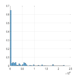
1. Original $T$

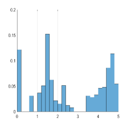
2. Box-Cox

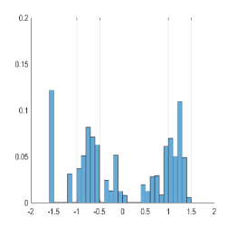
3. Box-Cox & Std.

In this figure we draw histograms of the treatment variable studied in Fong, Hazlett, and Imai (2018) (i.e. the number of political advertisements aired in each zip code). Panel 1 plots the original treatment $T$; Panel 2 plots $T^{\prime}$, namely the treatment after running the Box-Cox transformation with $\lambda=-0.16$; Panel 3 plots $T^{*}$, namely the standardized version of $T^{\prime}$. For each histogram, the sum of the heights of bars is normalized to 1 so that the vertical axis is associated with empirical probability.

References

- (1)
- Abadie, Angrist, and Imbens (1998) Abadie, A., J. D. Angrist, and G. W. Imbens (1998): “Instrumental Variables Estimation of Quantile Treatment Effects,” Nber Technical Working Papers.
- Ai, Linton, Motegi, and Zhang (2018) Ai, C., O. Linton, K. Motegi, and Z. Zhang (2018): “Supplemental material for ’A Unified Framework for Efficient Estimation of Binary, Multi-level, Continuous and Mixture of Discrete and Continuous Treatment Models with Estimated Stabilized Weights’,” Discussion paper, University of Florida.
- Andrews (1991) Andrews, D. W. (1991): “Asymptotic normality of series estimators for nonparametric and semiparametric regression models,” Econometrica: Journal of the Econometric Society, pp. 307–345.
- Andrews (1994) (1994): “Empirical process methods in econometrics,” Handbook of econometrics, 4, 2247–2294.
- Angrist and Pischke (2008) Angrist, J. D., and J.-S. Pischke (2008): Mostly harmless econometrics: An empiricist’s companion. Princeton university press.
- Bang and Robins (2005) Bang, H., and J. M. Robins (2005): “Doubly robust estimation in missing data and causal inference models,” Biometrics, 61(4), 962–973.
- Bickel, Klaassen, Ritov, and Wellner (1993) Bickel, P. J., C. A. J. Klaassen, Y. Ritov, and J. A. Wellner (1993): Efficient and Adaptive Estimation for Semiparametric Models. The Johns Hopkins University Press.
- Boneva, Elliot, Kaminska, Linton, Morely, and McLaren (2018) Boneva, L., D. Elliot, I. Kaminska, O. Linton, B. Morely, and N. McLaren (2018): “The Impact of QE on liquidity: Evidence from the UK Corporate Bond Purchase Scheme,” Bank of England working paper.
- Cao, Tsiatis, and Davidian (2009) Cao, W., A. A. Tsiatis, and M. Davidian (2009): “Improving efficiency and robustness of the doubly robust estimator for a population mean with incomplete data,” Biometrika, 96(3), 723–734.
- Cattaneo (2010) Cattaneo, M. D. (2010): “Efficient semiparametric estimation of multi-valued treatment effects under ignorability,” Journal of Econometrics, 155(2), 138–154.
- Chan, Yam, and Zhang (2016) Chan, K. C. G., S. C. P. Yam, and Z. Zhang (2016): “Globally efficient non-parametric inference of average treatment effects by empirical balancing calibration weighting,” Journal of the Royal Statistical Society: Series B (Statistical Methodology), 78(3), 673–700.
- Chen (2007) Chen, X. (2007): “Large sample sieve estimation of semi-nonparametric models,” Handbook of Econometrics, 6(B), 5549–5632.
- Chernozhukov, Fernández-Val, and Melly (2013) Chernozhukov, V., I. Fernández-Val, and B. Melly (2013): “Inference on counterfactual distributions,” Econometrica, 81(6), 2205–2268.
- Chernozhukov and Hansen (2010) Chernozhukov, V., and C. Hansen (2010): “An IV Model of Quantile Treatment Effects,” Econometrica, 73(1), 245–261.
- Doksum (1974) Doksum, K. (1974): “Empirical Probability Plots and Statistical Inference for Nonlinear Models in the Two-Sample Case,” Annals of Statistics, 2(2), 267–277.
- Donald and Hsu (2014) Donald, S. G., and Y. C. Hsu (2014): “Estimation and inference for distribution functions and quantile functions in treatment effect models ☆,” Journal of Econometrics, 178(1), 383–397.
- Fan and Park (2010) Fan, Y., and S. S. Park (2010): “Sharp bounds on the distribution of treatment effects and their statistical inference,” Econometric Theory, 26(3), 931–951.
- Firpo (2007) Firpo, S. (2007): “Efficient Semiparametric Estimation of Quantile Treatment Effects,” Econometrica, 75(1), 259–276.
- Florens, Heckman, Meghir, and Vytlacil (2008) Florens, J.-P., J. J. Heckman, C. Meghir, and E. Vytlacil (2008): “Identification of treatment effects using control functions in models with continuous, endogenous treatment and heterogeneous effects,” Econometrica, 76(5), 1191–1206.
- Fong, Hazlett, and Imai (2017) Fong, C., C. Hazlett, and K. Imai (2017): “Covariate balancing propensity score for a continuous treatment: Application to the efficacy of political advertisements,” forthcoming in the Annals of Applied Statistics.
- Fong, Hazlett, and Imai (2018) (2018): “Covariate Balancing Propensity Score for a Continuous Treatment: Application to the Efficacy of Political Advertisements,” Annals of Applied Statistics, 12(1), 156–177.
- Frölich and Melly (2013) Frölich, M., and B. Melly (2013): “Unconditional Quantile Treatment Effects Under Endogeneity,” Journal of Business and Economic Statistics, 31(3), 346–357.
- Graham, Pinto, and Egel (2012) Graham, B. S., C. C. D. X. Pinto, and D. Egel (2012): “Inverse probability tilting for moment condition models with missing data,” The Review of Economic Studies, 79(3), 1053–1079.
- Hahn (1998) Hahn, J. (1998): “On the role of the propensity score in efficient semiparametric estimation of average treatment effects,” Econometrica, 66(2), 315–331.
- Heckman and Vytlacil (2005) Heckman, J. J., and E. Vytlacil (2005): “Structural equations, treatment effects, and econometric policy evaluation,” Econometrica, 73(3), 669–738.
- Hirano and Imbens (2004) Hirano, K., and G. W. Imbens (2004): “The propensity score with continuous treatments,” in Applied Bayesian Modeling and Causal Inference from Incomplete-Data Perspectives, ed. by A. Gelman, and X.-L. Meng, chap. 7, pp. 73–84. John Wiley & Sons Ltd.
- Hirano, Imbens, and Ridder (2003) Hirano, K., G. W. Imbens, and G. Ridder (2003): “Efficient Estimation of Average Treatment Effects Using the Estimated Propensity Score,” Econometrica, 71(4), 1161–1189.
- Imai and van Dyk (2004) Imai, K., and D. A. van Dyk (2004): “Causal inference with general treatment regimes: Generalizing the propensity score,” Journal of the American Statistical Association, 99(467), 854–866.
- Imbens (2000) Imbens, G. W. (2000): “The role of the propensity score in estimating dose-response functions,” Biometrika, 87(3), 706–710.
- Imbens (2004) (2004): “Nonparametric estimation of average treatment effects under exogeneity: A review,” The review of Economics and Statistics, 86(1), 4–29.
- Imbens and Wooldridge (2009) Imbens, G. W., and J. M. Wooldridge (2009): “Recent developments in the econometrics of program evaluation,” Journal of Economic Literature, 47(1), 5–86.
- Kennedy, Ma, McHugh, and Small (2017) Kennedy, E. H., Z. Ma, M. D. McHugh, and D. S. Small (2017): “Non-parametric methods for doubly robust estimation of continuous treatment effects,” Journal of the Royal Statistical Society: Series B (Statistical Methodology), 79(4), 1229–1245.
- Lehmann (1974) Lehmann, E. (1974): Nonparametrics: Statistical Methods Based on Ranks.
- Masry (1996) Masry, E. (1996): “Multivariate local polynomial regression for time series: uniform strong consistency and rates,” Journal of Time Series Analysis, 17(6), 571–599.
- Newey (1994) Newey, W. K. (1994): “The Asymptotic Variance of Semiparametric Estimators,” Econometrica, 62(6), 1349–1382.
- Newey (1997) (1997): “Convergence Rates and Asymptotic Normality for Series Estimators,” Journal of Econometrics, 79(1), 147–168.
- Newey and Powell (1987) Newey, W. K., and J. L. Powell (1987): “Asymmetric least squares estimation and testing,” Econometrica: Journal of the Econometric Society, pp. 819–847.
- Qin and Zhang (2007) Qin, J., and B. Zhang (2007): “Empirical-likelihood-based inference in missing response problems and its application in observational studies,” Journal of the Royal Statistical Society: Series B (Statistical Methodology), 69(1), 101–122.
- Robins, Hernán, and Brumback (2000) Robins, J. M., M. A. Hernán, and B. Brumback (2000): “Marginal structural models and causal inference in epidemiology,” Epidemiology, 11(5), 550–560.
- Robins, Rotnitzky, and Zhao (1994) Robins, J. M., A. Rotnitzky, and L. P. Zhao (1994): “Estimation of regression coefficients when some regressors are not always observed,” Journal of the American Statistical Association, 89(427), 846–866.
- Rosenbaum and Rubin (1983) Rosenbaum, P. R., and D. B. Rubin (1983): “The central role of the propensity score in observational studies for causal effects,” Biometrika, 70(1), 41–55.
- Rothe (2017) Rothe, C. (2017): “Robust confidence intervals for average treatment effects under limited overlap,” Econometrica, 85(2), 645–660.
- Słoczyński and Wooldridge (2017) Słoczyński, T., and J. M. Wooldridge (2017): “A general double robustness result for estimating average treatment effects,” Econometric Theory, pp. 1–22.
- Tan (2010) Tan, Z. (2010): “Bounded, efficient and doubly robust estimation with inverse weighting,” Biometrika, 97(3), 661–682.
- Tseng and Bertsekas (1991) Tseng, P., and D. P. Bertsekas (1991): “Relaxation methods for problems with strictly convex costs and linear constraints,” Mathematics of Operations Research, 16(3), 462–481.
- Urban and Niebler (2014) Urban, C., and S. Niebler (2014): “Dollars on the Sidewalk: Should U.S. Presidential Candidates Advertise in Uncontested States?,” American Journal of Political Science, 58(2), 322–336.
- Vansteelandt, Bekaert, and Claeskens (2010) Vansteelandt, S., M. Bekaert, and G. Claeskens (2010): “On model selection and model misspecification in causal inference,” Statistical Methods in Medical Research, 21(1), 7–30.
- Yiu and Su (2018) Yiu, S., and L. Su (2018): “Covariate association eliminating weights: a unified weighting framework for causal effect estimation,” Biometrika.