Dynamical multistability in a quantum dot laser

Abstract

We study the dynamical multistability of a solid-state single-atom laser implemented in a quantum dot spin valve. The system is formed by a resonator that interacts with a two-level system in a dot in contact with two ferromagnetic leads of antiparallel polarization. We show that a spin-polarized current provides high-efficiency pumping leading to regimes of multistable lasing, in which the Fock distribution of the oscillator displays a multi-peaked distribution. The emergence of multistable lasing follows from the breakdown of the usual rotating-wave approximation for the coherent spin-resonator interaction which occurs at relatively weak couplings. The multistability manifests itself directly in the charge current flowing through the dot, switching between distinct current levels corresponding to the different states of oscillation.

I Introduction

Quantum conductors coupled to localized harmonic resonators, such as microwave photon cavities Liu et al. (2015); Mi et al. (2016); Viennot et al. (2015); Stockklauser et al. (2015, 2017); Li et al. (2018) or mechanical resonators Naik et al. (2006); Benyamini et al. (2014); Okazaki et al. (2016); Deng et al. (2016) have become commonly studied systems. They open the route to explore correlations between charge transport and emitted radiation Lambert et al. (2015) or induced mechanical vibrations Parafilo et al. (2016). Ultimately, these systems can encode single-atom lasers which exhibit unique features compared to conventional lasers such as absence of threshold, self-quenching, and sub-Poissonian statistics Filipowicz et al. (1986); Lugiato et al. (1987); Mu and Savage (1992); Rice and Carmichael (1994); Wang and Vyas (1996). Lasers where a cavity mode interacts with a stream of excited atoms one at a time Filipowicz et al. (1986); Lugiato et al. (1987) can display multistability Walther et al. (2006), whereby two or more stable amplitudes of oscillation coexist. Such behavior has also been predicted to occur in solid-state analogues, such as single-electron transistors Doiron et al. (2006); Rodrigues et al. (2007a, b); Micchi et al. (2015) and optomechanical systems Marquardt et al. (2006); Nation (2013).

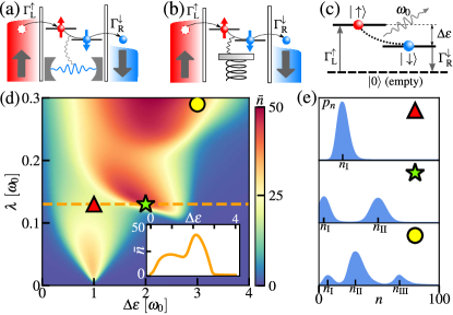
Figure 1: Model of a quantum-dot spin valve: (a) photon microwave cavity or (b) nanomechanical resonator interacting with two spin levels of energy difference $\Delta\varepsilon$. Electron tunneling occurs at rates $\Gamma^{\uparrow}_{\mathrm{L}}$ and $\Gamma^{\downarrow}_{\mathrm{R}}$ through ferromagnetic leads. (c) Energy diagram of the corresponding single-atom laser. (d) Average occupation of oscillator $\bar{n}$ as a function of spin energy splitting $\Delta\varepsilon$ and the spin-oscillator coupling strength $\lambda$ for fully polarized leads and $\Gamma^{\uparrow}_{\mathrm{L}}=\Gamma^{\downarrow}_{\mathrm{R}}=0.1\omega_{0}$, $Q=10^{3}$ (inset: line at $\lambda=0.13\omega_{0}$). (e) Steady-state Fock distributions $p_{n}$ at three different points (triangle, star and circle) marked in (d), with maxima at $n_{\mathrm{I}},n_{\mathrm{II}}$ and $n_{\mathrm{III}}$.

Single-atom lasers have been realized in cavity quantum electrodynamics (QED) McKeever et al. (2003); Walther et al. (2006), in circuit QED Astafiev et al. (2007) and in hybrid systems with double quantum dots coupled to microwave cavities Liu et al. (2017). Quantum dots are natural candidates for exploring the rich physics of single-atom lasing, given their tunability and versatility Childress et al. (2004); Jin et al. (2011); Liu et al. (2014, 2015); Brandes and Lambert (2003); Bergenfeldt and Samuelsson (2013). Theoretical works analyzed the possibility of lasing in open quantum dots Childress et al. (2004); Jin et al. (2011) and a number of successful experiments Liu et al. (2014); Gullans et al. (2015); Liu et al. (2015, 2017) reported lasing in double-quantum-dot systems. A single-atom laser using spin-polarized current in spin-valve quantum dots has also been proposed Khaetskii et al. (2013).

In this work, we show that a spin-valve quantum dot laser can display a rich range of multistable dynamics. The emergence of multistability turns out to be closely linked to the breakdown of the rotating-wave approximation (RWA), even though it occurs for relatively weak dot-oscillator couplings. This is in contrast to well-studied quantum optical systems which also display multistability, such as the micromaser Walther et al. (2006); Scully and Zubairy (1997). The spin-valve system therefore provides a very promising platform, not just for studying unconventional laser-like dynamics in hybrid systems, but also for investigating coherent spin-oscillator interactions beyond the RWA without the requirement for ultrastrong couplings Forn-Díaz et al. ; Kockum et al. (2019). The spin-oscillator model we consider is depicted in Figs. 1(a)-1(c); it comprises two levels of an electron spin with energy difference $\Delta\varepsilon$ within a quantum dot embedded between ferromagnetic contacts of opposite polarization. The spin interacts with a local resonator of frequency $\omega_{0}$ which can be a microwave photon cavity, Fig. 1(a), or a mechanical mode, Fig. 1(b). Assuming strong Coulomb repulsion forbids double occupation in the dot, the spin levels behave as a spin-$1/2$ interacting with the oscillator with coupling strength $\lambda$. For a single resonator mode with large quality factor and negligible relaxation rates for other (non-emitting) decay channels, lasing is achieved, as illustrated in Fig. 1(d), as a function of $\Delta\varepsilon$ and $\lambda$. Remarkably, regimes of bi- and multistability are readily found where two or more states of large amplitude of oscillation coexist, leading to corresponding maxima in the Fock distribution of the resonator, as illustrated in Fig. 1(e). We show that bistability can be achieved with experimentally accessible parameters and detected using simple measurements of the average current flowing through the dot.

This paper is organized as follows. In Sec. II, we introduce the model Hamiltonian and the master-equation formalism. Section III describes the single-atom laser properties of the model within the RWA, while in Sec. IV, we show how multistability emerges beyond the RWA. In Sec. V, we prove how the multistable dynamics can be detected through current measurements, while Sec. VI is devoted to the experimental feasibility study of the system. Finally, we draw our conclusions in Sec. VII.

II Model Hamiltonian and Master Equation

The dot-resonator system is described by the Rabi model Hamiltonian $(\hbar=1)$

$$\hat{H}=\frac{\Delta\varepsilon}{2}\hat{\sigma}_{z}+\omega_{0}\hat{b}^{\dagger}\hat{b}+\lambda(\hat{\sigma}_{+}+\hat{\sigma}_{-})(\hat{b}+\hat{b}^{\dagger}),$$ (1)

with $\hat{b},\hat{b}^{\dagger}$ the annihilation and creation operators of the oscillator, $\hat{\sigma}_{\pm}=(\hat{\sigma}_{x}\pm i\hat{\sigma}_{y})/2$ and $\hat{\sigma}_{x},\hat{\sigma}_{y},\hat{\sigma}_{z}$ Pauli spin operators associated to the two spin levels of the dot, polarized in the $z$-direction, and with a transverse interaction with the oscillator via $\hat{\sigma}_{x}$.

In the limiting case of fully spin-polarized leads, the left contact fills the spin-up level whereas spin-down electrons escape to the right, see Fig. 1. The coherent interaction with the oscillator provides a spin-flipping mechanism allowing an (inelastic) current to flow through the dot accompanied by energy release into the oscillator: each electron passing through the dot emits one quantum of oscillation. However, the perfect correspondence between creation of quanta and flow of current is broken if there is intrinsic spin relaxation in the dot, or if the polarization in the leads is incomplete (so electrons can tunnel in and out from both spin levels). When the lead polarizations are $P_{\nu}$, with $\nu={\mathrm{L}},{\mathrm{R}}$, the spin-dependent tunneling rates are given by $\Gamma_{\nu}^{\sigma}=\Gamma_{\nu}(1+\sigma P_{\nu})/2$ for spin index $\sigma=\uparrow/\downarrow=+/-$. For simplicity, we assume throughout symmetric and opposite polarization, i.e., $P_{\mathrm{R}}=-P_{\mathrm{L}}=P$, with $0<P\leq 1$.

We focus on the regime $\Gamma_{\nu}^{\sigma}\ll eV$, with $V$ the bias voltage and $e$ the electron charge. Notice that the strong coupling limit is not necessary in our model since we can have $\lambda\ll\Gamma_{\nu}^{\sigma}$. For large bias voltage the average energy of the two spin levels is well inside the bias window, and transport from right to left is blocked. In this regime the dynamics is captured by a Markovian master equation in Lindblad form for the density matrix $\hat{\rho}$ of the coupled dot-resonator system Breuer and Petruccione (2002); Timm (2008); Cohen-Tannoudji et al. (1992). Tracing out the leads, and assuming local dissipation within each subsystem (dot and oscillator), the master equation at zero-temperature reads

$$\dot{\hat{\rho}}=-i[\hat{H},\hat{\rho}]+\!\!\!\!\sum_{\sigma=\uparrow,\downarrow}\ [\Gamma^{\sigma}_{\mathrm{L}}\mathcal{D}(\hat{F}^{\dagger}_{\sigma})\hat{\rho}+\Gamma^{\sigma}_{\mathrm{R}}\mathcal{D}(\hat{F}_{\sigma})\hat{\rho}]+\kappa\mathcal{D}(\hat{b})\hat{\rho},$$ (2)

where $\kappa$ is the oscillator damping rate (related to the quality factor by $Q=\omega_{0}/\kappa$). We have denoted the Lindblad dissipator with $\mathcal{D}(\hat{x})\hat{\rho}=\hat{x}\hat{\rho}\hat{x}^{\dagger}-(\hat{x}^{\dagger}\hat{x}\hat{\rho}+\hat{\rho}\hat{x}^{\dagger}\hat{x})/2$. The operators $\hat{F}_{\sigma}=(1-\hat{n}_{-{\sigma}})\hat{d}_{\sigma}$ and $F^{\dagger}_{\sigma}$ describe incoherent electron tunneling with the constraint of vanishing double occupation. $\hat{d}_{\sigma}$ is the fermionic operator which annihilates an electron of spin $\sigma$ in the dot and $\hat{n}_{\sigma}$ is the corresponding number operator. The mappings $\hat{\sigma}_{z}=\hat{n}_{\uparrow}-\hat{n}_{\downarrow}$ and $\hat{\sigma}_{x}=\hat{d}^{\dagger}_{\uparrow}\hat{d}_{\downarrow}+\hat{d}^{\dagger}_{\downarrow}\hat{d}_{\uparrow}$ hold in Hamiltonian (1). The derivation of Eq. (2) is given in Appendix A. The steady-state solution of Eq. (2) is found numerically using the Python package QuTiP Johansson et al. (2012, 2013).

III Standard single-atom laser and RWA

For weak spin-oscillator coupling, the rotating-wave approximation (RWA) is expected to be valid and $\hat{H}$ is approximated by

$$\hat{H}^{\mathrm{RWA}}=\frac{\Delta\varepsilon}{2}\hat{\sigma}_{z}+\omega_{0}\hat{b}^{\dagger}\hat{b}+\lambda(\hat{\sigma}_{+}\hat{b}+\hat{\sigma}_{-}\hat{b}^{\dagger}).$$ (3)

Using Eq. (3) in Eq. (2) we recover well-known approximate analytical solutions for the oscillator Fock probability distribution $p_{n}$ of a three-level single-atom laser Scully and Zubairy (1997), see Appendix B.1. The average Fock number $\bar{n}=\langle\hat{b}^{\dagger}\hat{b}\rangle$ calculated numerically coincides with the analytical results in Fig. 2(a): incoherent pumping by electron tunneling establishes a spin population inversion leading to lasing.

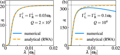
Figure 2: Average occupation $\bar{n}$ of the oscillator as a function of $\lambda$, for fully polarized leads at $\Delta\varepsilon=\omega_{0}$. Solid lines are numerical calculations, dashed lines are the analytical results from the Fock distribution $p_{n}$ obtained within the RWA. The vertical and horizontal dotted lines are the threshold $\lambda_{\mathrm{thr}}$ and saturation number $A_{s}^{2}$, respectively, predicted by the semiclassical equations in RWA.

By combining the RWA with a semiclassical approximation Mu and Savage (1992), the operator $\hat{b}$ is replaced by its time-dependent, classical expectation value $\alpha(t)$, assuming quantum fluctuations are negligible (viz., above the lasing threshold). The spin is still described quantum mechanically by a density matrix with $\rho_{\uparrow}(t)$ and $\rho_{\downarrow}(t)$ the diagonal elements and $\rho_{\uparrow\downarrow}(t)$ the off-diagonal element. The dot occupation probability is $p_{1}=\rho_{\uparrow}+\rho_{\downarrow}$ whereas $S_{z}=\rho_{\uparrow}-\rho_{\downarrow}$ is the spin polarization. Moving to a rotating frame with $\alpha(t)\rightarrow\tilde{\alpha}(t)e^{-i\omega_{0}t},\rho_{\uparrow\downarrow}(t)\rightarrow\tilde{\rho}_{\uparrow\downarrow}(t)e^{-i\Delta\varepsilon t}$, we obtain a set of nonlinear equations for $\tilde{\alpha}(t)$, $p_{1}(t)$ and the spin vector $\vec{S}(t)=[S_{x}(t),S_{y}(t),S_{z}(t)]^{T}$ with $\tilde{\rho}_{\uparrow\downarrow}(t)=[S_{x}(t)-iS_{y}(t)]/2$, derived in Appendix B.2. Within this framework, lasing is equivalent to self-sustained oscillations: the relaxation dynamics for the amplitude $\left|\tilde{\alpha}\right|=A$ is given by

$$\dot{A}=-[\kappa+\gamma_{\mathrm{rw}}(A)]\frac{A}{2}$$ (4)

with the effective, negative nonlinear damping

$$\gamma_{\mathrm{rw}}(A)=-\frac{\lambda^{2}\Gamma_{\mathrm{eff}}}{\lambda^{2}A^{2}+\Gamma_{\mathrm{eff}}\Gamma^{\downarrow}_{\mathrm{R}}/4}$$ (5)

where $\Gamma_{\mathrm{eff}}=\Gamma^{\uparrow}_{\mathrm{L}}\Gamma^{\downarrow}_{\mathrm{R}}/(2\Gamma^{\uparrow}_{\mathrm{L}}+\Gamma^{\downarrow}_{\mathrm{R}})$. Equation (4) predicts a stable steady-state solution of finite $A$ above a threshold coupling $\lambda_{\mathrm{thr}}$. For fully polarized leads ($P=1$) and on resonance ($\Delta\varepsilon=\omega_{0}$), one obtains $\lambda_{\mathrm{thr}}^{2}=\Gamma^{\downarrow}_{\mathrm{R}}\omega_{0}/(4Q)$ and for $\lambda\gg\lambda_{\mathrm{thr}}$ the amplitude saturates to $A_{s}=\sqrt{\Gamma_{\mathrm{eff}}Q/\omega_{0}}$. Semiclassical predictions for the saturation and threshold are shown as straight lines in Fig. 2.

We conclude by observing that, for finite polarization, we have the weak scaling $\lambda_{\mathrm{thr}}\sim 1/\sqrt{P}$, $A_{s}\sim\sqrt{P}$, as shown in Appendix B.

IV Multistability beyond RWA

The RWA predicts that the saturation amplitude $A_{s}$ should simply increase with increasing $Q$ and $\Gamma_{\mathrm{eff}}$, without any other changes developing. However, numerical calculations show that the average Fock occupation ($\bar{n}$) no longer saturates and instead drops with increasing $\lambda$, see Fig. 2(b). This breakdown in the RWA occurs when the Rabi oscillation frequency of the spin (which is proportional to $\lambda A$) approaches $\omega_{0}$. In fact, for large enough Rabi frequencies, the Fock distribution (obtained numerically) becomes multi-peaked with the highest peak close to the amplitude predicted by the RWA, Fig. 1(e). This happens even at finite detuning ($\Delta\varepsilon\neq\omega_{0}$) giving rise to the complex behavior of $\bar{n}$ reported in Fig. 1(d). By extending the semiclassical approach to analyze the behavior beyond RWA, we show that the oscillator dynamics can possess two or more coexisting stable limit cycles with different amplitudes. The resulting phase diagram of the bi- and multistable regions agrees closely with the numerical results as shown in Figs. 3(b) and 3(c).

Focusing on the case $\Gamma^{\uparrow}_{\mathrm{L}}=\Gamma^{\downarrow}_{\mathrm{R}}/2=\Gamma$ to simplify the discussion, $p_{1}$ becomes irrelevant and we write again a set of nonlinear equations for $\tilde{\alpha}(t)$ and $\vec{S}(t)$ in the rotating frame (see Appendix C for details). In the regime $\kappa\ll\lambda,\Gamma,\omega_{0}$, the oscillator amplitude $|\tilde{\alpha}|=A$ is a slow variable while its phase is irrelevant and can be set to zero. Assuming constant $A$, the equation for the spin vector when $\Delta\varepsilon=\omega_{0}$ and $P=1$ is

$$\dot{\vec{S}}(t)=\Gamma\hat{u}_{z}-\Gamma\vec{S}(t)+\vec{S}(t)\times\vec{B}(t),$$ (6)

with $\hat{u}_{z}$ unit vector in the $z$-direction and

$$\vec{B}(t)=\left(\begin{array}[]{c}B_{x}(t)\\ B_{y}(t)\end{array}\right)=2\lambda A\left(\begin{array}[]{c}-1-\cos(2\omega_{0}t)\\ \sin(2\omega_{0}t)\end{array}\right).$$ (11)

The behavior of the solutions of Eqs. (6)-(11) is similar to that seen in previous studies on circuit-QED systems Rodrigues et al. (2007b) and is related to a phase-locking phenomenon in which the Rabi frequency of the spin—determined by the oscillation amplitude—seeks to be commensurate to the oscillator frequency Marquardt et al. (2006). By writing Eq. (6) in Fourier space, with $S_{k}(t)=\sum_{n}S_{k}^{(n)}e^{2in\omega_{0}t},\ (k=x,y,z),$ we obtain a recursion relation for the $A$-dependent Fourier coefficient $S_{z}^{(n)}$ in terms of $S_{z}^{(n\pm 1)}$. We can then calculate the amplitude-dependent effective negative nonlinear damping $\gamma_{\mathrm{eff}}$ acting on the oscillator due to the spin dynamics,

$$\gamma_{\mathrm{eff}}(A)=-\frac{2\lambda^{2}}{\Gamma}\left[\frac{4\omega_{0}^{2}}{\Gamma^{2}+4\omega_{0}^{2}}S_{z}^{(0)}-\mathrm{Im}\left(\frac{2\omega_{0}}{\Gamma+2i\omega_{0}}S_{z}^{(1)}\right)\right].$$ (12)

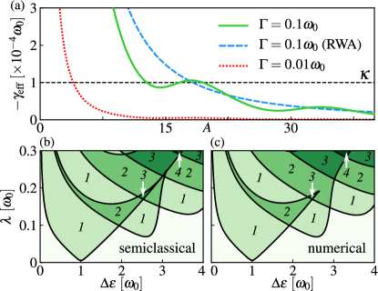
Figure 3: (a) Effective negative nonlinear damping $\gamma_{\mathrm{eff}}(A)$ for the oscillator, as given by Eq. (12) on resonance $\Delta\varepsilon=\omega_{0}$ and for $\lambda=0.055\omega_{0}$. Intersections with the horizontal dashed line at $\kappa=10^{-4}\omega_{0}$ indicate limit cycles for the amplitude. (b) Multistability diagram obtained with the semiclassical approximation, showing the number of stable limit cycles (italic numbers) as a function of $\Delta\varepsilon$ and $\lambda$. (c) Multistability diagram obtained from the numerical solution of the Lindblad equation (number of peaks in the Fock distribution). Parameters: $Q=10^{3},\ P=1,\ \Gamma=0.05\omega_{0}$.

We show the results for $\gamma_{\mathrm{eff}}$ on resonance in Fig. 3(a). The monotonic RWA behavior $\gamma_{\mathrm{eff}}\approx\gamma_{\mathrm{rw}}$ is recovered only at low tunneling rate whereas the function $\gamma_{\mathrm{eff}}$ oscillates at larger $\Gamma$ with maxima close to the points $\lambda A\sim j\omega_{0}$ with $j$ integer. This nonmonotonic behavior leads to many (stable) limit cycles determined by the intersections $\kappa=-\gamma_{\mathrm{eff}}(A)$ with a negative slope of $|\gamma_{\mathrm{eff}}(A)|$. Equation (12) is readily generalized to the off-resonant case in Appendix C.2 and we can extract the stable steady-state amplitudes to produce the predicted multistability diagram, Fig. 3(b). We test the validity of the semiclassical solution by finding numerically the steady-state Fock distribution $p_{n}$ of the system through Eq. (2) and computing the number of distinct peaks in $p_{n}$ with $n>0$, see Fig. 3(c).

The semiclassical method has the important advantage that it can be used to calculate the onset of bi- and multistability at relatively weak coupling strengths, $\lambda\sim 10^{-3}\omega_{0}$, and high quality factors, $Q\sim 10^{5}$, which are most likely to be accessible experimentally (as discussed below). For large $Q$, the average occupation number is too large to allow a full numerical solution of the master equation, since it requires a prohibitively large cutoff in the Fock state basis.

V Current jumps

Measurement of the dc-current through the dot provides a simple way to detect lasing and bistability. In the large bias limit the current is given by

$$I=e(\Gamma_{\mathrm{R}}^{\uparrow}\rho_{\uparrow}+\Gamma_{\mathrm{R}}^{\downarrow}\rho_{\downarrow}).$$ (13)

In the fully polarized case the total current is purely inelastic (oscillator-assisted spin flips), $I=e\Gamma_{\mathrm{R}}^{\downarrow}\rho_{\downarrow}$, and on resonance we have $\kappa\bar{n}=I/e$, as expected by energy conservation: the outgoing flux of quanta equals the ingoing flux of energy into the oscillator. For large oscillator occupation number (i.e., large oscillation amplitudes in the semiclassical framework), the average current is much larger than its fluctuations and acts as a measure of the oscillator amplitude as illustrated in Fig. 4(a).

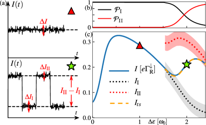
Figure 4: (a) Sketch of the behavior of the current in the lasing regime with a single stable oscillator amplitude $A_{\mathrm{I}}$ (upper) and in a bistable regime with distinct stable amplitudes $A_{\mathrm{I}}$ and $A_{\mathrm{II}}$ (lower). (b) Occupation probabilities $\mathcal{P}_{\mathrm{I}}$ and $\mathcal{P}_{\mathrm{II}}$ of the two states computed numerically. (c) Average current computed numerically (solid blue line) and using the effective two-state model (dashed orange line). The upper (red) and lower (black) dotted lines show the two current states $I_{\mathrm{I}}$ and $I_{\mathrm{II}}$ along with their variance, represented by the shaded areas. The parameters match those of the inset in Fig. 1(d).

The current also provides a simple way to detect the RWA breakdown and the onset of bistable regime, as it can display telegraph dynamics. For a well-developed bistability, the oscillator exists in a mixed state containing two different limit cycles with well-separated amplitudes $A_{\mathrm{I}}$ and $A_{\mathrm{II}}$ and associated probabilities $\mathcal{P}_{\mathrm{I}}$ and $\mathcal{P}_{\mathrm{II}}$. The amplitude is then expected to switch randomly between two well-defined plateaus when $\mathcal{P}_{\mathrm{I}}\sim\mathcal{P}_{\mathrm{II}}$. The close connection between current and oscillator amplitude suggests that the telegraph dynamics will manifest itself in random switching between plateaus of different average current associated with the different states of oscillation Kirton and Armour (2013), as sketched in Fig. 4(a). Such behavior is also naturally implied by the semiclassical treatment in which, for each stable amplitude solution $A_{\mathrm{I}},A_{\mathrm{II}}$ of the oscillator, one has a different solution for the average current, $I_{\mathrm{I}}$ and $I_{\mathrm{II}}$.

Telegraph behavior of the current should be observable if: (i) $\mathcal{P}_{\mathrm{I}}\sim\mathcal{P}_{\mathrm{II}}$; (ii) the variance associated to each plateau is smaller than the distance: $\Delta I_{\mathrm{I}},\Delta I_{\mathrm{II}}\ll|I_{\mathrm{I}}-I_{\mathrm{II}}|$; (iii) the lifetime of each plateau is sufficiently long to observe separated jumps. Under these conditions the system is well described by an effective two-state model with transition rates $W_{\mathrm{I}\rightarrow\mathrm{II}}$ and $W_{\mathrm{II}\rightarrow\mathrm{I}}$. We test the appropriateness of the two-state model by computing the probabilities $\mathcal{P}_{\mathrm{I}}$, $\mathcal{P}_{\mathrm{II}}$ (from the areas of the two peaks in the $p_{n}$ distribution) and by comparing the average dc-current calculated numerically with the two-state expression

$$I_{ts}=\mathcal{P}_{\mathrm{I}}I_{\mathrm{I}}+\mathcal{P}_{\mathrm{II}}I_{\mathrm{II}},$$ (14)

see Fig. 4(b,c). Here we also report the current variance for each plateau $\Delta I_{\mathrm{I}}$ and $\Delta I_{\mathrm{II}}$ defined as $\Delta I_{\mathrm{I}}=\sqrt{\Gamma S_{\mathrm{I}}}$ and $\Delta I_{\mathrm{II}}=\sqrt{\Gamma S_{\mathrm{II}}}$, with $S_{\mathrm{I}}$, $S_{\mathrm{II}}$ the current shot-noise. Finally, we obtain the sum of the two rates $W_{\mathrm{I}\rightarrow\mathrm{II}}+W_{\mathrm{II}\rightarrow\mathrm{I}}$ by comparing the current shot-noise, calculated numerically with the full counting statistics method, to the two-state formula (see Appendices D-E and Refs. Flindt et al., 2004, 2005, 2010; Usmani et al., 2007; Brüggemann et al., 2012 for details). This sum agrees well with the real part of the smallest nonzero eigenvalue of the system Liouvillian, verifying the applicability of the two-state model and showing that the switching can be extremely slow (orders of magnitude slower than the relaxation time of the oscillator) Harvey et al. (2008) as discussed in Appendix E.

VI Experimental feasibility

At finite polarization the total current has an elastic contribution in addition to the inelastic one that arises from the interaction with the oscillator. This leads to lower efficiency, but lasing and multistability are still achievable. Importantly, the inelastic current is still a substantial fraction of the total current (larger than the noise) such that the current jumps are still clearly observable. Using numerical calculations, we test that the results presented so far are robust against effects of finite polarization. Having in mind the case of mechanical oscillators, we also include the effects of finite temperature $T$ (namely, $n_{\mathrm{B}}>0$ with $n_{\mathrm{B}}=[\exp(\omega_{0}/T)-1]^{-1}$ the thermal bosonic occupation number and $k_{\mathrm{B}}=1$) and intrinsic nonlinearity Meerwaldt et al. (2012). The multistability is preserved in a substantial range of parameters far from the ideal case (e.g., $P=0.5$) including finite internal spin relaxation of the dot, which plays a role similar to finite polarization: impinging spin-up electrons can decay into the spin-down level and pass through the dot without quanta emission. When the spin relaxation rate $\gamma_{\mathrm{sr}}$ is smaller than the tunneling rates $\Gamma$ and the Rabi frequency $\lambda A$, lasing and multistability remain unperturbed. Several examples of the behaviour of the results including finite temperature, finite polarization, spin relaxation and Duffing nonlinearity are shown in Appendix F.

Spin-valve-based carbon nanotube quantum dots (CNTQDs) provide a promising way of implementing the model system we have investigated. CNTQDs can achieve high spin polarization of injected electrons Sahoo et al. (2005) and small spin relaxation rate Rice et al. (2013); Churchill et al. (2009); Viennot et al. (2015). Furthermore, suspended nanotubes act as electromechanical systems with vibrational modes of huge quality factor Moser et al. (2014). Spin-vibration interaction in suspended CNTQDs has been investigated theoretically in spin-valve setups Pályi et al. (2012); Stadler et al. (2014, 2015). For $Q=10^{6}$, $P=0.5$, $\Gamma_{\mathrm{L}}=\Gamma_{\mathrm{R}}=0.05\omega_{0}$, we estimate a threshold $\lambda_{\mathrm{thr}}\approx 1.6\times 10^{-4}\omega_{0}$ which is well below the expected interaction strength $\lambda\approx 1\ \text{MHz}$ for a typical resonance frequency $\omega_{0}/2\pi=100\ \text{MHz}$ Stadler et al. (2014, 2015).

Realizations based on spin valves coupled to microwave cavities should also be possible. Reliable coupling of CNTQDs with superconducting microwave cavities has been demonstrated Ranjan et al. (2015). Spin-photon interactions have also been implemented in quantum dots with ferromagnetic leads Viennot et al. (2015) and, more recently, in silicon double dots embedded in magnetic nanostructures Mi et al. (2018).

VII Conclusions

We have analyzed a model quantum dot spin valve which forms an unconventional single-atom laser: a spin-polarized current pumps the motion of a resonator coupled to the dot very efficiently, allowing access to novel regimes of multistable lasing. We show that multistability develops when the dot-resonator interaction is no longer captured by the conventional RWA—which is expected to occur for the relatively weak couplings achievable with current devices—because large amplitude motion of the resonator enhances the effective coupling strength. This type of system provides an alternative route for investigating coherent dynamics beyond the RWA without the need for ultrastrong couplings. Our work raises a range of interesting questions about the extent to which the multistable lasing dynamics can be controlled and exploited, e.g., in nonlinear amplifiers or force sensing devices.

Appendix A Derivation of the master equation

In this Appendix we derive Eq. (2) and discuss critically its validity regime. We start from the model Hamiltonian that describes a quantum dot with spin-dependent levels, between two lateral leads, and coupled to an harmonic oscillator damped through a bosonic thermal bath ($\hbar=1$):

$$\hat{H}_{\mathrm{tot}} =\hat{H}+\hat{H}_{\mathrm{leads}}+\hat{H}_{\mathrm{tun}}+\hat{H}_{\mathrm{bath}}+\hat{H}_{\mathrm{osc-bath}},$$ (15)

with

$$\hat{H} =\varepsilon_{0}(\hat{n}_{\uparrow}+\hat{n}_{\downarrow})+\frac{\Delta\varepsilon}{2}(\hat{n}_{\uparrow}-\hat{n}_{\downarrow})+U\hat{n}_{\uparrow}\hat{n}_{\downarrow}$$

$$\,\,+\omega_{0}\hat{b}^{\dagger}\hat{b}+\lambda(\hat{d}^{\dagger}_{\uparrow}\hat{d}_{\downarrow}+\hat{d}^{\dagger}_{\downarrow}\hat{d}_{\uparrow})(\hat{b}+\hat{b}^{\dagger}),$$ (16)

$$\hat{H}_{\mathrm{leads}} =\sum_{\nu=\mathrm{L\,,R}}\sum_{k\sigma}(\epsilon_{\nu k\sigma}-\mu_{\nu})\hat{c}^{\dagger}_{\nu k\sigma}\hat{c}_{\nu k\sigma}^{\phantom{g}},$$ (17)

$$\hat{H}_{\mathrm{tun}} =\sum_{\nu=\mathrm{L\,,R}}\sum_{k\sigma}V_{\nu\sigma}\left(\hat{c}_{\nu k\sigma}^{\phantom{g}}\hat{d}^{\dagger}_{\sigma}+\mathrm{H.c.}\right),$$ (18)

$$\hat{H}_{\mathrm{osc-bath}} =\hat{b}\hat{B}+\mathrm{H.c.}$$ (19)

We have labeled with $\varepsilon_{0}$ the average energy of the two levels in the dot and $\Delta\varepsilon$ their energy separation. The Coulomb interaction is taken into account via the repulsive energy $U>0$ for the doubly-occupied state. $\hat{H}_{\mathrm{leads}}$ corresponds to the leads, viz., two Fermi gases, with $\hat{c}_{\nu k\sigma}$ the annihilation operator for a level of energy $\epsilon_{\nu k\sigma}$ on the $\nu$ lead kept at chemical potential $\mu_{\nu}$. The coupling between the leads and the dot is realized through the tunneling Hamiltonian $\hat{H}_{\mathrm{tun}}$, with $V_{\nu\sigma}$ the tunneling amplitudes. Finally, the oscillator is linearly coupled to a bosonic bath (described by $\hat{H}_{\mathrm{bath}}$) through the operator of the bath $\hat{B}$.

A.1 Born-Markov master equation

We identify our system as the dot coupled to the oscillator, evolving coherently under Hamiltonian (16), and we seek for the Markovian master equation describing the evolution of the system density matrix $\hat{\rho}$, using the standard open systems approach Breuer and Petruccione (2002); Cohen-Tannoudji et al. (1992). The external environment is described by $\hat{H}_{E}=\hat{H}_{\mathrm{leads}}+\hat{H}_{\mathrm{bath}}$, interacting with the system through $\hat{H}_{\mathrm{int}}=\hat{H}_{\mathrm{tun}}+\hat{H}_{\mathrm{osc-bath}}$. In the interaction picture with respect to $\hat{H}+\hat{H}_{E}$, the exact equation for the total density matrix $\hat{\rho}_{\mathrm{tot}}$ is

$$\dot{\hat{\rho}}_{\mathrm{tot},I}(t)= -i\left[\hat{H}_{\mathrm{int},I}(t),\hat{\rho}_{\mathrm{tot},I}(t_{0})\right]$$

$$-\int_{t_{0}}^{t}\!\!\!\!\mathrm{d}t^{\prime}\,\,\left[\hat{H}_{\mathrm{int},I}(t),\left[\hat{H}_{\mathrm{int},I}(t^{\prime}),\hat{\rho}_{\mathrm{tot},I}(t^{\prime})\right]\right],$$ (20)

where the subscript $I$ refers to the interaction picture. At this point, a number of assumptions are in order. (i) We assume that the interaction with the leads and the bath is turned on at some initial time $t_{0}$. Up to this instant, the total density matrix is factorized, $\hat{\rho}_{\mathrm{tot}}(t_{0})=\hat{\rho}(t_{0})\hat{\rho}_{\mathrm{leads}}(t_{0})\hat{\rho}_{\mathrm{bath}}(t_{0})$ (the tensor product is implied); the reservoirs are at separate thermal equilibria (the leads can have different chemical potentials). (ii) The internal correlations in the environments decay on a timescale which is much shorter than the timescale of interaction between the dot and the leads (given in the interaction picture by the inverse of the average tunneling amplitude $\overline{V_{\nu\sigma}}$) and between the oscillator and its bath. This follows from the assumption that the reservoirs are weakly coupled to the system and are very large, reaching thermal equilibrium very fast: their state is weakly affected by the interaction with the system, such that one can replace $\hat{\rho}_{\mathrm{tot},I}(t^{\prime})$ with $\hat{\rho}_{I}(t^{\prime})\hat{\rho}_{\mathrm{leads},I}(t_{0})\hat{\rho}_{\mathrm{bath},I}(t_{0})$ in the integral. This weak-coupling approximation is commonly referred to as Born approximation Cohen-Tannoudji et al. (1992). (iii) The existence of a timescale separation allows us to make Eq. (A.1) local in time, such that the evolution of $\hat{\rho}$ at time $t$ only depends on $\hat{\rho}$ at the same instant (Markov approximation). By finally transforming back to the Schrödinger picture, we write the Wangsness-Bloch-Redfield master equation Timm (2008):

$$\dot{\hat{\rho}}(t) = -\!i[\hat{H},\hat{\rho}(t)]$$

$$-\!\!\int_{0}^{\infty}\!\!\!\!\mathrm{d}\tau\text{Tr}_{E}\{[\hat{H}_{\mathrm{int}},[\hat{H}_{\mathrm{int}}(-\tau),\hat{\rho}(t)\hat{\rho}_{\mathrm{leads}}(t_{0})\hat{\rho}_{\mathrm{bath}}(t_{0})]]\}$$

$$\equiv \mathcal{L}\hat{\rho}(t),$$ (21)

where we introduced the total Liouvillian superoperator $\mathcal{L}$. Its action on $\hat{\rho}$ can be decomposed into the sum of the coherent part $-i[\hat{H},\hat{\rho}]$ and the dissipative part $\mathcal{L}_{\mathrm{leads}}\hat{\rho}+\mathcal{L}_{\mathrm{bath}}\hat{\rho}$. The decomposition is possible because the leads and the bath are uncorrelated reservoirs.

A.2 Large bias voltage and strong Coulomb repulsion limit

We consider a bias voltage $V$ applied symmetrically to the leads, such that $\mu_{\mathrm{L}}=eV/2$ and $\mu_{\mathrm{R}}=-eV/2$. Next, we assume the limit of large voltage bias. Thus, the Fermi functions $f_{\nu}(\epsilon)=\{\exp[(\epsilon-\mu_{\nu})/T]+1\}^{-1}$ for the leads ($k_{\mathrm{B}}=1$ and $T$ is the temperature) can be approximated to be $f_{\mathrm{L}}\approx 1$ and $f_{\mathrm{R}}\approx 0$, independent on the energy. All energy levels of the system lie inside the bias window, and electron transport from right to left is blocked. Computing the time integrals in Eq. (A.1) in the large bias limit, we can write the dissipator for the leads as

$$\mathcal{L}_{\mathrm{leads}}\hat{\rho}=\sum_{\sigma=\uparrow,\downarrow}\left[\Gamma^{\sigma}_{\mathrm{L}}\mathcal{D}(\hat{d}^{\dagger}_{\sigma})\hat{\rho}+\Gamma^{\sigma}_{\mathrm{R}}\mathcal{D}(\hat{d}_{\sigma})\hat{\rho}\right].$$ (22)

The bare tunneling rates are given by $\Gamma^{\sigma}_{\nu}=2\pi|V_{\nu\sigma}|^{2}\rho_{\nu\sigma}$, with $\rho_{\nu\sigma}$ the spin-$\sigma$ density of states at the Fermi level of lead $\nu$. We have made here the wide-band approximation, such that the spectral densities of the dot-lead couplings are energy-independent. At low temperature, the correlation functions of the leads decay on a timescale $\tau_{\mathrm{leads}}\approx\hbar/eV$ (we restore the Planck’s constant for the moment) Timm (2008), and become indeed the smallest timescale required in assumptions (ii)-(iii) of Section A.1 in the large bias limit. The leads are ferromagnetic, with a finite polarization $P_{\nu}$ for lead $\nu$. We can write the tunneling rates as $\Gamma^{\sigma}_{\nu}=\Gamma_{\nu}(1+\sigma P_{\nu})/2$. For symmetric and opposite polarizaion $P$ the rates read:

$$\Gamma_{\mathrm{L}}^{\uparrow}=\Gamma_{\mathrm{L}}\left(\frac{1+P}{2}\right),\quad\Gamma_{\mathrm{L}}^{\downarrow}=\Gamma_{\mathrm{L}}\left(\frac{1-P}{2}\right),$$

$$\Gamma_{\mathrm{R}}^{\uparrow}=\Gamma_{\mathrm{R}}\left(\frac{1-P}{2}\right),\quad\Gamma_{\mathrm{R}}^{\downarrow}=\Gamma_{\mathrm{R}}\left(\frac{1+P}{2}\right).$$ (23)

We now assume that the Coulomb repulsion $U$ inside the quantum dot becomes the largest energy scale in the system, i.e., one has also $U\gg eV$. The doubly-occupied state is away from the bias window and cannot be even thermally populated at finite temperature $T$. In this limit, the population of the doubly-occupied state and the coherences involving this state are constrained to vanish by replacing the dot operator $\hat{d}_{\sigma}$ with $\hat{F}_{\sigma}=(1-\hat{n}_{-\sigma})\hat{d}_{\sigma}$, together with its complex conjugate, in Eq. (22). Simultaneously, one can remove the Coulomb term from Hamiltonian (16). The dot is either empty or singly-occupied due to the incoherent single-electron tunneling events.

To obtain Eq. (2), we assume that the dissipation for the harmonic oscillator (described by $\mathcal{L}_{\mathrm{bath}}$) can be added locally in the standard way, assuming that the quality factor $Q$ is very large (the oscillator is very weakly coupled to its bath, and it is extremely underdamped) Scully and Zubairy (1997); Breuer and Petruccione (2002). Equation (A.1) becomes finally

$$\dot{\hat{\rho}}= -i[\hat{H},\hat{\rho}]+\sum_{\sigma=\uparrow,\downarrow}\left[\Gamma^{\sigma}_{\mathrm{L}}\mathcal{D}(\hat{F}^{\dagger}_{\sigma})\hat{\rho}+\Gamma^{\sigma}_{\mathrm{R}}\mathcal{D}(\hat{F}_{\sigma})\hat{\rho}\right]$$

$$+\kappa(1+n_{\mathrm{B}})\mathcal{D}(\hat{b})+\kappa n_{\mathrm{B}}\mathcal{D}(\hat{b}^{\dagger}),$$ (24)

with the intrinsic damping of the resonator, $\kappa=\omega_{0}/Q$, and the average number of excitations in the thermal bath at frequency $\omega_{0}$ and temperature $T$, given by $n_{\mathrm{B}}=[\exp(\omega_{0}/T)-1]^{-1}$. Setting $n_{\mathrm{B}}=0$ gives the zero-temperature limit illustrated by Eq. (2).

We conclude by explaining the equivalence between Eqs. (16) and (1). The coherent dynamics of the system does not involve the empty and the doubly-occupied state. The dot’s Hilbert space is thus reduced to that of a two-level system. This allows us to map the dot operators to the Pauli algebra through $\hat{n}_{\uparrow}-\hat{n}_{\downarrow}\rightarrow\hat{\sigma}_{z}$, and $\hat{d}^{\dagger}_{\uparrow}\hat{d}_{\downarrow}+\hat{d}^{\dagger}_{\downarrow}\hat{d}_{\uparrow}\rightarrow\hat{\sigma}_{x}$, after projecting out the irrelevant states. In the formal solution of Eq. (24) the empty state must be taken into account. Finally, the average energy level $\varepsilon_{0}$ of the quantum dot is irrelevant in the open dynamics and can be disregarded, because we work in the large bias limit.

Appendix B Single-atom laser within the RWA

B.1 Analytical solution for the steady-state Fock distribution

In the rotating-wave approximation (RWA) we can obtain an analytical expression for the steady-state Fock distribution $p_{n}$ of the harmonic oscillator and show that it corresponds to a lasing state. Starting from the Eq. (24), we replace the system Hamiltonian with Eq. (3). We discuss here the resonant case, $\Delta\varepsilon=\omega_{0}$. Following standard textbooks Scully and Zubairy (1997) we assume a large quality factor for the oscillator and derive the equation for the steady-state Fock distribution $p_{n}$ in recursive form:

$$\left[\frac{n\kappa(\lambda/\lambda_{\mathrm{thr}})^{2}}{1+\frac{n}{A^{2}_{s}}(\lambda/\lambda_{\mathrm{thr}})^{2}}+\kappa n_{\mathrm{B}}n\right]p_{n-1}=\kappa(1+n_{\mathrm{B}})p_{n},$$ (25)

with

$$A^{2}_{s}=\frac{\Gamma_{\mathrm{L}}\Gamma_{\mathrm{R}}P}{(2\Gamma_{\mathrm{L}}+\Gamma_{\mathrm{R}})\kappa},\,\,\,\lambda_{\mathrm{thr}}=\sqrt{\frac{\Gamma_{\mathrm{R}}\kappa}{4}\!\!\left[\frac{\!2\Gamma_{\mathrm{L}}(1\!+\!P^{2})+\Gamma_{\mathrm{R}}(1\!-\!P^{2})}{4\Gamma_{\mathrm{L}}P}\!\right]}.$$ (26)

$A_{s}^{2}$ is the saturation number, while $\lambda_{\mathrm{thr}}$ is the threshold coupling. The solution to Eq. (25) can be written as

$$p_{n}=p_{0}\frac{\mathscr{N}_{n}}{\mathscr{D}_{n}}\left(\frac{n_{\mathrm{B}}}{n_{\mathrm{B}}+1}\right)^{n}.$$ (27)

We introduced the Pochhammer symbol, $a_{n}=a(a+1)(a+2)\cdots(a+n-1)$, and the quantities $\mathscr{N}=1+A^{2}_{s}/n_{\mathrm{B}}+A^{2}_{s}\lambda_{\mathrm{thr}}^{2}/\lambda^{2}$ and $\mathscr{D}=1+A^{2}_{s}\lambda_{\mathrm{thr}}^{2}/\lambda^{2}$. The zero-Fock-number occupation can be obtained from the normalization condition $\sum_{n=0}^{\infty}p_{n}=1$, yielding $p_{0}=\left[{}_{2}F_{1}\left(1,\mathscr{N},\mathscr{D},\frac{n_{\mathrm{B}}}{n_{\mathrm{B}}+1}\right)\right],^{-1}$ where ${}_{2}F_{1}(a,b;c;z)$ is the ordinary hypergeometric function. In the zero-temperature limit, Eq. (27) becomes $p_{n}=p_{0}A^{2n}_{s}/\mathscr{D}_{n}$ and the zero-Fock number occupation is $p_{0}={}_{1}F_{1}\left(1;A^{2}_{s}\left(\lambda_{\mathrm{thr}}/\lambda\right)^{2}+1;A^{2}_{s}\right)$, where ${}_{1}F_{1}(a;b;z)$ is the confluent hypergeometric function. From Eq. (27) we can compute the average Fock number $\bar{n}=\sum_{n=0}^{\infty}np_{n}$, obtaining:

$$\bar{n}=A^{2}_{s}\left[1-\left(\frac{\lambda_{\mathrm{thr}}}{\lambda}\right)^{2}\right]+n_{\mathrm{B}}+n_{\mathrm{B}}(1+n_{\mathrm{B}})\left(\frac{\lambda_{\mathrm{thr}}}{\lambda}\right)^{2}p_{0}.$$ (28)

Above threshold ($\lambda\gg\lambda_{\mathrm{thr}}$) where we have $p_{0}\approx 0$, and at zero temperature, Eq. (28) agrees with the semiclassical solution, see below Eq. (37).

B.2 Semiclassical equations in RWA

In this Appendix we derive the set of semiclassical equations for the dynamics of the system in RWA. To simplify the discussion we present the calculation in the fully polarized case ($P=1$) and with $n_{\mathrm{B}}=0$. We obtain the following set of equations:

$$\langle\dot{\hat{n}}_{\uparrow}\rangle =-\Gamma_{\mathrm{L}}^{\uparrow}(\langle\hat{n}_{\uparrow}-\hat{n}_{\downarrow}\rangle-i\lambda\langle\hat{b}\hat{\sigma}_{+}-\hat{b}^{\dagger}\hat{\sigma}_{-}\rangle+\Gamma_{\mathrm{L}}^{\uparrow},$$

$$\langle\dot{\hat{n}}_{\downarrow}\rangle =-\Gamma_{\mathrm{R}}^{\downarrow}\langle\hat{n}_{\downarrow}\rangle+i\lambda\langle\hat{b}\hat{\sigma}_{+}-\hat{b}^{\dagger}\hat{\sigma}_{-}\rangle,$$

$$\langle\dot{\hat{\sigma}}_{+}\rangle =\left(i\Delta\varepsilon-\frac{\Gamma_{\mathrm{R}}^{\downarrow}}{2}\right)\langle\hat{\sigma}_{+}\rangle-i\lambda\langle(\hat{b}+\hat{b}^{\dagger})\hat{\sigma}_{z}\rangle,\quad\mathrm{and\ c.c.},$$

$$\langle\dot{\hat{b}}\rangle =\left(-i\omega_{0}-\frac{\kappa}{2}\right)\langle\hat{b}\rangle-i\lambda\langle\hat{\sigma}_{-}\rangle,\quad\mathrm{and\ c.c.}$$ (29)

We perform the semiclassical approximation with the replacement $\hat{b}\rightarrow\alpha$, where $\alpha=Ae^{i\phi}$ is a complex number. $A$ and $\phi$ identify the amplitude and phase of the oscillator, respectively. This is equivalent to neglecting quantum fluctuations for the harmonic oscillator. The expectation values involving both oscillator and dot operators are thus factorized. We work in a rotating frame with the replacements $\langle\hat{\sigma}_{-}\rangle\rightarrow\langle\hat{\sigma}_{-}\rangle e^{-i\Delta\varepsilon t}$ and $\alpha\rightarrow\tilde{\alpha}e^{-i\omega_{0}t}$. To make a connection with the notation in Sec. III, we set $S_{x}=\langle\hat{\sigma}_{+}+\hat{\sigma}_{-}\rangle$, $S_{y}=-i\langle\hat{\sigma}_{+}-\hat{\sigma}_{-}\rangle$, $S_{z}=\langle\hat{n}_{\uparrow}-\hat{n}_{\downarrow}\rangle$ and $p_{1}=\langle\hat{n}_{\uparrow}+\hat{n}_{\downarrow}\rangle$. Furthermore, by setting

$$\Gamma_{\mathrm{L}}=\Gamma_{\mathrm{R}}/2=\Gamma,$$ (30)

in Eq. (23), the equation for the total dot occupation $p_{1}$ decouples from the rest of the system and thus can be disregarded. Since this condition does not alter the physics of the system, we focus on this case to simplify the calculations. With Eqs. (30), and with the resonant condition $\Delta\varepsilon=\omega_{0}$, the system (B.2) becomes

$$\dot{S}_{x} =-\Gamma S_{x}-2\lambda A\sin\phi S_{z},$$ (31)

$$\dot{S}_{y} =-\Gamma S_{y}-2\lambda A\cos\phi S_{z},$$ (32)

$$\dot{S}_{z} =\Gamma-\Gamma S_{z}+2\lambda A\left(\sin\phi S_{x}+\cos\phi S_{y}\right)\,,$$ (33)

$$\dot{A} =-\frac{\kappa}{2}A+\frac{\lambda}{2}\left(-\sin\phi S_{x}+\cos\phi S_{y}\right)$$ (34)

$$\dot{\phi} =-\frac{\lambda}{2A}\left(\cos\phi S_{x}-\sin\phi S_{y}\right)\,,$$ (35)

where we have replaced the equations for $\alpha$ and $\alpha^{*}$ with the corresponding equations for $A$ and $\phi$. The system has a steady solution (in the rotating frame) which can be found by setting the time derivatives to zero. The solution is also independent of the phase $\phi$ of the oscillator, which can be set to zero. More generally, at finite polarization ($P<1$), we obtain the nonlinear equation for the amplitude:

$$\dot{A}=-\frac{A}{2}\left[\kappa-\frac{\frac{2\lambda^{2}P}{\Gamma}}{1+\left(\frac{2\lambda A}{\Gamma}\right)^{2}}\right]=-\frac{A}{2}\left[\kappa+\gamma_{\mathrm{rw}}(A)\right]\,.$$ (36)

In the latter equality, we have defined the effective, negative nonlinear damping. When $\dot{A}=0$, this equation yields the steady-state solutions for the occupation number $(\bar{n}=A^{2})$ of the oscillator:

$$\bar{n}=0\quad\mathrm{and}\quad\bar{n}=A^{2}_{s}\left[1-\left(\frac{\lambda_{\mathrm{thr}}}{\lambda}\right)^{2}\right].$$ (37)

with $A^{2}_{s}=\Gamma P/(2\kappa),\quad\lambda_{\mathrm{thr}}=\sqrt{\Gamma\kappa/(2P)},$ and in full agreement with Eq. (26). The solution with $\bar{n}\neq 0$ is stable and exists only for $\lambda>\lambda_{\mathrm{thr}}$, and corresponds to the lasing solution: for high quality factor, the saturation number is much larger than 1. The solution $\bar{n}=0$ is stable below the threshold and unstable above it. When $\lambda\gg\lambda_{\mathrm{thr}}$, $\gamma_{\mathrm{rw}}$ becomes independent of $\lambda$, saturating the average occupation $\bar{n}$ as a function of $\lambda$ to the value $A_{s}^{2}$. For $P=1$ but arbitrary $\Gamma_{\mathrm{L}}^{\uparrow}$ and $\Gamma_{\mathrm{R}}^{\downarrow}$, one has to include also the equation for $p_{1}$. By repeating the treatment, we obtain the expressions for $\gamma_{\mathrm{rw}}$, $A_{s}$ and $\lambda_{\mathrm{thr}}$ given in Sec. III.

Appendix C Semiclassical equations beyond RWA

We derive here the set of semiclassical equations for the dynamics of the system, starting from the full Hamiltonian Eq. (1). Using Eq. (2), we obtain the following set of exact equations

$$\begin{split}\langle\dot{\hat{n}}_{\uparrow}\rangle&=-\Gamma_{\mathrm{L}}^{\uparrow}\langle\hat{n}_{\uparrow}\rangle-\Gamma_{\mathrm{L}}^{\uparrow}\langle\hat{n}_{\downarrow}\rangle-i\lambda\langle(\hat{b}+\hat{b}^{\dagger})(\hat{\sigma}_{+}-\hat{\sigma}_{-})\rangle+\Gamma^{\uparrow}_{\mathrm{L}},\\ \langle\dot{\hat{n}}_{\downarrow}\rangle&=-\Gamma_{\mathrm{R}}^{\downarrow}\langle\hat{n}_{\downarrow}\rangle+i\lambda\langle(\hat{b}+\hat{b}^{\dagger})(\hat{\sigma}_{+}-\hat{\sigma}_{-})\rangle,\\ \langle\dot{\hat{\sigma}}_{-}\rangle&=\left(-i\Delta\varepsilon-\frac{\Gamma_{\mathrm{R}}^{\downarrow}}{2}\right)\langle\hat{\sigma}_{-}\rangle+i\lambda\langle(\hat{b}+\hat{b}^{\dagger})\hat{\sigma}_{z}\rangle,\quad\mathrm{and\ c.c.},\\ \langle\dot{\hat{b}}\rangle&=\left(-i\omega_{0}-\frac{\kappa}{2}\right)\langle\hat{b}\rangle-i\lambda\langle(\hat{\sigma}_{+}+\hat{\sigma}_{-}\rangle\,\quad\mathrm{and\ c.c.}.\end{split}$$ (38)

We perform again the semiclassical approximation and move to the rotating frame; assuming the condition Eq. (30), the equation for the total dot occupation $p_{1}$ still decouples from the rest of the system.

C.1 Resonant case

On resonance ($\Delta\varepsilon=\omega_{0}$) and for $P=1$ the system (38) becomes

$$\dot{S}_{x} = -\Gamma S_{x}-2\lambda A\left[\sin(2\omega_{0}t-\phi)+\sin\phi\right]S_{z},$$ (39)

$$\dot{S}_{y} = -\Gamma S_{y}-2\lambda A\left[\cos(2\omega_{0}t-\phi)+\cos\phi\right]S_{z},$$ (40)

$$\dot{S}_{z} = -\Gamma S_{z}+2\lambda A\left\{\left[\sin(2\omega_{0}t-\phi)+\sin\phi\right]S_{x}\right.$$

$$+\left.\left[\cos(2\omega_{0}t-\phi)+\cos\phi\right]S_{y}\right\}+\Gamma,$$ (41)

$$\dot{A} = -\frac{\kappa}{2}A+\frac{\lambda}{2}\left\{\left[\sin(2\omega_{0}t-\phi)-\sin\phi\right]S_{x}\right.$$

$$+\left.\left[\cos(2\omega_{0}t-\phi)+\cos\phi\right]S_{y}\right\},$$ (42)

$$\dot{\phi} = -\frac{\lambda}{2A}\left\{\left[\cos(2\omega_{0}t-\phi)+\cos\phi\right]S_{x}\right.$$

$$-\left.\left[\sin(2\omega_{0}t-\phi)+\sin\phi\right]S_{y}\right\}.$$ (43)

We have now terms rotating at frequency $2\omega_{0}$ in the system. It is possible to obtain a single recursive equation for the Fourier coefficients of $S_{z}$, which is related to the nonlinear damping $\gamma_{\mathrm{eff}}$, as follows: we first assume that the amplitude $A$ of the oscillator in Eqs. (39)-(C.1) for the spin dynamics is constant. This assumption is based on the separation of timescales $\kappa\ll\Gamma,\lambda,\omega_{0}$, which guarantees that the amplitude of the oscillations is indeed a slow variable coupling only to the average spin over the time evolution in the rotating frame. Furthermore, we can disregard the evolution of the phase $\phi$ as for the RWA case. With these assumptions, we can focus on Eqs. (39)-(C.1) for the spin degrees of freedom alone. They can be cast in the form reported in Eqs. (6)-(11). We consider the Fourier expansion in harmonics of the fundamental frequency $2\omega_{0}$ of the spin quantities, i.e.:

$$S_{k}(t)=\sum_{n=-\infty}^{\infty}S_{k}^{(n)}(A)e^{2in\omega_{0}t},\qquad(k=x,y,z),$$ (44)

where we have made explicit the amplitude dependence of the Fourier coefficients. By plugging Eq. (44) in Eqs. (39)-(C.1) we are able to write a single equation for $S_{z}^{(n)}$, which couples to $S_{z}^{(n+1)}$ and $S_{z}^{(n-1)}$. It reads:

$$\left[\chi^{-1}_{n}+\left(\frac{2\lambda A}{\Gamma}\right)^{2}\left(\chi_{n}+\frac{\chi_{n-1}+\chi_{n+1}}{2}\right)\right]S_{z}^{(n)}=$$

$$=\delta_{n,0}-\left(\frac{2\lambda A}{\Gamma}\right)^{2}\left(\frac{\chi_{n}+\chi_{n+1}}{2}S_{z}^{(n+1)}+\frac{\chi_{n-1}+\chi_{n}}{2}S_{z}^{(n-1)}\right),$$ (45)

where we introduced the generalized dimensionless susceptibility $\chi_{n}=\Gamma/(\Gamma+2in\omega_{0})$. Equation (C.1) constitutes a matrix equation with an infinite band-diagonal matrix, having only three non-zero diagonals, and a constant vector. It can be solved numerically by truncating the resulting matrix since the Fourier coefficients decay rapidly for increasing $n$. After solution of Eq. (C.1), we can find $S_{x}^{(n)}$ and $S_{y}^{(n)}$ in terms of $S_{z}^{(n)}$, plug them into Eq. (C.1) and derive the nonlinear damping as given by Eq. (12). For $\lambda A,\Gamma\ll\omega_{0}$, Eq. (12) agrees with the result of the RWA, where all harmonics with $n>0$ vanish and the system has a steady solution in the rotating frame. As the effective Rabi frequency $\lambda A$ increases, energy is fed into higher harmonics of $S_{z}$, as a result of the nonlinear interaction between the oscillator and the spin degrees of freedom. This produces a nonmonotonic behavior in $\gamma_{\mathrm{eff}}$ as a function of $\lambda A$, which is responsible for the appearance of multiple stable limit cycles in the oscillator amplitude.

C.2 Off-resonant case

The treatment can be readily generalized to the off-resonant case, where $\Delta\varepsilon\neq\omega_{0}$. In this case the recursive equation satisfied by the Fourier coefficients of $S_{z}$ reads

$$\left[\!\frac{(\chi_{n-1}^{-})^{-1}\!+\!(\chi_{n}^{+})^{-1}}{2}\!\!+\!\!\left(\frac{2\lambda A}{\Gamma}\right)^{2}\!\!\left(\frac{\chi_{n}^{+}\!+\!\chi_{n}^{-}\!+\!\chi_{n-1}^{+}\!+\!\chi_{n-1}^{-}}{2}\right)\right]\!\!S_{z}^{(n)}\!\!=$$

$$=\delta_{n,0}\!\!-\!\!\left(\frac{2\lambda A}{\Gamma}\right)^{2}\left(\frac{\chi_{n}^{+}\!+\!\chi_{n}^{-}}{2}S_{z}^{(n+1)}+\frac{\chi_{n-1}^{+}\!+\!\chi_{n-1}^{-}}{2}S_{z}^{(n-1)}\right),$$ (46)

with the generalized susceptibilites

$$\chi_{n}^{-} =\frac{\Gamma}{\Gamma+i[2\omega_{0}n+(\omega_{0}-\Delta\varepsilon)]},$$

$$\chi_{n}^{+} =\frac{\Gamma}{\Gamma+i[2\omega_{0}n+(\omega_{0}+\Delta\varepsilon)]}.$$ (47)

For $\Delta\varepsilon\rightarrow\omega_{0}$, we have $\chi_{n}^{-}\rightarrow\chi_{n}$ and $\chi_{n}^{+}\rightarrow\chi_{n+1}$, and we recover Eq. (C.1). The nonlinear damping for the amplitude is then given by

$$\gamma_{\mathrm{eff}}(A)=-\frac{2\lambda^{2}}{\Gamma} \left\{\frac{4\omega_{0}\Delta\varepsilon}{\Gamma^{2}\left(1+\frac{\Delta\varepsilon^{2}-\omega_{0}^{2}}{\Gamma^{2}}\right)^{2}+4\omega_{0}^{2}}S_{z}^{(0)}\right.$$

$$\left.-\mathrm{Im}\left[\frac{2\Delta\varepsilon}{\Gamma\left(1+\frac{\Delta\varepsilon^{2}-\omega_{0}^{2}}{\Gamma^{2}}\right)+2i\omega_{0}}S_{z}^{(1)}\right]\right\}.$$ (48)

The expression is in agreement with Eq. (12) when $\Delta\varepsilon=\omega_{0}$. We have used Eq. (C.2) together with Eq. (C.2) to generate the semiclassical stability diagram of Fig. 3(a).

Appendix D Current and shot-noise using the full counting statistics method

We report here the procedure for the numerical calculation for the average current and the zero-frequency current noise (shot-noise) through the quantum dot. We employ the full counting statistics (FCS) method (see, for instance, Refs. Flindt et al., 2004, 2005, 2010). To express the average current $I$ and the zero-frequency noise $S(0)$, we use a vector a representation for the Hilbert-space operators: the Liouvillian superoperator $\mathcal{L}$ operates in the Liouville space, where a Hilbert-space operator $\hat{A}$ is represented by a vector $|a\mathclose{\hbox{\set@color${\rangle}$}\mkern 2.0mu\kern-3.49998pt\leavevmode\hbox{\set@color${\rangle}$}}$, and premultiplication (left) or postmultiplication (right) of $\hat{A}$ are represented by an appropriate matrix which multiplies the vector $|a\mathclose{\hbox{\set@color${\rangle}$}\mkern 2.0mu\kern-3.49998pt\leavevmode\hbox{\set@color${\rangle}$}}$. The Liouville space possesses a natural scalar product given by $\mathopen{\hbox{\set@color${\langle}$}\mkern 2.0mu\kern-3.49998pt\leavevmode\hbox{\set@color${\langle}$}}a|b\mathclose{\hbox{\set@color${\rangle}$}\mkern 2.0mu\kern-3.49998pt\leavevmode\hbox{\set@color${\rangle}$}}=\mathrm{Tr}(\hat{A}^{\dagger}\hat{B})$, where the trace is performed over the Hilbert space. In this way, the master equation Eq. (A.1) reads $|\dot{\rho}\mathclose{\hbox{\set@color${\rangle}$}\mkern 2.0mu\kern-3.49998pt\leavevmode\hbox{\set@color${\rangle}$}}=\mathcal{L}|\rho\mathclose{\hbox{\set@color${\rangle}$}\mkern 2.0mu\kern-3.49998pt\leavevmode\hbox{\set@color${\rangle}$}}$. Since the Liouvillian is in general non-Hermitian, it has different left and right eigenvectors, namely

$$\mathcal{L}|r_{i}\mathclose{\hbox{\set@color${\rangle}$}\mkern 2.0mu\kern-3.49998pt\leavevmode\hbox{\set@color${\rangle}$}}=\lambda_{i}|r_{i}\mathclose{\hbox{\set@color${\rangle}$}\mkern 2.0mu\kern-3.49998pt\leavevmode\hbox{\set@color${\rangle}$}},\quad\mathopen{\hbox{\set@color${\langle}$}\mkern 2.0mu\kern-3.49998pt\leavevmode\hbox{\set@color${\langle}$}}l_{i}|\mathcal{L}=\lambda_{i}\mathopen{\hbox{\set@color${\langle}$}\mkern 2.0mu\kern-3.49998pt\leavevmode\hbox{\set@color${\langle}$}}l_{i}|.$$ (49)

We denote with $|\rho_{\mathrm{st}}\mathclose{\hbox{\set@color${\rangle}$}\mkern 2.0mu\kern-3.49998pt\leavevmode\hbox{\set@color${\rangle}$}}$ the steady-state of the system, which satisfies the equation $\mathcal{L}|\rho_{\mathrm{st}}\mathclose{\hbox{\set@color${\rangle}$}\mkern 2.0mu\kern-3.49998pt\leavevmode\hbox{\set@color${\rangle}$}}=0$ and hence constitutes the right eigenvector corresponding to the eigenvalue $\lambda_{0}=0$ of the Liouvillian. The left eigenvector is readily found from the orthonormality condition $\mathrm{Tr}(\hat{\rho}_{\mathrm{st}})=1=\mathrm{Tr}(\hat{\mathds{1}}^{\dagger}\hat{\rho}_{\mathrm{st}}).$ Hence, the left eigenvector corresponds to the identity operator in Hilbert space, which we denote with $\mathopen{\hbox{\set@color${\langle}$}\mkern 2.0mu\kern-3.49998pt\leavevmode\hbox{\set@color${\langle}$}}\mathds{1}|$. Next, in the framework of the FCS, we define the collector in our system to be the right lead (in the large bias limit only left-to-right transport is allowed). The current superoperator is then defined by

$$\mathcal{J}|\rho\mathclose{\hbox{\set@color${\rangle}$}\mkern 2.0mu\kern-3.49998pt\leavevmode\hbox{\set@color${\rangle}$}}=\sum_{\sigma}\Gamma^{\sigma}_{\mathrm{R}}\hat{F}_{\sigma}\hat{\rho}\hat{F}^{\dagger}_{\sigma}.$$ (50)

With this definition, the average current reads

$$I=e\mathopen{\hbox{\set@color${\langle}$}\mkern 2.0mu\kern-3.49998pt\leavevmode\hbox{\set@color${\langle}$}}\mathds{1}|\mathcal{J}|\rho_{\mathrm{st}}\mathclose{\hbox{\set@color${\rangle}$}\mkern 2.0mu\kern-3.49998pt\leavevmode\hbox{\set@color${\rangle}$}}=\mathrm{Tr}(\mathcal{J}\hat{\rho}_{\mathrm{st}})=e\sum_{\sigma}\Gamma^{\sigma}_{\mathrm{R}}\rho^{\mathrm{st}}_{\sigma},$$ (51)

where $\rho^{\mathrm{st}}_{\sigma}$ is the occupation probability of the spin-$\sigma$ level in the dot, in the steady-state. Equation 51 corresponds to Eq. (13). For the zero-frequency current noise, one finds Flindt et al. (2005)

$$S(0) =e^{2}\mathopen{\hbox{\set@color${\langle}$}\mkern 2.0mu\kern-3.49998pt\leavevmode\hbox{\set@color${\langle}$}}\mathds{1}|\mathcal{J}|\rho_{\mathrm{st}}\mathclose{\hbox{\set@color${\rangle}$}\mkern 2.0mu\kern-3.49998pt\leavevmode\hbox{\set@color${\rangle}$}}-2e^{2}\mathopen{\hbox{\set@color${\langle}$}\mkern 2.0mu\kern-3.49998pt\leavevmode\hbox{\set@color${\langle}$}}\mathds{1}|\mathcal{J}\mathcal{R}\mathcal{J}|\rho_{\mathrm{st}}\mathclose{\hbox{\set@color${\rangle}$}\mkern 2.0mu\kern-3.49998pt\leavevmode\hbox{\set@color${\rangle}$}}$$

$$=eI-2e^{2}\text{Tr}(\mathcal{J}\mathcal{R}\mathcal{J}\hat{\rho}_{\mathrm{st}}).$$ (52)

We have introduced the pseudoinverse of the Liouvillian $\mathcal{R}=\mathcal{Q}\mathcal{L}^{-1}\mathcal{Q}$, where $\mathcal{Q}$ is the projector out of the null-space of $\mathcal{L}$, which is spanned by $\hat{\rho}_{\mathrm{st}}$. If $|\rho_{\mathrm{st}}\mathclose{\hbox{\set@color${\rangle}$}\mkern 2.0mu\kern-3.49998pt\leavevmode\hbox{\set@color${\rangle}$}}\mathopen{\hbox{\set@color${\langle}$}\mkern 2.0mu\kern-3.49998pt\leavevmode\hbox{\set@color${\langle}$}}\mathds{1}|$ is the projector onto the stationary state then $\mathcal{Q}=\mathds{1}-|\rho_{\mathrm{st}}\mathclose{\hbox{\set@color${\rangle}$}\mkern 2.0mu\kern-3.49998pt\leavevmode\hbox{\set@color${\rangle}$}}\mathopen{\hbox{\set@color${\langle}$}\mkern 2.0mu\kern-3.49998pt\leavevmode\hbox{\set@color${\langle}$}}\mathds{1}|$. The pseudoinverse $\mathcal{R}$ is well defined, since the inversion is performed in the subspace spanned by $\mathcal{Q}$, where $\mathcal{L}$ is regular.

Appendix E Current for the two-state model in the bistability regime

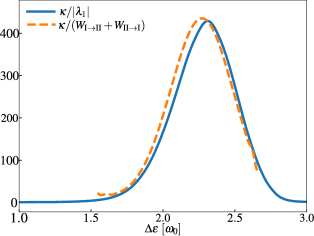
Figure 5: Comparison between the inverse of the smallest nonzero eigenvalue $|\lambda_{1}|$ of the Liouvillain (solid blue line) and $(W_{\mathrm{I}\rightarrow\mathrm{II}}+W_{\mathrm{II}\rightarrow\mathrm{I}})^{-1}$ as obtained by the two-state model (orange dashed line), as a function of the dot’s energy splitting $\Delta\varepsilon$. The curves are rescaled with the typical decay time of the oscillator $\kappa^{-1}$. Parameters: $Q=10^{3},\ \Gamma_{\mathrm{L}}=\Gamma_{\mathrm{R}}=0.1\omega_{0}$, $P=1$, $\lambda=0.13\omega_{0}$, $T=0$.

The two-state approximation for the system is valid if the $p_{n}$ distribution of the oscillator displays two distinct peaks of similar probability $\mathcal{P}_{\mathrm{I}}$ and $\mathcal{P}_{\mathrm{II}}$, which are well separated by a region with a negligible probability, as is reported in Fig. 1(e). To show telegraph noise, it is also necessary that the current variance associated to each state is smaller than the distance between the average values, i.e., $\Delta I_{\mathrm{I}},\ \Delta I_{\mathrm{II}}<|I_{\mathrm{I}}-I_{\mathrm{II}}|$, and that the switching rates between the two states are slow, such that one can resolve the individual jumps by monitoring the current during time. Under these conditions, we can model the current and the current noise by using a set of four parameters, $I_{\mathrm{I}}$, $I_{\mathrm{II}}$ and the rates $W_{\mathrm{I}\rightarrow\mathrm{II}}$ and $W_{\mathrm{II}\rightarrow\mathrm{I}}$. The two states will have relative probabilities

$$\mathcal{P}_{\mathrm{I}}=\frac{W_{\mathrm{II}\rightarrow\mathrm{I}}}{W_{\mathrm{I}\rightarrow\mathrm{II}}+W_{\mathrm{II}\rightarrow\mathrm{I}}},\quad\mathcal{P}_{\mathrm{II}}=\frac{W_{\mathrm{I}\rightarrow\mathrm{II}}}{W_{\mathrm{I}\rightarrow\mathrm{II}}+W_{\mathrm{II}\rightarrow\mathrm{I}}}.$$ (53)

The average current and the zero-frequency current noise are given by

$$I_{ts}=\frac{W_{\mathrm{II}\rightarrow\mathrm{I}}I_{\mathrm{I}}+W_{\mathrm{I}\rightarrow\mathrm{II}}I_{\mathrm{II}}}{W_{\mathrm{I}\rightarrow\mathrm{II}}+W_{\mathrm{II}\rightarrow\mathrm{I}}}$$ (54)

and

$$S(0)_{ts}=\frac{4\mathcal{P}_{\mathrm{I}}\mathcal{P}_{\mathrm{II}}(I_{\mathrm{I}}-I_{\mathrm{II}})^{2}}{W_{\mathrm{I}\rightarrow\mathrm{II}}+W_{\mathrm{II}\rightarrow\mathrm{I}}},$$ (55)

where the numerator is the two-state current variance [Harvey et al., 2008]. To calculate these quantities in our system, we identify $\mathcal{P}_{\mathrm{I}}$ and $\mathcal{P}_{\mathrm{II}}$ with the area of each of the two peaks in the steady-state $p_{n}$ distribution of the oscillator; next we set the elements of the density matrix corresponding to one of the two states to zero, and we build a new truncated density matrix from which one can calculate the two currents $I_{\mathrm{I}}$ and $I_{\mathrm{II}}$ through Eq. (51), hence the average current with Eq. (54). The current variance for each state can be estimated as $\Delta I_{\mathrm{I,II}}=\sqrt{\Gamma S_{\mathrm{I,II}}}$, where $S_{\mathrm{I,II}}$ is the zero-frequency noise calculated from Eq. (D), but using the truncated states. The sum of the rates $W_{\mathrm{I}\rightarrow\mathrm{II}}+W_{\mathrm{II}\rightarrow\mathrm{I}}$ is obtained by comparing the current noise calculated with Eq. (D) with the one given by Eq. (55). In the two-state model, a very slow timescale dominates the current noise. Specifically, this slow timescale is associated with the real part of the smallest nonzero eigenvalue of the Liouvillian of the system, as one can see directly by expanding Eq. (D) in terms of the eigenvalues and eigenvectors of $\mathcal{L}$ [Harvey et al., 2008]. If the lowest nonzero eigenvalue, $\lambda_{1}$, is small and well separated from the others (i.e., $|\lambda_{1}|\ll|\lambda_{p}|$ for $p>1$), the current noise is dominated by this eigenvalue, and a comparison with Eq. (55) leads us to identify $-\lambda_{1}=W_{\mathrm{I}\rightarrow\mathrm{II}}+W_{\mathrm{II}\rightarrow\mathrm{I}}$. In Fig. 5 we compare the result for the sum of the rates obtained by the eigenvalue expansion with the two-state approximation, showing that the behavior is very similar. Moreover, this timescale is much larger compared to the relaxation time of the oscillator, and shows indeed that the telegraph dynamics can be observed by monitoring the current. We stress that here we show relatively large coupling constants in order to realize numerical calculations with Fock occupation number not too large. On the other hand, semiclassical equations at finite polarization predict a similar behavior also at smaller coupling constants.

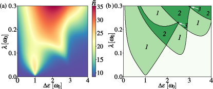
Figure 6: Effect of finite temperature and finite polarization. (a) Average occupation number in the oscillator at resonance as a function of the dot’s energy splitting $\Delta\varepsilon$ and of the spin-oscillator coupling strength $\lambda$. (b) Stability diagram of the oscillator. The italic numbers indicate the number of distinct peaks in the Fock distribution. Parameters: $Q=10^{3},\ \Gamma_{\mathrm{L}}=\Gamma_{\mathrm{R}}=0.1\omega_{0}$, $P=0.5$, $T=10\omega_{0}$.

Appendix F Multistability in nonideal cases

F.1 Effect of finite temperature $(T>0)$ and finite polarization $(P<1)$

The model system we considered can be implemented in a nanomechanical framework, by considering for example a carbon nanotube quantum dot (CNTQD). Mechanical resonators have in general low frequency ($\omega_{0}/2\pi\approx$100\text{\,}\mathrm{M}\mathrm{H}\mathrm{z}$$), and consequently one cannot neglect the effect of finite temperature of the thermal bath coupled to them, since $T\gtrsim\omega_{0}$. Furthermore, state-of-the-art ferromagnetic contacts reach a polarization of about 40-50%, thereby decreasing the lasing efficiency. In Fig. 6 we report the numerical calculation of the average occupation of the oscillator in the steady-state—obtained with Eq. (24)—together with the stability diagram for a nonideal case ($T\gg\omega_{0}$ and $P<1$), and we show how the qualitative picture is not destroyed. More specifically, the lasing threshold is pushed to a larger coupling, according to Eq. (26), as well as the onset of bi- and multistability. The thermal noise smears out the transitions to the lasing state.

F.2 Effect of spin relaxation at $T>0$ and $P<1$

We take into account decoherence in the quantum dot due to spin relaxation with a characteristic time $T_{1}$. We neglect a general inhomogeneous pure dephasing term of characteristic timescale $T_{\phi}$, which is justified as this term arises from hyperfine coupling of the electronic spin to the nuclear spin of ${}^{13}\mathrm{C}$ atoms, whose natural abundance in carbon is less than 1% [Churchill et al., 2009]. The spin relaxation is included in the dynamics by adding the dissipator $\mathcal{L}_{\mathrm{sr}}\hat{\rho}=\gamma_{\mathrm{sr}}\mathcal{D}(\hat{\sigma}_{-})\hat{\rho}$ to Eq. (24). $\gamma_{\mathrm{sr}}=T_{1}^{-1}$ identifies the relaxation rate. Spin relaxation plays a role similar to the effect of finite polarization: an electron decays into the lower spin level and then tunnels into the right lead, without emitting a quantum of oscillation. If the relaxation rate is much smaller than the Rabi frequency $\lambda A$ and of the tunneling rates, the dynamics is expected to be unperturbed. We find numerically the steady-state for the new Lindblad equation, and we calculate the average Fock number of the oscillator for different values of $\gamma_{\mathrm{sr}}$. An example is shown in Fig. 7(a) in which the lasing mechanism is noticeably suppressed only for $\gamma_{\mathrm{sr}}/\omega_{0}=${10}^{-2}$$. Figures 7(b) and 7(c) show the average occupation and the stability diagram as a function of $\lambda$ and $\Delta\varepsilon$. For the case of a CNTQD setup, the relaxation time in single-walled CNTs [Rice et al., 2013] was reported to be $T_{1}\approx$100\text{\,}\mathrm{\SIUnitSymbolMicro s}$$ at $T=$4\text{\,}\mathrm{K}$$ corresponding to a relaxation rate of $10\,\,\mbox{kHz}$. At low temperature ($T\approx 20\,\,\mbox{mK}$, considered in our case) we expect a substantial decrease of this value.

F.3 Effect of nonlinearity at $T>0$ and $P<1$

We include in our numerical model a Duffing nonlinearity for the harmonic oscillator, by modifying Hamiltonian (1) into

$$\hat{H}=\frac{\Delta\varepsilon}{2}\hat{\sigma}_{z}+\omega_{0}\hat{b}^{\dagger}\hat{b}+\frac{\tilde{\beta}}{4}(\hat{b}+\hat{b}^{\dagger})^{4}+\lambda(\hat{\sigma}_{+}+\hat{\sigma}_{-})(\hat{b}+\hat{b}^{\dagger}).$$ (56)

We introduced the parameter $\tilde{\beta}=\beta x^{4}_{\mathrm{ZPM}}$, with $\beta$ and $x_{\mathrm{ZPM}}=\sqrt{\hbar/2m\omega_{0}}$ being the Duffing nonlinearity parameter and the zero-point amplitude of the oscillator (where we have restored $\hbar$), respectively. The nonlinearity is expected to play a nonneglibile role for mechanical resonators where intrinsic nonlinearities can be large and hence might affect the lasing behavior at large amplitudes. For a realistic estimate of $\tilde{\beta}$, we set the typical mass of a CNT to be $m\approx${10}^{-21}$$ kg, which for $\omega_{0}/2\pi=$100\text{\,}\mathrm{M}\mathrm{H}\mathrm{z}$$ gives zero-point fluctuations of order $x_{\mathrm{ZPM}}\approx$10\text{\,}\mathrm{pm}$$. Experimentally, the geometrical nonlinearity parameter for a CNT is positive and of order $\beta/m=${10}^{35}\text{\,}\mathrm{N}\text{\,}{\mathrm{kg}}^{-1}\text{\,}{\mathrm{m}}^{-3}$$ [Meerwaldt et al., 2012]. The parameter $\tilde{\beta}/2\pi$ is hence of order $\approx$1\text{\,}\mathrm{k}\mathrm{H}\mathrm{z}$$, i.e., $\tilde{\beta}/\omega_{0}\approx${10}^{-5}$$. We neglect the electrostatic nonlinearity arising from strong coupling effects between the leads and the CNT and from single-electron tunneling, which is in general orders of magnitude smaller and is proportional to the electron tunneling rate, assumed much smaller than $\omega_{0}$. Solving the Lindblad equation for the steady-state, we report the average Fock number as a function of the coupling strength $\lambda$ in Fig. 8(a). Finally, in Fig. 8(b,c) we show the average occupation and the stability diagram as a function of $\lambda$ and $\Delta\varepsilon$ by combining the effect of finite temperature, finite polarization, spin relaxation and Duffing nonlinearity showing that the main features still persist in a largely nonideal case.

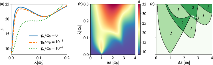
Figure 7: Effect of dot’s spin relaxation. (a) Average occupation of the oscillator on resonance as a function of $\lambda$ at different values of the spin relaxation rate $\gamma_{\mathrm{sr}}$. (b) Average occupation of the oscillator as a function of $\lambda$ and of $\Delta\varepsilon$ for $\gamma_{\mathrm{sr}}=10^{-3}\omega_{0}$. (c) Stability diagram of the oscillator for $\gamma_{\mathrm{sr}}=10^{-3}\omega_{0}$: the italic numbers indicate the number of distinct peaks in the Fock distribution. Parameters: $Q=10^{3}$, $\Gamma_{\mathrm{L}}=\Gamma_{\mathrm{R}}=0.1\omega_{0}$, $P=0.5$, $T=10\omega_{0}$.

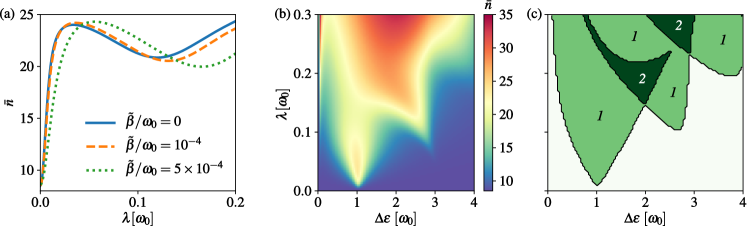
Figure 8: Effect of the Duffing nonlinearity for a nanomechanical resonator. (a) Average occupation for the oscillator as a function of $\lambda$ for three different values of the Duffing nonlinearity parameter and $\gamma_{\mathrm{sr}}=0$. (b) Average occupation for the oscillator as a function $\lambda$ and $\Delta\varepsilon$ for $\gamma_{\mathrm{sr}}=10^{-3}\omega_{0}$ and $\tilde{\beta}=10^{-4}\omega_{0}$. (c) Stability diagram of the oscillator for $\gamma_{\mathrm{sr}}=10^{-3}\omega_{0}$ and $\tilde{\beta}=10^{-4}\omega_{0}$: the italic numbers indicate the number of distinct peaks in the Fock distribution. Parameters: $Q=10^{3}$, $\Gamma_{\mathrm{L}}=\Gamma_{\mathrm{R}}=0.1\omega_{0}$, $P=0.5$, $T=10\omega_{0}$.

References

- Liu et al. (2015) Y.-Y. Liu, J. Stehlik, C. Eichler, M. J. Gullans, J. M. Taylor, and J. R. Petta, Semiconductor double quantum dot micromaser, Science 347, 285 (2015).
- Mi et al. (2016) X. Mi, J. V. Cady, D. M. Zajac, P. W. Deelman, and J. R. Petta, Strong coupling of a single electron in silicon to a microwave photon, Science 355, 156 (2016).
- Viennot et al. (2015) J. J. Viennot, M. C. Dartiailh, A. Cottet, and T. Kontos, Coherent coupling of a single spin to microwave cavity photons, Science 349, 408 (2015).
- Stockklauser et al. (2015) A. Stockklauser, V. F. Maisi, J. Basset, K. Cujia, C. Reichl, W. Wegscheider, T. Ihn, A. Wallraff, and K. Ensslin, Microwave Emission from Hybridized States in a Semiconductor Charge Qubit, Phys. Rev. Lett. 115, 046802 (2015).
- Stockklauser et al. (2017) A. Stockklauser, P. Scarlino, J. V. Koski, S. Gasparinetti, C. K. Andersen, C. Reichl, W. Wegscheider, T. Ihn, K. Ensslin, and A. Wallraff, Strong Coupling Cavity QED with Gate-Defined Double Quantum Dots Enabled by a High Impedance Resonator, Phys. Rev. X 7, 011030 (2017).
- Li et al. (2018) Y. Li, S.-X. Li, F. Gao, H.-O. Li, G. Xu, K. Wang, D. Liu, G. Cao, M. Xiao, T. Wang, J.-J. Zhang, G.-C. Guo, and G.-P. Guo, Coupling a Germanium Hut Wire Hole Quantum Dot to a Superconducting Microwave Resonator, Nano Lett. 18, 2091 (2018).
- Naik et al. (2006) A. Naik, O. Buu, M. D. LaHaye, A. D. Armour, A. A. Clerk, M. P. Blencowe, and K. C. Schwab, Cooling a nanomechanical resonator with quantum back-action, Nature 443, 193 (2006).
- Benyamini et al. (2014) A. Benyamini, A. Hamo, S. V. Kusminskiy, F. von Oppen, and S. Ilani, Real-space tailoring of the electron–phonon coupling in ultraclean nanotube mechanical resonators, Nat. Phys. 10, 151 (2014).
- Okazaki et al. (2016) Y. Okazaki, I. Mahboob, K. Onomitsu, S. Sasaki, and H. Yamaguchi, Gate-controlled electromechanical backaction induced by a quantum dot, Nat. Comm. 7, 11132 (2016).
- Deng et al. (2016) G.-W. Deng, D. Zhu, X.-H. Wang, C.-L. Zou, J.-T. Wang, H.-O. Li, G. Cao, D. Liu, Y. Li, M. Xiao, G.-C. Guo, K.-L. Jiang, X.-C. Dai, and G.-P. Guo, Strongly Coupled Nanotube Electromechanical Resonators, Nano Lett. 16, 5456 (2016).
- Lambert et al. (2015) N. Lambert, F. Nori, and C. Flindt, Bistable Photon Emission from a Solid-State Single-Atom Laser, Phys. Rev. Lett. 115, 216803 (2015).
- Parafilo et al. (2016) A. V. Parafilo, S. I. Kulinich, L. Y. Gorelik, M. N. Kiselev, R. I. Shekhter, and M. Jonson, Spin-mediated Photomechanical Coupling of a Nanoelectromechanical Shuttle, Phys. Rev. Lett. 117, 057202 (2016).
- Filipowicz et al. (1986) P. Filipowicz, J. Javanainen, and P. Meystre, Theory of a microscopic maser, Phys. Rev. A 34, 3077 (1986).
- Lugiato et al. (1987) L. A. Lugiato, M. O. Scully, and H. Walther, Connection between microscopic and macroscopic maser theory, Phys. Rev. A 36, 740 (1987).
- Mu and Savage (1992) Y. Mu and C. M. Savage, One-atom lasers, Phys. Rev. A 46, 5944 (1992).
- Rice and Carmichael (1994) P. R. Rice and H. J. Carmichael, Photon statistics of a cavity-QED laser: A comment on the laser–phase-transition analogy, Phys. Rev. A 50, 4318 (1994).
- Wang and Vyas (1996) C. Wang and R. Vyas, Fokker-Planck equation in the good-cavity limit and single-atom optical bistability, Phys. Rev. A 54, 4453 (1996).
- Walther et al. (2006) H. Walther, B. T. H. Varcoe, B.-G. Englert, and T. Becker, Cavity quantum electrodynamics, Rep. Prog. Phys. 69, 1325 (2006).
- Doiron et al. (2006) C. B. Doiron, W. Belzig, and C. Bruder, Electrical transport through a single-electron transistor strongly coupled to an oscillator, Phys. Rev. B 74, 205336 (2006).
- Rodrigues et al. (2007a) D. A. Rodrigues, J. Imbers, and A. D. Armour, Quantum Dynamics of a Resonator Driven by a Superconducting Single-Electron Transistor: A Solid-State Analogue of the Micromaser, Phys. Rev. Lett. 98, 067204 (2007a).
- Rodrigues et al. (2007b) D. A. Rodrigues, J. Imbers, T. J. Harvey, and A. D. Armour, Dynamical instabilities of a resonator driven by a superconducting single-electron transistor, New J. Phys. 9, 84 (2007b).
- Micchi et al. (2015) G. Micchi, R. Avriller, and F. Pistolesi, Mechanical Signatures of the Current Blockade Instability in Suspended Carbon Nanotubes, Phys. Rev. Lett. 115, 206802 (2015).
- Marquardt et al. (2006) F. Marquardt, J. G. E. Harris, and S. M. Girvin, Dynamical Multistability Induced by Radiation Pressure in High-Finesse Micromechanical Optical Cavities, Phys. Rev. Lett. 96, 103901 (2006).
- Nation (2013) P. D. Nation, Nonclassical mechanical states in an optomechanical micromaser analog, Phys. Rev. A 88, 053828 (2013).
- McKeever et al. (2003) J. McKeever, A. Boca, A. D. Boozer, J. R. Buck, and H. J. Kimble, Experimental realization of a one-atom laser in the regime of strong coupling, Nature 425, 268 (2003).
- Astafiev et al. (2007) O. Astafiev, K. Inomata, A. O. Niskanen, T. Yamamoto, Y. A. Pashkin, Y. Nakamura, and J. S. Tsai, Single artificial-atom lasing, Nature 449, 588 (2007).
- Liu et al. (2017) Y.-Y. Liu, J. Stehlik, C. Eichler, X. Mi, T. R. Hartke, M. J. Gullans, J. M. Taylor, and J. R. Petta, Threshold Dynamics of a Semiconductor Single Atom Maser, Phys. Rev. Lett. 119, 097702 (2017).
- Childress et al. (2004) L. Childress, A. S. Sørensen, and M. D. Lukin, Mesoscopic cavity quantum electrodynamics with quantum dots, Phys. Rev. A 69, 042302 (2004).
- Jin et al. (2011) P.-Q. Jin, M. Marthaler, J. H. Cole, A. Shnirman, and G. Schön, Lasing and transport in a quantum-dot resonator circuit, Phys. Rev. B 84, 035322 (2011).
- Liu et al. (2014) Y.-Y. Liu, K. D. Petersson, J. Stehlik, J. M. Taylor, and J. R. Petta, Photon Emission from a Cavity-Coupled Double Quantum Dot, Phys. Rev. Lett. 113, 036801 (2014).
- Brandes and Lambert (2003) T. Brandes and N. Lambert, Steering of a bosonic mode with a double quantum dot, Phys. Rev. B 67, 125323 (2003).
- Bergenfeldt and Samuelsson (2013) C. Bergenfeldt and P. Samuelsson, Nonlocal transport properties of nanoscale conductor–microwave cavity systems, Phys. Rev. B 87, 195427 (2013).
- Gullans et al. (2015) M. J. Gullans, Y.-Y. Liu, J. Stehlik, J. R. Petta, and J. M. Taylor, Phonon-Assisted Gain in a Semiconductor Double Quantum Dot Maser, Phys. Rev. Lett. 114, 196802 (2015).
- Khaetskii et al. (2013) A. Khaetskii, V. N. Golovach, X. Hu, and I. Žutić, Proposal for a Phonon Laser Utilizing Quantum-Dot Spin States, Phys. Rev. Lett. 111, 186601 (2013).
- Scully and Zubairy (1997) M. Scully and M. Zubairy, Quantum Optics (Cambridge University Press, Cambridge, 1997).
- (36) P. Forn-Díaz, L. Lamata, E. Rico, J. Kono, and E. Solano, Ultrastrong coupling regimes of light-matter interaction, arXiv:1804.09275 .
- Kockum et al. (2019) A. F. Kockum, A. Miranowicz, S. De Liberato, S. Savasta, and F. Nori, Ultrastrong coupling between light and matter, Nat. Rev. Phys. 1, 19 (2019).
- Breuer and Petruccione (2002) H.-P. Breuer and F. Petruccione, The Theory of Open Quantum Systems (Oxford University Press, Oxford, 2002).
- Timm (2008) C. Timm, Tunneling through molecules and quantum dots: Master-equation approaches, Phys. Rev. B 77, 195416 (2008).
- Cohen-Tannoudji et al. (1992) C. Cohen-Tannoudji, J. Dupont-Roc, and G. Grynberg, Atom-Photon Interactions (Wiley, New York, 1992).
- Johansson et al. (2012) J. Johansson, P. Nation, and F. Nori, QuTiP: An open-source Python framework for the dynamics of open quantum systems, Comput. Phys. Commun. 183, 1760 (2012).
- Johansson et al. (2013) J. Johansson, P. Nation, and F. Nori, QuTiP 2: A Python framework for the dynamics of open quantum systems, Comput. Phys. Commun. 184, 1234 (2013).
- Kirton and Armour (2013) P. G. Kirton and A. D. Armour, Nonlinear dynamics of a driven nanomechanical single-electron transistor, Phys. Rev. B 87, 155407 (2013).
- Flindt et al. (2004) C. Flindt, T. Novotný, and A.-P. Jauho, Current noise in a vibrating quantum dot array, Phys. Rev. B 70, 205334 (2004).
- Flindt et al. (2005) C. Flindt, T. Novotný, and A.-P. Jauho, Full counting statistics of nano-electromechanical systems, EPL (Europhysics Letters) 69, 475 (2005).
- Flindt et al. (2010) C. Flindt, T. Novotný, A. Braggio, and A.-P. Jauho, Counting statistics of transport through Coulomb blockade nanostructures: High-order cumulants and non-Markovian effects, Phys. Rev. B 82, 155407 (2010).
- Usmani et al. (2007) O. Usmani, Y. M. Blanter, and Y. V. Nazarov, Strong feedback and current noise in nanoelectromechanical systems, Phys. Rev. B 75, 195312 (2007).
- Brüggemann et al. (2012) J. Brüggemann, G. Weick, F. Pistolesi, and F. von Oppen, Large current noise in nanoelectromechanical systems close to continuous mechanical instabilities, Phys. Rev. B 85, 125441 (2012).
- Harvey et al. (2008) T. J. Harvey, D. A. Rodrigues, and A. D. Armour, Current noise of a superconducting single-electron transistor coupled to a resonator, Phys. Rev. B 78, 024513 (2008).
- Meerwaldt et al. (2012) H. Meerwaldt, G. Steele, and H. S. J. van der Zant, Carbon nanotubes: Nonlinear high-Q resonators with strong coupling to single-electron tunneling, in Fluctuating Nonlinear Oscillators: From Nanomechanics to Quantum Superconducting Circuits, edited by M. I. Dykman (Oxford University Press, Oxford, 2012).
- Sahoo et al. (2005) S. Sahoo, T. Kontos, J. Furer, C. Hoffmann, M. Gräber, A. Cottet, and C. Schönenberger, Electric field control of spin transport, Nat. Phys. 1, 99 (2005).
- Rice et al. (2013) W. D. Rice, R. T. Weber, P. Nikolaev, S. Arepalli, V. Berka, A. L. Tsai, and J. Kono, Spin relaxation times of single-wall carbon nanotubes, Phys. Rev. B 88, 041401 (2013).
- Churchill et al. (2009) H. O. H. Churchill, F. Kuemmeth, J. W. Harlow, A. J. Bestwick, E. I. Rashba, K. Flensberg, C. H. Stwertka, T. Taychatanapat, S. K. Watson, and C. M. Marcus, Relaxation and Dephasing in a Two-Electron Nanotube Double Quantum Dot, Phys. Rev. Lett. 102, 166802 (2009).
- Moser et al. (2014) J. Moser, A. Eichler, J. Güttinger, M. I. Dykman, and A. Bachtold, Nanotube mechanical resonators with quality factors of up to 5 million, Nat. Nanotechnol. 9, 1007 (2014).
- Pályi et al. (2012) A. Pályi, P. R. Struck, M. Rudner, K. Flensberg, and G. Burkard, Spin-Orbit-Induced Strong Coupling of a Single Spin to a Nanomechanical Resonator, Phys. Rev. Lett. 108, 206811 (2012).
- Stadler et al. (2014) P. Stadler, W. Belzig, and G. Rastelli, Ground-State Cooling of a Carbon Nanomechanical Resonator by Spin-Polarized Current, Phys. Rev. Lett. 113, 047201 (2014).
- Stadler et al. (2015) P. Stadler, W. Belzig, and G. Rastelli, Control of vibrational states by spin-polarized transport in a carbon nanotube resonator, Phys. Rev. B 91, 085432 (2015).
- Ranjan et al. (2015) V. Ranjan, G. Puebla-Hellmann, M. Jung, T. Hasler, A. Nunnenkamp, M. Muoth, C. Hierold, A. Wallraff, and C. Schönenberger, Clean carbon nanotubes coupled to superconducting impedance-matching circuits, Nat. Comm. 6, 7165 (2015).
- Mi et al. (2018) X. Mi, M. Benito, S. Putz, D. M. Zajac, J. M. Taylor, G. Burkard, and J. R. Petta, A coherent spin–photon interface in silicon, Nature 555, 599 (2018).