CoLa: Decentralized Linear Learning

Abstract

Decentralized machine learning is a promising emerging paradigm in view of global challenges of data ownership and privacy. We consider learning of linear classification and regression models, in the setting where the training data is decentralized over many user devices, and the learning algorithm must run on-device, on an arbitrary communication network, without a central coordinator. We propose CoLa, a new decentralized training algorithm with strong theoretical guarantees and superior practical performance. Our framework overcomes many limitations of existing methods, and achieves communication efficiency, scalability, elasticity as well as resilience to changes in data and allows for unreliable and heterogeneous participating devices.

1 Introduction

With the immense growth of data, decentralized machine learning has become not only attractive but a necessity. Personal data from, for example, smart phones, wearables and many other mobile devices is sensitive and exposed to a great risk of data breaches and abuse when collected by a centralized authority or enterprise. Nevertheless, many users have gotten accustomed to giving up control over their data in return for useful machine learning predictions (e.g. recommendations), which benefits from joint training on the data of all users combined in a centralized fashion.

In contrast, decentralized learning aims at learning this same global machine learning model, without any central server. Instead, we only rely on distributed computations of the devices themselves, with each user’s data never leaving its device of origin. While increasing research progress has been made towards this goal, major challenges in terms of the privacy aspects as well as algorithmic efficiency, robustness and scalability remain to be addressed. Motivated by aforementioned challenges, we make progress in this work addressing the important problem of training generalized linear models in a fully decentralized environment.

Existing research on decentralized optimization, $\min_{{\bf x}\in{\mathbb{R}}^{n}}F({\bf x})$, can be categorized into two main directions. The seminal line of work started by Bertsekas and Tsitsiklis in the 1980s, cf. (Tsitsiklis et al., 1986), tackles this problem by splitting the parameter vector ${\bf x}$ by coordinates/components among the devices. A second more recent line of work including e.g. (Nedic and Ozdaglar, 2009; Duchi et al., 2012; Shi et al., 2015; Mokhtari and Ribeiro, 2016; Nedic et al., 2017) addresses sum-structured $F({\bf x})=\sum_{k}F_{k}({\bf x})$ where $F_{k}$ is the local cost function of node $k$. This structure is closely related to empirical risk minimization in a learning setting. See e.g. (Cevher et al., 2014) for an overview of both directions. While the first line of work typically only provides convergence guarantees for smooth objectives $F$, the second approach often suffers from a “lack of consensus”, that is, the minimizers of $\{F_{k}\}_{k}$ are typically different since the data is not distributed i.i.d. between devices in general.

Contributions.

In this paper, our main contribution is to propose CoLa, a new decentralized framework for training generalized linear models with convergence guarantees. Our scheme resolves both described issues in existing approaches, using techniques from primal-dual optimization, and can be seen as a generalization of CoCoA (Smith et al., 2018) to the decentralized setting. More specifically, the proposed algorithm offers

• Convergence Guarantees: Linear and sublinear convergence rates are guaranteed for strongly convex and general convex objectives respectively. Our results are free of the restrictive assumptions made by stochastic methods (Zhang et al., 2015; Wang et al., 2017), which requires i.i.d. data distribution over all devices.

• Communication Efficiency and Usability: Employing a data-local subproblem between each communication round, CoLa not only achieves communication efficiency but also allows the re-use of existing efficient single-machine solvers for on-device learning. We provide practical decentralized primal-dual certificates to diagnose the learning progress.

• Elasticity and Fault Tolerance: Unlike sum-structured approaches such as SGD, CoLa is provably resilient to changes in the data, in the network topology, and participating devices disappearing, straggling or re-appearing in the network.

Our implementation is publicly available under github.com/epfml/cola .

1.1 Problem statement

Setup. Many machine learning and signal processing models are formulated as a composite convex optimization problem of the form

$$\min_{\mathbf{u}}\;l(\mathbf{u})+r(\mathbf{u}),$$

where $l$ is a convex loss function of a linear predictor over data and $r$ is a convex regularizer. Some cornerstone applications include e.g. logistic regression, SVMs, Lasso, generalized linear models, each combined with or without L1, L2 or elastic-net regularization. Following the setup of (Dünner et al., 2016; Smith et al., 2018), these training problems can be mapped to either of the two following formulations, which are dual to each other

$$\min_{{\bf x}\in{\mathbb{R}}^{n}}\big{[}F_{A}({\bf x}):=f(\mathbf{A}{\bf x})+\textstyle\sum_{i}g_{i}(x_{i})\ \big{]}$$ (A)

$$\min_{{\bf w}\in{\mathbb{R}}^{d}}\big{[}F_{B}(\mathbf{w}):=f^{*}(\mathbf{w})+\textstyle\sum_{i}g_{i}^{*}(-\mathbf{A}_{i}^{\top}\mathbf{w})\big{]},$$ (B)

where $f^{*},g^{*}_{i}$ are the convex conjugates of $f$ and $g_{i}$, respectively. Here ${\bf x}\in{\mathbb{R}}^{n}$ is a parameter vector and $\mathbf{A}:=[\mathbf{A}_{1};\ldots;\mathbf{A}_{n}]\in{\mathbb{R}}^{d\times n}$ is a data matrix with column vectors $\mathbf{A}_{i}\in{\mathbb{R}}^{d},i\in[n]$. We assume that $f$ is smooth (Lipschitz gradient) and $g({\bf x}):=\sum_{i=1}^{n}g_{i}(x_{i})$ is separable.

Data partitioning. As in (Jaggi et al., 2014; Dünner et al., 2016; Smith et al., 2018), we assume the dataset $\mathbf{A}$ is distributed over $K$ machines according to a partition $\{\mathcal{P}_{k}\}_{k=1}^{K}$ of the columns of $\mathbf{A}$. Note that this convention maintains the flexibility of partitioning the training dataset either by samples (through mapping applications to (B), e.g. for SVMs) or by features (through mapping applications to (A), e.g. for Lasso or L1-regularized logistic regression). For ${\bf x}\in{\mathbb{R}}^{n}$, we write ${\bf x}_{[k]}\in{\mathbb{R}}^{n}$ for the $n$-vector with elements $({\bf x}_{[k]})_{i}:=x_{i}$ if $i\in\mathcal{P}_{k}$ and $({\bf x}_{[k]})_{i}:=0$ otherwise, and analogously $\mathbf{A}_{[k]}\in{\mathbb{R}}^{d\times n_{k}}$ for the corresponding set of local data columns on node $k$, which is of size $n_{k}=|\mathcal{P}_{k}|$.

Network topology. We consider the task of joint training of a global machine learning model in a decentralized network of $K$ nodes. Its connectivity is modelled by a mixing matrix $\mathcal{W}\in{\mathbb{R}}_{+}^{K\times K}$. More precisely, $\mathcal{W}_{ij}\in[0,1]$ denotes the connection strength between nodes $i$ and $j$, with a non-zero weight indicating the existence of a pairwise communication link. We assume $\mathcal{W}$ to be symmetric and doubly stochastic, which means each row and column of $\mathcal{W}$ sums to one.

The spectral properties of $\mathcal{W}$ used in this paper are that the eigenvalues of $\mathcal{W}$ are real, and $1=\lambda_{1}(\mathcal{W})\geq\cdots\geq\lambda_{n}(\mathcal{W})\geq-1$. Let the second largest magnitude of the eigenvalues of $\mathcal{W}$ be $\beta:=\max\{|\lambda_{2}(\mathcal{W})|,|\lambda_{n}(\mathcal{W})|\}$. $1-\beta$ is called the spectral gap, a quantity well-studied in graph theory and network analysis. The spectral gap measures the level of connectivity among nodes. In the extreme case when $\mathcal{W}$ is diagonal, and thus an identity matrix, the spectral gap is 0 and there is no communication among nodes. To ensure convergence of decentralized algorithms, we impose the standard assumption of positive spectral gap of the network which includes all connected graphs, such as e.g. a ring or 2-D grid topology, see also Appendix B for details.

1.2 Related work

Research in decentralized optimization dates back to the 1980s with the seminal work of Bertsekas and Tsitsiklis, cf. (Tsitsiklis et al., 1986). Their framework focuses on the minimization of a (smooth) function by distributing the components of the parameter vector ${\bf x}$ among agents. In contrast, a second more recent line of work (Nedic and Ozdaglar, 2009; Duchi et al., 2012; Shi et al., 2015; Mokhtari and Ribeiro, 2016; Nedic et al., 2017; Scaman et al., 2017, 2018) considers minimization of a sum of individual local cost-functions $F({\bf x})=\sum_{i}F_{i}({\bf x})$, which are potentially non-smooth. Our work here can be seen as bridging the two scenarios to the primal-dual setting (A) and (B).

While decentralized optimization is a relatively mature area in the operations research and automatic control communities, it has recently received a surge of attention for machine learning applications, see e.g. (Cevher et al., 2014). Decentralized gradient descent (DGD) with diminishing stepsizes was proposed by (Nedic and Ozdaglar, 2009; Jakovetic et al., 2012), showing convergence to the optimal solution at a sublinear rate. (Yuan et al., 2016) further prove that DGD will converge to the neighborhood of a global optimum at a linear rate when used with a constant stepsize for strongly convex objectives. (Shi et al., 2015) present EXTRA, which offers a significant performance boost compared to DGD by using a gradient tracking technique. (Nedic et al., 2017) propose the DIGing algorithm to handle a time-varying network topology. For a static and symmetric $\mathcal{W}$, DIGing recovers EXTRA by redefining the two mixing matrices in EXTRA. The dual averaging method (Duchi et al., 2012) converges at a sublinear rate with a dynamic stepsize. Under a strong convexity assumption, decomposition techniques such as decentralized ADMM (DADMM, also known as consensus ADMM) have linear convergence for time-invariant undirected graphs, if subproblems are solved exactly (Shi et al., 2014; Wei and Ozdaglar, 2013). DADMM+ (Bianchi et al., 2016) is a different primal-dual approach with more efficient closed-form updates in each step (as compared to ADMM), and is proven to converge but without a rate. Compared to CoLa, neither of DADMM and DADMM+ can be flexibly adapted to the communication-computation tradeoff due to their fixed update definition, and both require additional hyperparameters to tune in each use-case (including the $\rho$ from ADMM). Notably CoLa shows superior performance compared to DIGing and decentralized ADMM in our experiments. (Scaman et al., 2017, 2018) present lower complexity bounds and optimal algorithms for objectives in the form $F({\bf x})=\sum_{i}F_{i}({\bf x})$. Specifically, (Scaman et al., 2017) assumes each $F_{i}({\bf x})$ is smooth and strongly convex, and (Scaman et al., 2018) assumes each $F_{i}({\bf x})$ is Lipschitz continuous and convex. Additionally (Scaman et al., 2018) needs a boundedness constraint for the input problem. In contrast, CoLa can handle non-smooth and non-strongly convex objectives (A) and (B), suited to the mentioned applications in machine learning and signal processing. For smooth nonconvex models, (Lian et al., 2017) demonstrate that a variant of decentralized parallel SGD can outperform the centralized variant when the network latency is high. They further extend it to the asynchronous setting (Lian et al., 2018) and to deal with large data variance among nodes (Tang et al., 2018a) or with unreliable network links (Tang et al., 2018b). For the decentralized, asynchronous consensus optimization, (Wu et al., 2018) extends the existing PG-EXTRA and proves convergence of the algorithm. (Sirb and Ye, 2018) proves a $O(K/\epsilon^{2})$ rate for stale and stochastic gradients. (Lian et al., 2018) achieves $O(1/\epsilon)$ rate and has linear speedup with respect to number of workers.

In the distributed setting with a central server, algorithms of the CoCoA family (Yang, 2013; Jaggi et al., 2014; Ma et al., 2015; Dünner et al., 2018)—see (Smith et al., 2018) for a recent overview—are targeted for problems of the forms (A) and (B). For convex models, CoCoA has shown to significantly outperform competing methods including e.g., ADMM, distributed SGD etc. Other centralized algorithm representatives are parallel SGD variants such as (Agarwal and Duchi, 2011; Zinkevich et al., 2010) and more recent distributed second-order methods (Zhang and Lin, 2015; Reddi et al., 2016; Gargiani, 2017; Lee and Chang, 2017; Dünner et al., 2018; Lee et al., 2018).

In this paper we extend CoCoA to the challenging decentralized environment—with no central coordinator—while maintaining all of its nice properties. We are not aware of any existing primal-dual methods in the decentralized setting, except the recent work of (Smith et al., 2017) on federated learning for the special case of multi-task learning problems. Federated learning was first described by (Konecnỳ et al., 2015, 2016; McMahan et al., 2017) as decentralized learning for on-device learning applications, combining a global shared model with local personalized models. Current federated optimization algorithms (like FedAvg in (McMahan et al., 2017)) are still close to the centralized setting. In contrast, our work provides a fully decentralized alternative algorithm for federated learning with generalized linear models.

2 The decentralized algorithm: CoLa

The CoLa framework is summarized in Algorithm 1. For a given input problem we map it to either of the (A) or (B) formulation, and define the locally stored dataset $\mathbf{A}_{[k]}$ and local part of the weight vector $\mathbf{x}_{[k]}$ in node $k$ accordingly. While ${\bf v}=\mathbf{A}\mathbf{x}$ is the shared state being communicated in CoCoA, this is generally unknown to a node in the fully decentralized setting. Instead, we maintain ${\bf v}_{k}$, a local estimate of ${\bf v}$ in node $k$, and use it as a surrogate in the algorithm.

1 Input: Data matrix $\mathbf{A}$ distributed column-wise according to partition $\{\mathcal{P}_{k}\}_{k=1}^{K}$. Mixing matrix $\mathcal{W}$. Aggregation parameter $\gamma\!\in\![0,1]$, and local subproblem parameter $\sigma^{\prime}$ as in 1. Starting point ${\bf x}^{(0)}:={\bf 0}\in{\mathbb{R}}^{n}$, ${\bf v}^{(0)}:={\bf 0}\in{\mathbb{R}}^{d}$, ${\bf v}^{(0)}_{k}:={\bf 0}\in{\mathbb{R}}^{d}~{}\forall~{}k=1,\ldots K$;

2for $t=0,1,2,\dots,T$ do

3       for $k\in\{1,2,\dots,K\}$ in parallel over all nodes do

4            

5            compute locally averaged shared vector ${\bf v}^{(t+\frac{1}{2})}_{k}:=\textstyle\sum_{l=1}^{K}\mathcal{W}_{kl}{\bf v}^{(t)}_{l}$

6            

7            $\Delta{\bf x}_{[k]}\leftarrow$ $\Theta$-approximate solution to subproblem (1) at ${\bf v}^{(t+\frac{1}{2})}_{k}$

8            [-1mm] update local variable ${\bf x}^{(t+1)}_{[k]}:={\bf x}^{(t)}_{[k]}+\gamma\,\Delta{\bf x}_{[k]}$

9             compute update of local estimate $\Delta{\bf v}_{k}:=\mathbf{A}_{[k]}\Delta{\bf x}_{[k]}$

10            

11            ${\bf v}^{(t+1)}_{k}:={\bf v}^{(t+\frac{1}{2})}_{k}+\gamma K\Delta{\bf v}_{k}$

12       end for

13      

14 end for

Algorithm 1 CoLa: Communication-Efficient Decentralized Linear Learning

New data-local quadratic subproblems. During a computation step, node $k$ locally solves the following minimization problem

$$\min_{\Delta{\bf x}_{[k]}\in{\mathbb{R}}^{n}}\ \mathscr{G}^{\sigma^{\prime}}_{k}(\Delta{\bf x}_{[k]};\mathbf{v}_{k},{\bf x}_{[k]}),\vspace{-2mm}$$ (1)

where

$$\begin{split}\textstyle\mathscr{G}^{\sigma^{\prime}}_{k}(\Delta{\bf x}_{[k]};\mathbf{v}_{k},{\bf x}_{[k]}):=\ &\textstyle\frac{1}{K}f(\mathbf{v}_{k})+\nabla f(\mathbf{v}_{k})^{\top}\mathbf{A}_{[k]}\Delta{\bf x}_{[k]}\\ &\textstyle+\frac{\sigma^{\prime}}{2\tau}\left\lVert{\mathbf{A}_{[k]}\Delta{\bf x}_{[k]}}\right\rVert^{2}+\sum_{i\in\mathcal{P}_{k}}g_{i}(x_{i}+{(\Delta{\bf x}_{[k]})}_{i}).\end{split}$$ (2)

Crucially, this subproblem only depends on the local data $\mathbf{A}_{[k]}$, and local vectors ${\bf v}_{l}$ from the neighborhood of the current node $k$. In contrast, in CoCoA (Smith et al., 2018) the subproblem is defined in terms of a global aggregated shared vector ${\bf v}_{c}:=\mathbf{A}{\bf x}\in{\mathbb{R}}^{d}$, which is not available in the decentralized setting. The aggregation parameter $\gamma\in[0,1]$ does not need to be tuned; in fact, we use the default $\gamma:=1$ throughout the paper, see (Ma et al., 2015) for a discussion. Once $\gamma$ is settled, a safe choice of the subproblem relaxation parameter $\sigma^{\prime}$ is given as $\sigma^{\prime}:=\gamma K$. $\sigma^{\prime}$ can be additionally tightened using an improved Hessian subproblem (Section E.3).

Algorithm description. At time $t$ on node $k$, ${\bf v}^{(t+\frac{1}{2})}_{k}$ is a local estimate of the shared variable after a communication step (i.e. gossip mixing). The local subproblem (1) based on this estimate is solved and yields $\Delta{\bf x}_{[k]}$. Then we calculate $\Delta{\bf v}_{k}:=\mathbf{A}_{[k]}\Delta{\bf x}_{[k]}$, and update the local shared vector ${\bf v}^{(t+1)}_{k}$. We allow the local subproblem to be solved approximately:

Assumption 1 ($\Theta$-approximation solution).

Let $\Theta\in[0,1]$ be the relative accuracy of the local solver (potentially randomized), in the sense of returning an approximate solution $\Delta{\bf x}_{[k]}$ at each step $t$, s.t.

$$\frac{\mathbb{E}[\mathscr{G}^{\sigma^{\prime}}_{k}(\Delta{\bf x}_{[k]};\mathbf{v}_{k},{\bf x}_{[k]})-\mathscr{G}^{\sigma^{\prime}}_{k}(\Delta{\bf x}^{\star}_{[k]};\mathbf{v}_{k},{\bf x}_{[k]})]}{~{}~{}\mathscr{G}^{\sigma^{\prime}}_{k}(~{}~{}{\bf 0}~{}~{}~{}~{};\mathbf{v}_{k},{\bf x}_{[k]})~{}-\mathscr{G}^{\sigma^{\prime}}_{k}(\Delta{\bf x}^{\star}_{[k]};\mathbf{v}_{k},{\bf x}_{[k]})}\leq\Theta,$$

where $\Delta{\bf x}^{\star}_{[k]}\in{\arg\min}_{\Delta{\bf x}\in{\mathbb{R}}^{n}}\mathscr{G}^{\sigma^{\prime}}_{k}(\Delta{\bf x}_{[k]};\mathbf{v}_{k},{\bf x}_{[k]}),\text{ for each }k\in[K]$.

Elasticity to network size, compute resources and changing data—and fault tolerance.

Real-world communication networks are not homogeneous and static, but greatly vary in availability, computation, communication and storage capacity. Also, the training data is subject to changes. While these issues impose significant challenges for most existing distributed training algorithms, we hereby show that CoLa offers adaptivity to such dynamic and heterogenous scenarios.

Scalability and elasticity in terms of availability and computational capacity can be modelled by a node-specific local accuracy parameter $\Theta_{k}$ in Assumption 1, as proposed by (Smith et al., 2017). The more resources node $k$ has, the more accurate (smaller) $\Theta_{k}$ we can use. The same mechanism also allows dealing with fault tolerance and stragglers, which is crucial e.g. on a network of personal devices. More specifically, when a new node $k$ joins the network, its ${\bf x}_{[k]}$ variables are initialized to ${\bf 0}$; when node $k$ leaves, its ${\bf x}_{[k]}$ is frozen, and its subproblem is not touched anymore (i.e. $\Theta_{k}=1$). Using the same approach, we can adapt to dynamic changes in the dataset—such as additions and removal of local data columns—by adjusting the size of the local weight vector accordingly. Unlike gradient-based methods and ADMM, CoLa does not require parameter tuning to converge, increasing resilience to drastic changes.

Extension to improved second-order subproblems. In the centralized setting, it has recently been shown that the Hessian information of $f$ can be properly utilized to define improved local subproblems (Lee and Chang, 2017; Dünner et al., 2018). Similar techniques can be applied to CoLa as well, details on which are left in Appendix E.

Extension to time-varying graphs. Similar to scalability and elasticity, it is also straightforward to extend CoLa to a time varying graph under proper assumptions. If we use the time-varying model in (Nedic et al., 2017, Assumption 1), where an undirected graph is connected with $B$ gossip steps, then changing CoLa to perform $B$ communication steps and one computation step per round still guarantees convergence. Details of this setup are provided in Appendix E.

3 On the convergence of CoLa

In this section we present a convergence analysis of the proposed decentralized algorithm CoLa for both general convex and strongly convex objectives. In order to capture the evolution of CoLa, we reformulate the original problem (A) by incorporating both $\mathbf{x}$ and local estimates $\{{\bf v}_{k}\}_{k=1}^{K}$

$$\textstyle\min_{{\bf x},\{{\bf v}_{k}\}_{k=1}^{K}}\mathcal{H}_{A}({\bf x},\{{\bf v}_{k}\}_{k=1}^{K}):=\frac{1}{K}\sum_{k=1}^{K}f({\bf v}_{k})+g({\bf x}),\qquad$$ (DA)

$$\text{ such that }\qquad{\bf v}_{k}=\mathbf{A}\mathbf{x},\;k=1,...,K.$$

While the consensus is not always satisfied during Algorithm 1, the following relations between the decentralized objective and the original one (A) always hold. All proofs are deferred to Appendix C.

Lemma 1.

Let $\{\mathbf{v}_{k}\}$ and $\mathbf{x}$ be the iterates generated during the execution of Algorithm 1. At any timestep, it holds that

$$\textstyle\frac{1}{K}\sum_{k=1}^{K}{{\bf v}_{k}}=\mathbf{A}{\bf x},$$ (4)

$$\textstyle F_{A}({\bf x})\leq\mathcal{H}_{A}({\bf x},\{{\bf v}_{k}\}_{k=1}^{K})\leq F_{A}({\bf x})+\frac{1}{2\tau K}\sum_{k=1}^{K}\left\lVert{{\bf v}_{k}-\mathbf{A}\mathbf{x}}\right\rVert^{2}.$$ (5)

The dual problem and duality gap of the decentralized objective (DA) are given in Lemma 2.

Lemma 2 (Decentralized Dual Function and Duality Gap).

The Lagrangian dual of the decentralized formation (DA) is

$$\textstyle\min_{\{\mathbf{w}_{k}\}_{k=1}^{K}}\mathcal{H}_{B}({\{\mathbf{w}_{k}\}_{k=1}^{K}}):=\frac{1}{K}\sum_{k=1}^{K}f^{*}(\mathbf{w}_{k})+\sum_{i=1}^{n}g^{*}_{i}\!\left(-\mathbf{A}_{i}^{\top}(\frac{1}{K}\sum_{k=1}^{K}\mathbf{w}_{k})\right).$$ (DB)

Given primal variables $\{\mathbf{x},\{\mathbf{v}_{k}\}_{k=1}^{K}\}$ and dual variables $\{\mathbf{w}_{k}\}_{k=1}^{K}$, the duality gap is:

$$\textstyle G_{\mathcal{H}}(\mathbf{x},\{\mathbf{v}_{k}\}_{k=1}^{K},\{\mathbf{w}_{k}\}_{k=1}^{K}):=\frac{1}{K}\sum_{k}(f(\mathbf{v}_{k})\!+\!f^{*}(\mathbf{w}_{k}))+g(\mathbf{x})\!+\!\sum_{i=1}^{n}g^{*}_{i}\!\left(-\frac{1}{K}\sum_{k}\mathbf{A}_{i}^{\top}\mathbf{w}_{k}\right).$$ (6)

If the dual variables are fixed to the optimality condition $\mathbf{w}_{k}=\nabla f(\mathbf{v}_{k})$, then the dual variables can be omitted in the argument list of duality gap, namely $G_{\mathcal{H}}(\mathbf{x},\{\mathbf{v}_{k}\}_{k=1}^{K})$. Note that the decentralized duality gap generalizes the duality gap of CoCoA: when consensus is ensured, i.e., $\mathbf{v}_{k}\equiv\mathbf{A}\mathbf{x}$ and $\mathbf{w}_{k}\equiv\nabla f(\mathbf{A}\mathbf{x})$, the decentralized duality gap recovers that of CoCoA.

3.1 Linear rate for strongly convex objectives

We use the following data-dependent quantities in our main theorems

$$\textstyle\sigma_{k}:=\max_{{\bf x}_{[k]}\in{\mathbb{R}}^{n}}\left\lVert{\mathbf{A}_{[k]}{\bf x}_{[k]}}\right\rVert^{2}/\|{\bf x}_{[k]}\|^{2},~{}\sigma_{\text{max}}=\max_{k=1,\ldots,K}{\sigma_{k}},~{}\sigma:=\sum_{k=1}^{K}\sigma_{k}n_{k}.$$ (7)

If $\{g_{i}\}$ are strongly convex, CoLa achieves the following linear rate of convergence.

Theorem 1 (Strongly Convex $g_{i}$).

Consider Algorithm 1 with $\gamma:=1$ and let $\Theta$ be the quality of the local solver in Assumption 1. Let $g_{i}$ be $\mu_{g}$-strongly convex for all $i\in[n]$ and let $f$ be $1/\tau$-smooth. Let $\bar{\sigma}^{\prime}:=(1+\beta)\sigma^{\prime}$, $\alpha:=(1+\frac{(1-\beta)^{2}}{36(1+\Theta)\beta})^{-1}$ and $\eta:=\gamma(1-\Theta)(1-\alpha)$

$$\textstyle s_{0}=\frac{\tau\mu_{g}}{\tau\mu_{g}+\sigma_{\text{max}}\bar{\sigma}^{\prime}}\in[0,1].$$ (8)

Then after $T$ iterations of Algorithm 1 with

$$\textstyle T\geq\frac{1+\eta s_{0}}{\eta s_{0}}\log\frac{\varepsilon^{(0)}_{\mathcal{H}}}{\varepsilon_{\mathcal{H}}},$$

it holds that ${\mathbb{E}}\big{[}\mathcal{H}_{A}(\mathbf{x}^{(T)},\{\mathbf{v}_{k}^{(T)}\}_{k=1}^{K})-\mathcal{H}_{A}(\mathbf{x}^{\star},\{{\mathbf{v}_{k}^{\star}}\}_{k=1}^{K})\big{]}\leq\varepsilon_{\mathcal{H}}$. Furthermore, after $T$ iterations with

$$\textstyle T\geq\frac{1+\eta s_{0}}{\eta s_{0}}\log\left(\frac{1}{\eta s_{0}}\frac{\varepsilon_{\mathcal{H}}^{(0)}}{\varepsilon_{G_{\mathcal{H}}}},\right)$$

we have the expected duality gap ${\mathbb{E}}[G_{\mathcal{H}}(\mathbf{x}^{(T)},\{\sum_{k=1}^{K}\mathcal{W}_{kl}\mathbf{v}_{l}^{(T)}\}_{k=1}^{K})]\leq\varepsilon_{G_{\mathcal{H}}}$.

3.2 Sublinear rate for general convex objectives

Models such as sparse logistic regression, Lasso, group Lasso are non-strongly convex. For such models, we show that CoLa enjoys a $\mathcal{O}(1/T)$ sublinear rate of convergence for all network topologies with a positive spectral gap.

Theorem 2 (Non-strongly Convex Case).

Consider Algorithm 1, using a local solver of quality $\Theta$. Let $g_{i}(\cdot)$ have $L$-bounded support, and let $f$ be $(1/\tau)$-smooth. Let $\varepsilon_{G_{\mathcal{H}}}>0$ be the desired duality gap. Then after $T$ iterations where

$$\textstyle T\geq T_{0}+\max\bigg{\{}\left\lceil\frac{1}{\eta}\right\rceil,\frac{4L^{2}\sigma\bar{\sigma}^{\prime}}{\tau\varepsilon_{G_{\mathcal{H}}}\eta}\bigg{\}},\qquad T_{0}\geq t_{0}+\bigg{[}\frac{2}{\eta}\left(\frac{8L^{2}\sigma\bar{\sigma}^{\prime}}{\tau\varepsilon_{G_{\mathcal{H}}}}-1\right)\bigg{]}_{+}$$

$$\textstyle t_{0}\geq\max\left\{0,\left\lceil\frac{1+\eta}{\eta}\log\frac{2\tau(\mathcal{H}_{A}(\mathbf{x}^{(0)},\{\mathbf{v}_{l}^{(0)}\})-\mathcal{H}_{A}(\mathbf{x}^{\star},\{\mathbf{v}^{\star}\}))}{4L^{2}\sigma\bar{\sigma}^{\prime}}\right\rceil\right\}$$

and $\bar{\sigma}^{\prime}:=(1+\beta)\sigma^{\prime}$, $\alpha:=(1+\frac{(1-\beta)^{2}}{36(1+\Theta)\beta})^{-1}$ and $\eta:=\gamma(1-\Theta)(1-\alpha)$. We have that the expected duality gap satisfies

$${\mathbb{E}}\big{[}G_{\mathcal{H}}(\bar{\mathbf{x}},\{\bar{\mathbf{v}}_{k}\}_{k=1}^{K},\{\bar{\mathbf{w}}_{k}\}_{k=1}^{K})\big{]}\leq\varepsilon_{G_{\mathcal{H}}}$$

at the averaged iterate $\bar{\mathbf{x}}:=\frac{1}{T-T_{0}}\sum_{t=T_{0}+1}^{T-1}\mathbf{x}^{(t)}$, and $\mathbf{v}_{k}^{\prime}:=\sum_{l=1}^{K}\mathcal{W}_{kl}\mathbf{v}_{l}$ and $\bar{\mathbf{v}}_{k}:=\frac{1}{T-T_{0}}\sum_{t=T_{0}+1}^{T-1}(\mathbf{v}_{k}^{\prime})^{(t)}$ and $\bar{\mathbf{w}}_{k}:=\frac{1}{T-T_{0}}\sum_{t=T_{0}+1}^{T-1}\nabla f((\mathbf{v}_{k}^{\prime})^{(t)})$.

Note that the assumption of bounded support for the $g_{i}$ functions is not restrictive in the general convex case, as discussed e.g. in (Dünner et al., 2016).

3.3 Local certificates for global accuracy

Accuracy certificates for the training error are very useful for practitioners to diagnose the learning progress. In the centralized setting, the duality gap serves as such a certificate, and is available as a stopping criterion on the master node. In the decentralized setting of our interest, this is more challenging as consensus is not guaranteed. Nevertheless, we show in the following Proposition 1 that certificates for the decentralized objective (DA) can be computed from local quantities:

Proposition 1 (Local Certificates).

Assume $g_{i}$ has $L$-bounded support, and let $\mathcal{N}_{k}:=\{j:\mathcal{W}_{jk}>0\}$ be the set of nodes accessible to node $k$. Then for any given $\varepsilon>0$, we have

$$G_{\mathcal{H}}(\mathbf{x};\{\mathbf{v}_{k}\}_{k=1}^{K})\leq\varepsilon,$$

if for all $k=1,\ldots,K$ the following two local conditions are satisfied:

$$\mathbf{v}_{k}^{\top}\nabla f(\mathbf{v}_{k})+\sum_{i\in\mathcal{P}_{k}}\left(g_{i}(\mathbf{x}_{i})+g_{i}^{*}(-\mathbf{A}_{i}^{\top}\nabla f(\mathbf{v}_{k}))\right)\ \leq\ \frac{\varepsilon}{2K}$$ (9)

$$\textstyle\left\lVert{\nabla f(\mathbf{v}_{k})-\frac{1}{|\mathcal{N}_{k}|}\sum_{j\in\mathcal{N}_{k}}\nabla f(\mathbf{v}_{j})}\right\rVert_{2}\ \leq\ \textstyle\left(\sum_{k=1}^{K}n_{k}^{2}\sigma_{k}\right)^{-1/2}\frac{1-\beta}{2L\sqrt{K}}\varepsilon,$$ (10)

The local conditions (9) and (10) have a clear interpretation. The first one ensures the duality gap of the local subproblem given by $\mathbf{v}_{k}$ as on the left hand side of (9) is small. The second condition (10) guarantees that consensus violation is bounded, by ensuring that the gradient of each node is similar to its neighborhood nodes.

Remark 1.

The resulting certificate from Proposition 1 is local, in the sense that no global vector aggregations are needed to compute it. For a certificate on the global objective, the boolean flag of each local condition (9) and (10) being satisfied or not needs to be shared with all nodes, but this requires extremely little communication. Exact values of the parameters $\beta$ and $\sum_{k=1}^{K}n_{k}^{2}\sigma_{k}$ are not required to be known, and any valid upper bound can be used instead. We can use the local certificates to avoid unnecessary work on local problems which are already optimized, as well as to continuously quantify how newly arriving local data has to be re-optimized in the case of online training. The local certificates can also be used to quantify the contribution of newly joining or departing nodes, which is particularly useful in the elastic scenario described above.

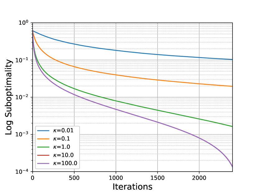
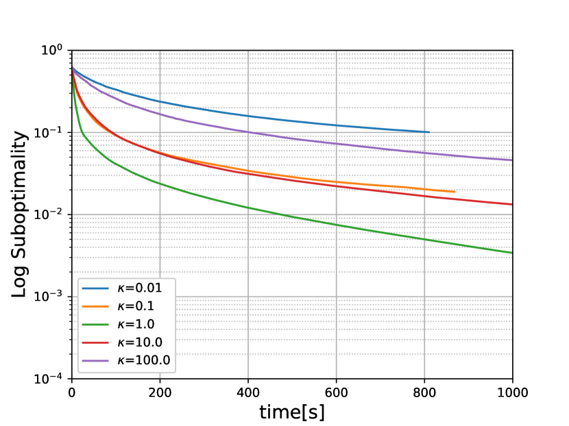
Figure 1: Suboptimality for solving Lasso ($\lambda$=$10^{-6}$) for the RCV1 dataset on a ring of 16 nodes. We illustrate the performance of CoLa: a) number of iterations; b) time. $\kappa$ here denotes the number of local data passes per communication round.

4 Experimental results

Here we illustrate the advantages of CoLa in three respects: firstly we investigate the application in different network topologies and with varying subproblem quality $\Theta$; secondly, we compare CoLa with state-of-the-art decentralized baselines: \footnotesize1⃝, DIGing (Nedic et al., 2017), which generalizes the gradient-tracking technique of the EXTRA algorithm (Shi et al., 2015), and \footnotesize2⃝, Decentralized ADMM (aka. consensus ADMM), which extends the classical ADMM (Alternating Direction Method of Multipliers) method (Boyd et al., 2011) to the decentralized setting (Shi et al., 2014; Wei and Ozdaglar, 2013); Finally, we show that CoLa works in the challenging unreliable network environment where each node has a certain chance to drop out of the network.

We implement all algorithms in PyTorch with MPI backend. The decentralized network topology is simulated by running one thread per graph node, on a $2$$\times$$12$ core Intel Xeon CPU E5-2680 v3 server with 256 GB RAM. Table 1 describes the datasets used in the experiments. For Lasso, the columns of $\mathbf{A}$ are features. For ridge regression, the columns are features and samples for CoLa primal and CoLa dual, respectively. The order of columns is shuffled once before being distributed across the nodes. Due to space limit, details on the experimental configurations are included in Appendix D.

Table 1: Datasets Used for Empirical Study

Dataset	​​#Training	​​#Features	​​Sparsity
URL	2M	3M	3.5e-5
Webspam	350K	16M	2.0e-4
Epsilon	400K	2K	1.0
RCV1 Binary	677K	47K	1.6e-3

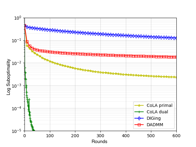
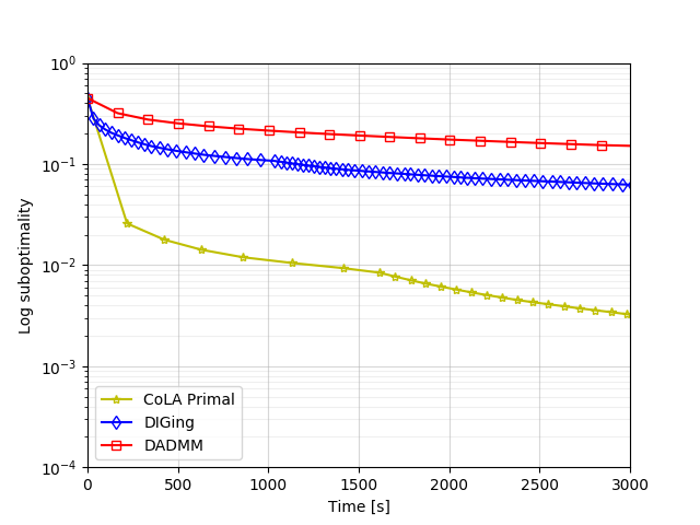
Figure 2: Convergence of CoLa for solving problems on a ring of $K$=$16$ nodes. Left) Ridge regression on URL reputation dataset ($\lambda$=$10^{-4}$); Right) Lasso on webspam dataset ($\lambda$=$10^{-5}$).

Effect of approximation quality $\Theta$. We study the convergence behavior in terms of the approximation quality $\Theta$. Here, $\Theta$ is controlled by the number of data passes $\kappa$ on subproblem (1) per node. Figure 1 shows that increasing $\kappa$ always results in less number of iterations (less communication rounds) for CoLa. However, given a fixed network bandwidth, it leads to a clear trade-off for the overall wall-clock time, showing the cost of both communication and computation. Larger $\kappa$ leads to less communication rounds, however, it also takes more time to solve subproblems. The observations suggest that one can adjust $\Theta$ for each node to handle system heterogeneity, as what we have discussed at the end of LABEL:{sec:cola}.

Effect of graph topology. Fixing $K$=$16$, we test the performance of CoLa on 5 different topologies: ring, 2-connected cycle, 3-connected cycle, 2D grid and complete graph. The mixing matrix $\mathcal{W}$ is given by Metropolis weights for all test cases (details in Appendix B). Convergence curves are plotted in Figure 4. One can observe that for all topologies, CoLa converges monotonically and especailly when all nodes in the network are equal, smaller $\beta$ leads to a faster convergence rate. This is consistent with the intuition that $1-\beta$ measures the connectivity level of the topology.

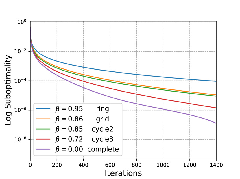
Figure 3: Performance comparison of CoLa on different topologies. Solving Lasso regression ($\lambda$=$10^{-6}$) for RCV1 dataset with $16$ nodes.

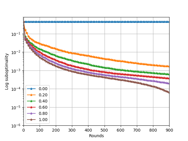
Figure 4: Performance of CoLa when nodes have $p$ chance of staying in the network on the URL dataset ($\lambda$=$10^{-4}$). Freezing $\mathbf{x}_{[k]}$ when node $k$ leaves the network.

Superior performance compared to baselines. We compare CoLa with DIGing and D-ADMM for strongly and general convex problems. For general convex objectives, we use Lasso regression with $\lambda=10^{-4}$ on the webspam dataset; for the strongly convex objective, we use Ridge regression with $\lambda=10^{-5}$ on the URL reputation dataset. For Ridge regression, we can map CoLa to both primal and dual problems. Figure 2 traces the results on log-suboptimality. One can observe that for both generally and strongly convex objectives, CoLa significantly outperforms DIGing and decentralized ADMM in terms of number of communication rounds and computation time. While DIGing and D-ADMM need parameter tuning to ensure convergence and efficiency, CoLa is much easier to deploy as it is parameter free. Additionally, convergence guarantees of ADMM relies on exact subproblem solvers, whereas inexact solver is allowed for CoLa.

Fault tolerance to unreliable nodes. Assume each node of a network only has a chance of $p$ to participate in each round. If a new node $k$ joins the network, then local variables are initialized as $\mathbf{x}_{[k]}=0$; if node  $k$ leaves the network, then $\mathbf{x}_{[k]}$ will be frozen with $\Theta_{k}=1$. All remaining nodes dynamically adjust their weights to maintain the doubly stochastic property of $\mathcal{W}$. We run CoLa on such unreliable networks of different $p$s and show the results in Figure 4. First, one can observe that for all $p>0$ the suboptimality decreases monotonically as CoLa progresses. It is also clear from the result that a smaller dropout rate (a larger $p$) leads to a faster convergence of CoLa.

5 Discussion and conclusions

In this work we have studied training generalized linear models in the fully decentralized setting. We proposed a communication-efficient decentralized framework, termed CoLa, which is free of parameter tuning. We proved that it has a sublinear rate of convergence for general convex problems, allowing e.g. L1 regularizers, and has a linear rate of convergence for strongly convex objectives. Our scheme offers primal-dual certificates which are useful in the decentralized setting. We demonstrated that CoLa offers full adaptivity to heterogenous distributed systems on arbitrary network topologies, and is adaptive to changes in network size and data, and offers fault tolerance and elasticity. Future research directions include improving subproblems, as well as extension to the network topology with directed graphs, as well as recent communication compression schemes (Stich et al., 2018).

Acknowledgments. We thank Prof. Bharat K. Bhargava for fruitful discussions. We acknowledge funding from SNSF grant 200021_175796, Microsoft Research JRC project ‘Coltrain’, as well as a Google Focused Research Award.

Appendix

Appendix A Definitions

Definition 1 ($L$-Lipschitz continuity).

A function $h:{\mathbb{R}}^{n}\rightarrow{\mathbb{R}}$ is $L$-Lipschitz continuous if $\forall\;\mathbf{u},\mathbf{v}\in{\mathbb{R}}^{n}$, it holds that

$$|h(\mathbf{u})-h(\mathbf{v})|\leq L\|\mathbf{u}-\mathbf{v}\|.$$

Definition 2 ($1/\tau$-Smoothness).

A differentiable function $f:{\mathbb{R}}^{n}\rightarrow{\mathbb{R}}$ is $1/\tau$-smooth if its gradient is $1/\tau$-Lipschitz continuous, or equivalently, $\forall~{}\mathbf{u},\mathbf{v}$ it holds

$$\textstyle f(\mathbf{u})\leq f(\mathbf{v})+\langle\nabla f(\mathbf{v}),\mathbf{u}-\mathbf{v}\rangle+\frac{1}{2\tau}\|\mathbf{u}-\mathbf{v}\|^{2}.$$ (11)

Definition 3 ($L$-Bounded support).

The function $g:{\mathbb{R}}^{n}\rightarrow{\mathbb{R}}\cup\{+\infty\}$ has $L$-bounded support if it holds $g(\mathbf{u})<+\infty\Rightarrow\|\mathbf{u}\|\leq L$.

Definition 4 ($\mu$-Strong convexity).

A function $h:{\mathbb{R}}^{n}\rightarrow{\mathbb{R}}$ is $\mu$-strongly convex for $\mu\geq 0$ if $\forall~{}\mathbf{u},\mathbf{v}$, it holds $h(\mathbf{u})\geq h(\mathbf{v})+\langle\mathbf{s},\mathbf{u}-\mathbf{v}\rangle+\frac{\mu}{2}\|\mathbf{u}-\mathbf{v}\|^{2}$, for any $\mathbf{s}\in\partial h(\mathbf{v})$, where $\partial h(\mathbf{v})$ is the subdifferential of $h$ at $\mathbf{v}$.

Lemma 3 (Duality between Lipschitzness and L-Bounded Support).

A generalization of (Rockafellar, 2015, Corollary 13.3.3). Given a proper convex function $g$ it holds that $g$ has $L$-bounded support w.r.t. the norm $\left\lVert{.}\right\rVert$ if and only if $g^{*}$ is $L$-Lipschitz w.r.t. the dual norm $\left\lVert{.}\right\rVert_{*}$.

Appendix B Graph topology

Let $\mathcal{E}$ be the set of edges of a graph. For time-invariant undirected graph the mixing matrix should satisfy the following properties:

1. (Double stochasticity) $\mathcal{W}\mathbf{1}=\mathbf{1}$, $\mathbf{1}^{\top}\mathcal{W}=\mathbf{1}^{\top}$;

2. (Symmetrization) For all $i,j$, $\mathcal{W}_{ij}=\mathcal{W}_{ji}$;

3. (Edge utilization) If $(i,j)\in\mathcal{E}$, then $\mathcal{W}_{ij}>0$; otherwise $\mathcal{W}_{ij}=0$.

A desired mixing matrix can be constructed using Metropolis-Hastings weights (Hastings, 1970):

$$\mathcal{W}_{ij}=\begin{cases}1/(1+\max\{d_{i},d_{j}\}),&\text{if }(i,j)\in\mathcal{E}\\ 0,&\text{if }(i,j)\not\in\mathcal{E}\text{ and }j\neq i\\ 1-\sum_{l\in\mathcal{N}_{i}}\mathcal{W}_{il},&\text{if }j=i,\end{cases}$$

where $d_{i}=|\mathcal{N}_{i}|$ is the degree of node $i$.

Appendix C Proofs

This section consists of three parts. Tools and observations are provided in Section C.1; The main lemmas for the convergence analysis are proved in Section C.2 ; The main theorems and implications are proved in Section C.3.

In some circumstances, it is convenient to use notations of array of stack column vectors. For example, one can stack local estimates $\mathbf{v}_{k}$ to matrix $\mathbf{V}:=[\mathbf{v}_{1};\cdots;\mathbf{v}_{K}]$, $\Delta\mathbf{V}=[\Delta\mathbf{v}_{1};\cdots;\Delta\mathbf{v}_{K}]$. The consensus vector $\mathbf{v}_{c}$ is repeated $K$ times which will be stacked similarly: $\mathbf{V}_{c}:=\mathbf{A}\mathbf{x}\mathbf{1}_{K}^{\top}=\mathbf{V}\mathbf{E}$ where $\mathbf{E}=\frac{1}{K}\mathbf{1}_{K}\mathbf{1}_{K}^{\top}$. The consensus violation under the two notations is written as

$$\textstyle\left\lVert{\mathbf{V}-\mathbf{V}_{c}}\right\rVert_{F}^{2}=\sum_{k=1}^{K}\left\lVert{\mathbf{v}_{k}-\mathbf{A}\mathbf{x}}\right\rVert_{2}^{2}.$$

Then Step 1 in CoLa is equivalent to

$$\mathbf{V}^{(t+1)}=\mathbf{V}^{(t)}\mathcal{W}+\gamma K\Delta\mathbf{V}^{(t)}$$ (12)

Besides, we also adopt following notations in the proof when there is no ambiguity: $\mathbf{v}_{k}^{\prime}:=\sum_{l=1}^{K}\mathcal{W}_{kl}\mathbf{v}_{l}$, $\mathbf{g}_{k}:=\nabla f(\mathbf{v}_{k})$, $\mathbf{g}_{k}^{\prime}:=\nabla f(\mathbf{v}_{k}^{\prime})$ and $\bar{\mathbf{g}}:=\frac{1}{K}\sum_{k=1}^{K}\mathbf{g}_{k}$. For the decentralized duality gap $G_{\mathcal{H}}(\mathbf{x},\{\mathbf{v}_{k}\}_{k=1}^{K},\{\mathbf{w}_{k}\}_{k=1}^{K})$, when $\mathbf{w}_{k}=\nabla f(\mathbf{v}_{k})$, we simplify $G_{\mathcal{H}}(\mathbf{x},\{\mathbf{v}_{k}\}_{k=1}^{K},\{\mathbf{w}_{k}\}_{k=1}^{K})$ to be $G_{\mathcal{H}}(\mathbf{x},\{\mathbf{v}_{k}\}_{k=1}^{K})$ in the sequel.

On a high level, we prove the convergence rates by bounding per-iteration reduction $\mathbb{E}[\mathcal{H}_{A}^{(t)}-\mathcal{H}_{A}^{(t+1)}]$ using decentralized duality gap and other related terms, then try to obtain the final rates by properly using specific properties of the objectives.

However, the specific analysis of the new fully decentralized algorithm CoLa poses many new challenges, and we propose significantly new proof techniques in the analysis. Specifically, i) we introduce the decentralized duality gap, which is suited for the decentralized algorithm CoLa; ii) consensus violation is the usually challenging part in analyzing decentralized algorithms. Unlike using uniform bounds for consensus violations, e.g., (Yuan et al., 2016), we properly combine the consensus violation term and the objective decrease term (c.f. Lemmas 6 and 8), thus reaching arguably tight convergence bounds for both the consensus violation term and the objective.

C.1 Observations and properties

In this subsection we introduce basic lemmas. Lemma 1 establishes the relation between $\{{\bf v}_{k}\}_{k=1}^{K}$ and ${\mathbf{v}_{c}}$ and bounds $F_{A}({\bf x})$ using $\mathcal{H}_{A}({\bf x})$ and the consensus violation.

See 1

Proof of Lemma 1.

Let ${\widetilde{{\bf v}}}:=\frac{1}{K}\sum_{k=1}^{K}\mathbf{v}_{k}$. Using the doubly stochastic property of the matrix $\mathcal{W}$

$$\widetilde{{\bf v}}^{(t+1)} =\frac{1}{K}\sum_{k=1}^{K}{\bf v}_{k}^{(t+1)}=\frac{1}{K}\sum_{k=1}^{K}\left(\sum_{l=1}^{K}\mathcal{W}_{kl}{\bf v}^{(t)}_{l}+\gamma K\Delta{\bf v}_{k}^{(t)}\right)$$

$$=\frac{1}{K}\sum_{l=1}^{K}{\bf v}^{(t)}_{l}+{\gamma}\sum_{k=1}^{K}\Delta{\bf v}_{k}^{(t)}=\widetilde{{\bf v}}^{(t)}+\gamma\sum_{k=1}^{K}\Delta{\bf v}_{k}^{(t)}$$

On the other hand, ${\bf v}_{c}^{(t)}:=\mathbf{A}\mathbf{x}^{(t)}$ is updated based on all changes of local variables $\{{\bf x}_{[k]}\}_{k=1}^{K}$

$${\bf v}_{c}^{(t+1)}={\bf v}_{c}^{(t)}+\gamma\sum_{k=1}^{K}\Delta{\bf v}_{k}^{(t)}.$$

Since $\widetilde{{\bf v}}^{(0)}={\bf v}_{c}^{(0)}$, we can conclude that $\widetilde{{\bf v}}^{(t)}={\bf v}_{c}^{(t)}$ $\forall~{}t$. From convexity of $f$ we know

$$F_{A}({\bf x})=f({\bf v}_{c})+g({\bf x})=f\left(\frac{1}{K}\sum_{k=1}^{K}{\bf v}_{k}\right)+g({\bf x})\leq\frac{1}{K}\sum_{k=1}^{K}f({\bf v}_{k})+g({\bf x})=\mathcal{H}({\bf x})$$

Using $1/\tau$-smoothness of $f$ gives

$$\mathcal{H}_{A}({\bf x})= \frac{1}{K}\sum_{k=1}^{K}f({\bf v}_{k})+g({\bf x})$$

$$\leq \frac{1}{K}\sum_{k=1}^{K}\left(f({\bf v}_{c})+\nabla f({\bf v}_{c})^{\top}({\bf v}_{k}-{\bf v}_{c})+\frac{1}{2\tau}\left\lVert{{\bf v}_{k}-{\bf v}_{c}}\right\rVert^{2}\right)+g({\bf x})$$

$$= F_{A}({\bf x})+\frac{1}{2\tau K}\sum_{k=1}^{K}\left\lVert{{\bf v}_{k}-{\bf v}_{c}}\right\rVert^{2}.$$

∎

The following lemma introduces the dual problem and the duality gap of (DA). See 2

Proof.

Let $\bm{\lambda}_{k}$ be the Lagrangian multiplier for the constraint ${\bf v}_{k}=\mathbf{A}\mathbf{x}$, the Lagrangian function is

$$L(\mathbf{x},\{\mathbf{v}_{k}\}_{k=1}^{K},\{\bm{\lambda}_{k}\}_{k=1}^{K})=\frac{1}{K}\sum_{k=1}^{K}f(\mathbf{v}_{k})+\sum_{i=1}^{n}g_{i}(\mathbf{x}_{i})+\sum_{k=1}^{K}\langle\bm{\lambda}_{k},\mathbf{A}\mathbf{x}-\mathbf{v}_{k}\rangle$$

The dual problem of (DA) follows by taking the infimum with respect to both $\mathbf{x}$ and $\{\mathbf{v}_{k}\}_{k=1}^{K}$:

$$\inf_{\mathbf{x},\{\mathbf{v}_{k}\}_{k=1}^{K}}L(\mathbf{x},\{\mathbf{v}_{k}\}_{k=1}^{K},\{\bm{\lambda}_{k}\}_{k=1}^{K})$$

$$= \inf_{\mathbf{x},\{\mathbf{v}_{k}\}_{k=1}^{K}}\frac{1}{K}\sum_{k=1}^{K}f(\mathbf{v}_{k})+\sum_{i=1}^{n}g_{i}(\mathbf{x}_{i})+\sum_{k=1}^{K}\langle\bm{\lambda}_{k},\mathbf{A}\mathbf{x}-\mathbf{v}_{k}\rangle$$

$$= \sum_{k=1}^{K}\inf_{\{\mathbf{v}_{k}\}_{k=1}^{K}}(\frac{1}{K}f(\mathbf{v}_{k})-\langle\bm{\lambda}_{k},\mathbf{v}_{k}\rangle)+\inf_{\mathbf{x}}(\sum_{i=1}^{n}g_{i}(\mathbf{x}_{i})+\sum_{k=1}^{K}\langle\bm{\lambda}_{k},\mathbf{A}\mathbf{x}\rangle)$$

$$= -\sum_{k=1}^{K}\sup_{\{\mathbf{v}_{k}\}_{k=1}^{K}}(\langle\bm{\lambda}_{k},\mathbf{v}_{k}\rangle-\frac{1}{K}f(\mathbf{v}_{k}))-\sup_{\mathbf{x}}(-\sum_{k=1}^{K}\langle\mathbf{a}_{k},\mathbf{A}\mathbf{x}\rangle-\sum_{i=1}^{n}g_{i}(\mathbf{x}_{i}))$$

$$= -\sum_{k=1}^{K}\frac{1}{K}f^{*}(K\bm{\lambda}_{k})-\sum_{i=1}^{n}g^{*}_{i}(-\sum_{k=1}^{K}\mathbf{A}_{i}^{\top}\bm{\lambda}_{k})$$

Let us change variables from $\bm{\lambda}_{k}$ to $\mathbf{w}_{k}$ by setting $\mathbf{w}_{k}:=K\bm{\lambda}_{k}$. If written in terms of minimization, the Lagrangian dual of $\mathcal{H}_{A}$ is

$$\textstyle\min_{\{\mathbf{w}_{k}\}_{k=1}^{K}}\mathcal{H}_{B}{\{\mathbf{w}_{k}\}_{k=1}^{K}}=\frac{1}{K}\sum_{k=1}^{K}f^{*}(\mathbf{w}_{k})+\sum_{i=1}^{n}g^{*}_{i}\left(-\frac{1}{K}\sum_{k=1}^{K}\mathbf{A}_{i}^{\top}\mathbf{w}_{k}\right)$$ (13)

The optimality condition is that $\mathbf{w}_{k}=\nabla f(\mathbf{v}_{k})$. Now we can see the duality gap is

$$G_{\mathcal{H}}= \mathcal{H}_{A}+\mathcal{H}_{B}$$

$$= \frac{1}{K}\sum_{k=1}^{K}f(\mathbf{v}_{k})+\sum_{i=1}^{n}g_{i}(x_{i})+\frac{1}{K}\sum_{k=1}^{K}f^{*}(\mathbf{w}_{k})+\sum_{i=1}^{n}g^{*}_{i}\left(-\frac{1}{K}\sum_{k=1}^{K}\mathbf{A}_{i}^{\top}\mathbf{w}_{k}\right)$$

∎

The following lemma correlates the consensus violation with the magnitude of the $\mathbf{v}$ parameter updates $\left\lVert{\Delta\mathbf{v}_{k}}\right\rVert_{2}^{2}$.

Lemma 4.

The consensus violation during the execution of Algorithm 1 can be bound by

$$\sum_{k=1}^{K}\left\lVert{\mathbf{v}_{k}^{(t+1)}-\mathbf{A}\mathbf{x}^{(t+1)}}\right\rVert_{2}^{2}\leq\beta\sum_{k=1}^{K}\left\lVert{\mathbf{v}_{k}^{(t)}-\mathbf{A}\mathbf{x}^{(t)}}\right\rVert_{2}^{2}+(1-\beta)c_{1}(\beta,\gamma,K)\sum_{k=1}^{K}\left\lVert{\Delta\mathbf{v}_{k}^{(t)}}\right\rVert_{2}^{2}$$ (14)

where $c_{1}(\beta,\gamma,K):=\gamma^{2}K^{2}/(1-\beta)^{2}$.

Proof.

Consider the norm of consensus violation at time $t+1$ and apply Algo. Step 1

$$\small\left\lVert{\mathbf{V}^{(t+1)}-\mathbf{V}^{(t+1)}_{c}}\right\rVert_{F}^{2}=\left\lVert{\mathbf{V}^{(t+1)}(\mathbf{I}-\mathbf{E})}\right\rVert_{F}^{2}=\left\lVert{(\mathbf{V}^{(t)}\mathcal{W}+\gamma K\Delta\mathbf{V}^{(t)})(\mathbf{I}-\mathbf{E})}\right\rVert_{F}^{2}.$$

Further, use $\mathcal{W}(\mathbf{I}-\mathbf{E})=(\mathbf{I}-\mathbf{E})(\mathcal{W}-\mathbf{E})$, $\left\lVert{\mathbf{I}-\mathbf{E}}\right\rVert_{\infty}=1$, and Young’s inequality with $\varepsilon_{\mathbf{v}}$

$$\left\lVert{\mathbf{V}^{(t+1)}-\mathbf{V}^{(t+1)}_{c}}\right\rVert_{F}^{2}\leq(1+\varepsilon_{\mathbf{v}})\left\lVert{\mathbf{V}^{(t)}(\mathbf{I}-\mathbf{E})(\mathcal{W}-\mathbf{E})}\right\rVert_{F}^{2}+(1+\frac{1}{\varepsilon_{\mathbf{v}}})\gamma^{2}K^{2}\left\lVert{\Delta\mathbf{V}^{(t)}}\right\rVert_{F}^{2}.$$

Use the spectral property of $\mathcal{W}$ we therefore have:

$$\left\lVert{\mathbf{V}^{(t+1)}-\mathbf{V}^{(t+1)}_{c}}\right\rVert_{F}^{2}\leq(1+\varepsilon_{\mathbf{v}})\beta^{2}\left\lVert{\mathbf{V}^{(t)}-\mathbf{V}^{(t)}_{c}}\right\rVert_{F}^{2}+(1+\frac{1}{\varepsilon_{\mathbf{v}}})\gamma^{2}K^{2}\left\lVert{\Delta\mathbf{V}^{(t)}}\right\rVert_{F}^{2}.$$ (15)

Recursively apply (15) for $i=0,\ldots,t-1$ gives

$$\left\lVert{\mathbf{V}^{(t)}-\mathbf{V}^{(t)}_{c}}\right\rVert_{F}^{2}\leq(1+\frac{1}{\varepsilon_{\mathbf{v}}})\gamma^{2}K^{2}\sum_{i=0}^{t-1}((1+\varepsilon_{\mathbf{v}})\beta^{2})^{t-1-i}\left\lVert{\Delta\mathbf{V}^{(i)}}\right\rVert_{F}^{2}.$$ (16)

Consider $\left\lVert{\Delta\mathbf{V}^{(t)}}\right\rVert_{F}^{2}$ generated at time $t$, it will be used in (16) from time $t+1,t+2,\ldots,$ with coefficients $1,(1+\varepsilon_{\mathbf{v}})\beta^{2},((1+\varepsilon_{\mathbf{v}})\beta^{2})^{2},\ldots$. Sum of such coefficients are finite

$$(1+\frac{1}{\varepsilon_{\mathbf{v}}})\gamma^{2}K^{2}\sum_{t=T}^{\infty}((1+\varepsilon_{\mathbf{v}})\beta^{2})^{t-T}\leq\gamma^{2}K^{2}\frac{1+1/\varepsilon_{\mathbf{v}}}{1-(1+\varepsilon_{\mathbf{v}})\beta^{2}}=:c_{1}(\beta,\gamma,K)$$ (17)

where we need $(1+\varepsilon_{\mathbf{v}})\beta^{2}<1$. To minimize $c_{1}(\beta,\gamma,K)$ we can choose $\varepsilon_{\mathbf{v}}=1/\beta-1$

$$c_{1}(\beta,\gamma,K)=\gamma^{2}K^{2}/(1-\beta)^{2}$$ (18)

Then (15) becomes

$$\sum_{k=1}^{K}\left\lVert{\mathbf{v}_{k}^{(t+1)}-\mathbf{A}\mathbf{x}^{(t+1)}}\right\rVert_{2}^{2}\leq\beta\sum_{k=1}^{K}\left\lVert{\mathbf{v}_{k}^{(t)}-\mathbf{A}\mathbf{x}^{(t)}}\right\rVert_{2}^{2}+(1-\beta)c_{1}(\beta,\gamma,K)\sum_{k=1}^{K}\left\lVert{\Delta\mathbf{v}_{k}^{(t)}}\right\rVert_{2}^{2}$$

∎

Lemma 5.

Let $\Delta{{\bf x}^{\star}_{[k]}}$ and $\Delta{{\bf x}_{[k]}}$ be the exact and $\Theta$-inexact solution of subproblem $\mathscr{G}^{\sigma^{\prime}}_{k}({}\cdot{};\mathbf{v}_{k},{\bf x}_{[k]})$. The change of iterates satisfies the following inequality

$$\frac{\sigma^{\prime}}{4\tau}\sum_{k=1}^{K}\left\lVert{\mathbf{A}\Delta\mathbf{x}_{[k]}}\right\rVert_{2}^{2}\leq(1+\Theta)(\mathcal{H}_{A}({\bf 0};\{\mathbf{v}_{k}\})-\mathcal{H}_{A}(\Delta\mathbf{x}^{\star};\{\mathbf{v}_{k}\}))$$ (19)

Proof.

First use the Taylor expansion of $\mathscr{G}^{\sigma^{\prime}}_{k}({}\cdot{};\mathbf{v}_{k},{\bf x}_{[k]})$ and the defnition of $\Delta{{\bf x}^{\star}_{[k]}}$ we have

$$\frac{\sigma^{\prime}}{2\tau}\left\lVert{\mathbf{A}(\Delta\mathbf{z}-\Delta\mathbf{x}^{\star})_{[k]}}\right\rVert_{2}^{2}\leq\mathscr{G}^{\sigma^{\prime}}_{k}\left(\Delta\mathbf{z}_{[k]};\mathbf{v}_{k},{\bf x}_{[k]}\right)-\mathscr{G}^{\sigma^{\prime}}_{k}\left(\Delta{{\bf x}^{\star}_{[k]}};\mathbf{v}_{k},{\bf x}_{[k]}\right)$$ (20)

for all $\Delta\mathbf{z}_{[k]}\in{\mathbb{R}}^{n}$ and $k=1,\ldots,K$. Apply (20) with $\Delta\mathbf{z}_{[k]}={\bf 0}$ for all $k$ and sum them up yields

$$\frac{\sigma^{\prime}}{2\tau}\sum_{k=1}^{K}\left\lVert{\mathbf{A}\Delta\mathbf{x}^{\star}_{[k]}}\right\rVert_{2}^{2}\leq\mathcal{H}_{A}({\bf 0};\{\mathbf{v}_{k}\})-\mathcal{H}_{A}(\Delta\mathbf{x}^{\star};\{\mathbf{v}_{k}\})$$ (21)

Similarly, apply (20) for $\Delta\mathbf{z}_{[k]}=\Delta\mathbf{x}_{[k]}$ for all $k$ and sum them up gives

$$\frac{\sigma^{\prime}}{2\tau}\sum_{k=1}^{K}\left\lVert{\mathbf{A}(\Delta\mathbf{x}-\Delta\mathbf{x}^{\star})_{[k]}}\right\rVert_{2}^{2}\leq\mathcal{H}_{A}(\Delta\mathbf{x};\{\mathbf{v}_{k}\})-\mathcal{H}_{A}(\Delta\mathbf{x}^{\star};\{\mathbf{v}_{k}\})$$ (22)

By Assumption 1 the previous inequality becomes

$$\frac{\sigma^{\prime}}{2\tau}\sum_{k=1}^{K}\left\lVert{\mathbf{A}(\Delta\mathbf{x}-\Delta\mathbf{x}^{\star})_{[k]}}\right\rVert_{2}^{2}\leq\Theta(\mathcal{H}_{A}({\bf 0};\{\mathbf{v}_{k}\})-\mathcal{H}_{A}(\Delta\mathbf{x}^{\star};\{\mathbf{v}_{k}\}))$$ (23)

The following inequality is straightforward

$$\frac{1}{2}\sum_{k=1}^{K}\left\lVert{\mathbf{A}\Delta\mathbf{x}_{[k]}}\right\rVert_{2}^{2}\leq\sum_{k=1}^{K}\left\lVert{\mathbf{A}\Delta\mathbf{x}^{\star}_{[k]}}\right\rVert_{2}^{2}+\sum_{k=1}^{K}\left\lVert{\mathbf{A}(\Delta\mathbf{x}-\Delta\mathbf{x}^{\star})_{[k]}}\right\rVert_{2}^{2}$$ (24)

Multiply (24) with $\sigma^{\prime}/(2\tau)$ and use (21) and (23)

$$\frac{\sigma^{\prime}}{4\tau}\sum_{k=1}^{K}\left\lVert{\mathbf{A}\Delta\mathbf{x}_{[k]}}\right\rVert_{2}^{2}\leq(1+\Theta)(\mathcal{H}_{A}({\bf 0};\{\mathbf{v}_{k}\})-\mathcal{H}_{A}(\Delta\mathbf{x}^{\star};\{\mathbf{v}_{k}\}))$$ (25)

∎

C.2 Main lemmas

We first present two main lemmas for the per-iteration improvement.

Lemma 6.

Let $g_{i}$ be strongly convex with convexity parameter $\mu_{g}\geq 0$ with respect to the norm $\left\lVert{\cdot}\right\rVert,\forall~{}i\in[n]$. Then for all iterations $t$ of outer loop, and any $s\in[0,1]$, it holds that

$$\begin{split}&\mathbb{E}\left[\mathcal{H}_{A}(\mathbf{x}^{(t)};\mathbf{v}_{k}^{(t)})-\mathcal{H}_{A}(\mathbf{x}^{(t+1)};\mathbf{v}_{k}^{(t+1)})-\alpha\frac{\gamma\sigma_{1}^{\prime}}{2\tau}\sum_{k=1}^{K}\left\lVert{\mathbf{A}\Delta\mathbf{x}_{[k]}^{(t)}}\right\rVert_{2}^{2}\right]\\ \geq&\eta\left(sG_{\mathcal{H}}({\bf x}^{(t)};\{{\mathbf{v}_{k}^{\prime(t)}}\}_{k=1}^{K})-\frac{s^{2}\bar{\sigma}^{\prime}}{2\tau}R^{(t)}\right)-\frac{9\beta\eta}{2\tau\sigma^{\prime}}\sum_{k=1}^{K}\left\lVert{\mathbf{v}_{k}^{(t)}-\mathbf{A}\mathbf{x}^{(t)}}\right\rVert_{2}^{2}\end{split}$$ (26)

where $\alpha\in[0,1]$ is a constant and $\eta:=\gamma(1-\Theta)(1-\alpha)$ and $\sigma_{1}^{\prime}:=\frac{(1-\Theta)}{2(1+\Theta)}\sigma^{\prime}$ and $\bar{\sigma}^{\prime}:=(1+\beta)\sigma^{\prime}$ and $\mathbf{v}_{k}^{\prime}:=\sum_{l=1}^{K}\mathcal{W}_{kl}\mathbf{v}_{l}$.

$$\textstyle R^{(t)}:=-\frac{\tau\mu_{g}(1-s)}{\bar{\sigma}^{\prime}s}\left\lVert{{\bf u}^{(t)}-{\bf x}^{(t)}}\right\rVert^{2}+\sum_{k=1}^{K}\left\lVert{\mathbf{A}({\bf u}^{(t)}-{\bf x}^{(t)})_{[k]}}\right\rVert^{2}$$ (27)

for ${\bf u}^{(t)}\in{\mathbb{R}}^{n}$ with $\bar{\mathbf{g}}^{\prime(t)}:=\frac{1}{K}\sum_{k=1}^{K}\nabla f(\mathbf{v}_{k}^{\prime(t)})$

$$u_{i}^{(t)}\in\partial g_{i}^{*}(-\mathbf{A}_{i}^{\top}\bar{\mathbf{g}}^{\prime(t)})\qquad k\text{ s.t. }i\in\mathcal{P}_{k}$$ (28)

Proof of Lemma 6.

For simplicity, we write $\mathcal{H}_{A}^{(t)}$ instead of $\mathcal{H}_{A}(\mathbf{x}^{(t)};\{\mathbf{v}_{k}^{(t)}\}_{k=1}^{K})$ and $\mathbf{v}_{k}^{\prime}:=\sum_{i=1}^{K}\mathcal{W}_{ik}\mathbf{v}_{i}$.

$$\mathbb{E}[\mathcal{H}_{A}^{(t)}-\mathcal{H}_{A}^{(t+1)}]$$

$$= \frac{1}{K}\sum_{k=1}^{K}f({{{\bf v}_{k}}})-\frac{1}{K}\sum_{k=1}^{K}f\left(\mathbf{v}_{k}^{\prime}+\gamma K\Delta{\bf v}_{[k]}\right)+g({\bf x})-g({\bf x}+\gamma\Delta{\bf x})$$

$$= \underbrace{\frac{1}{K}\sum_{k=1}^{K}f({{{\bf v}_{k}}})-\frac{1}{K}\sum_{k=1}^{K}f\left(\mathbf{v}_{k}^{\prime}\right)}_{D_{1}}$$

$$+\underbrace{\sum_{k=1}^{K}\left\{\frac{1}{K}f\left(\mathbf{v}_{k}^{\prime}\right)+g({\bf x}_{[k]})\right\}-\sum_{k=1}^{K}\left\{\frac{1}{K}f\left(\mathbf{v}_{k}^{\prime}+\gamma K\Delta{\bf v}_{[k]}\right)+g({\bf x}_{[k]}+\gamma\Delta{\bf x}_{[k]})\right\}}_{D_{2}}$$

By the convexity of $f$, $D_{1}\geq 0$. Using the convexity of $f$ and $g$ in $D_{2}$ we have

$$\frac{1}{\gamma}D_{2}\geq \sum_{k=1}^{K}\left\{\frac{1}{K}f\left(\mathbf{v}_{k}^{\prime}\right)+g({\bf x}_{[k]})\right\}-\sum_{k=1}^{K}\left\{\frac{1}{K}f\left(\mathbf{v}_{k}^{\prime}+K\Delta{\bf v}_{[k]}\right)+g({\bf x}_{[k]}+\Delta{\bf x}_{[k]})\right\}$$

$$\geq \mathbb{E}\left[\sum_{k=1}^{K}\mathscr{G}^{\sigma^{\prime}}_{k}\left({\bf 0};\mathbf{v}_{k}^{\prime},{\bf x}_{[k]}\right)-\sum_{k=1}^{K}\mathscr{G}^{\sigma^{\prime}}_{k}\left(\Delta{{\bf x}_{[k]}};\mathbf{v}_{k}^{\prime},{\bf x}_{[k]}\right)\right]$$

Use the Assumption 1 we have

$$D_{2}\geq \gamma\mathbb{E}\left[\sum_{k=1}^{K}\mathscr{G}^{\sigma^{\prime}}_{k}\left({\bf 0};\mathbf{v}_{k}^{\prime},{\bf x}_{[k]}\right)-\sum_{k=1}^{K}\mathscr{G}^{\sigma^{\prime}}_{k}\left(\Delta{{\bf x}_{[k]}};\mathbf{v}_{k}^{\prime},{\bf x}_{[k]}\right)\right]$$

$$\geq \gamma(1-\Theta)\underbrace{\sum_{k=1}^{K}\left\{\mathscr{G}^{\sigma_{2}^{\prime}}_{k}\left({\bf 0};\mathbf{v}_{k}^{\prime},{\bf x}_{[k]}\right)-\mathscr{G}^{\sigma_{2}^{\prime}}_{k}\left(\Delta{{\bf x}_{[k]}^{\star}};\mathbf{v}_{k}^{\prime},{\bf x}_{[k]}\right)\right\}}_{C}$$

Let $\alpha\in[0,1]$ and apply Lemma 5, the previous inequality becomes

$$D_{2}\geq\gamma(1-\Theta)(1-\alpha)C+\alpha\frac{\gamma\sigma_{1}^{\prime}}{2\tau}\sum_{k=1}^{K}\left\lVert{\mathbf{A}\Delta\mathbf{x}_{[k]}}\right\rVert_{2}^{2}$$ (29)

where $\sigma_{1}^{\prime}:=\frac{(1-\Theta)}{2(1+\Theta)}\sigma^{\prime}$. From the definition of $u_{i}$ we know

$$g_{i}(u_{i})=u_{i}(-\mathbf{A}_{i}^{\top}\bar{\mathbf{g}}^{\prime})-g_{i}^{*}(-\mathbf{A}_{i}^{\top}\bar{\mathbf{g}}^{\prime})$$ (30)

Replacing $\Delta{\bf x}_{i}=s(u_{i}-x_{i})$ in $C$ gives

$$C\geq \sum_{k=1}^{K}\left\{\sum_{i\in\mathcal{P}_{k}}(g_{i}(x_{i})-g_{i}(x_{i}+\Delta x_{i}))-\left\langle\mathbf{g}_{k}^{\prime},\mathbf{A}\Delta{\bf x}_{[k]}\right\rangle-\frac{\sigma^{\prime}}{2\tau}\left\lVert{\mathbf{A}\Delta{\bf x}_{[k]}}\right\rVert^{2}\right\}$$

$$\geq \sum_{k=1}^{K}\left\{\sum_{i\in\mathcal{P}_{k}}(sg_{i}(x_{i})-sg_{i}(u_{i})+\frac{\mu_{g}}{2\tau}(1-s)s(u_{i}-x_{i})^{2})-\left\langle\mathbf{g}_{k}^{\prime},\mathbf{A}\Delta{\bf x}_{[k]}\right\rangle-\frac{\sigma^{\prime}}{2\tau}\left\lVert{\mathbf{A}\Delta{\bf x}_{[k]}}\right\rVert^{2}\right\}$$

$$\stackrel{{\scriptstyle\eqref{eq:dual:u}}}{{=}} \sum_{k=1}^{K}(\sum_{i\in\mathcal{P}_{k}}\left(sg_{i}(x_{i})+sg^{*}_{i}(-\mathbf{A}_{i}^{\top}\bar{\mathbf{g}}^{\prime}))+s\langle\mathbf{v}_{k}/K,\mathbf{g}_{k}^{\prime}\rangle\right)-s\sum_{k=1}^{K}(\langle\mathbf{v}_{k}/K,\mathbf{g}_{k}^{\prime}\rangle-\langle\mathbf{A}\mathbf{u}_{[k]},\bar{\mathbf{g}}^{\prime}\rangle)$$

$$+\sum_{k=1}^{K}\sum_{i\in\mathcal{P}_{k}}\left\{\frac{\mu_{g}}{2\tau}(1-s)s(u_{i}-x_{i})^{2}\right\}-\sum_{k=1}^{K}\left\langle\mathbf{g}_{k}^{\prime},\mathbf{A}\Delta{\bf x}_{[k]}\right\rangle-\sum_{k=1}^{K}\frac{\sigma^{\prime}}{2\tau}\left\lVert{\mathbf{A}\Delta{\bf x}_{[k]}}\right\rVert^{2}$$

$$= \sum_{k=1}^{K}\big{\{}\sum_{i\in\mathcal{P}_{k}}\left(sg_{i}(x_{i})+sg^{*}_{i}(-\mathbf{A}_{i}^{\top}\bar{\mathbf{g}}^{\prime})\right)+s\langle\mathbf{v}_{k}/K,{\mathbf{g}}_{k}^{\prime}\rangle\big{\}}+\frac{\mu_{g}}{2}(1-s)s\left\lVert{{\bf u}-{\bf x}}\right\rVert^{2}$$

$$-\sum_{k=1}^{K}\frac{s^{2}\sigma^{\prime}}{2\tau}\left\lVert{\mathbf{A}({\bf u}-{\bf x})_{[k]}}\right\rVert^{2}-s\sum_{k=1}^{K}(\langle\mathbf{v}_{k}/K,\mathbf{g}_{k}^{\prime}\rangle-\langle\mathbf{A}\mathbf{u}_{[k]},\bar{\mathbf{g}}^{\prime}\rangle+\langle\mathbf{g}_{k}^{\prime},\mathbf{A}(\mathbf{u}-\mathbf{x})_{[k]}\rangle)$$

$$= sG_{\mathcal{H}}({\bf x};\{{\mathbf{v}_{k}^{\prime}}\}_{k=1}^{K})+\frac{\mu_{g}}{2}(1-s)s\left\lVert{{\bf u}-{\bf x}}\right\rVert^{2}$$

$$-\frac{s^{2}\sigma^{\prime}}{2\tau}\sum_{k=1}^{K}\left\lVert{\mathbf{A}({\bf u}-{\bf x})_{[k]}}\right\rVert^{2}-s\sum_{k=1}^{K}(\langle\mathbf{v}_{k}^{\prime}/K,\mathbf{g}_{k}^{\prime}\rangle-\langle\mathbf{A}\mathbf{u}_{[k]},\bar{\mathbf{g}}^{\prime}\rangle+\langle\mathbf{g}_{k}^{\prime},\mathbf{A}(\mathbf{u}-\mathbf{x})_{[k]}\rangle)$$

We can bound the last term of the previous equation as $D_{3}$

$$\frac{1}{s}D_{3}= \sum_{k=1}^{K}(\langle\mathbf{v}_{k}^{\prime}/K,\mathbf{g}_{k}^{\prime}\rangle-\langle\mathbf{A}\mathbf{u}_{[k]},\bar{\mathbf{g}}^{\prime}\rangle+\langle\mathbf{g}_{k}^{\prime},\mathbf{A}(\mathbf{u}-\mathbf{x})_{[k]}\rangle)$$

$$= \sum_{k=1}^{K}(\langle\mathbf{g}_{k}^{\prime},\mathbf{v}_{k}^{\prime}/K\rangle-\langle\mathbf{g}_{k}^{\prime},\mathbf{A}\mathbf{u}/K\rangle+\langle\mathbf{g}_{k}^{\prime},\mathbf{A}(\mathbf{u}-\mathbf{x})_{[k]}\rangle)$$

$$= \frac{1}{K}\sum_{k=1}^{K}\langle\mathbf{g}_{k}^{\prime},\mathbf{v}_{k}^{\prime}-\mathbf{A}\mathbf{x}\rangle-\sum_{k=1}^{K}\langle\bar{\mathbf{g}}^{\prime},\mathbf{A}(\mathbf{u}-\mathbf{x})_{[k]}\rangle+\sum_{k=1}^{K}\langle\mathbf{g}_{k}^{\prime},\mathbf{A}(\mathbf{u}-\mathbf{x})_{[k]}\rangle$$

$$= \frac{1}{K}\sum_{k=1}^{K}\langle\mathbf{g}_{k}^{\prime}-\bar{\mathbf{g}}^{\prime},\mathbf{v}_{k}^{\prime}-\mathbf{A}\mathbf{x}\rangle+\sum_{k=1}^{K}\langle\mathbf{g}_{k}^{\prime}-\bar{\mathbf{g}}^{\prime},\mathbf{A}(\mathbf{u}-\mathbf{x})_{[k]}\rangle$$

Bound the gradient terms with consensus violation. First bound $\sum_{k=1}^{K}\left\lVert{\mathbf{g}_{k}^{\prime}-\bar{\mathbf{g}}^{\prime}}\right\rVert_{2}^{2}$, define $\mathbf{g}_{c}:=\nabla f(\mathbf{A}\mathbf{x})$

$$\sum_{k=1}^{K}\left\lVert{\mathbf{g}_{k}^{\prime}-\bar{\mathbf{g}}^{\prime}}\right\rVert_{2}^{2}\leq 2\sum_{k=1}^{K}\left(\left\lVert{\mathbf{g}_{k}^{\prime}-\mathbf{g}_{c}}\right\rVert_{2}^{2}+\left\lVert{\mathbf{g}_{c}-\bar{\mathbf{g}}^{\prime}}\right\rVert_{2}^{2}\right)\leq 2\sum_{k=1}^{K}\left\lVert{\mathbf{g}_{k}^{\prime}-\mathbf{g}_{c}}\right\rVert_{2}^{2}+2\frac{1}{K}\sum_{k=1}^{K}\left\lVert{\mathbf{g}_{c}-{\mathbf{g}}_{k}^{\prime}}\right\rVert_{2}^{2}$$

Apply the $1/\tau$-smoothness of $f$ we have

$$\sum_{k=1}^{K}\left\lVert{\mathbf{g}_{k}^{\prime}-\bar{\mathbf{g}}^{\prime}}\right\rVert_{2}^{2}\leq\frac{4}{\tau^{2}}\sum_{k=1}^{K}\left\lVert{\mathbf{v}_{k}^{\prime}-\mathbf{A}\mathbf{x}}\right\rVert_{2}^{2}\leq\frac{4\beta^{2}}{\tau^{2}}\sum_{k=1}^{K}\left\lVert{\mathbf{v}_{k}-\mathbf{A}\mathbf{x}}\right\rVert_{2}^{2}$$ (31)

Bound the first term in $D_{3}$

$$s\frac{1}{K}\sum_{k=1}^{K}\langle\mathbf{g}_{k}^{\prime}-\bar{\mathbf{g}}^{\prime},\mathbf{v}_{k}^{\prime}-\mathbf{A}\mathbf{x}\rangle\leq \frac{s}{2K}\sum_{k=1}^{K}\left(\tau\left\lVert{\mathbf{g}_{k}^{\prime}-\bar{\mathbf{g}}^{\prime}}\right\rVert_{2}^{2}+\frac{1}{\tau}\left\lVert{\mathbf{v}_{k}^{\prime}-\mathbf{A}\mathbf{x}}\right\rVert_{2}^{2}\right)$$

$$\stackrel{{\scriptstyle\eqref{eq:sum_of_subproblems_reductionNewGH_CV:1}}}{{\leq}} \frac{5\beta^{2}s}{2\tau K}\sum_{k=1}^{K}\left\lVert{\mathbf{v}_{k}-\mathbf{A}\mathbf{x}}\right\rVert_{2}^{2}$$

Bound the second term in $D_{3}$

$$s\sum_{k=1}^{K}\langle\mathbf{g}_{k}^{\prime}-\bar{\mathbf{g}}^{\prime},\mathbf{A}(\mathbf{u}-\mathbf{x})_{[k]}\rangle\leq\frac{\tau}{2\sigma^{\prime}\beta}\sum_{k=1}^{K}\left\lVert{\mathbf{g}_{k}^{\prime}-\bar{\mathbf{g}}^{\prime}}\right\rVert_{2}^{2}+\frac{s^{2}\sigma^{\prime}\beta}{2\tau}\sum_{k=1}^{K}\left\lVert{\mathbf{A}(\mathbf{u}-\mathbf{x})_{[k]}}\right\rVert_{2}^{2}$$

$$\stackrel{{\scriptstyle\eqref{eq:sum_of_subproblems_reductionNewGH_CV:1}}}{{\leq}} \frac{4\beta}{2\tau\sigma^{\prime}}\sum_{k=1}^{K}\left\lVert{\mathbf{v}_{k}-\mathbf{A}\mathbf{x}}\right\rVert_{2}^{2}+\frac{s^{2}\sigma^{\prime}\beta}{2\tau}\sum_{k=1}^{K}\left\lVert{\mathbf{A}(\mathbf{u}-\mathbf{x})_{[k]}}\right\rVert_{2}^{2}$$

Then

$$C\geq sG_{\mathcal{H}}(\mathbf{x},\{\mathbf{v}_{k}^{\prime}\}_{k=1}^{K})+\frac{\mu_{g}}{2}(1-s)s\left\lVert{{\bf u}-{\bf x}}\right\rVert^{2}-\frac{s^{2}(\sigma^{\prime}+\beta\sigma^{\prime})}{2\tau}\sum_{k=1}^{K}\left\lVert{\mathbf{A}({\bf u}-{\bf x})_{[k]}}\right\rVert^{2}$$

$$-\frac{9\beta}{2\tau\sigma^{\prime}}\sum_{k=1}^{K}\left\lVert{\mathbf{v}_{k}-\mathbf{A}\mathbf{x}}\right\rVert_{2}^{2}$$

Then let $\bar{\sigma}^{\prime}:=(1+\beta)\sigma^{\prime}$ and $\eta:=\gamma(1-\Theta)(1-\alpha)$ we have

$$\mathbb{E}[\mathcal{H}_{A}^{(t)}-\mathcal{H}_{A}^{(t+1)}-\alpha\frac{\gamma\sigma_{1}^{\prime}}{2\tau}\sum_{k=1}^{K}\left\lVert{\mathbf{A}\Delta\mathbf{x}_{[k]}^{(t)}}\right\rVert_{2}^{2}]$$

$$\geq \eta\left(sG_{\mathcal{H}}({\bf x}^{(t)};\{{\mathbf{v}_{k}^{\prime(t)}}\}_{k=1}^{K})-\frac{s^{2}\bar{\sigma}^{\prime}}{2\tau}R^{(t)}\right)-\frac{9\eta\beta}{2\tau\sigma^{\prime}}\sum_{k=1}^{K}\left\lVert{\mathbf{v}_{k}^{(t)}-\mathbf{A}\mathbf{x}^{(t)}}\right\rVert_{2}^{2}$$

∎

The following lemma correlates the consensus violation with the size of updates

Lemma 7.

Let $c>0$ be any constant value. Define $\delta^{(0)}:={\bf 0}$ and

$$\delta^{(t+1)}:=\beta\delta^{(t)}+cc_{1}\sum_{k=1}^{K}\left\lVert{\Delta\mathbf{v}^{(t)}_{k}}\right\rVert_{2}^{2}$$ (32)

Then the consensus violation has an upper bound.

$$\sum_{k=1}^{K}\left\lVert{\mathbf{v}^{(t)}_{k}-\mathbf{v}^{(t)}}\right\rVert_{2}^{2}\leq e_{1}\delta^{(t)}$$ (33)

where $e_{1}:=(1-\beta)/c$.

Proof.

Let

$$a_{t}:=\sum_{k=1}^{K}\left\lVert{\Delta\mathbf{v}^{(t)}_{k}}\right\rVert_{2}^{2},b_{t}:=\sum_{k=1}^{K}\left\lVert{\mathbf{v}^{(t)}_{k}-\mathbf{v}^{(t)}}\right\rVert_{2}^{2}$$ (34)

We want to prove that

$$b_{t}\leq e_{1}\delta^{(t)}$$ (35)

First $t=0$, $b_{0}=\delta^{(0)}=0$. If the claim holds for time $t-1$, then $b_{t-1}\leq e_{1}\delta^{(t-1)}$. At time $t$, we have

$$b_{t}\stackrel{{\scriptstyle\eqref{eq:consensus_violation}}}{{\leq}} \beta b_{t-1}+(1-\beta)c_{1}a_{t-1}$$ (36)

$$\leq \beta\frac{1-\beta}{c}\delta^{(t-1)}+(1-\beta)c_{1}a_{t-1}$$ (37)

$$\leq \frac{1-\beta}{c}(\beta\delta^{(t-1)}+cc_{1}a_{t-1})$$ (38)

$$\stackrel{{\scriptstyle\eqref{eq:relate_cv_with_updates:1}}}{{\leq}} e_{1}\delta^{(t)}$$ (39)

Thus we proved the lemma. ∎

Lemma 8.

Let $g_{i}$ be strongly convex with convexity parameter $\mu_{g}\geq 0$ with respect to the norm $\left\lVert{\cdot}\right\rVert,\forall~{}i\in[n]$. Then for all iterations $t$ of outer loop, and $s\in[0,1]$, it holds that

$$\begin{split}&\mathbb{E}[\mathcal{H}_{A}(\mathbf{x}^{(t)};\{\mathbf{v}_{k}^{(t)}\}_{k=1}^{K})-\mathcal{H}_{A}(\mathbf{x}^{(t+1)};\{\mathbf{v}_{k}^{(t+1)}\}_{k=1}^{K})+\frac{1+\beta}{2}\delta^{(t)}-\delta^{(t+1)}]\\ \geq&\eta\left(sG_{\mathcal{H}}(\mathbf{x}^{(t)};\{\textstyle\sum_{i=1}^{K}\mathcal{W}_{ki}\mathbf{v}_{i}^{(t)}\}_{k=1}^{K})-\frac{s^{2}\bar{\sigma}^{\prime}}{2\tau}R^{(t)}\right)\end{split}$$ (40)

where $\alpha:=(1+\frac{(1-\beta)^{2}}{36(1+\Theta)\beta})^{-1}\in[0,1]$, $\eta:=\gamma(1-\Theta)(1-\alpha)$, $\bar{\sigma}^{\prime}:=(1+\beta)\sigma^{\prime}$ and

$$\textstyle R^{(t)}:=-\frac{\tau\mu_{g}(1-s)}{\bar{\sigma}^{\prime}s}\left\lVert{{\bf u}^{(t)}-{\bf x}^{(t)}}\right\rVert^{2}+\sum_{k=1}^{K}\left\lVert{\mathbf{A}({\bf u}^{(t)}-{\bf x}^{(t)})_{[k]}}\right\rVert^{2}$$ (41)

for ${\bf u}^{(t)}\in{\mathbb{R}}^{n}$ with $\bar{\mathbf{g}}^{\prime(t)}:=\sum_{k=1}^{K}\nabla f(\sum_{i=1}^{K}\mathcal{W}_{ik}\mathbf{v}_{i}^{(t)})$

$$u_{i}^{(t)}\in\partial g_{i}^{*}(-\mathbf{A}_{i}^{\top}\bar{\mathbf{g}}^{\prime(t)})\qquad k\text{ s.t. }i\in\mathcal{P}_{k}.$$ (42)

where $\delta^{(t)}$ is defined in Lemma 7.

Proof.

In this proof we use $\mathbf{v}_{k}^{\prime}:=\sum_{i}\mathcal{W}_{ki}\mathbf{v}_{i}$. From Lemma 6 we know that

$$\mathbb{E}\bigg{[}\mathcal{H}_{A}^{(t)}-\mathcal{H}_{A}^{(t+1)}-\alpha\frac{\gamma\sigma_{1}^{\prime}}{2\tau}\sum_{k=1}^{K}\left\lVert{\mathbf{A}\Delta\mathbf{x}_{[k]}^{(t)}}\right\rVert_{2}^{2}+\frac{9\eta\beta}{2\tau\sigma^{\prime}}\sum_{k=1}^{K}\left\lVert{\mathbf{v}_{k}^{(t)}-\mathbf{A}\mathbf{x}^{(t)}}\right\rVert_{2}^{2}\bigg{]}$$

$$\geq \eta\left(sG_{\mathcal{H}}({\bf x}^{(t)};\{{\mathbf{v}_{k}^{\prime(t)}}\}_{k=1}^{K})-\frac{s^{2}\bar{\sigma}^{\prime}}{2\tau}R^{(t)}\right)$$

Use the following notations to simplify the calculation

$$a_{t}:=\sum_{k=1}^{K}\left\lVert{\Delta\mathbf{v}^{(t)}_{k}}\right\rVert_{2}^{2},b_{t}:=\sum_{k=1}^{K}\left\lVert{\mathbf{v}^{(t)}_{k}-\mathbf{v}^{(t)}}\right\rVert_{2}^{2},f_{1}:=\alpha\frac{\gamma\sigma_{1}^{\prime}}{2\tau},f_{2}:=\frac{9\eta\beta}{2\tau\sigma^{\prime}}$$ (43)

From Lemma 7 we know that

$$f_{2}b_{t}-f_{1}a_{t}\leq f_{2}e_{1}\delta^{(t)}-f_{1}(\delta^{(t+1)}-\beta\delta^{(t)})/(cc_{1})=(f_{2}e_{1}+\frac{f_{1}\beta}{cc_{1}})\delta^{(t)}-\frac{f_{1}}{cc_{1}}\delta^{(t+1)}$$ (44)

Fix constant $c$ such that $\frac{f_{1}}{cc_{1}}=1$ in (44)

$$c=\frac{f_{1}}{c_{1}}=\alpha\frac{(1-\beta)^{2}\sigma_{1}^{\prime}}{2\tau\gamma K^{2}}$$ (45)

Fix $(f_{2}e_{1}+\frac{f_{1}\beta}{cc_{1}})=\frac{1+\beta}{2}<1$ in (44), to determine $\alpha\in[0,1]$. First consider $f_{2}e_{1}$

$$f_{2}e_{1}=\frac{9\gamma(1-\Theta)(1-\alpha)\beta}{2\tau\sigma^{\prime}}\frac{1-\beta}{c}\stackrel{{\scriptstyle\eqref{eq:sum_of_subproblems_reductionNew_R1:2}}}{{=}}\frac{1-\alpha}{\alpha}\frac{9(1-\Theta)\beta}{1-\beta}\frac{\gamma K}{\sigma_{1}^{\prime}}$$ (46)

Then we have

$$f_{2}e_{1}+\frac{f_{1}\beta}{cc_{1}}=\frac{1-\alpha}{\alpha}\frac{9(1-\Theta)\beta}{1-\beta}\frac{\gamma K}{\sigma_{1}^{\prime}}+\beta=\frac{1+\beta}{2}<1.$$ (47)

Thus we can fix $\alpha\in[0,1]$ to be

$$\alpha:=\bigg{(}1+\frac{(1-\beta)^{2}}{36(1+\Theta)\beta}\bigg{)}^{-1}$$ (48)

So when have these information.

$$f_{2}b_{t}-f_{1}a_{t}\leq\frac{1+\beta}{2}\delta^{(t)}-\delta^{(t+1)}$$ (49)

Finally, using all of the previous equations we know

$$\mathbb{E}\bigg{[}\mathcal{H}_{A}^{(t)}-\mathcal{H}_{A}^{(t+1)}+\frac{1+\beta}{2}\delta^{(t)}-\delta^{(t+1)}\bigg{]}\geq\eta\left(sG_{\mathcal{H}}({\bf x}^{(t)};\{{\mathbf{v}_{k}^{\prime(t)}}\}_{k=1}^{K})-\frac{s^{2}\bar{\sigma}^{\prime}}{2\tau}R^{(t)}\right)$$ (50)

∎

C.3 Main theorems

Here we present the proofs of Theorem 1 and Theorem 2.

Lemma 9.

If $g_{i}^{*}$ are $L$-Lipschitz continuous for all $i\in[n]$, then

$$\forall~{}t:R^{(t)}\leq 4L^{2}\sum_{k=1}^{K}\sigma_{k}n_{k}=4L^{2}\sigma,$$ (51)

where $\sigma_{k}:=\max_{{\bf x}_{[k]}\in{\mathbb{R}}^{n}}\left\lVert{\mathbf{A}_{[k]}{\bf x}_{[k]}}\right\rVert^{2}/\left\lVert{{\bf x}_{[k]}}\right\rVert^{2}$.

Proof.

For general convex functions, the strong convexity parameter is $\mu_{g}=0$, and hence the definition (41) of the complexity constant $R^{(t)}$ becomes

$$R^{(t)}=\sum_{k=1}^{K}\left\lVert{\mathbf{A}(\mathbf{u}^{(t)}-{\bf x}^{(t)})_{[k]}}\right\rVert^{2}=\sum_{k=1}^{K}\sigma_{k}\left\lVert{(\mathbf{u}^{(t)}-{\bf x}^{(t)})_{[k]}}\right\rVert^{2}\leq\sum_{k=1}^{K}\sigma_{k}|\mathcal{P}_{k}|4L^{2}=4L^{2}\sigma$$

Here the last inequality follows from $L$-Lipschitz property of $g^{*}$. ∎

See 1

Proof.

If $g_{i}(\cdot)$ are $\mu_{g}$-strongly convex, one can use the definition of $\sigma_{k}$ and $\sigma_{\text{max}}$ to find

$$R^{(t)}\leq -\frac{\tau\mu_{g}(1-s)}{\bar{\sigma}^{\prime}s}\left\lVert{{\bf u}^{(t)}-{\bf x}^{(t)}}\right\rVert^{2}+\sum_{k=1}^{K}\left\lVert{\mathbf{A}({\bf u}^{(t)}-{\bf x}^{(t)})_{[k]}}\right\rVert^{2}$$

$$\leq \left(-\frac{\tau\mu_{g}(1-s)}{\bar{\sigma}^{\prime}s}+\sigma_{\text{max}}\right)\left\lVert{{\bf u}^{(t)}-{\bf x}^{(t)}}\right\rVert^{2}.$$ (52)

If we set

$$s_{0}=\frac{\tau\mu_{g}}{\tau\mu_{g}+\sigma_{\text{max}}\bar{\sigma}^{\prime}}$$ (53)

then $R^{(t)}\leq 0$. The duality gap has a lower bound duality gap

$$G_{\mathcal{H}}(\mathbf{x}^{(t)},\{\mathbf{v}_{k}^{\prime(t)}\}_{k=1}^{K})\geq\mathcal{H}_{A}(\mathbf{x}^{(t)},\{\mathbf{v}_{k}^{\prime(t)}\}_{k=1}^{K})-\mathcal{H}_{A}^{*}\geq\mathcal{H}_{A}(\mathbf{x}^{(t+1)},\{\mathbf{v}_{k}^{(t+1)}\}_{k=1}^{K})-\mathcal{H}_{A}^{*}$$ (54)

and use Lemma 8, we have

$${\mathbb{E}}[\mathcal{H}_{A}^{(t)}-\mathcal{H}_{A}^{(t+1)}+\frac{1+\beta}{2}\delta^{(t)}-\delta^{(t+1)}]\geq\eta s_{0}G_{\mathcal{H}}\geq\eta s_{0}(\mathcal{H}_{A}^{(t+1)}-{\mathcal{H}_{A}}^{\star})$$ (55)

Then

$${\mathbb{E}}[\mathcal{H}_{A}^{(t)}-{\mathcal{H}_{A}}^{\star}+\frac{1+\beta}{2}\delta^{(t)}]\geq(1+\eta s_{0}){\mathbb{E}}[\mathcal{H}_{A}^{(t+1)}-{\mathcal{H}_{A}}^{\star}+\delta^{(t+1)}]$$ (56)

Therefore if we denote $\varepsilon^{(t)}_{\mathcal{H}}:=\mathcal{H}_{A}^{(t)}-\mathcal{H}_{A}^{\star}+\delta^{(t)}$ we have recursively that

$${\mathbb{E}}[\varepsilon^{(t)}_{\mathcal{H}}]\leq\left(1-\frac{\eta s_{0}}{1+\eta s_{0}}\right)^{t}\varepsilon^{(0)}_{\mathcal{H}}\leq\exp\left(-\frac{\eta s_{0}}{1+\eta s_{0}}t\right)\varepsilon^{(0)}_{\mathcal{H}}$$

The right hand side will be smaller than some $\varepsilon_{\mathcal{H}}$ if

$$T\geq\frac{1+\eta s_{0}}{\eta s_{0}}\log\frac{\varepsilon^{(0)}_{\mathcal{H}}}{\varepsilon_{\mathcal{H}}}$$

Moreover, to bound the duality gap $G_{\mathcal{H}}^{(t)}$, we have

$$\eta s_{0}G_{\mathcal{H}}^{(t)}\stackrel{{\scriptstyle\eqref{eq:TheoremLinearRate:2}}}{{\leq}}{\mathbb{E}}[\mathcal{H}_{A}^{(t)}-\mathcal{H}_{A}^{(t+1)}+\frac{1+\beta}{2}\delta^{(t)}-\delta^{(t+1)}]\leq{\mathbb{E}}[\mathcal{H}_{A}^{(t)}-{\mathcal{H}_{A}}^{*}+\delta^{(t)}]$$

Hence if $\varepsilon_{\mathcal{H}}\leq\eta s_{0}\varepsilon_{G_{\mathcal{H}}}$ then $G_{\mathcal{H}}^{(t)}\leq\varepsilon_{G_{\mathcal{H}}}$. Therefore after

$$T\geq\frac{1+\eta s_{0}}{\eta s_{0}}\log\left(\frac{1}{\eta s_{0}}\frac{\varepsilon_{\mathcal{H}}^{(0)}}{\varepsilon_{G_{\mathcal{H}}}}\right)$$

iterations we have obtained a duality gap less then $\varepsilon_{G_{\mathcal{H}}}$.

∎

See 2

Proof.

We write $\mathcal{H}_{A}^{(t)}$ instead of $\mathcal{H}_{A}(\mathbf{x}^{(t)};\{\mathbf{v}_{k}^{(t)}\}_{k=1}^{K})$ and $\mathcal{H}_{A}^{\star}$ instead of $\mathcal{H}_{A}({\mathbf{x}}^{\star};\{{\mathbf{v}_{k}}^{\star}\}_{k=1}^{K})$. We begin by estimating the expected change of feasibility for $\mathcal{H}_{A}$. We can bound this above by using Lemma 8 and the fact that $F_{B}(\cdot)$ is always a lower bound for $-F_{A}(\cdot)$ and then applying (51) to find

$$(1+\eta s){\mathbb{E}}[\mathcal{H}_{A}^{(t+1)}-\mathcal{H}_{A}^{\star}+\delta^{(t+1)}]\leq(\mathcal{H}_{A}^{(t)}-\mathcal{H}_{A}^{\star}+\delta^{(t)})+\eta\frac{\bar{\sigma}^{\prime}s^{2}}{2\tau}4L^{2}\sigma$$ (57)

Use (57) recursively we have

$${\mathbb{E}}[\mathcal{H}_{A}^{(t)}-\mathcal{H}_{A}^{\star}+\delta^{(t)}]\leq(1+\eta s)^{-t}(\mathcal{H}_{A}^{(0)}-\mathcal{H}_{A}^{\star}+\delta^{(0)})+s\frac{4L^{2}\bar{\sigma}^{\prime}\sigma}{2\tau}$$ (58)

We know that $\delta^{(0)}=0$. Choose $s=1$ and

$$t=t_{0}:=\max\left\{0,\left\lceil\frac{1+\eta}{\eta}\log\frac{2\tau(\mathcal{H}_{A}^{(0)}-\mathcal{H}_{A}^{\star})}{4L^{2}\sigma\bar{\sigma}^{\prime}}\right\rceil\right\}$$ (59)

leads to

$${\mathbb{E}}[\mathcal{H}_{A}^{(t)}-\mathcal{H}_{A}^{\star}+\delta^{(t)}]\leq \frac{4L^{2}\bar{\sigma}^{\prime}\sigma}{\tau}$$ (60)

Next, we show inductively that

$$\forall~{}t\geq t_{0}:{\mathbb{E}}[\mathcal{H}_{A}^{(t)}-\mathcal{H}_{A}^{\star}+\delta^{(t)}]\leq\frac{4L^{2}\bar{\sigma}^{\prime}\sigma}{\tau(1+\frac{1}{2}\eta(t-t_{0}))}.$$ (61)

Clearly, (60) implies that (61) holds for $t=t_{0}$. Assuming that it holds for any $t\geq t_{0}$, we show that it must also hold for $t+1$. Indeed, using

$$s=\frac{1}{1+\frac{1}{2}\eta(t-t_{0})}\in[0,1],$$ (62)

we obtain

$${\mathbb{E}}[\mathcal{H}_{A}^{(t+1)}-\mathcal{H}_{A}^{\star}+\delta^{(t+1)}]\leq\frac{4L^{2}\sigma\bar{\sigma}^{\prime}}{\tau}\underbrace{\left(\frac{1+\frac{1}{2}\eta(t-t_{0})-\frac{1}{2}\gamma(1-\Theta)}{(1+\frac{1}{2}\eta(t-t_{0}))^{2}}\right)}_{D}$$

by applying the bounds (57) and (61), plugging in the definition of $s$ (62), and simplifying. We upper bound the term $D$ using the fact that geometric mean is less or equal to arithmetic mean:

$$D= \frac{1}{1+\frac{1}{2}\eta(t+1-t_{0})}\underbrace{\frac{(1+\frac{1}{2}\eta(t+1-t_{0}))(1+\frac{1}{2}\eta(t-1-t_{0}))}{(1+\frac{1}{2}\eta(t-t_{0}))^{2}}}_{\leq 1}$$

$$\leq \frac{1}{1+\frac{1}{2}\eta(t+1-t_{0})}.$$

We can apply the results of Lemma 8 to get

$$\eta sG_{\mathcal{H}}(\mathbf{x}^{(t)},\{\mathbf{v}_{k}^{(t)}\}_{k=1}^{K})\leq\mathcal{H}_{A}^{(t)}-\mathcal{H}_{A}^{(t+1)}+\delta^{(t)}-\delta^{(t+1)}$$

Define the following iterate

$$\bar{\mathbf{x}}:=\frac{1}{T-T_{0}}\sum_{t=T_{0}+1}^{T-1}\mathbf{x}^{(t)},\bar{\mathbf{v}}_{k}:=\frac{1}{T-T_{0}}\sum_{t=T_{0}+1}^{T-1}\mathbf{v}^{(t)}_{k},\bar{\mathbf{w}}_{k}:=\frac{1}{T-T_{0}}\sum_{t=T_{0}+1}^{T-1}\nabla f(\mathbf{v}_{k}^{(t)})$$

use Lemma 9 to obtain

$${\mathbb{E}}[G_{\mathcal{H}}(\bar{\mathbf{x}},\{\bar{\mathbf{v}}_{k}\}_{k=1}^{K},\{\bar{\mathbf{w}}_{k}\}_{k=1}^{K})]\leq \frac{1}{T-T_{0}}\sum_{t=T_{0}}^{T-1}{\mathbb{E}}[G_{\mathcal{H}}\left(\mathbf{x}^{(t)},\{\mathbf{v}_{k}^{(t)}\}_{k=1}^{K}\right)]$$

$$\leq \frac{1}{\eta s}\frac{1}{T-T_{0}}{\mathbb{E}}[\mathcal{H}_{A}^{(T_{0})}-\mathcal{H}_{A}^{\star}+\delta^{(T_{0})}]+\frac{4L^{2}\sigma\bar{\sigma}^{\prime}s}{2\tau}$$

If $T\geq\lceil\frac{1}{\eta}\rceil+T_{0}$ such that $T_{0}\geq t_{0}$ we have

$${\mathbb{E}}[G_{\mathcal{H}}(\bar{\mathbf{x}},\{\bar{\mathbf{v}}_{k}\}_{k=1}^{K},\{\bar{\mathbf{w}}_{k}\}_{k=1}^{K})]\leq \frac{1}{\eta s}\frac{1}{T-T_{0}}\left(\frac{4L^{2}\bar{\sigma}^{\prime}\sigma}{\tau(1+\frac{1}{2}\eta(T_{0}-t_{0})}\right)+\frac{4L^{2}\sigma\bar{\sigma}^{\prime}s}{2\tau}$$

$$= \frac{4L^{2}\sigma\bar{\sigma}^{\prime}}{\tau}\left(\frac{1}{\eta s}\frac{1}{T-T_{0}}\frac{1}{(1+\frac{1}{2}\eta(T_{0}-t_{0}))}+\frac{s}{2}\right).$$

Choosing

$$s=\frac{1}{(T-T_{0})\eta}\in[0,1]$$ (63)

gives us

$${\mathbb{E}}[G_{\mathcal{H}}(\bar{\mathbf{x}},\{\bar{\mathbf{v}}_{k}\}_{k=1}^{K},\{\bar{\mathbf{w}}_{k}\}_{k=1}^{K})]\leq\frac{4L^{2}\sigma\bar{\sigma}^{\prime}}{\tau}\left(\frac{1}{1+\frac{1}{2}\eta(T_{0}-t_{0})}+\frac{1}{2}\frac{1}{(T-T_{0})\eta}\right).$$ (64)

To have right hand side of (64) smaller then $\varepsilon_{G_{\mathcal{H}}}$ it is sufficient to choose $T_{0}$ and $T$ such that

$$\frac{4L^{2}\sigma\bar{\sigma}^{\prime}}{\tau}\left(\frac{1}{1+\frac{1}{2}\eta(T_{0}-t_{0})}\right)\leq \frac{1}{2}\varepsilon_{G_{\mathcal{H}}}$$ (65)

$$\frac{4L^{2}\sigma\bar{\sigma}^{\prime}}{\tau}\left(\frac{1}{2}\frac{1}{(T-T_{0})\eta}\right)\leq \frac{1}{2}\varepsilon_{G_{\mathcal{H}}}$$ (66)

Hence if $T_{0}\geq t_{0}+\frac{2}{\eta}\left(\frac{8L^{2}\sigma\bar{\sigma}^{\prime}}{\tau\varepsilon_{G_{\mathcal{H}}}}-1\right)$ and $T\geq T_{0}+\frac{4L^{2}\sigma\bar{\sigma}^{\prime}}{\tau\varepsilon_{G_{\mathcal{H}}}\eta}$ then (65) and (66) are satisfied.

∎

See 1

Proof.

If the $\mathbf{w}_{k}$ variable in the duality gap (6) is fixed to $\mathbf{w}_{k}=\mathbf{g}_{k}:=\nabla f(\mathbf{v}_{k})$, then using the equality condition of the Fenchel-Young inequality on $f$, the duality gap can be written as follows

$$G_{\mathcal{H}}(\mathbf{x};\{\mathbf{v}_{k}\}_{k=1}^{K}):=\sum_{k=1}^{K}\left(\langle\mathbf{v}_{k},\mathbf{g}_{k}\rangle+\sum_{i\in\mathcal{P}_{k}}g_{i}(\mathbf{x}_{i})+g_{i}^{*}(-\mathbf{A}_{i}^{\top}\bar{\mathbf{g}})\right)$$ (67)

where $\bar{\mathbf{g}}=\frac{1}{K}\sum_{k=1}^{K}\mathbf{g}_{k}$ is the only term locally unavailable.

$$G_{\mathcal{H}}\leq\sum_{k=1}^{K}\left(\langle\mathbf{v}_{k},\mathbf{g}_{k}\rangle+\sum_{i\in\mathcal{P}_{k}}g_{i}(\mathbf{x}_{i})+g_{i}^{*}(-\mathbf{A}_{i}^{\top}\mathbf{g}_{k})\right)+\left|\sum_{k=1}^{K}\sum_{i\in\mathcal{P}_{k}}\left(g_{i}^{*}(-\mathbf{A}_{i}^{\top}\bar{\mathbf{g}})-g_{i}^{*}(-\mathbf{A}_{i}^{\top}\mathbf{g}_{k})\right)\right|$$ (68)

If both terms in (68) are less than $\varepsilon/2$, then $G_{\mathcal{H}}\leq\varepsilon$. Since the first term can be calculated locally, we only need for all $k=1,\ldots K$

$$\langle\mathbf{v}_{k},\mathbf{g}_{k}\rangle+\sum_{i\in\mathcal{P}_{k}}g_{i}(\mathbf{x}_{i})+g_{i}^{*}(-\mathbf{A}_{i}^{\top}\mathbf{g}_{k})\leq\frac{\varepsilon}{2K}.$$ (69)

Consider the second term in (68). Compute the difference between $g_{i}^{*}(-\mathbf{A}_{i}^{\top}\bar{\mathbf{g}})$ and $g_{i}^{*}(-\mathbf{A}_{i}^{\top}{\mathbf{g}}_{k})$

$$|g_{i}^{*}(-\mathbf{A}_{i}^{\top}\bar{\mathbf{g}})-g_{i}^{*}(-\mathbf{A}_{i}^{\top}\mathbf{g}_{k})|\leq L|-\mathbf{A}_{i}^{\top}(\bar{\mathbf{g}}-\mathbf{g}_{k})|\leq L\left\lVert{\mathbf{A}_{i}}\right\rVert_{2}\left\lVert{\bar{\mathbf{g}}-\mathbf{g}_{k}}\right\rVert_{2}$$ (70)

where we use Lemma 3 and $L$-Lipschitz continuity. Then sum up coordinates $i\in\mathcal{P}_{k}$ on node $k$

$$\left|\sum_{i\in\mathcal{P}_{k}}\left(g_{i}^{*}(-\mathbf{A}_{i}^{\top}\bar{\mathbf{g}})-g_{i}^{*}(-\mathbf{A}_{i}^{\top}\mathbf{g}_{k})\right)\right|\leq L\left\lVert{\bar{\mathbf{g}}-\mathbf{g}_{k}}\right\rVert_{2}\sum_{i\in\mathcal{P}_{k}}\left\lVert{\mathbf{A}_{i}}\right\rVert_{2}.$$ (71)

Sum up (71) for all $k=1,\ldots,K$ and apply the Cauchy-Schwarz inequality

$$\left|\sum_{k=1}^{K}\sum_{i\in\mathcal{P}_{k}}\left(g_{i}^{*}(-\mathbf{A}_{i}^{\top}\bar{\mathbf{g}})-g_{i}^{*}(-\mathbf{A}_{i}^{\top}\mathbf{g}_{k})\right)\right|\leq L\sqrt{\sum_{k=1}^{K}\left\lVert{\bar{\mathbf{g}}-\mathbf{g}_{k}}\right\rVert_{2}^{2}}\sqrt{\sum_{k=1}^{K}(\sum_{i\in\mathcal{P}_{k}}\left\lVert{\mathbf{A}_{i}}\right\rVert_{2})^{2}}.$$ (72)

We will upper bound $\sum_{i\in\mathcal{P}_{k}}\left\lVert{\mathbf{A}_{i}}\right\rVert_{2}$ and $\left\lVert{\bar{\mathbf{g}}-\mathbf{g}_{k}}\right\rVert_{2}$ separately. First we have

$$\sum_{i\in\mathcal{P}_{k}}\left\lVert{\mathbf{A}_{i}}\right\rVert_{2}\leq\sqrt{n_{k}}\left\lVert{\mathbf{A}_{[k]}}\right\rVert_{F}\leq n_{k}\left\lVert{\mathbf{A}_{[k]}}\right\rVert_{\infty,2}\leq n_{k}\sqrt{\sigma_{k}},$$ (73)

where we write $\left\lVert{.}\right\rVert_{\infty,2}$ for the largest Euclidean norm of a column of the argument matrix, and then used the definition of $\sigma_{k}$ as in (7). Let us write $\mathbf{G}:=[\mathbf{g}_{1};\cdots;\mathbf{g}_{K}]$, $\mathbf{E}:=\frac{1}{K}[\mathbf{1};\cdots;\mathbf{1}]$, then apply Young’s inequality with $\delta$

$$\textstyle\sum_{k=1}^{K}\left\lVert{\mathbf{g}_{k}-\bar{\mathbf{g}}}\right\rVert_{2}^{2}= \left\lVert{\mathbf{G}-\mathbf{G}\mathbf{E}}\right\rVert_{F}^{2}$$

$$\leq (1+\frac{1}{\delta})\left\lVert{\mathbf{G}-\mathbf{G}\mathcal{W}}\right\rVert_{F}^{2}+(1+\delta)\left\lVert{\mathbf{G}\mathcal{W}-\mathbf{G}\mathbf{E}}\right\rVert_{F}^{2}$$

$$= (1+\frac{1}{\delta})\left\lVert{\mathbf{G}-\mathbf{G}\mathcal{W}}\right\rVert_{F}^{2}+(1+\delta)\left\lVert{\mathbf{G}(\mathbf{I}-\mathbf{E})(\mathcal{W}-\mathbf{E})}\right\rVert_{F}^{2}$$

$$\leq (1+\frac{1}{\delta})\left\lVert{\mathbf{G}-\mathbf{G}\mathcal{W}}\right\rVert_{F}^{2}+(1+\delta)\beta^{2}\left\lVert{\mathbf{G}(\mathbf{I}-\mathbf{E})}\right\rVert_{F}^{2}$$

$$= \textstyle(1+\frac{1}{\delta})\sum_{k=1}^{K}\left\lVert{\mathbf{g}_{k}-\frac{1}{|\mathcal{N}_{k}|}\sum_{j\in\mathcal{N}_{k}}\mathbf{g}_{j}}\right\rVert_{2}^{2}+(1+\delta)\beta^{2}\sum_{k=1}^{K}\left\lVert{\mathbf{g}_{k}-\bar{\mathbf{g}}}\right\rVert_{2}^{2}$$

Take $\delta:=(1-\beta)/\beta$, then we have

$$\sum_{k=1}^{K}\left\lVert{\mathbf{g}_{k}-\bar{\mathbf{g}}}\right\rVert_{2}^{2}\leq \frac{1}{1-\beta}\sum_{k=1}^{K}\left\lVert{\mathbf{g}_{k}-\frac{1}{|\mathcal{N}_{k}|}\sum_{j\in\mathcal{N}_{k}}\mathbf{g}_{j}}\right\rVert_{2}^{2}+\beta\sum_{k=1}^{K}\left\lVert{\mathbf{g}_{k}-\bar{\mathbf{g}}}\right\rVert_{2}^{2}$$

$$\leq \frac{1}{(1-\beta)^{2}}\sum_{k=1}^{K}\left\lVert{\mathbf{g}_{k}-\frac{1}{|\mathcal{N}_{k}|}\sum_{j\in\mathcal{N}_{k}}\mathbf{g}_{j}}\right\rVert_{2}^{2}$$ (74)

We now use (73) and (C.3) and impose

$$\frac{1}{(1-\beta)^{2}}\sum_{k=1}^{K}\left\lVert{\mathbf{g}_{k}-\frac{1}{|\mathcal{N}_{k}|}\sum_{j\in\mathcal{N}_{k}}\mathbf{g}_{j}}\right\rVert_{2}^{2}\sum_{k=1}^{K}n_{k}^{2}\sigma_{k}\leq\left(\frac{\varepsilon}{2L}\right)^{2}$$ (75)

then (72) is less than $\varepsilon/2$. Finally, (75) can be guaranteed by imposing the following restrictions for all $k=1,\ldots,K$

$$\left\lVert{\mathbf{g}_{k}-\frac{1}{|\mathcal{N}_{k}|}\sum_{j\in\mathcal{N}_{k}}\mathbf{g}_{j}}\right\rVert_{2}^{2}\leq(1-\beta)^{2}\frac{\varepsilon^{2}}{4KL^{2}}\left(\sum_{k=1}^{K}n_{k}^{2}\sigma_{k}\right)^{-1}$$ (76)

∎

Appendix D Experiment details

In this section we provide greater details about the experimental setup and implementations. All the codes are written in PyTorch (0.4.0a0+cc9d3b2) with MPI backend (Paszke et al., 2017). In each experiment, we run centralized CoCoA for a sufficiently long time until progress stalled; then use their minimal value as the approximate optima.

DIGing.

DIGing is a distributed algorithm based on inexact gradient and a gradient tracking technique. (Nedic et al., 2017) proves linear convergence of DIGing when the distributed optimization objective is strongly convex over time-varying graphs with a fixed learning rate. In this experiments, we only consider the time-invariant graph. The stepsize is chosen via a grid search. (Nedic et al., 2017) mentioned that the EXTRA algorithm (Shi et al., 2015) is almost identical to that of the DIGing algorithm when the same stepsize is chosen for both algorithms, so we only present with DIGing here.

CoLa.

We implement CoLa framework with local solvers from Scikit-Learn (Pedregosa et al., 2011). Their ElasticNet solver uses coordinate descent internally. We note that since the framework and theory allow any internal solver to be used, CoLa could benefit even beyond the results shown by using existing fast solvers. We implement CoCoA as a special case of CoLa. The aggregation parameter $\gamma$ is fixed to $1$ for all experiments.

ADMM.

Alternating Direction Method of Multipliers (ADMM) (Boyd et al., 2011) is a classical approach in distributed optimization problems. Applying ADMM to decentralized settings (Shi et al., 2014) involves solving

$$\textstyle\min_{x_{i},z_{ij}}\sum_{i=1}^{L}f_{i}(x_{i})\qquad\text{s.t. }x_{i}=z_{ij},x_{j}=z_{ij},\qquad\forall~{}(i,j)\in\mathcal{E}$$

where $z_{ij}$ is an auxiliary variable imposing the consensus constraint on neighbors $i$ and $j$. We therefore employ the coordinate descent algorithm to solve the local problem. The number of coordinates chosen in each round is the same as that of CoLa. We choose the penalty parameter from the conclusion of (Shi et al., 2014).

Additional experiments.

We provide additional experimental results here. First the consensus violation $\sum_{k=1}^{K}\left\lVert{\mathbf{v}_{k}-\mathbf{v}_{c}}\right\rVert_{2}^{2}$ curve for Figure 2 is displayed in Figure 6. As we can see, the consensus violation starts with 0 and soon becomes very large, then gradually drops down. This is because we are minimizing the sum of $\mathcal{H}_{A}^{(t)}$ and $\delta^{(t)}$, see the proof of Theorem 1. Then another model under failing nodes is tested in Figure 6 where $\mathbf{x}_{[k]}$ are initialized to 0 when node $k$ leave the network. Note that we assume the leaving node $k$ will inform its neighborhood and modify their own local estimates so that the rest nodes still satisfy $\frac{1}{\text{\#nodes}}\sum_{k}\mathbf{v}_{k}=\mathbf{v}_{c}$. This failure model, however, oscillates and does not converge fast.

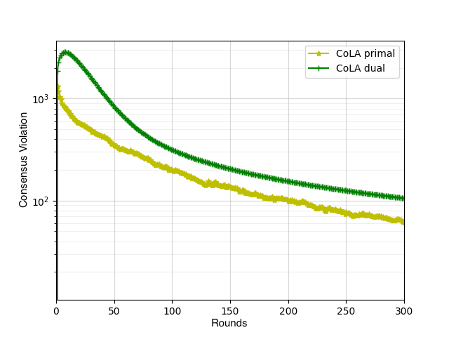
Figure 5: The consensus violation curve of CoLa in Figure 2.
 

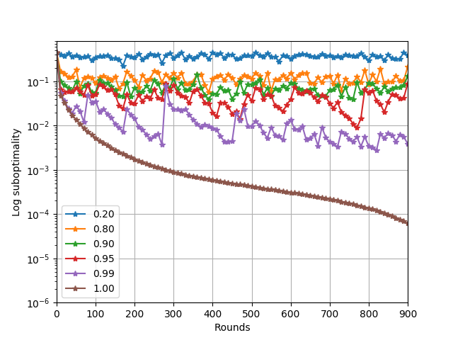
Figure 6: Same settings as Figure 4 except that $\mathbf{x}_{[k]}$ are reset after node $k$ leaving the network.
 

Appendix E Details regarding extensions

E.1 Fault tolerance and time varying graphs

In this section we extend framework CoLa to handle fault tolerance and time varying graphs. Here we assume when a node leave the network, their local variables $\mathbf{x}$ are frozen. We use same assumptions about the fault tolerance model in (Smith et al., 2017).

Definition 5 (Per-Node-Per-Iteration-Approximation Parameter).

At each iteration $t$, we define the accuracy level of the solution calculated by node $k$ to its subproblem as

$$\theta_{k}^{t}:=\frac{\mathscr{G}^{\sigma^{\prime}}_{k}(\Delta{\bf x}^{(t)}_{k};{\bf x}_{[k]}^{(t)},\mathbf{v}_{k}^{(t)})-\mathscr{G}^{\sigma^{\prime}}_{k}({\Delta{\bf x}}^{\star}_{k};{\bf x}_{[k]}^{(t)},\mathbf{v}_{k}^{(t)})}{\mathscr{G}^{\sigma^{\prime}}_{k}({\bf 0};{\bf x}_{[k]}^{(t)},\mathbf{v}_{k}^{(t)})-\mathscr{G}^{\sigma^{\prime}}_{k}({\Delta{\bf x}}^{\star}_{k};{\bf x}_{[k]}^{(t)},\mathbf{v}_{k}^{(t)})}$$ (77)

where ${\Delta{\bf x}}^{\star}_{k}$ is the minimizer of the subproblem $\mathscr{G}^{\sigma^{\prime}}_{k}(\cdot;{\bf x}_{[k]}^{(t)},\mathbf{v}_{k}^{(t)})$. We allow this value to vary between [0, 1] with $\theta_{k}^{t}:=1$ meaning that no updates to subproblem $\mathscr{G}^{\sigma^{\prime}}_{k}$ are made by node $k$ at iteration $t$.

The flexible choice of $\theta_{k}^{t}$ allows the consideration of stragglers and fault tolerance. We also need the following assumption on $\theta_{k}^{t}$.

Assumption 2 (Fault Tolerance Model).

Let $\{\mathbf{x}^{(t)}\}_{t=0}^{T}$ be the history of iterates until the beginning of iteration $T$. For all nodes $k$ and all iterations $t$, we assume $p_{k}^{t}:={\cal{P}}[\theta_{k}^{t}=1]\leq p_{\text{max}}<1$ and $\hat{\Theta}_{k}^{T}:={\mathbb{E}}[\theta_{k}^{T}|\{\mathbf{x}^{(t)}\}_{t=0}^{T},\theta_{k}^{T}<1]\leq\Theta_{\text{max}}<1$.

In addition we write $\bar{\Theta}:=p_{\text{max}}+(1-p_{\text{max}})\Theta_{\text{max}}<1$. Another assumption on time varying model is necessary in order to maintain the same linear and sublinear convergence rate. It is from (Nedic et al., 2017, Assumption 1):

Assumption 3 (Time Varying Model).

Assume the mixing matrix $\mathcal{W}(t)$ is a function of time $t$. There exist a positive integer $B$ such that the spectral gap satisfies the following condition

$$\textstyle\sigma_{\text{max}}\left\{\prod_{i=t}^{t+B-1}\mathcal{W}(i)-\frac{1}{K}\mathbf{1}\mathbf{1}^{\top}\right\}\leq\beta_{\text{max}}\qquad\forall~{}t\geq 0.$$

We change the Algorithm 1 such that it performs gossip step for $B$ times between solving subproblems. In this way, the convergence rate on time varying mixing matrix is similar to a static graph with mixing matrix $\prod_{i=t}^{t+B-1}\mathcal{W}(i)$. The sublinear/linear rate can be proved similarly.

E.2 Data dependent aggregation parameter

Definition 6 (Data-dependent aggregation parameter).

In Algorithm 1, the aggregation parameter $\gamma$ controls the level of adding $\gamma$ versus averaging $\gamma:=\frac{1}{K}$ of the partial solution from all machines. For the convergence discussed below to hold, the subproblem parameter $\sigma^{\prime}$ must be chosen not smaller than

$$\sigma^{\prime}\geq\sigma^{\prime}_{\text{min}}:=\gamma\max_{{\bf x}\in{\mathbb{R}}^{n}}\frac{\left\lVert{\mathbf{A}{\bf x}}\right\rVert^{2}}{\sum_{k=1}^{K}\left\lVert{\mathbf{A}{\bf x}_{[k]}}\right\rVert^{2}}$$ (78)

The simple choice of $\sigma^{\prime}:=\gamma K$ is valid for (78), closer to the actual bound given in $\sigma^{\prime}_{\text{min}}$.

E.3 Hessian subproblem

If the Hessian matrix of $f$ is available, it can be used to define better local subproblems, as done in the classical distributed setting by (Gargiani, 2017; Lee and Chang, 2017; Dünner et al., 2018; Lee et al., 2018). We use same idea in the decentralized setting, defining the improved subproblem

$$\begin{split}\mathscr{G}^{\sigma^{\prime}}_{k}(\Delta{\bf x};{\bf x}_{[k]},\mathbf{v}_{k}):=&\textstyle\frac{1}{K}f({\bf v}_{k})+\left\langle\sum_{l=1}^{K}\mathcal{W}_{kl}\nabla f({\bf v}_{l}),\mathbf{A}\Delta{\bf x}_{[k]}\right\rangle\\ &\textstyle+\frac{1}{2}(\mathbf{A}\Delta{\bf x}_{[k]})^{\top}\left(\sum_{l=1}^{K}\mathcal{W}_{kl}\nabla^{2}f({\bf v}_{l})\right)\mathbf{A}\Delta{\bf x}_{[k]}+\sum_{i\in\mathcal{P}_{k}}g_{i}(x_{i}+{\Delta x_{i}})\end{split}$$ (79)

The sum of previous subproblems satisfies the following relations

$$\sum_{k=1}^{K}\mathscr{G}^{\sigma^{\prime}}_{k}({\bf 0};{\bf x}^{(t+1)}_{[k]},\mathbf{v}_{k}^{(t+1)})$$

$$= \frac{1}{K}\sum_{k=1}^{K}f\left(\sum_{l=1}^{K}\mathcal{W}_{kl}{\bf v}_{l}^{(t)}+\gamma K\mathbf{A}\Delta{\bf x}_{[k]}\right)+\sum_{i\in\mathcal{P}_{k}}g_{i}(x_{i}^{(t)}+(\Delta{\bf x}_{[k]})_{i})$$

$$\leq \frac{1}{K}\sum_{k=1}^{K}\sum_{l=1}^{K}\mathcal{W}_{kl}\left\{f({\bf v}_{l}^{(t)})+\langle\nabla f({\bf v}_{l}^{(t)}),\gamma K\mathbf{A}\Delta{\bf x}_{[k]}\rangle+\frac{1}{2}(\mathbf{A}\Delta{\bf x}_{[k]})^{\top}\nabla^{2}f({\bf v}_{l}^{(t)})\mathbf{A}\Delta{\bf x}_{[k]}\right\}$$

$$+\sum_{i\in\mathcal{P}_{k}}g_{i}(x_{i}^{(t)}+(\Delta{\bf x}_{[k]})_{i})$$

$$= \sum_{k=1}^{K}\mathscr{G}^{\sigma^{\prime}}_{k}(\Delta{\bf x};{\bf x}_{[k]}^{(t)},\mathbf{v}_{k}^{(t)})\leq\sum_{k=1}^{K}\mathscr{G}^{\sigma^{\prime}}_{k}({\bf 0};{\bf x}_{[k]}^{(t)},\mathbf{v}_{k}^{(t)})$$

This means that the sequence $\big{\{}\sum_{k=1}^{K}\mathscr{G}^{\sigma^{\prime}}_{k}({\bf 0};{\bf x}_{[k]}^{(t)},\mathbf{v}_{k}^{(t)})\big{\}}_{t=0}^{\infty}$ is monotonically non-increasing. Following the reasoning in this paper, we can have similar convergence guarantees for both strongly convex and general convex problems. Formalizing all detailed implications here would be out of the scope of this paper, but the main point is that the second-order techniques developed for the CoCoA framework also have their analogon in the decentralized setting.

References

- Tsitsiklis et al. [1986] John N Tsitsiklis, Dimitri P Bertsekas, and Michael Athans. Distributed asynchronous deterministic and stochastic gradient optimization algorithms. IEEE Transactions on Automatic Control, 31(9):803–812, 1986.
- Nedic and Ozdaglar [2009] Angelia Nedic and Asuman Ozdaglar. Distributed subgradient methods for multi-agent optimization. IEEE Transactions on Automatic Control, 54(1):48–61, 2009.
- Duchi et al. [2012] J C Duchi, A Agarwal, and M J Wainwright. Dual Averaging for Distributed Optimization: Convergence Analysis and Network Scaling. IEEE Transactions on Automatic Control, 57(3):592–606, March 2012.
- Shi et al. [2015] Wei Shi, Qing Ling, Gang Wu, and Wotao Yin. Extra: An exact first-order algorithm for decentralized consensus optimization. SIAM Journal on Optimization, 25(2):944–966, 2015.
- Mokhtari and Ribeiro [2016] Aryan Mokhtari and Alejandro Ribeiro. DSA: Decentralized double stochastic averaging gradient algorithm. Journal of Machine Learning Research, 17(61):1–35, 2016.
- Nedic et al. [2017] Angelia Nedic, Alex Olshevsky, and Wei Shi. Achieving geometric convergence for distributed optimization over time-varying graphs. SIAM Journal on Optimization, 27(4):2597–2633, 2017.
- Cevher et al. [2014] Volkan Cevher, Stephen Becker, and Mark Schmidt. Convex Optimization for Big Data: Scalable, randomized, and parallel algorithms for big data analytics. IEEE Signal Processing Magazine, 31(5):32–43, 2014.
- Smith et al. [2018] Virginia Smith, Simone Forte, Chenxin Ma, Martin Takác, Michael I Jordan, and Martin Jaggi. CoCoA: A General Framework for Communication-Efficient Distributed Optimization. Journal of Machine Learning Research, 18(230):1–49, 2018.
- Zhang et al. [2015] Sixin Zhang, Anna E Choromanska, and Yann LeCun. Deep learning with Elastic Averaging SGD. In NIPS 2015 - Advances in Neural Information Processing Systems 28, pages 685–693, 2015.
- Wang et al. [2017] Jialei Wang, Weiran Wang, and Nathan Srebro. Memory and Communication Efficient Distributed Stochastic Optimization with Minibatch Prox. In ICML 2017 - Proceedings of the 34th International Conference on Machine Learning, pages 1882–1919, June 2017.
- Dünner et al. [2016] Celestine Dünner, Simone Forte, Martin Takác, and Martin Jaggi. Primal-Dual Rates and Certificates. In ICML 2016 - Proceedings of the 33th International Conference on Machine Learning, pages 783–792, 2016.
- Jaggi et al. [2014] Martin Jaggi, Virginia Smith, Martin Takác, Jonathan Terhorst, Sanjay Krishnan, Thomas Hofmann, and Michael I Jordan. Communication-efficient distributed dual coordinate ascent. In Advances in Neural Information Processing Systems, pages 3068–3076, 2014.
- Scaman et al. [2017] Kevin Scaman, Francis R. Bach, Sébastien Bubeck, Yin Tat Lee, and Laurent Massoulié. Optimal algorithms for smooth and strongly convex distributed optimization in networks. In Proceedings of the 34th International Conference on Machine Learning, ICML 2017, Sydney, NSW, Australia, 6-11 August 2017, pages 3027–3036, 2017.
- Scaman et al. [2018] Kevin Scaman, Francis Bach, Sébastien Bubeck, Yin Tat Lee, and Laurent Massoulié. Optimal algorithms for non-smooth distributed optimization in networks. arXiv preprint arXiv:1806.00291, 2018.
- Jakovetic et al. [2012] Dusan Jakovetic, Joao Xavier, and Jose MF Moura. Convergence rate analysis of distributed gradient methods for smooth optimization. In Telecommunications Forum (TELFOR), 2012 20th, pages 867–870. IEEE, 2012.
- Yuan et al. [2016] Kun Yuan, Qing Ling, and Wotao Yin. On the convergence of decentralized gradient descent. SIAM Journal on Optimization, 26(3):1835–1854, 2016.
- Shi et al. [2014] Wei Shi, Qing Ling, Kun Yuan, Gang Wu, and Wotao Yin. On the Linear Convergence of the ADMM in Decentralized Consensus Optimization. IEEE Transactions on Signal Processing, 62(7):1750–1761, 2014.
- Wei and Ozdaglar [2013] Ermin Wei and Asuman Ozdaglar. On the O(1/k) Convergence of Asynchronous Distributed Alternating Direction Method of Multipliers. arXiv, July 2013.
- Bianchi et al. [2016] Pascal Bianchi, Walid Hachem, and Franck Iutzeler. A coordinate descent primal-dual algorithm and application to distributed asynchronous optimization. IEEE Transactions on Automatic Control, 61(10):2947–2957, 2016.
- Lian et al. [2017] Xiangru Lian, Ce Zhang, Huan Zhang, Cho-Jui Hsieh, Wei Zhang, and Ji Liu. Can decentralized algorithms outperform centralized algorithms? a case study for decentralized parallel stochastic gradient descent. In Advances in Neural Information Processing Systems, pages 5336–5346, 2017.
- Lian et al. [2018] Xiangru Lian, Wei Zhang, Ce Zhang, and Ji Liu. Asynchronous decentralized parallel stochastic gradient descent. In ICML 2018 - Proceedings of the 35th International Conference on Machine Learning, 2018.
- Tang et al. [2018a] Hanlin Tang, Xiangru Lian, Ming Yan, Ce Zhang, and Ji Liu. D2: Decentralized training over decentralized data. arXiv preprint arXiv:1803.07068, 2018a.
- Tang et al. [2018b] Hanlin Tang, Shaoduo Gan, Ce Zhang, Tong Zhang, and Ji Liu. Communication compression for decentralized training. In NIPS 2018 - Advances in Neural Information Processing Systems, 2018b.
- Wu et al. [2018] Tianyu Wu, Kun Yuan, Qing Ling, Wotao Yin, and Ali H Sayed. Decentralized consensus optimization with asynchrony and delays. IEEE Transactions on Signal and Information Processing over Networks, 4(2):293–307, 2018.
- Sirb and Ye [2018] Benjamin Sirb and Xiaojing Ye. Decentralized consensus algorithm with delayed and stochastic gradients. SIAM Journal on Optimization, 28(2):1232–1254, 2018.
- Yang [2013] Tianbao Yang. Trading Computation for Communication: Distributed Stochastic Dual Coordinate Ascent. In NIPS 2014 - Advances in Neural Information Processing Systems 27, 2013.
- Ma et al. [2015] Chenxin Ma, Virginia Smith, Martin Jaggi, Michael I Jordan, Peter Richtárik, and Martin Takác. Adding vs. Averaging in Distributed Primal-Dual Optimization. In ICML 2015 - Proceedings of the 32th International Conference on Machine Learning, pages 1973–1982, 2015.
- Dünner et al. [2018] Celestine Dünner, Aurelien Lucchi, Matilde Gargiani, An Bian, Thomas Hofmann, and Martin Jaggi. A Distributed Second-Order Algorithm You Can Trust. In ICML 2018 - Proceedings of the 35th International Conference on Machine Learning, pages 1357–1365, July 2018.
- Agarwal and Duchi [2011] Alekh Agarwal and John C Duchi. Distributed delayed stochastic optimization. In Advances in Neural Information Processing Systems, pages 873–881, 2011.
- Zinkevich et al. [2010] Martin Zinkevich, Markus Weimer, Lihong Li, and Alex J Smola. Parallelized stochastic gradient descent. In Advances in Neural Information Processing Systems, pages 2595–2603, 2010.
- Zhang and Lin [2015] Yuchen Zhang and Xiao Lin. Disco: Distributed optimization for self-concordant empirical loss. In International conference on machine learning, pages 362–370, 2015.
- Reddi et al. [2016] Sashank J Reddi, Jakub Konecnỳ, Peter Richtárik, Barnabás Póczós, and Alex Smola. Aide: Fast and communication efficient distributed optimization. arXiv preprint arXiv:1608.06879, 2016.
- Gargiani [2017] Matilde Gargiani. Hessian-CoCoA: a general parallel and distributed framework for non-strongly convex regularizers. Master’s thesis, ETH Zurich, June 2017.
- Lee and Chang [2017] Ching-pei Lee and Kai-Wei Chang. Distributed block-diagonal approximation methods for regularized empirical risk minimization. arXiv preprint arXiv:1709.03043, 2017.
- Lee et al. [2018] Ching-pei Lee, Cong Han Lim, and Stephen J Wright. A distributed quasi-newton algorithm for empirical risk minimization with nonsmooth regularization. In ACM International Conference on Knowledge Discovery and Data Mining, 2018.
- Smith et al. [2017] Virginia Smith, Chao-Kai Chiang, Maziar Sanjabi, and Ameet Talwalkar. Federated Multi-Task Learning. In NIPS 2017 - Advances in Neural Information Processing Systems 30, 2017.
- Konecnỳ et al. [2015] Jakub Konecnỳ, Brendan McMahan, and Daniel Ramage. Federated optimization: Distributed optimization beyond the datacenter. arXiv preprint arXiv:1511.03575, 2015.
- Konecnỳ et al. [2016] Jakub Konecnỳ, H Brendan McMahan, Felix X Yu, Peter Richtarik, Ananda Theertha Suresh, and Dave Bacon. Federated learning: Strategies for improving communication efficiency. arXiv preprint arXiv:1610.05492, 2016.
- McMahan et al. [2017] Brendan McMahan, Eider Moore, Daniel Ramage, Seth Hampson, and Blaise Aguera y Arcas. Communication-efficient learning of deep networks from decentralized data. In Artificial Intelligence and Statistics, pages 1273–1282, 2017.
- Boyd et al. [2011] Stephen Boyd, Neal Parikh, Eric Chu, Borja Peleato, Jonathan Eckstein, et al. Distributed optimization and statistical learning via the alternating direction method of multipliers. Foundations and Trends® in Machine learning, 3(1):1–122, 2011.
- Stich et al. [2018] Sebastian U. Stich, Jean-Baptiste Cordonnier, and Martin Jaggi. Sparsified sgd with memory. In NIPS 2018 - Advances in Neural Information Processing Systems, 2018.
- Rockafellar [2015] Ralph Tyrell Rockafellar. Convex analysis. Princeton university press, 2015.
- Hastings [1970] W Keith Hastings. Monte carlo sampling methods using markov chains and their applications. Biometrika, 57(1):97–109, 1970.
- Paszke et al. [2017] Adam Paszke, Sam Gross, Soumith Chintala, Gregory Chanan, Edward Yang, Zachary DeVito, Zeming Lin, Alban Desmaison, Luca Antiga, and Adam Lerer. Automatic differentiation in pytorch. In NIPS Workshop on Autodiff, 2017.
- Pedregosa et al. [2011] F. Pedregosa, G. Varoquaux, A. Gramfort, V. Michel, B. Thirion, O. Grisel, M. Blondel, P. Prettenhofer, R. Weiss, V. Dubourg, J. Vanderplas, A. Passos, D. Cournapeau, M. Brucher, M. Perrot, and E. Duchesnay. Scikit-learn: Machine learning in Python. Journal of Machine Learning Research, 12:2825–2830, 2011.