pnasresearcharticle \leadauthorHaller \significancestatement Observations of tracer transport in fluids generally reveal highly complex patterns shaped by an intricate network of transport barriers and enhancers. The elements of this network appear to be universal for small diffusivities, independent of the tracer and its initial distribution. Here, we develop a mathematical theory for weakly diffusive tracers to predict transport barriers and enhancers solely from the flow velocity, without reliance on diffusive or stochastic simulations. Our results yield a simplified computational scheme for diffusive transport problems, such as the estimation of salinity redistribution for climate studies and the forecasting of oil spill spreads on the ocean surface. \authorcontributionsG.H. and D.K. designed the research. G.H. developed the theory and wrote the manuscript with contributions from the other authors. D.K. developed the computational algorithm and carried out the numerical simulations. F.K. proved the asymptotic expansion formula for the transport functional. \authordeclarationThe authors declare no conflict of interest. \correspondingauthor2To whom correspondence should be addressed. E-mail: georgehaller@ethz.ch
Material Barriers to Diffusive and Stochastic Transport
Abstract
We seek transport barriers and transport enhancers as material surfaces across which the transport of diffusive tracers is minimal or maximal in a general, unsteady flow. We find that such surfaces are extremizers of a universal, non-dimensional transport functional whose leading-order term in the diffusivity can be computed directly from the flow velocity. The most observable (uniform) transport extremizers are explicitly computable as null-surfaces of an objective transport tensor. Even in the limit of vanishing diffusivity, these surfaces differ from all previously identified coherent structures for purely advective fluid transport. Our results extend directly to stochastic velocity fields and hence enable transport barrier and enhancer detection under uncertainties.
keywords:
diffusive transport coherent structures turbulence variational calculus-2pt
1 Introduction
Transport barriers, i.e., observed inhibitors of the spread of substances in flows, provide a simplified global template to analyze mixing without testing various initial concentrations and tracking their pointwise evolution in detail. Even though such barriers are well documented in several physical disciplines, including geophysical flows (1), fluid dynamics (2), plasma fusion (3), reactive flows (4) and molecular dynamics (5), no generally applicable theory for their defining properties and detection has emerged. In this paper, we seek to fill this gap by proposing a mathematical theory of transport barriers and enhancers from first principles in the physically ubiquitous regime of small diffusivities (high Péclet numbers).
Diffusive transport is governed by a time-dependent partial differential equation (PDE), whose numerical solution requires knowledge of the initial concentration, the exact diffusivity and the boundary conditions. Persistently high gradients make this transport PDE challenging to solve accurately for weakly diffusive processes, such as temperature and salinity transport in the ocean and vorticity transport in high-Reynolds-number turbulence. That is why one often neglects diffusion and focuses on the purely advective redistribution of the substance, governed by an ordinary differential equation that only involves a deterministic flow velocity field. In that purely advective setting, a transport barrier is often described as a surface with zero material flux. While plausible at first sight, this view actually renders transport barriers grossly ill-defined. Indeed, any codimension-one surface of carrier fluid trajectories (material surface) experiences zero material flux, and hence is a barrier by this definition (Fig. 1).
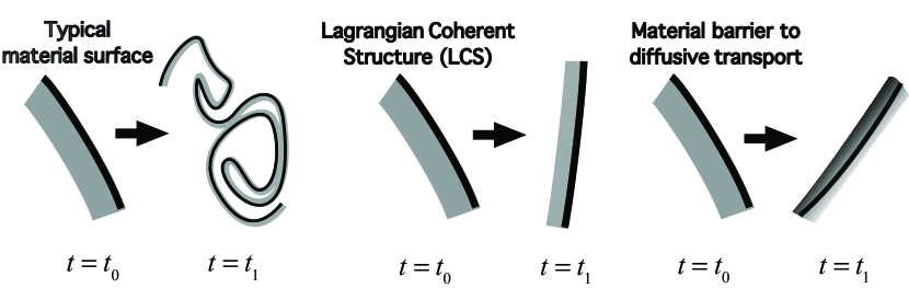
This ambiguity has ignited interest in Lagrangian coherent structures (LCSs, see Fig. 1), which are material surfaces that do not simply block but also organize conservative tracers into coherent patterns (6, 7, 8, 9). Due to differing views on finite-time material coherence, however, each available approach yields (mildly or vastly) different structures as LCSs (10). These discrepancies suggest that even purely advective coherent structure detection would benefit from being viewed as the zero-diffusion limit of diffusive barrier detection. Indeed, transport via diffusion through a material surface is a uniquely defined, fundamental physical quantity, whose extremum surfaces can be defined without invoking any special notion of coherence.
A large number of prior approaches to weakly diffusive transport exist, only some of which will be possible to mention here. Among these, spatially localized expansions around simple advective solutions provide appealingly detailed temporal predictions for simple velocity fields (11, 12, 13). Writing the advection-diffusion equation in Lagrangian coordinates suggests a quasi-reduction to a one-dimensional diffusion PDE along the most contracting direction, yielding asymptotic scaling laws for stretching and folding statistics along chaotic trajectories (14, 15). Observed transport barriers, however, are not chaotic, and the formal asymptotic expansions used in these subtle arguments remain unjustified. As alternatives, the effective diffusivity approach of (16) and the residual velocity field concept (17) offer attractive visualization tools for regions of enhanced or suppressed transport. Both approaches, however, target already performed diffusive simulations, and hence provide descriptive diagnostics rather than prediction tools.
Here we address the diffusive tracer transport problem in its purest, original form. Namely, we seek transport barriers as space-dividing (codimension-one) material surfaces that inhibit diffusive transport more than neighboring surfaces do. Locating material diffusion barriers without simulating diffusion and without reliance on specific initial concentration distributions is the physical problem we define and solve here in precise mathematical terms, assuming only incompressibility and small diffusion. In the limit of vanishing diffusion, our approach also provides a unique, physical definition of LCSs as material surfaces that will block transport most efficiently under the addition of the slightest diffusion or uncertainty to an idealized, purely advective mixing problem. Since the notion of transport through a surface is quantitative and universally accepted, this definition of an LCS eliminates the current ambiguity in advective mixing studies, with different approaches identifying different structures as coherent (10).
2 Transport tensor and transport functional
The advection-diffusion equation for a tracer is given by (18)
| (1) |
where denotes the gradient operation with respect to the spatial variable on a compact domain with ; is an -dimensional, incompressible, smooth velocity field generating the advective transport of whose initial distribution is ; is the dimensionless, positive definite diffusion-structure tensor describing possible anisotropy and temporal variation in the diffusive transport of ; is a small diffusivity parameter rendering the full diffusion tensor small in norm. We assume that the initial concentration is of class , and the diffusion tensor is at least Hölder-continuous, which certainly holds if it is continuously differentiable.
The Lagrangian flow map induced by is , mapping initial material element positions to their later positions at time . We assume that trajectories stay in the domain of known velocities, i.e., holds for all times of interest. We will denote by the gradient of with respect to initial positions .
Let be a time-evolving, -dimensional material surface in with boundary and with initial position . By construction, the advective flux of through vanishes and hence only the diffusive part of the flux vector on the right-hand side of (1) generates transport through . The total transport of through over a time interval is therefore given by
| (2) |
with denoting the area element on and denoting the unit normal to at a point . Let and denote the area element and oriented unit normal vector field on the initial surface . Then, by the classic surface element deformation formula (19), and by the chain rule applied to , we can rewrite the total transport (2) through as
| (3) |
with the tensor defined as
| (4) |
We note that by incompressibility, and that
| (5) |
holds in case of isotropic diffusion (), with denoting the Cauchy–Green strain tensor (19).
As we show in SI Appendix S1, under our assumptions on and , (3) can be equivalently re-written as
| (6) |
with the symbol referring to a quantity that, even after division by , tends to zero as . Proving (6) is subtle, because (1) is a singularly perturbed PDE for small , and hence its solutions generally cannot be Taylor-expanded at , unless is integrable (20).
To systematically test the ability of the material surface to hinder the transport of over the time interval , we initialize the concentration field at time locally near so that is a level surface of along which has a constant magnitude . This universal choice of subjects each surface to the same, most diffusion-prone scalar configuration, ensuring equal detectability for all barriers in our analysis, independent of any specific initial concentration distribution. We can then write , and hence the total transport in (6) becomes
Here we have introduced the symmetric, positive definite transport tensor as the time-average of over The same averaged tensor was already proposed heuristically in (11) to simplify the Lagrangian version of (1).111 This heuristic simplification generally gives incorrect results for unsteady flows and can only be partially justified for steady flows (12). In our present context, however, arises without any heuristics.
Finally, to give a dimensionless characterization of the transport through the surface over the period , we normalize by the diffusivity , by the transport time , by the initial concentration gradient magnitude , and by the surface area (or length, for ) of . This leads to the normalized total transport
| (7) |
for some , where the non-dimensional transport functional
| (8) |
is a universal measure of the leading-order diffusive transport through the material surface over the period . This functional enables a systematic comparison of the quality of transport through different material surfaces. Remarkably, can be computed for any initial surface directly from the trajectories of , without solving the PDE (1). Furthermore, as we show in SI Appendix S2, and hence are objective (frame-indifferent).
3 General equation for diffusive transport extremizers
By formula (7) and by the implicit function theorem, nondegenerate extrema of the normalized total transport are -close to those of the transport functional , for some . Initial positions of such transport-extremizing material surfaces are, therefore, necessarily solutions of the variational problem
| (9) |
with boundary conditions yet to be specified, given that the location and geometry of diffusive transport extremizers is unknown at this point. We will refer to minimizers of as diffusive transport barriers and to maximizers of as diffusive transport enhancers.
Carrying out the variational differentiation in (9) gives the equivalent extremum problem (cf. (21))
| (10) |
where is constant. To transform this problem to a form amenable to classical variational calculus, we need to reformulate (10) in terms of a (yet unknown) general parameterization of , and then express the integrand in terms of tangent vectors computed from this parametrization. As we show in SI Appendix S3, if , denotes the entry of the Gramian matrix of the parametrization, then after re-parametrization and passage from normal to tangent vectors in the integrand, we can rewrite the functional in (10) in the form
| (11) |
with the Lagrangian
| (12) |
The Euler–Lagrange equations associated with the Lagrangian (12) are given by the -dimensional set of coupled nonlinear, second-order PDEs
| (13) |
4 Uniform extremizers of diffusive transport
(13) has infinitely many solutions through any point of the physical space, yet most of these solution surfaces remain unobserved as significant barriers due to large variations in the concentration gradient along them. Most observable are transport extremizers that maintain a nearly uniform drop in the scalar concentration along them, implying that the transport-density along them is as uniform as possible.
As we show in SI Appendix S4, even perfectly uniform extremizers of exist and form the zero level set in the phase space of (13). As we see from (12), these uniform transport extremizer solutions of (13) satisfy the first-order family of PDEs
| (14) |
for any choice of the parameter . Note that, by construction, then equals to the uniform diffusive transport density across any subset of the material surface over the time interval .
An equivalent form of (14) follows from the observation that the functional is invariant under reparametrizations and hence can also be computed from the original, surface-normal-based form (10) of the underlying variational principle. The latter form simply gives on , which we further rewrite as
| (15) |
This reveals that diffusive transport extremizers are null-surfaces of the metric tensor , i.e., their normals have zero length in the metric defined by .
For such null-surfaces to exist through a point the metric generated by must have null directions. This limits the domain of existence of transport extremizers with uniform transport density to spatial domains where the eigenvalues of the positive definite tensor satisfy .
Finding computable sufficient conditions for the solutions of the variational problem in (10) to be minimizers does not appear to be within reach. Effective necessary conditions, however, can help greatly in identifying null surfaces of that are likely candidates for extremizers. One such necessary condition requires the trace of the tensor to be nonnegative, as we show in SI Appendix S5. This enables us to summarize our main results for transport extremizers in the following theorem.
Theorem 1
A uniform minimizer of the transport functional is necessarily a non-negatively traced null-surface of the tensor field , i.e,
| (16) |
holds at every point with unit normal to . Similarly, a uniform maximizer of is necessarily a non-positively traced null surface of the tensor field , i.e,
| (17) |
holds at every point .
Remark 1
Assume that the flow is two-dimensional ( and the diffusion is homogeneous and isotropic (. Then, replacing the averaged transport tensor with its unaveraged counterpart in our arguments, we obtain that closed material curves that extremize the diffusive flux uniformly at coincide with two-dimensional elliptic Lagrangian coherent structures LCSs (22). Similarly, replacing with the transport-rate tensor ,222Note that where is the classic rate-of-strain tensor for the velocity field we obtain that closed curves that uniformly extremize the diffusive flux-rate at coincide with elliptic objective Eulerian coherent structures (OECSs) (23).
Remark 1 connects instantaneous flux and flux-rate extremizing surfaces under isotropic diffusion to LCSs and EOCSs. In the limit, however, material diffusion barriers identified by Theorem 1 differ from advective coherent structures identified in previous studies (cf. SI Appendix S7). While this conclusion is at odds with the usual assumptions of purely advective transport studies, it is mathematically consistent with the singular perturbation nature of the diffusion term in (1).
Remark 2
As seen in the proof of Theorem 1 in SI Appendix S5, measures how strongly the normalized transport changes from under localized normal perturbations at to a transport extremizer . Consequently, the Diffusion Barrier Strength (DBS), defined as
| (18) |
serves as an objective diagnostic scalar field that highlights centerpieces of regions filled with the most influential transport extremizers. Specifically, the time positions of the most prevailing diffusion barriers should be marked approximately by ridges of field, while the time positions of the least prevailing diffusion barriers should be close to trenches of . A similar conclusion holds for diffusion enhancers based on features of the field computed in backward time.
By Remark 2, features of the scalar field play a role analogous to that of the finite-time Lyapunov exponents (FTLEs) in purely advective transport (7). Unlike the FTLE field, however, is a predictive diagnostic (i.e., requires no diffusive simulation) and arises directly from the technical construction of diffusion extremizers (rather than being one possible indicator of their anticipated properties). Still, is a visual diagnostic, while Theorem 1 provides the exact equations that diffusion barriers and enhancers satisfy.
5 Application to two-dimensional flows
Here we solve the general barrier-enhancer equations (16)-(17) explicitly for two-dimensional flows and write out a more specific form of the diagnostic for such flows. In two dimensions (, a one-dimensional transport extremizer curve is parametrized by a single scalar parameter . As we show in SI Appendix S6, the Lagrangian in (12) then simplifies to
| (19) |
with the tensor field
| (20) |
denoting the time-averaged, diffusivity-structure-weighted version of the classic right Cauchy–Green strain tensor introduced in (5). The Euler–Lagrange (13) now forms a four-dimensional system of ODEs, which we write out for reference in SI Appendix S6. Uniform transport barriers and enhancers lie in the set in the phase space of this ODE. Equating (19) with zero, we obtain that solutions in satisfy , and hence are precisely the null-geodesics of the one-parameter-family of tensors
| (21) |
which are Lorentzian (i.e., indefinite) metric tensors on the spatial domain satisfying . This extends the mathematical analogy pointed out in (22, 24) between coherent vortex boundaries and photon spheres around black holes from advective to diffusive mixing. In this analogy, the role of the relativistic metric tensor on the four-dimensional space-time is replaced by the tensor on the two-dimensional physical space of initial conditions.
We seek unit tangent vectors to null-geodesics of as a linear combination of the unit eigenvectors corresponding to the eigenvalues of the positive definite tensor . Substituting this linear combination into and solving for gives the direction field family
| (22) |
for null-geodesics of , defined only on the domain where Trajectories of experience uniform pointwise transport density over the time interval For homogeneous, isotropic diffusion (), we have by incompressibility (cf. SI Appendix S6). Consequently, the scalar diagnostic featured in Remark 2 takes the specific form . Finally, as we show in SI Appendix S6, there are only three types of robust barriers to diffusion in two-dimensional flows: fronts, jet cores and families of closed material curves forming material vortices. This is consistent with observations of large-scale geophysical flows (1).
6 Particle transport extremizers in stochastic velocity fields
Here, we show how our results on barriers to diffusive scalar transport carry over to probabilistic transport barriers to fluid particle motion with uncertainties. Such motions are typically modeled by diffusive Itô processes of the form
| (23) |
where is the random position vector of a particle at time ; denotes the incompressible, deterministic drift in the particle motion; and in an -dimensional Wiener process with diffusion matrix . Here the dimensionless, nonsingular diffusion structure matrix is with respect to the small parameter .
Let denote the probability density function (PDF) for the current particle position with initial condition . This PDF is known to satisfy the classic Fokker-Planck equation (25)
| (24) |
We can rewrite (24) as
| (25) |
which is of advection-diffusion-form, (1), if is incompressible, i.e., if
| (26) |
Assuming (26) (which holds, e.g., for homogeneous diffusion), we define the probabilistic transport tensor as the time-average of
We then conclude that all our results on diffusive scalar transport in a deterministic velocity field carry over automatically to particle transport in the stochastic velocity field (23) with the substitution . Namely, we have
Theorem 2
This result enables a purely deterministic computation of observed surfaces of particle accumulation and particle clearance without a Monte–Carlo simulation for (23).
7 Numerical implementation and example
For a two-dimensional velocity field and diffusion-structure tensor , the main algorithmic steps in locating diffusion barriers over a time interval are as follows (cf. SI Appendix S7 for more detail and a simple example):
- (A1)
-
Define a Lagrangian grid of initial conditions; generate trajectories of the velocity field with initial conditions at time .
- (A2)
- (A3)
-
Compute the diffusion-barrier-strength diagnostic . Its ridges and trenches highlight the most influential diffusion barriers (backward-time fronts and jet cores, respectively) at time .
- (A4)
-
Compute eigenvalues , and corresponding eigenvectors , of . Compute closed diffusion barriers as limit cycles of (22). Outermost members of the limit-cycle families mark diffusion-based material vortex boundaries at time .
- (A5)
-
To locate time- positions of material diffusion barriers, advect them using the flow map .
For probabilistic diffusion barriers in the stochastic velocity field (23), apply steps A1-A5 after setting .
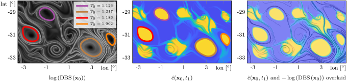
Our main example will illustrate steps (A1)-(A5) in the identification of boundaries for the largest mesoscale eddies in the Southern Ocean. Known as Agulhas rings, theses eddies are believed to contribute significantly to global circulation and climate via the warm and salty water they ought to carry (26). Several studies have sought to estimate material transport via these eddies by determining their boundaries from different material coherence principles, which all tend to give different results (22, 27, 28, 29, 30) Here, for the first time, we locate the boundaries of Agulhas rings based on the very principle that makes them significant: their role as universal barriers to the diffusion of relevant ocean water attributes they transport.
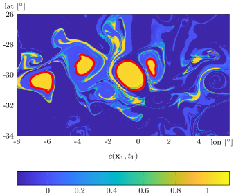
Figure 2 shows diffusive coherent Agulhas ring boundaries and surrounding diffusive barriers (backward-time fronts) in the Southern Ocean, computed via steps (A1)-(A5) from satellite-altimetry-based surface velocities (cf. SI Appendix S7 for more detail on the data set). The predicted material ring boundaries are obtained as described in step (A4). This prediction is confirmed by a diffusion simulation with Péclet number ; see also the Eulerian analogue in Fig. S4 of the diffused concentration in Supporting Animation SA1. Figure 2c also confirms a similar barrier role for the ridges of which closely align with observed open barriers to diffusive transport.
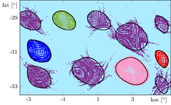
Figure 3 shows the final result of a Monte–Carlo simulation of (23) in the Lagrangian frame (cf. SI Appendix S7), given by
with homogeneous diffusion-structure matrix , whose Fokker–Planck equation coincides with the advection–diffusion equation in our previous simulation. The figure confirms the role of the ring boundaries (computed from the deterministic velocity field) as sharp barriers to particle transport under uncertainties in the velocity field. We show the evolving Monte–Carlo simulation in Supporting Animations SA2-SA3.
8 Conclusions
We have pointed out that the presence of the slightest diffusion in a deterministic flow yields an unambiguous, first-principles-based physical definition for transport barriers as material surfaces that block diffusive transport the most efficiently. We have found that in any dimension, such barriers lie close to minimizers of a universal, non-dimensionalized transport functional that measures the leading-order diffusive transport through material surfaces. Of these minimizers, a special set of most observable barriers is formed by those that maintain uniformly high concentration gradients, and hence uniform transport density, along themselves. Even such uniform barriers, however, will generally differ from coherent structures identified from purely advective considerations (Remark 1). Beyond the exact differential equations describing transport barriers, we have obtained a predictive diagnostic field, , that signals barrier location and strength from purely advective computations (Remark 2). Finally, we have discussed how the proposed methodology identifies probabilistic material barriers and enhancers to particle transport in multi-dimensional stochastic velocity fields.
Our results identify the main enhancers and inhibitors of transport in diffusive and random flows without costly numerical solutions of PDEs or Monte-Carlo simulations of stochastic flow models. By construction, the structures we obtain are robust with respect to small diffusive effects, including measurement uncertainties in observational velocity data or modeling errors in numerically generated velocity fields. Our detection scheme for transport extremizers is independent of the local availability of the diffusive tracer and of the initial distribution of its gradient field. The theoretically optimal transport extremizers identified here should also be useful as benchmarks for the development for future diagnostics targeting transport barriers in sparse data. Further theoretical work is required for a more detailed classification of diffusion extremizers in higher dimensions and in compressible flows. On the computational side, the accurate identification of diffusion extremizers identified here requires efficient numerical schemes for null-surfaces. On the applications side, further examples of practically relevant and multi-scale velocity fields need to be analyzed in detail to assess further practical implications of the barrier-detection method introduced here.
Acknowledgements
We are grateful to R Abernathey, FJ Beron–Vera, T Breunung, S Katsanoulis, A Constantin, M Mathur, G Pavliotis, M Rubin and J-L Thiffeault for useful discussions and comments, and to N Schilling for contributions to the animation code. GH and DK acknowledge support from the Turbulent Superstructures priority program of the German National Science Foundation (DFG).
S1: Expansion of the total transport in
We denote the restriction of the concentration field to trajectories of the velocity field by . We then use the advection-diffusion equation to conclude that the time-derivative of satisfies
| (27) |
Introducing the Lagrangian diffusion structure tensor , we can rewrite (27) as
| (28) |
A lengthy calculation leads to the Lagrangian form of the advection-diffusion equation as (11, 12, 14, 15)
| (29) |
Taking Lagrangian spatial gradient of both sides and integrating in time, we obtain
| (30) |
Substitution of (30) into the definition of then gives
We will now prove that the second term in this equation is of order , i.e.,
| (31) |
To this end, we need estimates on the solution of (29), which we rewrite here using the tensor as
| (32) | ||||
By our assumption of Hölder continuity for and smoothness for all other quantities involved, we obtain that is Hölder continuous. Specifically, for any entry of the matrix representation of , we have the bounds
| (33) |
for some constant and for all and . By the positive definiteness of , we also have
| (34) |
which implies the bounds
| (35) |
for all and . Next, we observe that (31) is satisfied when
| (36) |
holds for some , as one obtains using (30) and estimating the supremum norm in and using (33). Using the assumption that we will now show that (36) holds, and hence (31) is indeed satisfied. In our presentation, we will utilize a scaling approach described in (31).
Introducing the rescaled time variable as well as the shifted and rescaled concentration , then setting , we can rewrite (32) as
| (37) |
Condition (36) is then equivalent to
| (38) |
for some . Let
| (39) | ||||
for and , denote the fundamental solution of the homogeneous, second-order part of (37). For later computations, we note that with the -dimensional volume element , we have the estimate
| (40) |
where we have used the inequalities in (35). With the rescaled spatial variable and the rescaled volume form defined as
| (41) |
we define the set to obtain from (40) the estimate
| (42) |
where we have used that . We also recall from (31) (Theorem 3, p. 8), that for any continuous function , the integral
| (43) |
is continuously-differentiable with respect to and satisfies
| (44) |
As shown in (31) (Theorem 9, p.21), the variation of constants formula applied to (37) gives its solution in the form
| (45) |
for some (not explicitly known) function that satisfies the estimate
| (46) |
for any constant , where is the Hölder-exponent in (33).
To estimate the spatial gradient of , we use the formula for the -derivative of (45) in (44) to obtain
| (47) |
where we also used the definition (39) in evaluating . From (35), we obtain , and hence we can further write (47) as
| (48) |
Next, as in the calculation of the integral in (40), we use the scaling (41) in (48) to obtain
| (49) |
To estimate the spatial gradient of in (45), we proceed similarly by using the growth condition (46) to obtain
| (50) |
Since is bounded, there exists a ball of radius such that and therefore, noticing that by , we find that
| (51) |
As in (47), we can estimate the integral of to obtain
| (52) |
The estimates (49)-(52) together prove (38), which then implies (36), which in turn implies (31), as claimed.
S2: Objectivity of the transport tensor
Physically, the Eulerian flux density at a point at time through a surface element with unit normal must be independent of rotations and translations of observer. Consequently, under an observer change
| (53) |
we must have and hence
where we have defined the transformed diffusion tensor
| (54) |
and used the fact that the area element remains unchanged under rigid-body rotations and translations embodied by (53). Using (54) together with in the definition of gives
This then proves the frame-indifference of the transport tensor . as a tensor acting on, and mapping back to, the initial configuration, which is unaffected by the frame change.
S3: Reformulation of the transport functional
Under a general parametrization of , the integral in the functional can be rewritten as
| (55) |
where , , denotes the entry of the Gramian matrix of the parametrization, with providing the surface are element on .
To express the integrand of (55) fully in terms of tangent vectors , we first consider a general invertible linear operator and a unit vector selected to be normal to an dimensional hyperplane of linearly independent vectors . Recall that the -dimensional area of the parallelepiped spanned by these vectors is equal to
with the entries of the Gramian matrix defined as Similarly, under the action of the operator the image vectors span the area
Now, the volume of the -dimensional parallelepiped formed by the vectors, is
and hence the image of this parallelepiped under has the oriented volume
| (56) | ||||
| (57) |
With the unit normal to the image hyperplane we can also write
| (58) |
Therefore, a comparison of (56) and (58) gives
| (59) |
Back to the integral (55), we note that the symmetric tensor is positive definite, and hence its inverse admits a unique symmetric, positive definite square root tensor that can be written as . Then, selecting and in formula (59), we conclude that the integral in (55) can be re-written as
which proves the final formula we have given for with the Lagrangian , as claimed.
S4: First integral and existence of uniform barriers
The Lagrangian has no explicit dependence of the independent variable , and hence Noether’s theorem provides partial conservation laws (cf., (32), Chapter 4, Example 4.2) for the associated Euler–Lagrange equation in the form
| (60) |
with referring to the Kronecker delta. A direct calculation, however, gives and hence no nontrivial conserved quantity can be reconstructed from (60).
Instead, we apply an argument that extends the Maupertuis principle derived for ordinary differential equations in (33) to partial differential equations. We start by considering another variational problem associated with of the form
| (61) |
As has no explicit dependence on , Noether’s theorem again applies and yields partial conservation laws given by (60). In contrast to , however, is a positively homogeneous function of degree two, and hence, by Euler’s theorem (34), we obtain from (60) for that
and hence is a first integral for the set of Euler–Lagrange partial differential equations
| (62) |
(Here we have used the shorthand notation and .) Consequently,
| (63) |
holds on the solutions of (62). We will now observe a close relationship between the solutions of (62) and the solutions of the original variational problem.
To obtain this relationship, we first rewrite the left-hand side of the Euler–Lagrange equation
| (64) |
for by substituting , which gives
| (65) | |||
| (66) |
whenever . Therefore, a substitution of any solution solution of the Euler–Lagrange (62) into (65) gives
where we have used (62) and (63). Therefore, all solutions of (65) satisfying
| (67) |
are also solutions on the Euler–Lagrange (64). Furthermore, since is constant along these solutions, is also constant along .
Next, we assume that is a solution of the Euler–Lagrange (64) for . Rewriting this equation using the relation , we obtain
| (68) |
We now introduce a solution-dependent rescaling of the parameter vector by defining the new independent variable vector as
so that, in the new variable , (68) becomes
where we have used the linearity of in . Therefore, any solution of (64) satisfying (67), and hence satisfying , is also a solution of (62) and thus conserves , and hence , as first integrals. Consequently, all solutions of (64) and (62) are equivalent as long as holds on them. This implies that the set , if nonempty, is an invariant set for the Euler–Lagrange equation of .
S5: Local necessary conditions for extrema
If is a stationary surface for a quotient functional with , then we have
with and . Consequently, local maxima (or minima) of coincide with the local maxima (or minima, respectively) of .
A simple necessary condition for a null-surface to be an extremizer of can be obtained by considering a small, surface-area-preserving perturbation to , where is a uniformly bounded, smooth function with , that is supported only in an neighborhood of the origin. The function then gives the parametrization of a perturbed hypersurface . Within the support of , the unit normal of the perturbed surface at must therefore satisfy
for some For values outside the support of , we have . One then obtains
where we have used that holds along , and that the support of has volume of order in . Therefore, if is a local minimizer of the functional , then we must necessarily have
Since the point along and the exact shape of (and hence have been arbitrary, this last inequality implies
| (69) |
Therefore, the tensor must be positive semidefinite on the tangent bundle of its null surface , if this null surface is a transport barrier.
Next, we derive a condition equivalent to (69) that is nevertheless easier to verify directly from the eigenvalues of . To this end, let us denote the eigenvalues of by
with denoting the eigenvalues of the positive definite tensor , as earlier. We observe that condition (69) implies Indeed, if or were satisfied, then would be definite and hence could have no nonempty null-surface .
We next show that
| (70) |
must necessarily hold. Indeed, assuming the opposite would imply, by the ordering of the eigenvalues, that holds, and hence would have two negative eigenvalues, and This would then necessarily imply that (otherwise the unit normal would necessarily have to be orthogonal to the eigenvectors of these two negative eigenvalues, and would necessarily take negative values in ). Therefore, (70) must be satisfied.
Finally, we show that
| (71) |
must hold. Indeed, assuming necessarily implies must hold, and hence, by (70), the local unit normal of , with coordinates with respect to the orthonormal eigenbasis of , must satisfy the equation
| (72) |
where all coefficients on the right-hand side are nonnegative, and at least is strictly positive. The surface defined by (72) is a codimension-one elliptical cone when the coefficients are nonzero, or the product of a lower-dimensional elliptical cone with a plane when some of these coefficients are zero. Consider now a codimension-one plane containing the normal and the axis. The intersection then consists of two lines, one through and another line through the mirror image of with respect to the axis. If the angle of and is more than than then the plane normal to also intersects transversely, and hence will change its sign within the tangent plane Consequently, the minimal possible angle between and , over all choices of at a point , cannot exceed , otherwise cannot be a diffusive transport minimizer. This minimal angle arises when is contained in the subspace of the elliptical cone that runs closest to the axis, i..e, when are zero. In this case, , and hence the angle between and exceeds , given that we have assumed . We, therefore, conclude that (71) must hold.
S6: Transport extremizers in two dimensions
We first introduce the diffusion-weighted Cauchy–Green strain tensor Denoting by the co-factor matrix of , we observe that by incompressibility (), we have
| (73) |
We further note that in case of homogeneous-isotropic diffusion (), we have , and hence (73) gives
| (74) |
which further implies
| (75) |
where denote the eigenvalues of corresponding to the orthonormal eigenbasis and denote the normalized eigenvectors of .
Using (74), we obtain the Lagrangian for two-dimensional flows in the form
which, together with (73), gives
with the simplified notation , , and . From this, we obtain the Euler–Lagrange equations for in coordinate form as
| . | |||
Recall that the boundary term arising in the conversion of the weak form of Euler–Lagrange equation to its strong form must vanish, which gives, in two dimensions, the requirement
with denoting just a pair of discrete points. Evaluating this condition along uniform extremizers and noting the relations and at , we obtain
This inner product only vanishes in the following three cases:
- ()
-
Normal boundary perturbations (front-type surfaces; This is only possible at a boundary point if is an eigenvector of , i.e., holds for some with denoting the unit eigenvectors of the tensor . This condition holds at maximal open null-geodesics of , i.e., -lines ending at points where has precisely one zero eigenvalue.
- ()
-
Boundary perturbations along a two-dimensional subspace (jet-core-type surfaces; ). This is only possible at a boundary point if the symmetric tensor has two zero eigenvalues. That happens precisely when has two repeated eigenvalues satisfying
- ()
-
Empty boundary (closed vortical surfaces; : Such extremizers have no boundaries and hence are closed -lines (limit cycles) of the direction field .
S7: Numerical algorithm in two dimensions and description of the examples
We have summarized the main steps in the computation of diffusion barriers in steps (A1)-(A5). A fundamental requirement in these steps is the accurate computation of the eigenvalues and eigenvectors of the tensor field The numerical challenges involved in this computation are identical to those faced in computing the right Cauchy–Green strain tensor , as discussed in (7).
Closed diffusion barriers can be computed by finding outermost limit cycles of that we carry out using a modification of the algorithm used in (35), which is originally based on (36). These modifications include improvements in determining singularity types for the direction field , as well as refinements to finding zeros of Poincaré maps that capture limit cycles of this field.
For two-dimensional flows, the cost of closed diffusive and stochastic barrier computations is close to that of the computations of elliptic deterministic transport barriers (geodesic LCS) for deterministic flows, because Eq. (22) is formally identical to that defining elliptic LCSs (22). The only difference is that the eigenvalues and eigenvectors appearing in Eq. (22) are those of , as opposed to those of in the deterministic case (22). The temporal averaging of practically requires the computation of at intermediate times, not just at the final time, as in geodesic LCS theory. This, however, adds a negligible increment in computation times, as the most time-consuming part of the algorithm (advection of an initial grid) is the same in both cases. For the same reason, the cost of computing the DBS diagnostic field for hyperbolic and parabolic diffusion barriers is practically identical to that of the finite-time Lyapunov exponent (FTLE) field used in the deterministic setting (7).
Diffusive barriers, therefore, differ from their deterministic counterparts (LCSs) because of the appearance of the diffusion structure tensor and temporal averaging in the computation of the tensor . For small diffusivities, this mismatch is independent of the value of the diffusivity and will be larger when the diffusion structure tensor is far from the identity tensor, or when the averaged Cauchy–Green strain tensor is far from its unaveraged counterpart. The former case arises under significant anisotropy in the diffusion, while the latter case arises under significant temporal aperiodicity in the velocity field.
To solve the time-dependent advection-diffusion equation in two-dimensions, we use a finite-element (FE) discretization in space, and employ an implicit Euler time-stepping scheme with fixed stepsize. Our FEM implementation is based on JuAFEM, a simple finite element toolbox written in Julia.
As for our stochastic formulation involving Eq. (23), we change the physical (Eulerian) coordinate of fluid trajectories to their initial conditions for our simulations. This is done through the deterministic relationship , which yields . Comparing this differential with the stochastic differential Eq. (23) then yields the Lagrangian form of Eq. (23) we have given in Section 7 (see (37) for an earlier derivation). The time-dependence in the Lagrangian variable is solely due to the presence of the Brownian motion in (23), which turns the initial condition obtained through the deterministic relationship into a stochastic, time-dependent variable.
To simulate trajectories of Eq. (27), we first compute the pullback diffusion matrix field as
using the deformation gradient computed as above. Subsequently, the matrix field is interpolated in space-time, and the stochastic trajectories of
are then computed using Rössler’s adaptive strong order 1.5 method (38), as implemented in the StochasticDiffEq.jl package of Julia. We release 50 trajectories per initial condition, arranged in a coarser uniform grid; see the animation in SI Appendix S9 for the initial configuration.
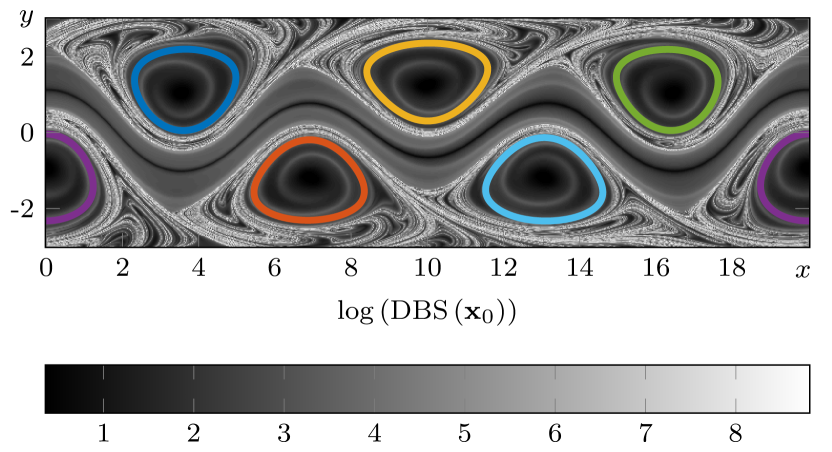
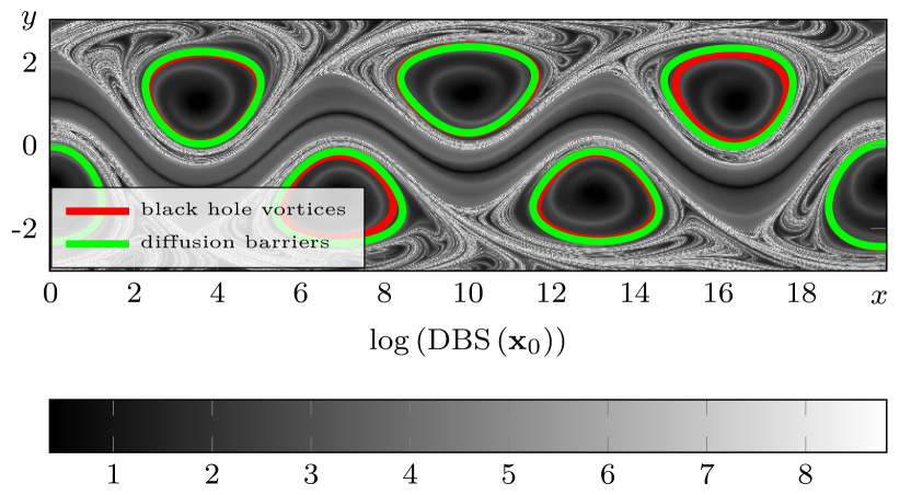
As a simple example, we consider here first the Bickley jet (39, 40), a kinematic model for a meandering jet surrounded by vortices. We use a quasiperiodically forced version of this velocity field, with parameter values taken from (41). Using the above refinements to the algorithm of (35), we show in Figure 4 predicted diffusion barriers for the time interval days in the Bickley jet with quasiperiodic time-dependence and anisotropic diffusion tensor .
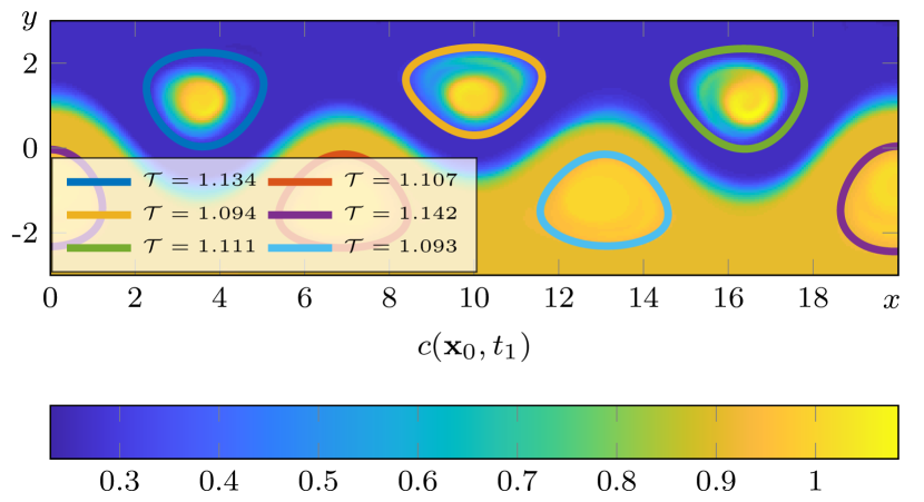
Almost all the diffusive vortex boundaries (red), identified at time as outermost closed orbits of the field are larger than any of the previously detected coherent sets in pure advection studies of this example (cf. (10) and Fig. 5). In flows with non-recurrent time dependence, invariants of the Cauchy–Green strain tensor and of its temporal average are expected to differ more, leading to an even more significant difference between LCSs and diffusion barriers (see Fig. 5). Diffusion noticeably erodes the scalar field inside closed barriers with higher values of the transport density . This confirms that our theory enables an a priori classification of diffusion barriers from purely advective calculations.
The trench of the field marks the core of the jet while ridges of the same field approximate backward-fronts (diffusive stable manifolds). The barriers we have located indeed prevail as organizing features of diffusive patterns, as shown in Fig. 6 in a diffusive simulation with Péclet number .
Our main example, discussed in the main text involves a two-dimensional unsteady velocity data set derived from AVISO satellite-observed sea-surface heights (SSH) under the geostrophic approximation (cf. (22) for details). As in (28), our computations cover a period of 90 days, ranging from to , over the longitudinal range and the latitudinal range containing the Agulhas leakage. This domain is covered by a regular 500x300 grid, on which we performed the steps detailed in Section 7 in the main text.
In addition to the results described in the main text, here we also show the final, evolved positions of material ring boundaries predicted solely from the satellite velocity field. Superimposed is the diffusing concentration to which the ring boundaries provide clear transport barriers (cf. Fig. 7).
Julia and MATLAB implementations of the algorithm given in Section 7 in the main text are available on request from the second author. Computation times (for the Julia version) on a 2.3 GHz Intel Core i5 (DualCore) notebook are about 50 seconds for the Bickley jet flow and about 90 seconds for the ocean flow example.
List of supporting animations:
- SA1.mov
-
Material advection of the closed Agulhas ring boundaries, identified at time as outermost closed diffusion barriers. Superimposed is the diffusing concentration.
- SA2.mov
-
Evolution of stochastic trajectories in the Lagrangian frame, released from inside and outside the four closed diffusion barriers bounding Agulhas rings.
- SA3.mov
-
Same as animation SA2.mov, but in the physical (Eulerian) frame.
References
- (1) Weiss JB, Provenzale A (2008) Transport and Mixing in Geophysical Flows. (Springer, Berlin).
- (2) Ottino J (1989) The Kinematics of Mixing: Stretching, Chaos and Transport. (Cambridge University Press, Cambridge).
- (3) Dinklage A, Klinger T, Marx G, Schweikhard L (2005) Plasma Physics - Confinement, Transport and Collective Effects. (Springer, Heidelberg).
- (4) Rosner D (2000) Transport Processes in Chemically Reacting Flow Systems. (Dover Publications).
- (5) Toda M (2005) Geometrical Structures of Phase Space In Multi-dimensional Chaos: Applications To Chemical Reaction Dynamics In Complex Systems. (John Wiley & Sons).
- (6) Peacock T, Dabiri J (2010) Focus issue on Lagrangian coherent structures. Chaos 20:017501.
- (7) Haller G (2015) Lagrangian Coherent Structures. Annu. Rev. Fluid Mech. 47:137–162.
- (8) Bahsoun W, Bose C, Froyland G (2014) Ergodic Theory, Open Dynamics, and Coherent Structures. (Springer, New York).
- (9) Peacock T, Froyland G, Haller G (2015) Focus issue on the objective detection of coherent structures. Chaos 25.
- (10) Hadjighasem A, Farazmand M, Blazevski D, Froyland G, Haller G (2017) A critical comparison of Lagrangian methods for coherent structure detection. Chaos 27:053104.
- (11) Press W, Rybicki G (1981) Enhancement of passive diffusion and suppression of heat flux in a fluid with time-varying shear. Astrophys. J. 248:751–766.
- (12) Knobloch E, Merryfield W (1992) Enhancement of diffusive transport in oscillatory flows. Astrophys. J. 401:196–205.
- (13) Thiffeault JL (2008) Scalar decay in chaotic mixing. Lect. Notes Phys. 744:3–35.
- (14) Tang X, Boozer A (1996) Finite time Lyapunov exponent and advection-diffusion equation. Physica D 95:283–305.
- (15) Thiffeault JL (2003) Advection-diffusion in Lagrangian coordinates. Phys. Lett. A 30:415–422.
- (16) Nakamura N (2008) Quantifying inhomogeneous, instantaneous, irreversible transport using passive tracer field as a coordinate. Lect. Notes Phys. 744:137–144.
- (17) Pratt L, Barkan R, Rypina I (2016) Scalar flux kinematics. Fluids 1:27.
- (18) Landau LD, Lifshitz E (1966) Fluid Mechanics. (Pergamon Press).
- (19) Gurtin M, Fried E, Anand L (2010) The Mechanics and Thermodynamics of Continua. (Cambridge University Press).
- (20) Liu W, Haller G (2004) Strange eigenmodes and decay of variance in the mixing of diffusive tracers. Physica D 188:1–39.
- (21) Castillo E, Luceno A, Pedregal P (2008) Composition functionals in calculus of variations. Application to products and quotients. Math. Models Methods Appl. Sci. 18:47–75.
- (22) Haller G, Beron-Vera FJ (2013) Coherent Lagrangian vortices: the black holes of turbulence. J. Fluid Mech. 731:R4.
- (23) Serra M, Haller G (2016) Objective Eulerian coherent structures. Chaos 26:053110.
- (24) Haller G, Beron-Vera F (2014) Addendum to ‘coherent Lagrangian vortices: the black holes of turbulence’. J. Fluid Mech. 751:R3.
- (25) Risken H (1984) The Fokker-Planck Equation: Methods of Solution and Applications. (Springer, New York).
- (26) Beal L, De Ruijter W, Biastoch A, Zahn R (2011) On the role of the agulhas system in ocean circulation and climate. Nature 472(7344):429–436.
- (27) Froyland G, Horenkamp C, Rossi V, van Sebille E (2015) Studying an agulhas ring’s long-term pathway and decay with finite-time coherent sets. Chaos 25(8):083119.
- (28) Hadjighasem A, Haller G (2016) Level set formulation of two-dimensional Lagrangian vortex detection methods. Chaos 26:103102.
- (29) Wang Y, Beron-Vera FJ, Olascoaga MJ (2016) The life cycle of a coherent lagrangian agulhas ring. J. Geophys. Res. [Oceans] 121:3944?3954.
- (30) Haller G, Hadjighasem A, Farazmand M, Huhn F (2016) Defining coherent vortices objectively from the vorticity. J. Fluid Mech. 795:136–173.
- (31) Friedman A (2013) Partial Differential Equations of Parabolic Type. (Dover Publications).
- (32) Logan J (1977) Invariant Variational Principles. Mathematics in Science and Engineering. Vol. 138, pp. 62–75.
- (33) Moser J (2003) Selected Chapters in the Calculus of Variations. (Springer, Basel).
- (34) Lewis J (1969) Homogeneous functions and Euler’s theorem. in: An Introduction to Mathematics. (Macmillan, London).
- (35) Hadjighasem A, Haller G (2016) Geodesic transport barriers in Jupiter’s atmosphere: A video-based analysis. SIAM Rev. pp. 69–89.
- (36) Karrasch D, Huhn F, Haller G (2015) Automated detection of coherent Lagrangian vortices in two-dimensional unsteady flows. Proc. R. Soc. A 471(2173):20140639.
- (37) Fyrillas M, Nomura K (2007) Diffusion and Brownian motion in Lagrangian coordinates. J. Chem. Phys. 126:164510.
- (38) Rößler A (2010) Runge–Kutta Methods for the Strong Approximation of Solutions of Stochastic Differential Equations. SIAM J. Numer. Anal. 48(3):922–952.
- (39) Del-Castillo-Negrete D, Morrison P (1993) Chaotic transport by rossby waves in shear flow. Phys. Fluids 5:948–965.
- (40) Rypina I, et al. (2007) On the Lagrangian dynamics of atmospheric zonal jets and the impermeability of the stratospheric polar vortex. J. Atmos. Sci. 64:3595–3610.
- (41) Hadjighasem A, Karrasch D, Teramoto H, Haller G (2016) Spectral clustering approach to Lagrangian vortex detection. Phys. Rev. E 93.