Unusual changeover in the transition nature of local-interaction Potts models

Abstract

A combinatorial approach is used to study the critical behavior of a $q$-state Potts model with a round-the-face interaction. Using this approach it is shown that the model exhibits a first order transition for $q>3$. A second order transition is numerically detected for $q=2$. Based on these findings, it is deduced that for some two-dimensional ferromagnetic Potts models with completely local interaction, there is a changeover in the transition order at a critical integer $q_{c}\leq 3$. This stands in contrast to the standard two-spin interaction Potts model where the maximal integer value for which the transition is continuous is $q_{c}=4$. A lower bound on the first order critical temperature is additionally derived.

I Introduction

The ferromagnetic $q$-state Potts model Potts and Domb (1952); Wu (1982) is one of the most widely studied models in statistical physics. At the core of the model is an interacting spin system with each spin possessing one out of $q$ possible states. The interaction consists of the simple rule that if the spins are monochromatic (have the same state) the energy level is lower than the case where they hold different states. Although the model is very easy to define, it is rich in interesting phenomena. A particular one that has been sparsely studied is the changeover from a second to a first order phase transition at a critical integer value $q_{c}$, or, in short, the changeover phenomenon.

Using an equivalence of the nearest-neighbor interaction model on the square lattice to a staggered ice-type model Temperley and Lieb (1971), Baxter Baxter (1973, 2013) obtained an exact nonzero expression for the latent heat when $q>4$. This expression has vanished at $q=4$. A vanishingly small jump in the free energy near $T_{c}$ has been found for $q\leq 4$. Based on these results, Baxter predicted that the model underwent a continuous (discontinuous) transition for $q\leq q_{c}$ ($q>q_{c}$) with $q_{c}=4$. His findings were believed to be lattice independent Nienhuis et al. (1979). Recently, Duminil-Copin and co-workers Duminil-Copin et al. (2016a, b) have rigorously confirmed Baxter’s predictions using the random cluster representation Fortuin and Kasteleyn (1972) of the nearest-neighbor interaction model.

Renormalization group (RG) theory has provided a useful framework to detect the changeover in the transition order. Nienhuis et al considered a generalized triangular lattice Potts model with additional lattice-gas variables and corresponding couplings, to control order-disorder in the renormalized system. Applying a generalized majority-rule Nienhuis et al. (1979); Domb (1977) to that model, the authors introduced a RG scheme for continuous values of $q$ which produced $q_{c}\approx 4.7$. Following Nienhuis et al. (1979); Nauenberg and Scalapino (1980), Cardy et al Cardy et al. (1980) proposed a system of differential RG equations describing the scale change of the ordering, thermal, dilution fields in the vicinity of a single multicritical point. The equations were derived based on the assumption that the ordering and thermal fields were relevant while the dilution field was marginal at the multicritical point. Investigating the equations near the multicritical point, the authors have found universal, presumably exact, parameters using previously known results Nijs (1979); Nienhuis et al. (1981).

It is known that some physical properties of all finite-range interaction models with the same dimensionality and symmetries are universal, that is, independent of the interaction details of one model or another. For instance, universality is manifested in the behavior of physical observables near criticality. One can then ask whether two dimensional local interaction ferromagnetic Potts models defined on various geometries and presenting the usual $q$-fold spontaneous symmetry breaking, in general mimic the changeover behavior of the standard pair-interaction model?

Some variants of the pair-interaction Potts model, with long but finite range interactions Gobron and Merola (2007) or with (exponentially) fast decaying inifinite-range interactions Chayes (2009), are known to exhibit a first order transition for $q\geq 3$. In another Potts model with the standard nearest-neighbor interaction, $r$ “invisible” states were added to the usual $q$ “visible” states Tamura et al. (2010); van Enter et al. (2011). The invisible states affected the entropy but did not alter the internal energy. It has been shown van Enter et al. (2011) that the transition is of first order for low $q$ ($q=2,3,4$), provided that $r$ is sufficiently large.

Based on Refs. Gobron and Merola (2007); Chayes (2009); Tamura et al. (2010); van Enter et al. (2011), the answer to the question raised above is apparently negative. Provided undergoing a continuous transition for some $q<3$, some of the systems Gobron and Merola (2007); Chayes (2009) display a changeover phenomenon at a critical integer $q_{c}<3$. It should be noted, however, that the models studied in Refs. Gobron and Merola (2007); Chayes (2009); Tamura et al. (2010); van Enter et al. (2011) have a complicated and somewhat “unnatural” interaction content.

A phase transition entails the emergence of a monochromatic giant component (macroscopic connected component taking up a positive fraction of the sites, hereby abbreviated as GC) whose existence becomes beneficial once the energy saved by the interactions overcomes the entropy cost. One may then ask what is the typical structure of such a monochromatic GC. In Schreiber et al. (2018) some of us used the correspondence between simple (non-fractal) and fractal-like clusters to the topology of ordered configurations in first and second order transitions, respectively, to show that for the round-the-face interaction Potts model on the square lattice, a changeover in the transition nature occurs at $q=4$. However, Monte-Carlo (MC) simulations Schreiber et al. (2018) of the model with $q=4$ resulting in a pronounced double-peaked shape of the pseudo-critical energy probability distribution function (PDF) Janke (1993), hints that a first-order transition is possible then.

In the present paper we develop a more rigorous approach, based on first principles, to study the phase transition of the round-the-face interaction Potts model. Using this approach, it is demonstrated on a simple “natural” model that satisfies the usual Potts $q$-fold broken symmetry, that within the class of $q$-state models with completely local interactions, a changeover phenomenon occurs at an integer value need not equal four. More precisely, we show that the model, defined on the honeycomb lattice, undergoes a first order transition for $q>3$. Under a few further conceivable assumptions related to the asymptotic number of hexagonal lattice animals (polyohexes) a first order transition is detected also for $q=3$. Extensive MC simulations Wang and Landau (2001) are performed for different values of $q$. For $q=2$, a second order transition is numerically observed. It follows that the honeycomb lattice model change over its transition nature at a critical value $q_{c}\leq 3$.

The rest of the paper is organized as follows. In section II we discuss the role of large scale lattice animals in determining the transition nature of the round-the-face interaction model. In section III we present and analyze in detail the results of Monte Carlo simulations. Our conclusions are drawn in section IV.

II Lattice Animals and the changeover phenomenon

Consider a ferromagnetic Potts model where the interaction involves $l$ spins residing at the vertices of an elementary cell (face) of a lattice with $N$ sites (e.g., $l=4$ for the square lattice). The model may be described by the Hamiltonian

$$-\beta{\cal H}=K\sum_{\text{faces}}\delta_{\sigma_{\text{face}}}\;,$$ (1)

where $\beta=1/k_{B}T$, $K=\beta J$ and $J>0$ is the ferromagnetic coupling constant (we will take from now on $k_{B}=J=1$ for convenience). The $\delta_{\sigma_{\text{face}}}$ symbol assigns $1$ if all the spins $\sigma_{\text{face}}:=\{\sigma_{1},\sigma_{2},...,\sigma_{l}\}$ on a given face simultaneously take one of the $q$ possible Potts states, and $0$ otherwise. The partition function of the Hamiltonian (1)

$$Z=\sum_{\{\sigma\}}\prod_{\text{faces}}(1+v\delta_{\sigma_{\text{face}}})\;,$$ (2)

where $v=e^{K}-1$, can take the form Wu (1982); Baxter (1973, 2013)

$$Z=q^{N}\sum_{G}q^{c(G)-\nu(G)}v^{f(G)}(1-1/q)^{\alpha(G)p(G)}\;,$$ (3)

where $G$ is a graph made of $c(G)$ clusters with a total number of $f(G)$ faces placed on its edges and $\nu(G)$ nodes. The total number of perimeter nodes is $p(G)$ and $\alpha(G)\leq 1$ is a positive proportionality factor.

Any cluster is either a lattice animal 978 (2017) or a lattice beast, that is, a collection of animals sharing joint nodes such that these animals are left unconnected. Let $b_{km}$ be the number of beasts with $k$ faces and $m$ sites. It is known Klarner (1967); Madras (1999) that the total number of animals of size $k$ on a two-dimensional periodic lattice takes the asymptotic form $\sum_{m}b^{\prime}_{km}\approx c\lambda^{k}k^{-1}$ (the prime refers to animal-like clusters), where $c$ is some constant. The total number of $k$-face beasts therefore asymptotically assumes $\sum_{m}b_{km}\sim\hat{\lambda}^{k}$ where $\hat{\lambda}\geq\lambda$.

A beast with holes contains finite clusters with boundaries colored differently than the surrounding bulk. In the following we refer to beasts with no holes. Consider a beast with $m/k\approx\rho$ where $\rho$ is the minimal asymptotic number of sites per face (e.g., for a perfect square on the square lattice with $m=(\sqrt{k}+1)^{2}$, $\rho=1$). Necessarily, this beast is simple. Identifying a simple beast with a boundary of size $B=o(N)$, its number of sites per face is no larger than $(m+\Delta m)/k$ with $m/k\approx\rho$ and $\Delta m=o(N)$, hence it approaches $\rho$ in the large $N$ limit. Simple combinatorics shows that the number of simple $k$-face beasts is bounded by $KN^{aB}$ for some constants $a,K$, i.e., sub-exponential in (large) $N$. It follows that for a given $\delta>0$ a family of (quasi)fractal beasts (QFs) with $m/k\approx\rho+\delta$, exponentially-growing at a rate $\mu\equiv\mu(\delta)$, is established. Making such a family of beasts monochromatic changes the entropy in the amount of

$$\Delta S = \ln\left(\mu^{k}/q^{m}\right)+\mbox{perimeter term}+\mbox{higher order terms}$$ (4)

$$= k\ln\left(\mu/q^{\rho+\delta}\right)+\theta k\ln(1-1/q)+o(N)\;,$$

where $\theta k$ is a fraction of $O(N)$ perimeter sites. Consequently, the change in the free energy $\Delta F=-k-T\Delta S$ (for large $k$) satisfies

$$\Delta F\geq-k(1-T\rho\ln q)-Tk\ln\left(\mu/q^{\delta}\right)\;.$$ (5)

Now, at $T^{\ast}=1/\rho\ln q$, the temperature at which the energy gain balances the entropy loss due to the formation of a simple GC (effectively associated with $\delta=0,\mu=1$ and $\theta=0$ in (4),(5)), $\Delta F\geq 0$ if $\mu/q^{\delta}\leq 1.$ This means that for $q\geq q_{s}$, where

$$q_{s}=\sup_{\delta}\mu^{1/\delta}\;,$$ (6)

it is disadvantageous for the system to occupy QFs at $T^{\ast}$. Instead, the system possesses a simple GC at that temperature and a first order transition is exhibited. Conversely, if the system undergoes a second order transition then for some $q<q_{s}$ and some $0<\delta\leq 2\rho$ there exist an exponential family $\mu$ such that $\mu/q^{\delta}>1$.

Note that in (5), a contribution generated by a macroscopic number of “small” clusters is ignored. To roughly estimate this contribution we consider the free energy of the disordered state $F=\langle E\rangle-TS$, where the entropy is bounded by $N\ln q$, and the mean energy is approximated by $\langle E\rangle\approx-\vartheta Np_{s}$ where $\vartheta N$ is the total number of faces of the small clusters and

$$p_{s}=\frac{qe^{K}}{qe^{K}+q^{\ell}-q}\;,$$ (7)

is the probability for a single face to be monochromatic with $\ell=2\rho+2$ being the number of spins in an interaction (e.g., $\ell=6$ for the honeycomb lattice). In evaluating $\langle E\rangle$ one can include additional terms accounting also for monochromatic pairs of faces etc. However, these can be seen to give smaller contributions. Adding $\langle E\rangle$ with $p_{s}^{\ast}$, the probability in (7), computed at $T^{\ast}$, or, at $e^{K}=q^{\rho}$, to the right-hand-side of (5) results (taking $\vartheta N=k$) in the approximated first order critical temperature

$$T_{c}\approx\frac{1-p_{s}^{\ast}}{\rho\ln q}\sim T^{\ast}-\frac{1}{q^{\rho+1}}\;.$$ (8)

In App. A the lower bound $\hat{T}=1/\ln(q^{\rho}+1)$ on $T_{c}$ is obtained. Indeed, $|T^{\ast}-\hat{T}|\gtrsim q^{-\rho-1}$ already for small $q$.

We focus now on the honeycomb lattice since for this lattice only “pure” animals survive (there are no beasts made of animals with joint nodes). Consider an animal with no holes. Let $n_{1},n_{2}$ and $n_{3}$ be the number of sites belonging to one, two and three faces, respectively. The total number of boundary sites is $b$. A simple counting gives

$$n_{1}+2n_{2}+3n_{3} = 6k\;,$$

$$n_{1}+n_{2}+n_{3} = m\;,$$

$$n_{1}+n_{2} = b\;.$$ (9)

One can easily verify that the minimal asymptotic number of sites per face is $\rho=2$. Expressing $b/k$ and $\delta+o(1)=m/k-2$ in terms of $n_{1},n_{2},n_{3}$ and noticing that $n_{1}=n_{2}+6$ result in

$$b/k\leq 2\delta+o(1)\;.$$ (10)

It is known Nienhuis (1982); Duminil-Copin and Smirnov (2012) that the connective constant of self-avoiding walks (SAWs) on the honeycomb lattice is $\mu_{c}=\sqrt{2+\sqrt{2}}$. The exponential number of animals of size $k$ in a family with a growth constant $\mu$ is bounded by the number of SAWs of length $\tilde{b}=\sup_{n_{1}}b$, i.e., $\mu^{k}\leq\mu_{c}^{\tilde{b}}$. With the help of (10) we thus obtain

$$\mu\leq\mu_{c}^{2\delta+o(1)}\;.$$ (11)

Combining (6) and (11) together it follows that $q_{s}\leq\mu_{c}^{2}\approx 3.4$. Consequently, the system undergoes a first order transition for $q>3$.

Indeed, our simulations indicate that a first order transition already occurs at $q=3$. Under a few plausible assumptions, this result can be analytically derived. First, define a snake to be an animal with boundary sites only ($n_{3}=0$), such that any of its faces (excluding the head and the tail) has two neighboring faces. Next, consider constrained SAWs tracing animals in a way that allows these walks to share three edges at most with any face along their travel. Consider all the faces with edges mutual to a given constrained walk and placed, say, to its left. It may occur that these faces construct a snake. Conversely, the single side boundary of any snake can be traced by a trajectory overlapping with no more than three edges per face. Thus, the number of snakes is no larger than the number of constrained walks. Noticing that snakes are animals associated with (maximal) $\delta=2$, we may write

$$\mu\leq\mu_{c}^{\varepsilon\delta/2},\ \delta\approx 2\;,$$ (12)

with $\varepsilon\leq 3$. Assuming that (6) is governed by quasi-snakes satisfying (12) and substituting $\varepsilon=3$ in (12) imply $q_{s}<3$ hence a first order transition for $q\geq 3$.

To conclude this section we point out that (10) holds also for the triangular and square lattices. This is shown (see App. B) using counting arguments similar to (II). It follows that since  (6) is governed by a family $\mu$ most likely dominated by animals large enough such that (11) is valid, the changeover phenomenon is a universal property of the round-the-face model.

III Monte Carlo simulations

In order to numerically support our predictions for the honeycomb lattice we perform Monte-Carlo simulations using the Wang-Landau Wang and Landau (2001) entropic sampling method. According to this method one hops between successive spin configurations with energies $E_{i}$ and $E_{j}$, respectively, with a transition probability $T_{i\to j}=\min\{1,\Omega(E_{i})/\Omega(E_{j})\}$ where $\Omega(E_{i})$ is an approximation to the density of states with energy $E_{i}$. At each visit to a state with energy $E_{i}$ the corresponding quantity $\ln\Omega(E_{i})$ is modified. We use lattices with linear sizes $5\leq L\leq 49$ and periodic boundary conditions are imposed. We focus on $q=2,3,4$. The specific heat maximum $C_{L}^{\max}$ is measured for each $L$ and finite size scaling (FSS) analysis is performed to these measurements. The location (temperature, $T_{L}$) of $C_{L}^{\max}$ serves as a definition to the pseudo-critical transition temperature.

A more sensitive measure, designed for first order transitions is $T_{L}^{W}$, the size-dependent temperature where $W_{o}$, the weight of the energy PDF in the ordered phase is $q$ times $W_{d}$, the weight in the disordered phase Janke (1993). To compute this quantity, an initial temperature is determined such that roughly $W_{o}/W_{d}\approx q$, where $W_{o},W_{d}$ are taken to be $\varphi(\epsilon_{\min}),1-\varphi(\epsilon_{\min})$, respectively, and $\varphi(\epsilon_{\min})$ is the cumulative distribution function computed at $\epsilon_{\min}$, the energy where there is a minimum between the peaks Janke (1993). The PDF is then iteratively calculated for increasing (decreasing) temperatures until convergence is achieved, that is, until

$$|W_{o}/W_{d}-q|<\tilde{\epsilon}\;,$$ (13)

is satisfied for some $\tilde{\epsilon}$.

For both $q=3,4$, using a sample of size $L=45$ and taking $\tilde{\epsilon}=5\times 10^{-3}$, a temperature increment $\Delta T=10^{-8}$ is needed to satisfy (13), while for $q=4$, $L=49$ and $\Delta T=10^{-8}$ convergence is attained for $\tilde{\epsilon}=10^{-3}$.

In Table 1 we summarize the quantities $T_{L}$ and $T_{L}^{W}$ together with the bounds $\hat{T}=1/\ln(q^{2}+1)$. Both measured temperatures reasonably agree with $\hat{T}$. Further simulations using larger samples, however, are needed to reliably estimate $T_{c}$.

	$L$	$T_{L}$	$T_{L}^{W}$	$\hat{T}$
$q=3$	$45$	$0.4420$	$0.4415(5)$	$0.4342(9)$
$q=4$	$45$ $49$	$0.3530$ $0.3534$	$0.3526(9)$ $0.3531(7)$	$0.3529(5)$

Table 1: Finite size lattice pseudo-critical temperatures $T_{L}$ and $T_{L}^{W}$ together with the lower bounds $\hat{T}$ on the first order critical points.

We next fit the specific heat maxima $C_{L}^{\max}$ with a power-law $C_{L}^{\max}\sim L^{\gamma}$ for $q=3,4$. In order to prune out finite size effects and systematically detect the FSS of large samples, we consider the maxima of the specific heat per site $C_{L}^{\max}/N,\ N=L^{2}$ and fit this observable with a power-law $C_{L}^{\max}/N\sim L^{-\nu}$ where $\nu=d-\gamma$.

The results of the numerical analysis are graphically captured in Fig. 1.

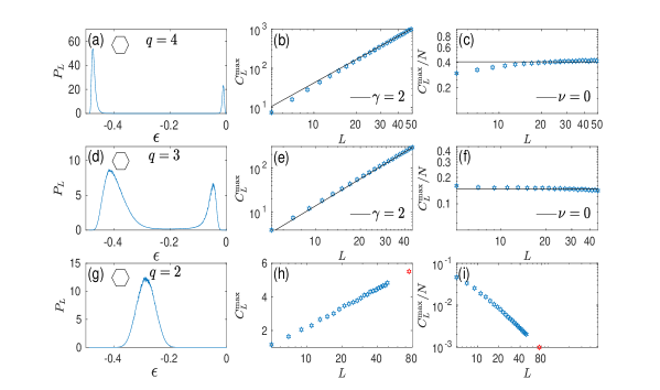
Figure 1: Energy pseudo-critical PDF and FSS of related observables for the honeycomb lattice. The PDF (computed for $L=45$), FSS of the specific heat maxima and FSS of the specific heat per site maxima are presented from left to right, respectively. The quantities described above are associated (from top to bottom) with $q=4,3,2$. The red symbols in (h),(i) represent the large sample ($L=75$) Metropolis based observables.

Fig. 1(a) shows the PDF at $T_{L}^{W}$ for q = 4 which displays a strong first-order performance for a rather small sample ($L=45$). In Fig. 1(b) $C_{L}^{\max}\sim L^{2}$ apparently obey the expected first order $C_{L}^{\max}\approx L^{d}$ scaling law, suggesting that we use sample sizes $L$ comparable with the correlation length. The first order nature is supported by a slowly varying $C_{L}^{\max}/N$ (Fig. 1(c)), indicating an expected first order asymptotic non-vanishing bahavior. Continuing with $q=3$ and Fig. 1(d), the typical pronounced double picked scenario for the PDF at $T_{L}^{W}$ is clearly observed, although this quantity apparently suffers from finite size effects, depicted mainly in the width of the peaks. Fitting $C_{L}^{\max}$ with $L^{2}$ as shown in Fig. 1(e), provides an indication for a first order behavior in the case of $q=3$. Similarly to the $q=4$ model, the nice fit with a zero-slope straight line observed in Fig. 1(f), suggests for an expected first order asymptotic constant term. The picture is substantially different for $q=2$. Unlike the dual peak shape characterizing the PDF of the former two models, the current model shows (Fig. 1(g)) a pronounced single peaked PDF (computed at $T_{L}$), indicating a continuous transition. Motivated by this qualitative difference it seems natural to expect for an Ising-like behavior when $q=2$, i.e., a logarithmic divergence of the specific heat, as captured by Fig. 1(h). Finally, as seen in Fig. 1(i), the pseudo-singularity of the specific heat per site decays with $L$, as expected from second order systems. Furthermore, the rapid decay hints that the $L^{-d}$ Ising scenario is likely to take place for larger samples.

In order to better apprehend the Ising-like nature of the $q=2$ model we employ the Metropolis Metropolis et al. (1953) method to calculate $C_{L}^{\max}$ and $C_{L}^{\max}/N$, using the energy histogram of a sample with $L=75$. The associated temperature $T_{L}=0.6549$ is extrapolated by fitting the WL data with the Ising form $|T_{L}-T_{c}|\propto L^{-1}$ where $T_{c}=0.6596$ $(L_{\min}^{\rm{best}}=11,\ \chi^{2}/\mbox{d.o.f.}=0.04/12,\ p\ \mbox{value}=4\times 10^{-6}$ Schreiber et al. (2018); Martin-Mayor (2007)). Indeed, as evident from Figs. 1(h),1(i), the FSS based on the WL simulations is preserved. Further analyses of Metropolis simulations on large scale and WL-based energy-dependent observables are provided in App. C.

IV Conclusions

The changeover phenomenon in local-interaction ferromagnetic Potts models is studied. The close link between the round-the-face interaction Potts model and two-dimensional lattice animals, applied to the honeycomb lattice, together with Monte-Carlo simulations, are used to derive $q_{c}\leq 3$. Specifically, numerical results and analytical considerations indicate a first order transition for $q=3$. If this was to be the case, there would be a changeover phenomenon at $q_{c}=2$.

Our results for $q_{c}$ stand in contrast to the well known result $q_{c}=4$ of the usual model Baxter (1973, 2013); Duminil-Copin et al. (2016b, a). Thus, first, by demonstrating on a natural local-interaction model a changeover phenomenon at a critical value $q_{c}<4$, we provide a deeper insight on this problem strengthening the realization that $q_{c}=4$ being universal is a false statement Gobron and Merola (2007); Chayes (2009); Tamura et al. (2010); van Enter et al. (2011). Second, our analytical and numerical analyses propose that the RG framework of Ref. Cardy et al. (1980) assuming a single multicritical point, does not capture a changeover phenomenon in multiple models. In other words, our study suggests that there may be multiple multicritical points were critical and tricritical branches terminate, keeping the thermal and ordering field relevant and the dilution field marginal at these points. Equivalently, our work may push the boundaries of the conventional ordering field, temperature, dilution picture Nienhuis et al. (1979); Cardy et al. (1980); Blöte et al. (2017), such that a new scaling field allowing for the variation of $q_{c}$ is introduced.

Appendix A A lower bound on the first order critical temperature

In the following we show that

$$\hat{T}=\frac{1}{\ln(q^{\rho}+1)}\;,$$ (14)

is a lower bound on $T_{c}$, the first order critical point.

Consider the partition function $Z_{g}$ associated with the giant component at the vicinity of $T_{c}$. Introducing the variables $f(G)=k,\ \nu(G)=m$ and taking $c(G)=1$ in (3), $Z_{g}$ takes the form

$$Z_{g}\propto q^{N}\sum_{m}b_{km}q^{-m}v^{k}\times\left(\rm perimeter\ terms\right)\;.$$ (15)

Assuming no holes, the number of simple beasts $\sum_{m}b_{km}$ is sub-exponential. The free energy per site is then governed by the single beast exponential terms and, taking $m=\rho k+o(N)$, reads

$$\phi = -T\ln\lim_{N\to\infty}Z^{1/N}$$ (16)

$$= \left\{\begin{array}[]{ll}-T\ln q+T\epsilon_{o}\ln(vq^{-\rho})&,v>q^{\rho}\\ -\hat{T}\ln q&,v=q^{\rho}\;,\end{array}\right.$$ (18)

where $\epsilon_{o}=-\lim_{N\to\infty}k_{o}(N)/N$ is the energy per site which in general depends on $v$, $k_{o}(N)$ maximizes $Z_{g}$ and $\hat{T}\equiv T(v=q^{\rho})$. Now at $v=q^{\rho}$ the free energy (16) is non-differentiable, making $\hat{T}$ a candidate for $T_{c}$. Suppose that $T_{c}=\hat{T}$. Then, $\phi(T_{c})>-1/\rho$, i.e., the free energy at the critical point is larger than the ground state energy which if of course impossible. This means that an entropy driven term generated by a macroscopic number of holes must be added to (16), making the assumption that holes are absent false and yields

$$T_{c}\geq\hat{T}\;.$$ (19)

Appendix B Eq. (10) is lattice independent

We generalize Eq. (10)

$$b/k\leq 2\delta+o(1)\;,$$ (20)

obtained for the honeycomb lattice, to the triangular and square lattices. The notations $k,m$ and $b$ refer to the number of faces, sites and boundary sites, respectively, of an arbitrary beast. The derivations are valid for beasts with no holes.

B.0.1 Triangular lattice

The total number of sites of any cluster on the triangular lattice can be decomposed into (non-zero) numbers $n_{1},n_{2},n_{3},n_{4},n_{6}$ of sites belonging to one, two, three, four, six faces, respectively (it is impossible to uniformly colour five faces with a joint vertex, as the face-interaction imposes that the sixth face sharing that vertex will have the same colour. Therefore $n_{5}=0$). Similarly to (10) in the main text we write

$$n_{1}+2n_{2}+3n_{3}+4n_{4}+6n_{6} = 3k\;,$$

$$n_{1}+n_{2}+n_{3}+n_{4}+n_{6} = m\;,$$

$$n_{1}+n_{2}+n_{3}+n_{4} = b\;.$$ (21)

Noticing that the minimal asymptotic number of sites per face on the triangular lattice is $\rho=1/2$ and expressing $b/k$ and $\delta+o(1)=m/k-1/2$ in terms of $n_{1},...,n_{6}$, we have that  (20) immediately follows if and only if

$$2n_{1}+n_{2}\geq n_{4}\;.$$ (22)

In order to prove (22) we first consider a single animal $a$. We notice that one gains a total curvature of $2\pi$ when travelling in six different directions along the animal’s perimeter. Non-zero contributions are attributed to crossing $n_{1a},n_{2a}$ and $n_{4a}$ vertices. A vertex of each type has a curvature of $2\pi/3,\pi/3$ and $-\pi/3$, respectively. We thus have

$$2n_{1a}+n_{2a}-n_{4a}=6\;.$$ (23)

We next observe that a beast is essentially made of $s$ animals interacting via $s-1$ vertices. Thus, the total number of sites of the beast, belonging to one, two and four faces is

$$n_{1} = \sum_{a}n_{1a}-2s+2\;,$$

$$n_{2} = \sum_{a}n_{2a}+s-1\;,$$

$$n_{4} = \sum_{a}n_{4a}\;,$$ (24)

respectively. Summing over (23) and using (B.0.1) lead to

$$2n_{1}+n_{2}-n_{4}=3s+3\;,$$ (25)

which completes the proof.

B.0.2 Square lattice

Let $n_{1},n_{2},n_{3}$ and $n_{4}$ be the number of sites belonging to one, two, three and four faces, respectively, of a given cluster on the square lattice. Then

$$n_{1}+2n_{2}+3n_{3}+4n_{4} = 4k\;,$$

$$n_{1}+n_{2}+n_{3}+n_{4} = m\;,$$

$$n_{1}+n_{2}+n_{3} = b\;.$$ (26)

On the square lattice there are $\rho=1$ sites per face for simple large clusters. Writing $\delta+o(1)=m/k-1$ and $b/k$ by means of $n_{1},...,n_{4}$ results in (20), iff

$$n_{1}\geq n_{3}$$ (27)

holds. To prove (27) we, again, first consider a single animal $a$. We see that any vertex on its perimeter with a non-zero curvature, belongs either to a single face or to three faces. A vertex of each type contributes $\pi/2$ and $-\pi/2$, respectively, to the total curvature of $2\pi$. Thus,

$$n_{1a}-n_{3a}=4\;.$$ (28)

Next we consider a beast with which can be decomposed into $s$ animals. Employing procedures similar to those described for the triangular lattice, we wind up with

$$n_{1}-n_{3}=2s+2\;,$$ (29)

which completes the proof.

Appendix C Energy-dependent observables and magnetization

We discuss additional numerical manifestations of the occurrence and nature of phase transitions on the honeycomb lattice. Some of them are remarkably captured by the specific heat and internal energy which are closely related to the first and second moments, respectively, of the energy PDF. The specific heat per spin is given by

$$c_{L}=L^{d}\beta^{2}(\langle\epsilon^{2}\rangle-\langle\epsilon\rangle^{2})\;,$$ (30)

and the internal energy is $\langle\epsilon\rangle$. The thermal averages $\langle...\rangle$ are taken with respect to the PDF

$$p_{L}(\epsilon)\propto g_{L}(\epsilon)e^{-\beta L^{d}\epsilon}\;,$$ (31)

and $g_{L}(\epsilon)$ is the density of states with energy $\epsilon$. Plots of the two observables are given in Fig. A.1.

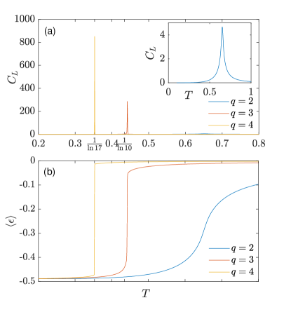
Figure A.1: Energy PDF first and second moment-dependent observables as a function of the temperature for $q=2,3,4$ and $L=45$. The bound $1/\ln(q^{2}+1)$ on the first order critical temperature is indicated in the cases of $q=3$ and $q=4$. (a) The specific heat $C_{L}$. A blow-up in the case of $q=2$ is given in the inset. (b) The internal energy $\langle\epsilon\rangle$.

Fig. A.1(a) shows the variation of the specific heat with temperature. While a clear sharp and narrow peak is observed at $q=3$ and $q=4$ (first order), a broad, two order of magnitude smaller (essentially hardly noticed on a uniform scale) peak, is seen when $q=2$. The latter scenario is indeed typical to second order transitions where large energy fluctuations are present on a relatively large energy scale. In Fig. A.1(b) we plot the internal energy against the temperature. A latent heat proportional to the ground state energy (per spin) of one-half, is evident for $q=3,4$. In the Ising-like case of $q=2$, however, the internal energy is a moderate monotonically increasing function of the temperature. Note also the nice proximity of the positions of both the peak and the jump in energy, to the approximated critical temperature $T_{c}\approx 1/(\ln q^{\rho}+1)$ (with $\rho=2$) for $q=3$ and, in particular, for $q=4$.

Another observable which presents a typical first order behavior when computed for the $q=4$ model is the magnetization at time (Monte-Carlo sweep) $t$ , given by

$$m(t)=\frac{qx(t)-1}{q-1}\;,$$ (32)

where $x(t)$ is the maximal fraction of spins which are simultaneously at the same Potts state. Indeed, since $q^{-1}\leq x(t)\leq 1$, (32) implies that $0\leq m(t)\leq 1$. We employ the Metropolis method to measure the magnetization (32). We also simulate the energy density according to (1).

In Fig. A.2(a) we plot the magnetization for a large sample ($L=100$) at the vicinity of $T^{\ast}$ for $q=4$.

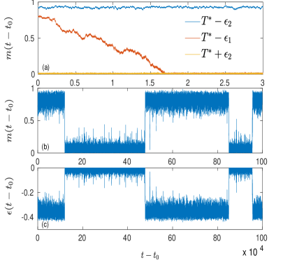
Figure A.2: Magnetization and energy density against time for the $q=4$ model on the honeycomb lattice, simulated at the vicinity of $T^{\ast}=(2\ln 4)^{-1}$. Two different samples with $L=100$ and $L=20$ are used. We let the system equilibrate starting from a totally ordered configuration, and translate the time frame by the equilibration time $t_{0}$. (a) $L=100$, $t_{0}=2000$, $\epsilon_{1}=0.001,\ \epsilon_{2}=0.01$ (b) $L=20$, $t_{0}=1000$, $T=T^{\ast}-0.025$ (c) $L=20$, $t_{0}=1000$, $T=T^{\ast}-0.025$ .

Note that $T^{\ast}-\hat{T}=(\ln 16)^{-1}-(\ln 17)^{-1}\approx 0.008$ so it is reasonable that the observed metastability at $T^{\ast}-\epsilon_{1}$ agrees with the expected metastability at $T_{L}\approx T^{\ast}-\epsilon_{1}\approx T_{c}$ satisfying the usual first order relation $|T_{c}-T_{L}|\propto L^{-d}$. When distorted in $\epsilon_{2}>\epsilon_{1}$ below (above) $T^{\ast}$, or, at temperatures smaller (larger) than $T_{c}$, the system rapidly relaxes to the ordered (disordered) state, respectively. Since relaxation times for large samples, when approaching $T_{c}$, are extremely long, we additionally simulate a small sample ($L=20$) near $T_{c}$ and plot the time dependent magnetization and energy density, in Fig. A.2(b) and Fig. A.2(c). As clearly observed in these figures, the large fluctuations enable the system to visit coexisting states in a reasonable time.

References

- Potts and Domb (1952) R. B. Potts and C. Domb, Mathematical Proceedings of the Cambridge Philosophical Society 48, 106 (1952).
- Wu (1982) F. Y. Wu, Reviews of Modern Physics 54, 235 (1982).
- Temperley and Lieb (1971) H. N. V. Temperley and E. H. Lieb, Proceedings of the Royal Society A: Mathematical, Physical and Engineering Sciences 322, 251 (1971).
- Baxter (1973) R. J. Baxter, Journal of Physics C: Solid State Physics 6, L445 (1973).
- Baxter (2013) R. J. Baxter, Exactly Solved Models in Statistical Mechanics (Dover Books on Physics) (Dover Publications, 2013).
- Nienhuis et al. (1979) B. Nienhuis, A. N. Berker, E. K. Riedel, and M. Schick, Physical Review Letters 43, 737 (1979).
- Duminil-Copin et al. (2016a) H. Duminil-Copin, V. Sidoravicius, and V. Tassion, Communications in Mathematical Physics 349, 47 (2016a).
- Duminil-Copin et al. (2016b) H. Duminil-Copin, M. Gagnebin, M. Harel, I. Manolescu, and V. Tassion, “Discontinuity of the phase transition for the planar random-cluster and potts models with ,” (2016b), arXiv:1611.09877 .
- Fortuin and Kasteleyn (1972) C. Fortuin and P. Kasteleyn, Physica 57, 536 (1972).
- Domb (1977) C. Domb, Phase Transitions and Critical Phenomena. Volume 6 (Academic Press, 1977).
- Nauenberg and Scalapino (1980) M. Nauenberg and D. J. Scalapino, Physical Review Letters 44, 837 (1980).
- Cardy et al. (1980) J. L. Cardy, M. Nauenberg, and D. J. Scalapino, Physical Review B 22, 2560 (1980).
- Nijs (1979) M. D. Nijs, Physica A: Statistical Mechanics and its Applications 95, 449 (1979).
- Nienhuis et al. (1981) B. Nienhuis, E. K. Riedel, and M. Schick, Physical Review B 23, 6055 (1981).
- Gobron and Merola (2007) T. Gobron and I. Merola, Journal of Statistical Physics 126, 507 (2007).
- Chayes (2009) L. Chayes, Communications in Mathematical Physics 292, 303 (2009).
- Tamura et al. (2010) R. Tamura, S. Tanaka, and N. Kawashima, Progress of Theoretical Physics 124, 381 (2010).
- van Enter et al. (2011) A. C. D. van Enter, G. Iacobelli, and S. Taati, Progress of Theoretical Physics 126, 983 (2011).
- Schreiber et al. (2018) N. Schreiber, R. Cohen, and S. Haber, Physical Review E 97 (2018).
- Janke (1993) W. Janke, Physical Review B 47, 14757 (1993).
- Wang and Landau (2001) F. Wang and D. P. Landau, Physical Review Letters 86, 2050 (2001).
- 978 (2017) Handbook of Discrete and Computational Geometry (Discrete Mathematics and Its Applications) (Chapman and Hall/CRC, 2017).
- Klarner (1967) D. A. Klarner, Journal canadien de mathématiques 19, 851 (1967).
- Madras (1999) N. Madras, Annals of Combinatorics 3, 357 (1999).
- Note (1) Travelling along the perimeter, every vertex contributes a curvature of and every vertex contributes a negative curvature . Since the total curvature is , we have that .
- Nienhuis (1982) B. Nienhuis, Physical Review Letters 49, 1062 (1982).
- Duminil-Copin and Smirnov (2012) H. Duminil-Copin and S. Smirnov, Annals of Mathematics 175, 1653 (2012).
- Note (2) Other animals with containing junctions, each branches into three snakes, can be treated as if they were sole snakes, provided the number of junctions is .
- Metropolis et al. (1953) N. Metropolis, A. W. Rosenbluth, M. N. Rosenbluth, A. H. Teller, and E. Teller, The Journal of Chemical Physics 21, 1087 (1953).
- Martin-Mayor (2007) V. Martin-Mayor, Physical Review Letters 98 (2007).
- Blöte et al. (2017) H. W. J. Blöte, W. Guo, and M. P. Nightingale, Journal of Physics A: Mathematical and Theoretical 50, 324001 (2017).
- Note (3) The quantities and correspond to the number of sites of animal belonging to one, two and four faces, respectively.
- Note (4) In practice we calculate moments of the distribution associated with , with , and rescale them properly.