Monitoring currents in cold-atom circuits

Abstract

Complex circuits of cold atoms can be exploited to devise new protocols for the diagnostics of cold-atoms systems. Specifically, we study the quench dynamics of a condensate confined in a ring-shaped potential coupled with a rectilinear guide of finite size. We find that the dynamics of the atoms inside the guide is distinctive of the states with different winding numbers in the ring condensate. We also observe that the depletion of the density, localized around the tunneling region of the ring condensate, can decay in a pair of excitations experiencing a Sagnac effect. In our approach, the current states of the condensate in the ring can be read out by inspection of the rectilinear guide only, leaving the ring condensate minimally affected by the measurement. We believe that our results set the basis for definition of new quantum rotation sensors. At the same time, our scheme can be employed to explore fundamental questions involving dynamics of bosonic condensates.

I Introduction

Nowadays, cold-atoms systems provide a tunable and flexible platform for studying quantum liquid behavior Leggett (1991). With the advances in quantum technology, remarkable progress has been achieved in the field. Concomitantly, cold-atoms systems have provided new tools, devices and perspectives to explore other branches of physics. And lying deep in this framework is a new field of atomtronics Seaman et al. (2007); Amico et al. (2005, 2017). This field seeks to realize atomic circuits where ultracold atoms are manipulated in a versatile laser-generated or magnetic guides. An important goal of the field is to enlarge the scope of the cold-atoms quantum simulators to study fundamental aspects of quantum coherent systems. At the same time, atomtronics aims at fabrication of new quantum devices and sensors with enhanced control and flexibility, by exploiting special features of the neutral cold-atoms quantum fluid Barrett et al. (2014); Arnold et al. (2006); Navez et al. (2016); Dumke et al. (2016).

There has been much interest in the simple circuit made of a bosonic condensate flowing in ring-shaped guides and pierced by an effective magnetic field Dalibard et al. (2011); Wright et al. (2013); Ramanathan et al. (2011); Ryu et al. (2013); Eckel et al. (2014); Yakimenko et al. (2015); Eckel et al. (2014); Hallwood et al. (2006); Solenov and Mozyrsky (2010); Amico et al. (2014); Aghamalyan et al. (2015, 2016, 2013); Mathey and Mathey (2016); Haug et al. (2018). We note, however, that the recent progress in the field allows us to access richer scenarios. Indeed, condensates can be loaded in basically arbitrary potentials with micron-scale resolution Zupancic et al. (2016); Haase et al. (2017). In addition, such potentials can be changed in shape and intensity at time scales of tens to hundreds microseconds, and therefore opening the way to modify the features of the circuit in the course of the same experiment (typically involving tens of milliseconds) Gauthier et al. (2016); Liang et al. (2009); Muldoon et al. (2012); Henderson et al. (2009). Remarkable advances on the flexibility and control of cold-atoms quantum technology, in turn, has opened up exciting possibilities for atomtronics. First, micro-fabricated integrated circuits of cold atoms can be feasibly realized. Second, the very shape and functionality of the circuit can be changed dynamically during its operation in a virtually continuous way.

Here, we study an integrated atomtronic circuit to realize new protocols for the manipulation of quantum fluids in complex networks of cold atoms. Schematically, the circuit is assumed to be divided into two distinct but coupled parts: ’primary’ and ’secondary’. We assume that the quantum fluid operates in the primary part of the circuit. Then we ask: Is it possible to gain information on the primary part by manipulating solely the secondary circuit? To answer this question, we study the dynamics of a simple setting: A bosonic condensate flowing in a ring-shaped guide tunnel-coupled to a rectilinear quantum well. In our circuit, the primary part is the ring-shaped condensate; the secondary part is the rectilinear guide. We see that the different current states in the ring correspond to distinctive dynamics of the condensate in the guide. Such a protocol could then be used to read out the current states in a quasi-continuous way, being limited mainly by the quality of the achieved BEC that operates in the primary circuit.

II The Circuit Structure

The circuit is made of a two-dimensional ring-shaped condensate coupled to a two-dimensional rectilinear quantum well of finite length. To paint a well-resolved circuit, we consider sharp potentials defined by step functions. The ring potential has radius $R$ and width $w$ centered at point $(x_{r},y_{r})$ and is defined with function $V_{r}(x,y)=-U_{0}$ when $R-\frac{w}{2}<r<R+\frac{w}{2}$ and is zero elsewhere. Here $r=\sqrt{(x-x_{r})^{2}+(y-y_{r})^{2}}$ and $U_{0}$ is the depth of the potential. A nearly resonant tunneling between the ring and waveguide is achieved for waveguide and ring with the same width $w$ and depth $U_{0}$. The waveguide potential, placed at distance $y_{g}$ from the $x$ axis, is defined as $V_{g}(x,y)=-U_{0}$ when $y_{g}-\frac{w}{2}<y<y_{g}+\frac{w}{2}$ and is zero elsewhere (Fig. 1).

We assume that the dynamics of the BEC is governed by Gross-Pitaevskii equation (GPE) and we write, in terms of dimensionless quantities,

$$\begin{aligned} &i\partial_{\tilde{t}}\tilde{\psi}(\tilde{\vec{r}},\tilde{t})=\\ &\left((-i\tilde{\vec{\nabla}}-\tilde{\vec{A}}(\tilde{\vec{r}}))^{2}+\tilde{V}(\tilde{\vec{r}})+N\tilde{u}|\tilde{\psi}(\tilde{\vec{r}},\tilde{t})|^{2}\right)\tilde{\psi}(\tilde{\vec{r}},\tilde{t}),\end{aligned}$$ (1)

where the dimensionless quantities are: $\tilde{\vec{r}}=k\vec{r}$, $\tilde{t}=\omega t$, $\tilde{\vec{\nabla}}=(\partial_{x}\hat{x}+\partial_{y}\hat{y})/k$, $\tilde{V}=V/E$, $\tilde{u}=2mu/\hbar^{2}$ and $\tilde{\psi}=\psi/k$ ($m$ is the mass of particles and $\hbar$ is the reduced Planck constant). The recoil energy $E=\hbar^{2}k^{2}/(2m)$, $k^{-1}=w/\pi$ and $\omega^{-1}=\hbar/E$ serve as the units of the energy, length and time, respectively. With our choice of the scaling units $\tilde{w}=kw=\pi$. The parameter $u=\frac{4\pi\hbar^{2}}{m\delta}a_{s}$ is the strength of the interaction in a two-dimensional system with s-wave scattering length $a_{s}$ and $3$D-to-$2$D scaling factor $\delta$.

The two-dimensional vector $\tilde{\vec{A}}=\vec{A}/(\hbar k)$, with $\vec{A}(\vec{r})=\frac{B}{2}(-(y-y_{r})\hat{x}+(x-x_{r})\hat{y})$, is the artificial gauge field resulting in an effective magnetic field with strength $\tilde{B}=B/(\hbar k^{2})$ in $\hat{z}$ direction, and flux $\Phi=B\pi r^{2}$. With $\Phi_{0}=h$ being the the flux quantum, the winding number for the atoms at radius $r$ from the center of the ring reads as $\Omega=\text{int}(\Phi/\Phi_{0})=\text{int}(\tilde{B}\tilde{r}^{2}/2)$. Finally, we consider normalized (scaled and non-scaled) wavefunction, $\int d\vec{r}~{}|\psi|^{2}=1$, in the computational space and a total number of particles $N$. Hereafter, we will work with dimensionless quantities and scaled GPE (1) while dropping the tilde from the notation for convenience.

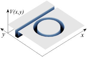
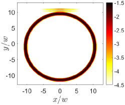
Figure 1: Top: schematic drawing of the circuit of cold atoms consisting of a ring-shaped trap and a rectilinear waveguide in $x$ direction. The atoms are absorbed at the two ends of the waveguide. Bottom: the logarithm of the atomic density in the system when some atoms have tunneled from ring to waveguide. We consider a ring potential with width $w$ and radius $R=10.5w$ in a computational space spanned over $-20w\leq x\leq 20w$ and $-15w\leq y\leq 15w$. In $x$ direction, a layer with the width $\Delta=5w$ is dedicated to ABC in both sides and therefore, the physical space is limited to $-15w<x<15w$. The ring is centered at $(x_{r},y_{r})=(0,-w)$ and the waveguide, with the same width as the ring, is located at $y_{g}=10.7w$. For such a ring, artificial magnetic field strengths of $B\pi^{2}=0,\pm 0.02,\pm 0.04,\pm 0.06$ result in winding numbers $\Omega=0,\pm 1,\pm 2,\pm 3$, respectively. We also consider an initial total particle number of $N=6\times 10^{5}$. Other parameters vary from case to case and their values are given when required. In the example presented here, the ring potential and the waveguide have same width $w$ and depth $U_{0}=20$. Atoms are stationary inside the ring ($\Omega=0$) and the atom-atom interaction strength is $u=2\times 10^{-4}$.

The atoms, which tunnel from the ring into the waveguide, spread in all directions and could reflect from a physical or computational boundary. Here we are interested in the case where atoms flow freely in the $x$ direction inside the waveguide. This scenario represents a physical system in which the atoms are absorbed, by detectors for instance, placed at the two ends of the waveguide or one in which the waveguide is sufficiently long so that there is no reflection in $x$ direction for the duration of observation. For this purpose we will apply absorbing boundary condition (ABC) in $x$ direction, minimizing the atoms’ reflection from the endpoints of the guide.

Indeed, there are different methods to apply ABC. Here we use a common method that makes use of an extra damping potential applied in a layer from the boundaries Jüngel and Mennemann (2010); Antoine et al. (2013): the absorbing potential is equal to zero in the physical region where $x_{L}<x<x_{R}$ and is defined as $V_{ABC}=\frac{-iV_{0}}{\Delta^{2}}(x-x_{L/R})^{2}$ when $x_{L}-\Delta\leq x\leq x_{L}$ or $x_{R}\leq x\leq x_{R}+\Delta$. Here, $V_{0}$ is the strength of the absorbing potential and $\Delta$ is the width of the solely-computational region in which ABC is applied. We do not apply any ABC in $y$ direction. We note that the ABC is applied only during the real time evolution while for imaginary time evolution (used to compute the ground state of the system) the layers beyond $x_{R}$ and $x_{L}$ are treated as the usual computational and physical space. The waveguide potential $V_{g}(x,y)$ is also defined for $x_{L}-\Delta\leq x\leq x_{R}+\Delta$.

III Results

We assume that the BEC is initially in the ground state corresponding to a circulating state of the atoms in the ring-shaped potential. Then, the gauge potential is switched-off and the trapping potential is quenched in such a way that the initially empty waveguide is turned on, next to the ring-shaped condensate. The atoms then tunnel from the ring into the waveguide.

Starting from the ground state of the atoms SupMat inside the ring potential with the depth $U_{0}=20$ and atom-atom interaction strength $u=2\times 10^{-4}$, for $\Omega=0,\pm 1,\pm 2,\pm 3$ and an ABC with $V_{0}=20$, we let the atoms tunnel from the ring into the waveguide which has the same depth and width. We specifically monitor three quantities inside the waveguide in time: the total number of atoms $N_{tot}=N\int dy\int dx|\psi(x,y,t)|^{2}$, the net flux of particles in $x$ direction $\int\int J_{x}=\int dy\int dxJ_{x}(x,y,t)$ where $J_{x}=-iN(\psi^{*}\partial_{x}\psi-\psi\partial_{x}\psi^{*})$ is the $x$ component of the atomic current, and finally, the position of center of mass in $x$ direction $\langle x\rangle=\int dy\int dx\psi^{*}(x,y,t)x\psi(x,y,t)$. All integrals are taken over the waveguide area.

Notice that, largely due to atom-atom interaction inside the ring, the geometric resonance between ring and guide may be lifted. Accordingly, we find that density profile of the atoms in $y$ direction of the waveguide clearly displays that first excited state in the waveguide with energy $E_{2}$ (bottom panel in Fig. 1) is occupied.

Following the dynamics of the atoms inside the waveguide, we do not observe any reflection from the boundaries in $x$ direction. However, the distribution of the atoms in $x$ direction is not continuous in time due to fluctuation of the number of atoms which tunnel from the ring into the waveguide. For all $\Omega$, we observe very similar number of atoms inside the waveguide (top panel in Fig. 2) indicating very similar tunneling rates (chemical potential $\mu$ in the ring has a very weak dependence on $\Omega$). Nevertheless, the current state inside the ring can be clearly read-out by looking at the imbalance between the right- and left-moving atoms as well as the center of mass position of the atomic density in the waveguide (middle and bottom panels of Fig. 2). While the sign of these quantities reveals the direction of rotation inside the ring, their absolute value can be used to probe the magnitude of the winding number.

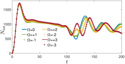
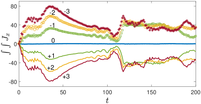
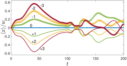
Figure 2: Dynamics of the total number of atoms $N_{\text{tot}}$ (top), the net particle flux in $x$ direction $\int{dx}\int{dy}J_{x}$ (middle) and the $x$ component of the center of mass of atomic cloud $\langle x\rangle$ (bottom) inside the waveguide, for non-rotating, $\Omega=0$, and rotating cases with $\Omega=\pm 1,\pm 2,\pm 3$. Value of $\Omega$ is indicated next to the corresponding curve in the middle and bottom panels. The ring potential and the waveguide have same width $w$ and depth $U_{0}=20$. Atom-atom interaction strength is $u=2\times 10^{-4}$ and ABC potential strength is $V_{0}=20$.

By inspection of Fig. 2, we notice a marked dip (around $t\sim 110-120$) in all plotted quantities. Such a feature traces back to a specific collective phenomenon occurring in the ring condensate: The tunneling process results in perturbation of the density of the condensate. Such a perturbation decays in a pair of density modulations which counter-propagate along the ring with negligible dispersion; given the very small magnitude of the perturbations, the excitations can be of phononic-type. Analyzing our results further, we see that the dip occurs shortly after the time at which the density modulations recombine around the tunneling region. For the non-rotating case the counter-propagating excitations with same frequency move with same speed to meet again at the same point where they were produced. For the flowing currents, instead, the frequency of excitations, and therefore the velocity of the density perturbations, are affected by Doppler effect SupMat ; Kumar et al. (2016), implying that the recombination point of the density perturbations is dragged along the superfluid current.

A simple Bogoliubov analysis of the idealized $1d$ ring condensate SupMat gives results which quantitatively agree with the numerical outcome. In particular, the modulation of the density propagate as $\delta|\psi|^{2}\propto\cos(q\phi\mp\omega^{\pm}t)$ where $\phi$ is angular coordinate along the ring and $q$ is the angular wavenumber of excitation. Here, $\omega^{\pm}=\omega_{0}\pm 2q\Omega/R^{2}$ are the enhanced and reduced frequencies (due to Doppler effect) of the two counter-propagating excitations and $\omega_{0}$ is the frequency of excitations in absence of rotation. The density perturbations produced by these excitations then travel with enhanced and reduced velocities $v^{\pm}=v_{0}\pm\Omega/R$, with $v_{0}$ being the velocity of density perturbations in absence of rotation, and reach their original place at times $T^{\pm}$, where $T^{+}<T^{-}$. We note that in Fig. 2, for $\Omega=\pm 2$ and $\pm 3$, there are two dips in $N_{\text{tot}}$ around the time $t\approx 120$ which indicate the time difference between the arrival of the fast and slow moving density perturbations at the tunneling point. This time difference has not been resolved in our numerical data for $\Omega=\pm 1$ due to the finite length of the density perturbations and small velocity shift. However, the dip in $N_{tot}$ for this case is shallower and wider than the one of non-rotating case. It is remarkable that such a Doppler effect of the excitations implies clear signatures in all quantities measured in the waveguide. As a result of the Doppler shift, the meeting point of the density perturbations is dragged along the supercurrent and when the perturbations meet around the tunneling region for the first time at $t=\pi R/v_{0}$ there is a Sagnac phase-shift of $k_{q}\omega_{s}{\cal{A}}/v_{0}$ Anderson et al. (1994). Here $k_{q}=q/R$ is the wavenumber of the excitations, ${\cal{A}}$ is the area of the circle and $\omega_{s}=2\Omega/R^{2}$ is the angular velocity of the supercurrent.

After the density perturbations reach back to the tunneling point the atoms’ distribution in waveguide becomes more complicated: The rotating states are still detectable from non-rotating state through the asymmetry in the net particle flux in the waveguide given by $\int{dx}\int{dy}J_{x}$; the states with different winding numbers, however, seem not to be distinguishable through the quantities shown in Fig. 2. Such time depends on the interaction strength through the group velocity of the rotating density perturbation (see SupMat for details). Therefore, with weaker interactions, the maximum time for which the rotating states are well-differentiated from each other is extended. On the other hand, the interaction reshuffles the configuration of the energy levels (through the chemical potential of ring condensate), affecting in turn the ring-guide tunneling rate.

Table 1 summarizes the difference between the chemical potential of atoms in the ring and three lowest discrete energy levels in the waveguide for three different values of atom-atom interaction strength $u$. Three top panels of the Fig. 3 show the total number of particles inside the waveguide for the rotating states with $\Omega=1$ and the three different values of the interaction strength displayed in the Table 1. We observe that the highest resonance case, with $u=2\times 10^{-4}$, corresponding to the highest tunneling rate, is characterized by a ‘clean’ time dependence. For larger detuning, in contrast the tunneling is much more erratic. This behavior suggests that, while the off-resonant ring-guide tunneling involves different frequencies, the near-resonant tunneling involves mostly a single level (the resonant one). Indeed, we see that it is the second discrete state (due to confinement in $y$ direction) to be involved in this case (bottom panel of Fig. 3). We note that, despite the small number of atoms in the waveguide for the off-resonant cases, the asymmetry due to rotation is still observed in the quantities plotted in Fig. 4.

$u$	$\mu$	$\mu-E_{1}$	$\mu-E_{2}$	$\mu-E_{3}$
$1\times 10^{-4}$	$-18.11$	$1.13$	$-1.15$	$-4.89$
$2\times 10^{-4}$	$-17.07$	$2.17$	$-0.11$	$-3.85$
$4\times 10^{-4}$	$-15.12$	$4.12$	$1.84$	$-1.9$

Table 1: The difference between the chemical potential of atoms in the ring $\mu$ and three lowest energy levels inside the waveguide for three different values of the atom-atom interaction strength $u$. All other parameters are the same as those in Fig. 2. Rotation does not change the first two decimal digits of the $\mu$ given here. The case with $u=2\times 10^{-4}$ has the highest resonance with the second level inside the waveguide.

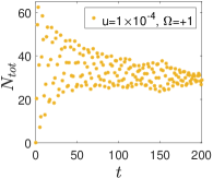
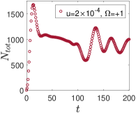
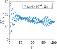
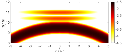
Figure 3: Three top panels: the total number of particles inside the waveguide in time, for the rotating states with $\Omega=+1$ and three different values of the atom-atom interaction strength $u$. The ring potential and the waveguide have same width $w$ and depth $U_{0}=20$ and the state in the ring with $u=2\times 10^{-4}$ (top-right panel) is in better resonance with the energy levels of the waveguide compared to other cases. ABC potential strength is $V_{0}=20$. Bottom panel: the logarithm of the atomic density in the waveguide and top side of the ring in vicinity of waveguide at time $t=13$ for the case with $\Omega=+1$ and $u=2\times 10^{-4}$. The density profile in $y$ direction inside the waveguide indicates that the second discrete level is occupied as expected.

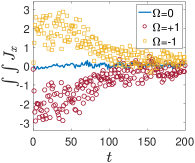
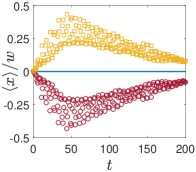
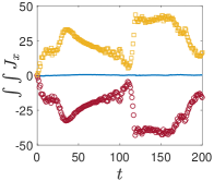
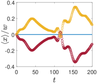
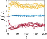
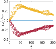
Figure 4: Dynamics of the net particle flux in $x$ direction $\int{dx}\int{dy}J_{x}$ (left panels) and the $x$ component of the center of mass of atomic cloud $\langle x\rangle$ (right panels) inside the waveguide, for three different values of the atom-atom interaction strength $u=1\times 10^{-4},~{}2\times 10^{-4}$ and $4\times 10^{-4}$ from top to bottom. Other parameters are the same as those in Fig. 3. The blue/solid lines correspond to the case with $\Omega=0$, the red/dark circles to $\Omega=+1$ and the yellow/light squares to $\Omega=-1$.

The resonant cases correspond to a large number of atoms tunneling from the ring to the waveguide, causing a substantial decrease of the density in the ring condensate. Indeed, the resonance condition can be controlled by tuning the waveguide’s parameters.

IV Notes on Experimental Implementation

Here we briefly discuss the feasibility of the proposed system in the experiment.

First we would like to mention that the step-function potentials are considered in this work for convenience in order to make it easier to tune the distance between the ring potential and the waveguide. Even though with the use of new technologies, such as SLM, fabrication of versatile forms of optical potentials has been made possible, we emphasis that what actually matters is the tunneling rate between the ring potential and the waveguide. Therefore, depending on the experimental setup, either the distance or the resonance between the energy levels of the two potentials can be used to control the tunneling rate. The resonance can also be controlled by either the depth or width of each potential. One could imagine that tuning and changing the geometrical parameters of the rectilinear waveguide is more convenient compared to changing the parameters of the ring potential.

Second point to consider is the ratio of the ring’s radius $R$ with respect to its width $w$. In this work we have considered a rather tight ring potential such that, for all values of the gauge field which are used, only one winding number is permitted in the ring. In other words, the winding number does not change from the inner radius to the outer radius of the ring. This condition is imposed mainly to avoid complications in numerical simulations. The aim has been to avoid excitation of unwanted states with higher winding numbers. Depending on the method used in the experiment to bring the atoms into rotation the $R/w$ ratio may not be of any concern.

As for the measurement time restrictions, if we consider ${}^{87}Rb$ atoms, for instance, in a ring potential with a width $w=1~{}\mu m$, the unit of time becomes $\omega^{-1}\approx 277.45~{}\mu s$. This means that the measurement must be performed within a time of $t\approx 100~{}\omega^{-1}\approx 27.7~{}ms$. We have also worked with dimensionless atom-atom interaction strengths $\tilde{u}=1,~{}2,~{}4\times 10^{-4}$ which are equivalent to scaled scattering lengths $a_{s}/\delta=4,~{}8,~{}16\times 10^{-6}$ for ${}^{87}Rb$ atoms. In a rough approximation the $3$D-to-$2$D scaling factor $\delta$ is equal to the size of the system in the transverse ($z$) dimension petrov2001 . Therefore, for a system with tight confinement in third dimension these values of $\tilde{u}$ represent very weak interactions.

V Conclusion

We provided a numerical analysis of the quench dynamics of a specific atomic circuit made of a ring-shaped bosonic condensate coupled with a rectilinear waveguide of finite length. We demonstrated that both magnitude and the direction of the current flowing through the ring can be detected through the inspection of the very small number of atoms tunneling from the ring into the waveguide. The protocol we conceived is minimally destructive on the ring condensate and allows to carry-out the measurements of the flowing states in a virtually continuous way while the ring operates. Interestingly enough, we find that the dynamics in the circuit is characterized by a peculiar effect: the depletion of the condensate density, caused by the ring condensate-waveguide tunneling, decays into a pair of phonon-type excitations. These excitations meet again, after they have traveled along the loop, in a position that is fixed by the Doppler effect induced by the persistent current and characterized by a Sagnac phase shift. Such effect plays a key role for the read-out protocols. At the same time, it could be exploited to access the predictions implied in the quasi-particles decay in Bose condensates Beliaev (1958); Giorgini (1998); Tan et al. (2010); Ristivojevic and Matveev (2016); Ozeri et al. (2005). In particular the crossover in the spatial dimension (from $3d$ down to $1d$) and interaction can be explored. In addition, by playing with the ring-guide coupling, one could produce density excitations of more substantial magnitudes (soliton-like), with different pair formation mechanism Kivshar and Malomed (1989); Nguyen et al. (2014). We believe that our work will play an instrumental role for the diagnostics of cold-atoms systems with non-trivial winding numbers. We have also shown that fundamental physics is implied in the dynamics of the system. Finally, our circuit provides the basis for a new architecture of rotation sensors.

VI Acknowledgments

We would like to acknowledge fruitful discussions with B. Grémaud, T. Haug and C. Miniatura. This research is supported by the National Research Foundation, Prime Minister’s Office, Singapore and the Ministry of Education-Singapore, under the Research Centres of Excellence programme and Academic Research Fund Tier 2 (Grant No. MOE2015-T2-1-101). The computational work for this article was mainly performed on resources of the National Supercomputing Centre, Singapore (https://www.nscc.sg). The Grenoble LANEF framework (ANR-10-LABX-51-01) is acknowledged for its support with mutualized infrastructure.

Appendix A Numerical method

To compute the dynamics of the system governed by equation (1) of the main text, in real or imaginary time, we use a generalized version of the Split-Step Method developed in Bao and Wang (2006), where a gauge field of the form $\vec{A}(x,y)=A_{x}(y)\hat{x}+A_{y}(x)\hat{y}$ is considered. This method covers the gauge field that we have used in this work as long as $B$ is constant everywhere. For the numerical results presented in this paper, we first compute the ground state of the ring potential, with different values of magnetic field $B$, by integrating (1) in imaginary time. In this case $V(\vec{r})=V_{r}(x,y)$ while $V_{g}(x,y)=0$. For the real time dynamics, beginning with the obtained ground state, we turn on the waveguide potential by considering $V(\vec{r})=V_{r}(x,y)+V_{g}(x,y)$ while, at the same time, setting the gauge field to zero in order to avoid any effect of gauge field on the dynamics of the atoms which tunnel from the ring to the waveguide.

Appendix B Excitations in presence of supercurrent

As it is mentioned in the main text, the weak tunneling of the atoms from ring to the waveguide produces excitations in the wavefunction of the BEC inside the ring. To better understand the dynamics of these excitations in presence of the supercurrent, we present some calculations by applying Bogoliubov excitations on the condensate. Since the density modulations are very small and appear on the tip of the density in the ring, we consider a one-dimensional system, essentially a ring with a fixed radius $R$ and azimuthal angle $\phi$, for simplicity. The ground state wavefunction of $N$ atoms on such a ring will have a form of $\psi_{0}(\phi)=\sqrt{n}e^{i\Phi(\phi)}$ with $n=N/(2\pi R)$ being the density of the atoms and $\Phi(\phi)$ the phase of the wavefunction. For a non-rotating condensate $\Phi(\phi)=const.$, while for a rotating condensate the gradient of this phase is proportional to the supercurrent velocity $v_{s}$: $\partial_{\phi}\Phi(\phi)=mRv_{s}/\hbar$. This wavefunction satisfies the time-independent GPE

$$\mu\psi_{0}(\phi)=-\frac{\hbar^{2}}{2mR^{2}}\partial^{2}_{\phi}\psi_{0}(\phi)+U_{0}|\psi(\phi)|^{2}\psi_{0}(\phi)$$ (2)

with chemical potential

$$\begin{aligned} \mu=\frac{\hbar^{2}}{2mR^{2}}\left(\partial_{\phi}\Phi\right)^{2}+nU_{0}=\frac{1}{2}mv_{s}^{2}+nU_{0},\end{aligned}$$ (3)

where we have assumed a constant supercurrent velocity, meaning that $\partial_{\phi}\Phi=const.$ and $\partial^{2}_{\phi}\Phi=0$. Therefore, the time-dependent wavefunction of the ground state reads $\psi_{0}(\phi,t)=e^{-i\mu t/\hbar}\sqrt{n}e^{i\Phi(\phi)}$ which satisfies the time-dependent GPE:

$$\begin{aligned} &i\hbar\partial_{t}\psi_{0}(\phi,t)=\\ &-\frac{\hbar^{2}}{2mR^{2}}\partial^{2}_{\phi}\psi_{0}(\phi,t)+U_{0}|\psi(\phi,t)|^{2}\psi_{0}(\phi,t).\end{aligned}$$ (4)

We consider Bogoliubov excitations on top of the ground state and introduce the perturbed wavefunction $\psi(\phi,t)=\psi_{0}(\phi,t)+\delta\psi$. Assuming that the perturbed wavefunction $\psi(\phi,t)$ also satisfies GPE, and keeping only the terms which are linear in $\delta\psi$, the linearized dynamical equation reads:

$$\begin{aligned} &i\hbar\partial_{t}\delta\psi=\\ &-\frac{\hbar^{2}}{2mR^{2}}\partial^{2}_{\phi}\delta\psi+2nU_{0}\delta\psi+U_{0}\psi_{0}^{2}(\phi,t)\delta\psi^{*}.\end{aligned}$$ (5)

By inserting excitations of the form

$$\delta\psi=e^{-i\mu t/\hbar}\left(u(\phi)e^{-i\omega t}+v^{*}(\phi)e^{i\omega t}\right)$$ (6)

into (5), and using the value of the chemical potential given in (3) we find

$$\begin{aligned} &\hbar\omega u=\\ &\left(\left(-\frac{\hbar^{2}}{2mR^{2}}\right)\left(\partial^{2}_{\phi}+(\partial_{\phi}\Phi)^{2}\right)+nU_{0}\right)u+nU_{0}e^{2i\Phi}v\\ -&\hbar\omega v=\\ &\left(\left(-\frac{\hbar^{2}}{2mR^{2}}\right)\left(\partial^{2}_{\phi}+(\partial_{\phi}\Phi)^{2}\right)+nU_{0}\right)v+nU_{0}e^{-2i\Phi}u.\end{aligned}$$ (7)

With a steady supercurrent ($\partial_{\phi}\Phi=const.$) the equations (7) have solutions

$$\begin{aligned} &u=Ae^{i(q\phi+\Phi)}\\ &v=Be^{i(q\phi-\Phi)}.\end{aligned}$$ (8)

The quantities $q$, $A$ and $B$ are related by

$$\begin{aligned} &\hbar\omega=\frac{\hbar^{2}}{2mR^{2}}\left(q^{2}+2qc\right)+nU_{0}\left(1+\frac{A}{B}\right)\\ -&\hbar\omega=\frac{\hbar^{2}}{2mR^{2}}\left(q^{2}-2qc\right)+nU_{0}\left(1+\frac{B}{A}\right),\end{aligned}$$ (9)

where $c=\partial_{\phi}\Phi=mRv_{s}/\hbar$ is the constant phase gradient of the ground state. One can solve (9) for the dispersion relation of the excitations:

$$\hbar\omega=\frac{\hbar^{2}qc}{mR^{2}}\pm\hbar\omega_{0}\doteq\pm\omega^{\pm},$$ (10)

where $\hbar\omega_{0}=\sqrt{\epsilon_{q}(\epsilon_{q}+2nU_{0})}$ and $\epsilon_{q}=\hbar^{2}q^{2}/(2mR^{2})$. In absence of supercurrent ($c=0$) excitations have a single frequency $\omega_{0}$. However, in presence of the supercurrent the frequency is shifted by $\hbar qc/(mR^{2})=qv_{s}/R$.

Assuming that $\Phi(\phi)=c\phi$ and substituting (8) into (6) results in

$$\begin{aligned} &\delta\psi=\\ &e^{-i\mu t/\hbar}\left(Ae^{-i\omega t+i(q+c)\phi}+B^{*}e^{i\omega t-i(q-c)\phi}\right)\end{aligned}$$ (11)

and therefore, the linearized perturbation of the density $\delta|\psi|^{2}=|\psi|^{2}-|\psi_{0}|^{2}=\psi_{0}\delta\psi^{*}+\psi_{0}^{*}\delta\psi$ reads as

$$\begin{aligned} \delta|\psi|^{2}&=2\sqrt{n}\Re\left((A+B)e^{-i\omega t+iq\phi}\right)\\ &=\sqrt{n}(A+B)\cos(q\phi-\omega t)~{};~{}A,B\in{\rm I\!R}\end{aligned}$$ (12)

which has the form of a sound wave with

$$\begin{aligned} A+B=\begin{cases}\left(\frac{\hbar\omega_{0}-\epsilon_{q}}{nU_{0}}\right)B&;\omega=\omega^{+}\\ -\left(\frac{\hbar\omega_{0}+\epsilon_{q}}{nU_{0}}\right)B&;\omega=-\omega^{-}\end{cases}\end{aligned}$$ (13)

The excitation with frequency $\omega=\omega^{+}$ produces density perturbations of the form $\cos(q\phi-\omega^{+}t)$, while the other one with $\omega=-\omega^{-}$ causes perturbations with $\cos(-q\phi-\omega^{-}t)$ profile. Therefore, the density perturbation which moves along the supercurrent has higher velocity and smaller amplitude and is the result of the excitation with enhanced frequency while the one in the opposite direction has smaller velocity with larger amplitude and is caused by excitations with lowered frequency. The group velocity of these density perturbations are given by

$$v^{\pm}=R\partial_{q}\omega^{\pm}=v_{0}\pm\hbar c/(mR),$$ (14)

where $v_{0}=(\hbar^{2}q^{2}/(2m^{2}R^{2})+c_{s}^{2})/\sqrt{\hbar^{2}q^{2}/(4m^{2}R^{2})+c_{s}^{2}}$ is the velocity in absence of supercurrent and depends on the wavenumber of the excitations $q$ as well as the sound velocity $c_{s}=\sqrt{nU_{0}/m}$. However, the shift in the velocity $\pm\hbar c/(mR)$ only depends on the gradient of the phase $c$ due to supercurrent. Dependence on radius $R$ appears here only because we have considered a circle and gradient is defined in $\phi$ direction (see (2)). For the case of a straight line, $\phi\rightarrow x$ and $R\rightarrow 1$.

In summary, due to Doppler effect, there is a phase shift of $\pm\hbar qct/(mR^{2})=\pm qv_{s}t/R$ for the two counter propagating density perturbations. With a simple calculation one can show that the excitations meet for the first time at $t=2\pi R/v_{0}$ and therefore the resulting Sagnac phase-shift is equal to $2k_{q}{\cal{A}}\omega_{s}/v_{0}$ where ${\cal{A}}=\pi R^{2}$ is the area of the circle, $\omega_{s}=v_{s}/R$ is the angular velocity of the supercurrent and $k_{q}=q/R$ is the linear wavenumber of the excitations.

For the system studied in the main text, the gradient of the phase in $\phi$ direction is equivalent to the winding number $\Omega$. Using the dimensionless quantities of the main text, one can rewrite the frequencies of the excitations as $\omega^{\pm}=\omega_{0}\pm 2q\Omega/R^{2}$. Therefore at time $t=\pi R/v_{0}$, when the two density modulations meet for the first time, the corresponding Sagnac phase-shift is equal to $k_{q}\omega_{s}{\cal{A}}/v_{0}$. The dimensionless sound and group velocities read as $c_{s}=\sqrt{Nu|\psi|^{2}/2}$, $v_{0}=(q^{2}/(2R^{2})+c_{s}^{2})/\sqrt{q^{2}/(4R^{2})+c_{s}^{2}}$, and $v^{\pm}=v_{0}\pm\Omega/R$. Therefore on a circle with radius $R$, one would expect the fast and slow excitations to make a full circle and return to the their production point at times $T^{\pm}=\pi R/v^{\pm}=(1/T_{0}\pm\Omega/(\pi R^{2}))^{-1}$, with $T_{0}=\pi R/v_{0}$ being the returning time in absence of supercurrent.

As an example of the evolution of density perturbations in the system studied in main text, Fig. B.1 shows the location of the density modulations for the cases with $\Omega=0$ (top panels) and $\Omega=+1$ (bottom panels) at times $t=16,48$ and $t=110$ when the two counter-rotating density modulations have met. The meeting point for the rotating case is clearly dragged along the supercurrent in the ring. For $\Omega=\pm 1$, the two meeting points are symmetrically tilted with respect to the one for $\Omega=0$.

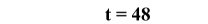
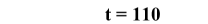
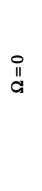
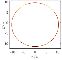
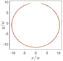
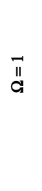
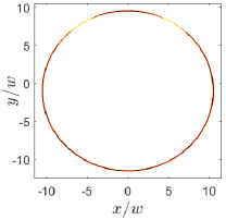
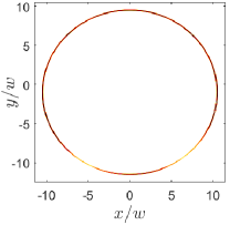
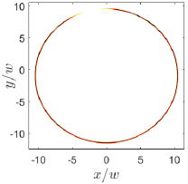
Figure B.1: Dynamics of the perturbative density modulations (lighter regions on the ring) for the non-rotating case (top panels) and rotating case with $\Omega=+1$ (bottom panels). From left to right $t=16,48$ and $110$. In the non-rotating case the modulations move with same speed in the ring and meet at the tunneling point where they were produced. For the rotating case, the modulation which moves counterclockwise is faster. It passes tunneling point and reaches the slower modulation on the left side of the tunneling point before the slow one can reach the tunneling region. Here only the tip of the atomic density with value between $0.0212$ to $0.022$ ($0.022$ being the maximum of density) are plotted. The white area has density lower than $0.0212$. Perturbations are around $3\%-4\%$ of the maximum density.

The exact value of $v_{0}$ and therefore $T_{0}$ and $T^{\pm}$ depend on the details of the excitations and the sound velocity in the system and we are not able to calculate them exactly for our system. However, having an estimation of the $T_{0}$ makes it possible to calculate $T^{\pm}$ and have an estimation of time delay between the fast and slow moving perturbations. In Fig. 2 of the main text, for the case with $\Omega=0$, the time when the first large dip in $N_{tot}$ takes place is an approximate value of $T_{0}$. In our system this time is $T_{0}=116$. Table 2 summarizes the analytical prediction of $T^{\pm}$, based on Bogoliubov calculations and numerical estimation of $T_{0}$, as well as numerical values extracted from Fig. 2 of the main text.

	Analytical		Numerical
$\Omega$	$T^{+}$	$T^{-}$	$T^{+}$	$T^{-}$
$\pm 1$	$112.193$	$120.075$	———	———
$\pm 2$	$108.628$	$124.446$	$110$	$125$
$\pm 3$	$105.282$	$129.147$	$108$	$129$

Table 2: The analytical estimation of $T^{\pm}$, based on Bogoliubov calculations and numerical estimation of $T_{0}$, compared with the values estimated from numerical results plotted in Fig. 2 of the main text.

In conclusion, the one-dimensional calculations based on Bogoliubov excitations together with our rough estimation of the value of $T_{0}$, predict a time delay of $15.818$ and $23.865$, for cases with $\Omega=\pm 2$ and $\Omega=\pm 3$ respectively, between the first arrival of the slow and fast density perturbations at the tunneling point. Our numerical data show delays of $15$ and $21$ respectively. The predicted values of $T^{\pm}$ for the case with $\Omega=\pm 1$ have not been resolved in our numerical data, due to the finite length of the density perturbations and limited time resolution of our saved data. However, the minimum in $N_{tot}$ for this case takes place around $t=115$ which is still earlier than $T_{0}$ and moreover the dip is much shallower and slightly wider than the non-rotating case. We attribute the discrepancy between the analytical and the (estimated) numerical $T_{0}$ to the finite residing time (time in which the suppression of the density stays localized, before the pair excitations start) that we observe to characterize the decay of the excitations.

References

- Leggett (1991) A. Leggett, in Granular Nanoelectronics (NATO ASI Ser. B, 251 Plenum, New York, 1991) p. 297.
- Seaman et al. (2007) B. T. Seaman, M. Krämer, D. Z. Anderson, and M. J. Holland, Phys. Rev. A 75, 023615 (2007).
- Amico et al. (2005) L. Amico, A. Osterloh, and F. Cataliotti, Phys. Rev. Lett. 95, 063201 (2005).
- Amico et al. (2017) L. Amico, G. Birkl, M. Boshier, and L.-C. Kwek, New J. Phys. 19, 020201 (2017).
- Barrett et al. (2014) B. Barrett, R. Geiger, I. Dutta, M. Meunier, B. Canuel, A. Gauguet, P. Bouyer, and A. Landragin, Comptes Rendus Physique 15, 875 (2014).
- Arnold et al. (2006) A. S. Arnold, C. S. Garvie, and E. Riis, Phys. Rev. A 73, 041606(R) (2006).
- Navez et al. (2016) P. Navez, S. Pandey, H. Mas, K. Poulios, T. Fernholz, and W. von Klitzing, New J. Phys. 18, 075014 (2016).
- Dumke et al. (2016) R. Dumke, Z. Lu, J. Close, N. Robins, A. Weis, M. Mukherjee, G. Birkl, C. Hufnagel, L. Amico, M. G. Boshier, et al., Journal of Optics 18, 093001 (2016).
- Dalibard et al. (2011) J. Dalibard, F. Gerbier, G. Juzeliūnas, and P. Öhberg, Rev. Mod. Phys. 83, 1523 (2011).
- Wright et al. (2013) K. C. Wright, R. B. Blakestad, C. J. Lobb, W. D. Phillips, and G. K. Campbell, Phys. Rev. Lett. 110, 025302 (2013).
- Ramanathan et al. (2011) A. Ramanathan, K. C. Wright, S. R. Muniz, M. Zelan, W. T. Hill, C. J. Lobb, K. Helmerson, W. D. Phillips, and G. K. Campbell, Phys. Rev. Lett. 106, 130401 (2011).
- Ryu et al. (2013) C. Ryu, P. W. Blackburn, A. A. Blinova, and M. G. Boshier, Phys. Rev. Lett. 111, 205301 (2013).
- Eckel et al. (2014) S. Eckel, J. G. Lee, F. Jendrzejewski, N. Murray, C. W. Clark, C. J. Lobb, W. D. Phillips, M. Edwards, and G. K. Campbell, Nature 506, 200 (2014).
- Yakimenko et al. (2015) A. I. Yakimenko, Y. M. Bidasyuk, M. Weyrauch, Y. I. Kuriatnikov, and S. I. Vilchinskii, Phys. Rev. A 91, 033607 (2015).
- Hallwood et al. (2006) D. W. Hallwood, K. Burnett, and J. Dunningham, New J. Phys. 8, 180 (2006).
- Solenov and Mozyrsky (2010) D. Solenov and D. Mozyrsky, Phys. Rev. Lett. 104, 150405 (2010).
- Amico et al. (2014) L. Amico, D. Aghamalyan, F. Auksztol, H. Crepaz, R. Dumke, and L. C. Kwek, Sci. Rep. 4 (2014).
- Aghamalyan et al. (2015) D. Aghamalyan, M. Cominotti, M. Rizzi, D. Rossini, F. Hekking, A. Minguzzi, L. C. Kwek, and L. Amico, New J. Phys. 17, 045023 (2015).
- Aghamalyan et al. (2016) D. Aghamalyan, N. Nguyen, F. Auksztol, K. Gan, M. M. Valado, P. Condylis, L. Kwek, R. Dumke, and L. Amico, New J. Phys. 18, 075013 (2016).
- Aghamalyan et al. (2013) D. Aghamalyan, L. Amico, and L. C. Kwek, Phys. Rev. A 88, 063627 (2013).
- Mathey and Mathey (2016) A. C. Mathey and L. Mathey, New J. Phys. 18, 055016 (2016).
- Haug et al. (2018) T. Haug, J. Tan, M. Theng, R. Dumke, L.-C. Kwek, and L. Amico, Phys. Rev. A 97, 013633 (2018).
- Zupancic et al. (2016) P. Zupancic, P. M. Preiss, R. Ma, A. Lukin, M. E. Tai, M. Rispoli, R. Islam, and M. Greiner, Opt. Express 24, 13881 (2016).
- Haase et al. (2017) T. Haase, D. White, D. Brown, I. Herrera, and M. Hoogerland, Rev. Sci. Instrum 88, 113102 (2017).
- Gauthier et al. (2016) G. Gauthier, I. Lenton, N. M. Parry, M. Baker, M. J. Davis, H. Rubinsztein-Dunlop, and T. W. Neely, Optica 3, 1136 (2016).
- Liang et al. (2009) J. Liang, J. Rudolph N. Kohn, M. F. Becker, and D. J. Heinzen, Appl. Opt. 48, 1955 (2009).
- Muldoon et al. (2012) C. Muldoon, L. Brandt, J. Dong, D. Stuart, E. Brainis, M. Himsworth, and A. Kuhn, New J. Phys. 14, 073051 (2012).
- Henderson et al. (2009) K. Henderson, C. Ryu, C. MacCormick, and M. G. Boshier, New J. Phys. 11, 043030 (2009).
- Jüngel and Mennemann (2010) A. Jüngel and J.-F. Mennemann, Mathematics and Computers in Simulation 81, 883 (2010).
- Antoine et al. (2013) X. Antoine, W. Bao, and C. Besse, Comput. Phys. Commun 184, 2621 (2013).
- (31) Appendix
- Kumar et al. (2016) A. Kumar, N. Anderson, W. D. Phillips, S. Eckel, G. K. Campbell, and S. Stringari, New J. Phys. 18, 025001 (2016).
- Anderson et al. (1994) R. Anderson, H. Bilger, and G. E. Stedman, Am. J. Phys 62, 975 (1994).
- (34) D. S. Petrov and G. V. Shlyapnikov, Phys. Rev. A 64, 012706 (2001).
- Beliaev (1958) S. Beliaev, Sov. Phys. JETP 34, 299 (1958).
- Giorgini (1998) S. Giorgini, Phys. Rev. A 57, 2949 (1998).
- Tan et al. (2010) S. Tan, M. Pustilnik, and L. I. Glazman, Phys. Rev. Lett. 105, 090404 (2010).
- Ristivojevic and Matveev (2016) Zoran Ristivojevic and K. A. Matveev, Phys. Rev. B 94, 024506 (2016).
- Ozeri et al. (2005) R. Ozeri, N. Katz, J. Steinhauer, and N. Davidson, Rev. Mod. Phys. 77, 187 (2005).
- Kivshar and Malomed (1989) Y. S. Kivshar and B. A. Malomed, Rev. Mod. Phys. 61, 763 (1989).
- Nguyen et al. (2014) J. H. Nguyen, P. Dyke, D. Luo, B. A. Malomed, and R. G. Hulet, Nature Physics 10, 918 (2014).
- Bao and Wang (2006) W. Bao and H. Wang, J. Comput. Phys 217, 612 (2006).