Frequency domain integrals for
stability preservation in Galerkin-type
projection-based model order reduction
Roland Pulch
Institute of Mathematics and Computer Science,
University of Greifswald,
Walther-Rathenau-Str. 47, 17489 Greifswald, Germany.
Email: roland.pulch@uni-greifswald.de
Abstract
|
We investigate linear dynamical systems consisting of
ordinary differential equations with high dimensionality.
Model order reduction yields alternative systems of much lower dimensions.
However, a reduced system may be unstable, although
the original system is asymptotically stable.
We consider projection-based model order reduction of Galerkin-type.
A transformation of the original system ensures that any reduced system
is asymptotically stable.
This transformation requires the solution of a high-dimensional
Lyapunov inequality.
We solve this problem using a specific Lyapunov equation.
Its solution can be represented as a matrix-valued integral
in the frequency domain.
Consequently, quadrature rules yield numerical approximations,
where large sparse linear systems of algebraic equations
have to be solved.
We analyse this approach and show a sufficient condition on the error
to meet the Lyapunov inequality.
Furthermore, this technique is extended to systems
of differential-algebraic equations with strictly proper transfer
functions by a regularisation.
Finally, we present results of numerical computations for
high-dimensional examples, which indicate the efficiency of
this stability-preserving method.
Keywords: linear dynamical system, ordinary differential equation, differential algebraic equation, model order reduction, Galerkin projection, asymptotic stability, Lyapunov equation, Lyapunov inequality, quadrature rule, frequency domain. MSC (2010): 65L05, 65L20, 34C20, 34D20, 93D20 |
1 Introduction
Numerical simulation represents a main tool for the investigation of dynamical systems in science, engineering and other fields of application. High-fidelity modelling is required to obtain detailed information on complex problems. However, the high-fidelity systems may have a huge number of state variables, which makes a numerical simulation expensive or even infeasible. Hence methods of model order reduction (MOR) are applied to decrease the dimensionality of the dynamical systems, see [2, 5, 34]. Yet the reduced system has to reproduce the quantities of interest sufficiently accurate.
We consider linear systems of ordinary differential equations (ODEs), which are asymptotically stable. Projection-based MOR determines linear ODEs with a lower dimensionality. However, the reduced system may be unstable and thus useless. Some solutions become unbounded for unstable systems in the time domain. Furthermore, error bounds, which follow from the transfer functions in the frequency domain, are not available any more. Hence stability-preserving MOR methods are essential to generate appropriate reduced systems.
The balanced truncation technique, see [15], always produces stable reduced systems, while the computational effort is often relatively large. Krylov subspace techniques, see [13], are less expensive, whereas stability can easily be lost. A stability preservation of a Krylov subspace approach is achieved by special assumptions and methods in [18]. A post-processing, which works on the poles of the transfer function, can recondition the stability, see [3].
We employ projection-based MOR of Galerkin-type, where each scheme is defined by a single orthogonal projection matrix. Important methods are the one-sided Arnoldi algorithm and the proper orthogonal decomposition (POD), for example. A transformation of the system of ODEs guarantees the stability of any reduced system, see [10, 29, 32]. This technique was also applied to a stochastic Galerkin projection in [31], where the stability of larger systems than the original ODEs is ensured. In our MOR methods, the main effort consists in solving a single high-dimensional Lyapunov inequality, where the efficient numerical solution is critical.
The Lyapunov inequality can be satisfied by the approximate solution of a high-dimensional Lyapunov equation. Therein, we perform a simple but effective choice of an input matrix. We prove an error bound on the approximation, which is sufficient for achieving the Lyapunov inequality. The solution of the Lyapunov equation also represents a matrix-valued integral in the frequency domain. Phillips and Silveira [28] computed integrals of this type approximately by a quadrature rule. Quadrature methods were also considered for such integrals in [6, 9]. We use this approach to construct a stability-preserving MOR technique. Therein, not the solution of the Lyapunov equation itself is required but an associated matrix-matrix product with a small number of columns. Now large sparse linear systems of algebraic equations have to be solved, where the linear dynamical system yields the coefficient matrices.
Furthermore, we extend this stability-preserving MOR method to systems of differential-algebraic equations (DAEs). Müller [26] investigated a regularisation technique, which changes an asymptotically stable DAE system into an asymptotically stable ODE system. Now the stability-preserving MOR applies to this system of ODEs. In the case of DAEs with a strictly proper transfer function, we show that the additional regularisation error converges to zero in dependence on a regularisation parameter.
The paper is organised as follows. We introduce the considered MOR methods in Section 2. The stability-preserving transformation and the Lyapunov equations are discussed in Section 3. We arrange the frequency domain integrals and analyse the usage of quadrature rules. In Section 4, the stability-preserving approach is transferred to systems of DAEs. Finally, we present results of numerical experiments in Section 5, where an ODE system and a DAE system are examined.
2 Model order reduction and stability
Projection-based MOR of linear dynamical systems is closely related to stability properties, which are reviewed in this section.
2.1 Linear dynamical systems and stability
We consider linear time-invariant systems in the form
| (1) |
with state/inner variables , inputs and outputs . The system includes constant matrices , and . If the mass matrix is non-singular, then the system (1) consists of ordinary differential equations (ODEs). If the mass matrix is singular, then differential-algebraic equations (DAEs) are given. The pair is called a matrix pencil. We assume that the matrix pencil is regular, i.e., for some . ODEs always yield a regular matrix pencil. We add predetermined initial values , which are assumed to be consistent in the case of DAEs.
In the frequency domain, a transfer function describes the input-output behaviour of the system (1) completely, see [2]. This transfer function reads as
| (2) |
The mapping (2) is a rational function with a finite set of poles . The magnitude of a transfer function can be characterised by norms in Hardy spaces. The -norm is defined by, see [36, p. 92],
| (3) |
with and the Frobenius (matrix) norm provided that the integral exists.
The stability issues of the system (1) are independent of the definition of inputs or outputs. To discuss the stability, we recall some general properties of matrices in the following definitions.
Definition 1
Let and be its eigenvalues. The spectral abscissa of the matrix is the real number
Definition 2
A matrix pencil is called stable, if and only if each eigenvalue characterised by has a strictly negative real part.
Definition 3
The linear dynamical system (1) is asymptotically stable if and only if its associated matrix pencil is stable.
In the case of a non-singular mass matrix, asymptotic stability of a system (1) is equivalent to the property of the spectral abscissa in Definition 1. Concerning Definition 2, a regular matrix pencil exhibits a finite set of eigenvalues. Furthermore, Definition 3 of asymptotic stability can also be found in [8, p. 376]. The asymptotic stability guarantees the existence of the transfer function (2) on the imaginary axis. The -norm (3) is always finite for asymptotically stable ODEs, whereas this norm may not exist in the case of (stable) DAEs.
If the matrix pencil has eigenvalues with non-positive real part and a real part zero appears, then Lyapunov stability may still be satisfied. We consider this instance also as a loss of stability, because the advantageous asymptotic stability is not valid any more.
2.2 Projection-based model order reduction
We assume that the linear dynamical system (1) exhibits a huge dimensionality . Thus the involved matrices and are typically sparse. The purpose of MOR is to decrease the complexity. An alternative linear dynamical system
| (4) |
has to be constructed with state/inner variables and the matrices , , , where the dimension is much smaller than . Initial values are derived from the initial values . Nevertheless, the output of (4) should be a good approximation to the output of (1), i.e., for all relevant times. The system (4) is called the reduced-order model (ROM) of the full-order model (FOM) given by (1).
The linear dynamical system (4) has its own transfer function of the form (2). If both the original system (1) and the reduced system (4) are asymptotically stable, then error bounds are available in the case of and . It holds that, see [4, p. 496],
| (5) |
with the -norm
| (6) |
the -norm (3), the maximum (vector) norm and the Euclidean (vector) norm .
In projection-based MOR, see [2], each approach yields two projection matrices of full rank. We obtain the matrices of the ROM (4) by
| (7) |
The orthogonality and sometimes the biorthogonality are supposed with the identity matrix .
Often the projection matrices result from the determination of subspaces, i.e.,
On the one hand, the original state/inner variables are approximated within the space by . On the other hand, the residual
| (8) |
is kept small by the requirement and thus for all .
2.3 Galerkin-type methods
A Galerkin-type projection (7) is characterised by the property . Thus we have to determine just a suitable projection matrix . Examples of Galerkin-type MOR methods are:
-
•
one-sided Arnoldi method, see [13],
-
•
proper orthogonal decomposition (POD), see [2, p. 277],
-
•
multi-parameter moment matching as in [21],
-
•
iterative improvement for the case of many outputs as in [12],
-
•
and others.
Moment matching methods identify an approximation of the transfer function (2) in the frequency domain. The one-sided Arnoldi scheme represents a Galerkin-type moment matching method. Alternatively, the POD technique employs information on a solution for a particular input in the time domain.
We explain the one-sided Arnoldi method, because it is used for the numerical experiments in Section 5. An expansion point is chosen. The matrix
| (9) |
is arranged, which includes the matrices of the linear dynamical system (1). Let a single input () be given without loss of generality. We define the matrix and the vector . The Krylov subspaces belonging to the matrix and the vector read as
| (10) |
for . The Arnoldi algorithm computes an orthonormal basis of the subspace (10) by a specific orthogonalisation scheme. The basis is collected in a matrix . Hence it holds that by construction. The projection matrix becomes real-valued in the case of . Otherwise, the projection matrix is obtained from a reorthogonalisation of the matrix . This technique can be generalised straightforward to the case of several expansion points and multiple inputs.
The computational effort of the one-sided Arnoldi method consists in two parts. Firstly, we compute an -decomposition of the high-dimensional matrix (9). The sparsity of the matrices often allows for an efficient computation. Each matrix-vector multiplication with some requires a solution of a linear system with coefficient matrix (9). Thus forward and backward substitutions are performed to determine (10). Secondly, basic linear algebra operations yield the orthonormal basis similar to the Gram-Schmidt orthogonalisation.
3 Stability preservation
We investigate linear dynamical systems (1) consisting of ODEs in this section.
3.1 Stability and Lyapunov equations
We consider the Lyapunov inequality
| (11) |
with from the dynamical system (1) and a (non-unique) solution . This problem consists in finding a symmetric positive definite matrix such that the left-hand side of (11) is negative definite. We can solve the problem by choosing any symmetric positive definite matrix . It follows that the generalised Lyapunov equation, cf. [27],
| (12) |
yields a unique symmetric positive definite solution , because the spectral abscissa from Definition 1 exhibits . This solution also satisfies the Lyapunov inequality (11).
Direct methods of linear algebra compute the solution of (12) or its Cholesky factorisation, see [17, 27]. However, direct methods are excluded in our context, since their computational effort is . Approximate methods are available like projection methods and the alternating direction implicit (ADI) iteration, see [19, 20, 40], for example. These methods often produce approximations with a low-rank factor (). Thus the approximation becomes a singular matrix, which makes the transformation dubious. Ill-conditioned reduced matrices arise sometimes as shown in [32].
Using the solution of the Lyapunov equation (12), we transform the ODEs (1) into the equivalent system
| (13) |
This transformation operates only in the image space and not in the state space. Stability preservation is given in a Galerkin-type MOR of the equivalent system (13). We cite a theorem, whose proof can be found in [32], for example.
Theorem 1
Let with be any projection matrix constructed for a reduction of the FOM (1). The Galerkin-type MOR with is applied to the transformed system (13) now. The matrices of the associated ROM (4) can be written in the form (7) with the projection matrix
| (14) |
Consequently, this reduction represents a special case of a (non-Galerkin-type) MOR (7) for the original system (1). It holds that in general. Biorthogonality is achieved by the alternative projection matrix
| (15) |
The ROMs obtained from (14) and (15) are equivalent and thus the stability properties coincide. The matrix in (14) is defined by matrix-matrix products. On the one hand, the evaluation is cheap, because is typically sparse. On the other hand, the matrix is dense. We require an approximation of such that the product is computable with relatively low effort. The Galerkin-type MOR for the system (1) and the MOR for the system (13) are not equivalent, since the residual (8) is not invariant in the used transformations.
3.2 Frequency domain integrals
There are two analytical formulas for the solution of the generalised Lyapunov equations (12), see [2, p. 177]. It holds that
| (16) |
including the matrix exponential in the time domain. The asymptotic stability of (1) implies and thus this matrix-valued integral exists. Alternatively, Parseval’s theorem induces the matrix-valued integral
| (17) |
in the frequency domain. The asymptotic stability of (1) yields the invertibility of the involved matrices. Although the integrand is complex-valued, the integral becomes real-valued.
Our idea is to apply the elementary choice with the identity matrix in the Lyapunov equation (12). The identity matrix features the maximum rank . Furthermore, there is no potential for a low-rank approximation of , because all eigenvalues are identical to one. A symmetry of the integrand allows for a restriction of the integration to non-negative frequencies. The frequency domain integral (17) simplifies to
| (18) |
using the abbreviation
| (19) |
In (16), the matrix exponential yield dense matrices. In (17), the matrices for are often sparse, whereas the inverse matrices are always dense. Hence we never compute the inverse matrices explicitly. Nevertheless, sophisticated algorithms often produce a sparse -decomposition of a matrix .
In an MOR with projection matrix (14), we require just the matrix-matrix product with the constant matrix . It follows that
| (20) |
which represents a matrix-valued integral of size in the frequency domain.
We do not use the formulation (16) in the time domain, because there is no suitable method to calculate the matrix exponential, see [24]. Appropriate iterative techniques to compute a matrix-vector product with the matrix exponential do exist, see [1]. However, rough approximations would confuse the error estimation of an adaptive quadrature method.
3.3 Error condition for Lyapunov inequality
We show the following general result to characterise the influence of errors in the context of the Lyapunov inequality (11).
Theorem 2
Proof:
It holds that
with a symmetric matrix . Subtraction yields
Let . We estimate
Now the condition (21) is sufficient for and thus .
Let and for be the eigenvalues of and , respectively. It follows that
We obtain for all . Consequently, the matrix is positive definite and the matrix is negative definite. Since represents the solution of a Lyapunov equation (12) including the symmetric positive definite matrix , inherits the positive definiteness.
If we employ the spectral (matrix) norm, then the above constant simplifies to . However, the evaluation of the spectral norm takes more effort in comparison to the norms .
An obvious question is if a sufficient condition can be derived for the relative error . However, we require an upper bound on in this case, which becomes more involved. In [38, p. 100], the analysis yields the estimate
including the inverse of the Lyapunov operator in the Frobenius norm. Yet this upper bound cannot be simplified in the case of general matrices and .
We obtain a necessary condition on the relative error with respect to the requirement (21).
Lemma 1
Proof:
3.4 Quadrature methods
Phillips and Silveira [28] investigated the integrals (17) including with a low-rank factor (). Therein, a quadrature method with nodes and positive weights yields an approximation with a factor . Hence both the rank and the number of nodes has to be small. This requirement disappears in our approach using .
We also apply a quadrature rule to our frequency domain integrals. For theoretical investigations, we define an approximation of (18) by
| (23) |
with nodes and weights for . The quadrature introduces an error. Nevertheless, the approximations (23) always own the following desired properties independent of the magnitude of the error.
Lemma 2
If the quadrature rule involves positive weights only, then the approximation in (23) is always symmetric and positive definite.
Proof:
We define with real-valued matrices . It follows that
Now the symmetry of is obvious. We show the definiteness. Let . We obtain
It holds that or for each , because otherwise would cause a contradiction to the non-singularity of the matrix . It follows that the above sum is strictly positive.
The associated approximation of (20) reads as
| (24) |
It turned out that this approach is similar to a quadrature technique given in [6], where an integral of the form (17) yields the Gramian of a linear dynamical system with many outputs.
Lemma 2 shows that the matrix is always symmetric and positive definite in (24). Consequently, the underlying transformation is non-singular, which represents a crucial advantage in comparison to methods for Lyapunov equations (12) producing low-rank approximations. Theorem 2 implies that an approximation satisfying (21) guarantees a stability preservation in an MOR. However, the approximation errors cannot be checked in practise, because the exact solution is unknown. We compute an approximation (24), where an adaptive quadrature yields errors below predetermined tolerances. Yet there is no direct connection to the errors in the counterpart (23).
3.5 Numerical solution of linear systems
Our aim is to evaluate the approximation (24) without computations of matrices of size . Thus we solve complex-valued linear systems
| (25) |
for each with the matrices (19), a predetermined matrix and the unknowns . We consider only direct approaches of numerical linear algebra. Iterative methods introduce an additional error, which restricts the accuracy of high-order quadrature rules. Our aim is to use as less nodes as possible.
There are two possibilities to solve a linear system (25) directly now:
-
(i)
The matrix-matrix product is computed. An algorithm for sparse matrices generates a Cholesky-decomposition . We determine the solution by forward and backward substitutions for multiple right-hand sides.
-
(ii)
An -decomposition including pivoting with row as well as column reordering is applied to the matrices (19), i.e.,
(26) with orthogonal permutation matrices . It follows that
represents an -decomposition of . We obtain
using permutations, forward and backward substitutions for multiple right-hand sides.
We do not apply the approach (i) in our numerical computations for two reasons: (i) The matrix is less sparse than a matrix (19). Thus a Cholesky factorisation of may not be (significantly) faster than an -decomposition of . (ii) The condition number increases considerably due to with respect to the spectral norm.
3.6 Integrals on finite intervals
Concerning the integrals (20), we can straightforward transform the infinite frequency domain to the finite interval . The substitution or, equivalently, yields
| (27) |
An advantage is that the evaluation of the integrand at exists in the limit
| (28) |
provided that the mass matrix is non-singular. Now any (open or closed) quadrature rule for finite intervals generates an approximation to the integral (27). Numerical tests indicate that the Gauss-Legendre quadrature is superior for computing the integral (27) in comparison to other common schemes. The reason is that the integrand is analytic in the open interval .
An adaptive Gauss-Kronrod quadrature rule was considered for integrals of this type in [6]. However, as mentioned in Section 3.4, the quadrature is not required to be sufficiently accurate for the integrals (27) but the inherent integrals (18). An alternative is to use an adaptive refinement of nested quadrature rules until a desired set of ROMs becomes asymptotically stable. Note that it is cheap to check the stability for low-dimensional systems.
An elementary adaptive method of this type can be based on the midpoint rule. The nodes read as for with step size . The iteration for induces a sequence of nested grids, where the evaluations of the integrand in (27) can be reused. The iteration is terminated if all considered ROMs become stable.
4 Application to differential-algebraic equations
The technique of Section 3 cannot be applied directly to systems of DAEs (1). A singular mass matrix implies for and any . Hence the Lyapunov equation (12) is not fulfilled for each definite matrix . The associated integral (17) does not exist, even though the integrand is always well-defined in the case of a stable matrix pencil with respect to Definition 2. Likewise, the limit (28) does not exist.
4.1 Kronecker normal form
A linear dynamical system (1) with a singular mass matrix can be transformed into the Kronecker normal form, see [16, p. 452]. There are non-singular matrices such that
| (29) |
with a matrix and a nilpotent strictly upper triangular matrix (). The system (1) splits into a slow and a fast subsystem
| (30) |
with and . The input terms are omitted in (30), because they do not influence the stability properties of the systems. The smallest integer such that and is called the nilpotency index of the DAE system.
4.2 Regularisation
In [23], a system of DAEs was regularised straightforward under the assumption of semi-explicit systems. Alternatively, we apply an approach for general descriptor systems from [26], which goes back to [39]. The matrix pencil is modified into by
| (31) |
with parameters . The matrix is non-singular for all , because otherwise some would be an eigenvalue of the stable matrix pencil . The theorem below follows from the results in [26].
Theorem 3
The upper bound (32) is unknown in general, because the Kronecker normal form (29) is not available in practise. Nevertheless, Theorem 3 tells us that a regularisation to a stable system is feasible for all sufficiently small . Furthermore, the sparsity pattern of is identical to the sparsity pattern of . Thus the computational effort for a solution of linear systems does not change significantly.
4.3 Error estimates
We reduce the regularised system with matrices (31) instead of the original descriptor system (1). This approach is appropriate, if error bounds can be provided for the transfer functions. It holds that
| (33) |
in each norm, where and are the transfer functions of the regularised system and its ROM, respectively. The difference depends on the quality of the MOR. We discuss the difference in the following.
A linear dynamical system (or its transfer function) is called strictly proper, if and only if the transfer function satisfies
A system of ODEs always exhibits a strictly proper transfer function. The transfer function of a general system of DAEs reads as, see [7],
| (34) |
with a strictly proper part and a polynomial part . The polynomial part either vanishes or represents a non-zero matrix-valued polynomial of degree at most with the index of the system. These properties also depend on the definition of inputs and outputs in each system.
If the polynomial part vanishes, then the -norm (3) as well as the -norm of the transfer function (34) exist independent of the index. The -norm is always finite in the case of index-one systems. In [14], for example, the electric circuit of the Miller integrator is modelled by a linear DAE system of index , where the polynomial part becomes zero for the transfer function relating the input voltage to the output voltage.
We provide an error bound for the regularisation on compact frequency intervals, which is relevant in this context.
Lemma 3
Assume that the DAE is asymptotically stable and the ODE is given by (31) with . For each there are constants such that
| (35) |
uniformly for all frequencies provided that , where the spectral (matrix) norm is used.
Proof:
Let , and in this proof. We assume a bound on due to (32). Theorem 3 implies that the ODE is asymptotically stable. Thus the transfer functions exist and are continuous on the imaginary axis. The spectral norm is submultiplicative for matrices of any size. Thus we estimate
We use the abbreviations and . A general estimate on the difference between inverse matrices is available in a subordinate matrix norm. It follows that
provided that . On the one hand, the definition (31) with and implies
for all with the constant . On the other hand, we require the constant
such that for all . We obtain
for all provided that . Consequently, the constants read as and .
Lemma 3 demonstrates that error of the regularisation is low on a compact frequency domain for sufficiently small parameters . An error estimate of the type (35) cannot be derived uniformly for all , because the integral (17) does not exist in the limit . Thus high frequencies represent the critical part. If a system of DAEs (1) has a strictly proper transfer function, then this problem becomes obsolete.
Theorem 4
Proof:
The restriction , see (32), for some (close to the upper bound) and ensures the existence of each -norm. The -norm of the difference reads as
including the Frobenius (matrix) norm. Let . The assumptions imply that each component of is a rational function of , where the degree of the numerator is less than the degree of the denominator. The coefficients of the rational functions depend continuously on the parameters .
We discuss the part for high frequencies, i.e.,
with . It follows that
for each and , where the convergence is monotone from above (for ). The parameter interval is compact. Dini’s theorem yields
Hence we obtain a frequency such that
The integration domain exhibits the same bound due to a symmetry.
Now we apply Lemma 3 to the interval and obtain a bound (35) with constants . Let . The matrix norms exhibit the general bound . We obtain
provided that with the constant
Thus the estimate (36) is satisfied for all with the single constant and .
Theorem 4 illustrates that a regularisation with a low error in the -norm can be achieved provided that the parameters are chosen sufficiently small. The derived constants are pessimistic, because rough estimates appear in the proof. The magnitude of appropriate regularisation parameters depends on the system of DAEs (1). However, tiny parameters cause problems in numerical computations due to ill-conditioned matrices, for example.
If the system of DAEs is just proper, then the polynomial part in (34) represents a (non-zero) constant. Consequently, both the -error and the -error of the regularisation do not become arbitrarily small. There is still some potential for using this regularisation technique. The input-output relation of the linear dynamical system (1) is given by with the Laplace transforms of input and output, respectively. If a particular input induces a Laplace transform with a sufficiently fast decay for high frequencies, then the same effect as in a strictly proper system emerges.
5 Numerical experiments
We apply the stability-preserving technique from Section 3 to two high-dimensional examples now. All numerical computations were executed by the software package MATLAB [22].
5.1 Microthruster benchmark
In [25], a microthruster unit represents a test example called boundary condition independent thermal model. A spatial discretisation of the two-dimensional heat transfer partial differential equation yields a system of ODEs. More details can be found in [33]. Three parameters appear in this model, which we choose all equal to one. The linear dynamical system (1) is single-input-multiple-output (SIMO) with . Its Bode plot is depicted in Figure 1. Table 1 illustrates some properties of the system. In particular, the system is asymptotically stable. The matrix is diagonal with positive elements. Thus we simply scale this system into explicit ODEs (), which are used in the following.
| dimension | 4257 |
| # outputs | 7 |
| # non-zero entries in | 37465 |
| # non-zero entries in | 4257 |
| spectral abscissa |
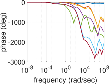
We use the one-sided Arnoldi method with the single real expansion point . The reduced systems are arranged for . The spectral abscissas of the reduced systems are depicted in Figure 2. It follows that 11 ROMs become unstable, which are all in the range . Thus we apply the stability preserving approach from Section 3.
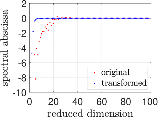
A quadrature method requires the solution of linear systems (25). We investigate the sparsity in the -decomposition (26) of the matrix (). The number of non-zeros in the -decomposition with partial pivoting () is . Alternatively, UMFPACK achieves a factorisation with non-zero entries, whose sparsity pattern is shown in Figure 3 (right).
We investigate three quadrature methods for the computation of the projection matrix (24):
-
i)
adaptive Gauss-7-Kronrod-15 quadrature using the built-in MATLAB function integral, see [35],
-
ii)
Gauss-Legendre rule, see [37, p. 171], with fixed numbers of nodes,
-
iii)
nested midpoint rules as described in Section 3.6.
In the adaptive quadrature (i), we choose the absolute and the relative error tolerances as . The algorithm performs evaluations of the integrand. The projection matrices (15) are used to attain biorthogonality. All reduced systems become stable now. Figure 2 depicts the spectral abscissas of the ROMs. In the Gauss-Legendre rule (ii), we increase the number of nodes until all ROMs become stable, see Table 2. Just nodes are sufficient to obtain always stable systems. Table 3 shows the number of stable ROMs for the refinement in the midpoint rule (iii). Now nodes are required to achieve the stability preservation in all reduced systems.
| # nodes | 1 | 2 | 4 | 5 | 6 | 7 | 9 | 11 | 14 |
| # stable systems | 91 | 92 | 93 | 94 | 96 | 97 | 98 | 99 | 100 |
| # nodes | 1 | 3 | 7 | 15 | 31 | 63 | 127 |
|---|---|---|---|---|---|---|---|
| # stable systems | 91 | 93 | 93 | 95 | 98 | 99 | 100 |
We also compare the approximation quality between the ROMs obtained from the conventional reduction and the stabilisation method. Figure 4 illustrates the relative error in the -norm (3), i.e.,
| (37) |
including the transfer functions. We calculate approximations of -norms (3) by the trapezoidal rule on a logarithmically spaced grid on the imaginary axis. The ROMs from the adaptive Gauss-Kronrod rule () and the Gauss-Legendre rule () are examined. We observe that the error (37) of the stabilisation method is often much lower than the conventional method for dimensions , whereas the errors become close for . Furthermore, the adaptive quadrature is more accurate than the Gauss-Legendre rule with the low number of nodes for . Our important observation is that the stabilisation approach does not deteriorate the accuracy of the MOR.
5.2 Random low-pass filter
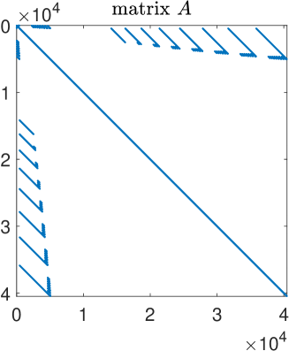
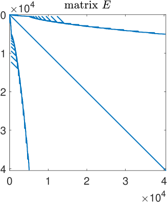
We investigate the electric circuit of a low-pass filter in Figure 5. The circuit includes 21 physical parameters: seven capacitances, six inductances and eight conductances. A mathematical modelling generates a system of DAEs (1) for 14 node voltages and 6 branch currents (). The (nilpotency) index of this system is one. Furthermore, the system is asymptotically stable and strictly proper. The system is single-input-single-output (SISO), because a voltage source is supplied and the output is defined as the voltage at a load conductance.

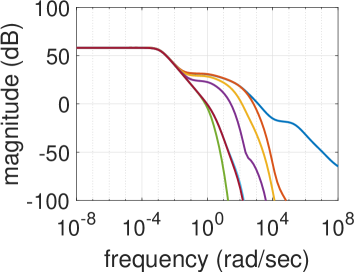
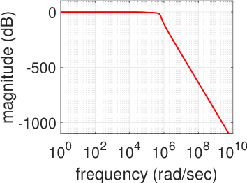
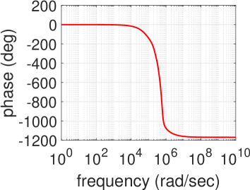
In a stochastic modelling, all physical parameters are replaced by uniformly distributed random variables with a variation of 15% around their mean values. We use a truncated polynomial chaos expansion to approximate the random processes, see [41]. All basis polynomials are included up to total degree three, i.e., basis functions depending on 21 variables. The stochastic Galerkin method yields a larger system of DAEs (1) with dimension , whose solution approximates the unknown coefficient functions. Table 4 depicts its characteristic numbers. The system is SIMO with a large number of outputs. This linear dynamical system inherits the properties of the circuit model: index-one, asymptotically stable and strictly proper. Figure 6 illustrates the Bode plot of the first output, which represents an approximation for the expected value of the output voltage. The magnitude of the transfer function shows that high frequencies are damped out. This test example was also used in [30].
| dimension | 40480 |
|---|---|
| # outputs | 2024 |
| # non-zero entries in | 116886 |
| # non-zero entries in | 32890 |
| rank() | 26312 |
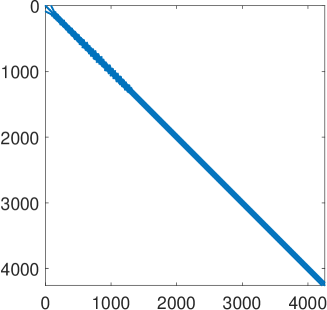
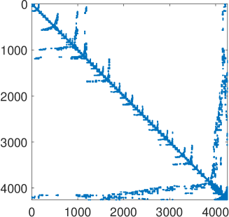
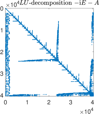
Furthermore, Figure 7 depicts the sparsity patterns of the system matrices and the -decomposition (26) for . UMFPACK yields an -factorisation with about million non-zero entries. In contrast, the common -factorisation with partial pivoting generates about 150 million non-zero elements and thus requires much more computational work. Consequently, we employ decompositions from UMFPACK whenever linear systems of this type appear.
Now the one-sided Arnoldi method with the single real expansion point is used in all cases. The ROMs are always computed for dimensions . We directly reduce the system of DAEs first. The relative -errors (37) of the MOR are depicted in Figure 8 (left). This error decays rapidly and becomes tiny. However, only 6 out of 100 ROMs inherit the asymptotic stability of the FOM. Hence a stability-preserving method is essential in this example.
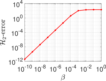
The system of DAEs is regularised by the technique described in Section 4.2. We arrange the modified matrices (31) with for different parameters . The total error (33) is bounded by the sum of regularisation error and MOR error. Figure 8 (right) shows the (absolute) -error of the regularisation. We recognise that this error converges exponentially to zero for tending to zero. In addition, numerical computations confirm that the investigated regularised systems are asymptotically stable.
On the one hand, we apply the conventional Arnoldi method to the systems of ODEs for several parameters . On the other hand, we perform the stabilisation technique of Section 3 for the ODEs in combination with the Arnoldi algorithm. The adaptive Gauss-Kronrod quadrature yields the associated projection matrix as in Section 5.1. The used error tolerances read as again. Table 5 illustrates the number of stable ROMs and the number of nodes in the quadrature. The conventional approach generates more and more unstable systems for decreasing parameters . In contrast, the stabilised method always yields at least 95% stable reduced systems. Moreover, the unstable ROMs occur only within dimensions . The number of nodes, which are selected by the adaptive quadrature, increases for decaying parameters . This behaviour reflects that the integral (20) does not exist in the limit case . However, the ratios of the regularisation parameter and the number of nodes still converges nearly exponentially to zero in the observed range. Thus the rise in is much lower than the decay in . It turns out that alleviated tolerances cause more unstable systems. Furthermore, the Gauss-Legendre rule performs worse in this example.
| parameter | ||||||
|---|---|---|---|---|---|---|
| # stable, conventional | 100 | 77 | 56 | 57 | 51 | 43 |
| # stable, stabilised | 100 | 99 | 95 | 95 | 95 | 95 |
| # nodes in quadrature | 180 | 330 | 480 | 600 | 810 | 900 |
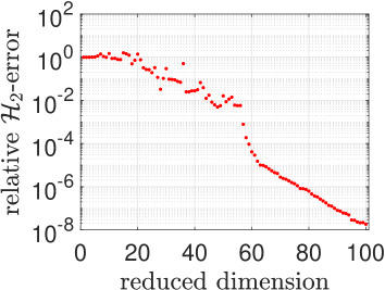
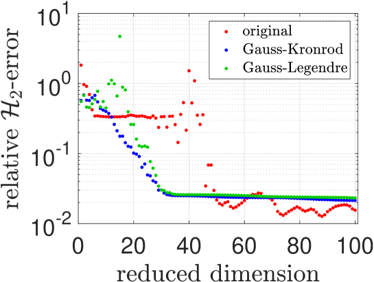
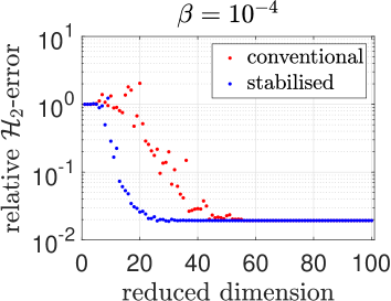
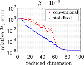
Finally, we examine the total error (33) of the MOR, where the system of DAEs represents the FOM. Figure 9 shows the relative errors with respect to the -norm in the two cases . The error decreases fastly for low reduced dimensions. Thereafter the total error stagnates, because the error of the regularisation dominates. We observe that the total error of the stability-preserving approach is always smaller or equal in comparison to the conventional technique. Moreover, the stabilised MOR method yields much smaller errors in the case of low dimensions.
6 Conclusions
In Galerkin-type projection-based MOR, stability preservation can be achieved by a transformation of a projection matrix. The transformation is associated with a high-dimensional Lyapunov inequality, which is satisfied by solving a specific Lyapunov equation. We designed a numerical method to compute the alternative projection matrix, where quadrature methods determine approximations of integrals in the frequency domain. In contrast to other numerical solvers of high-dimensional Lyapunov equations, our frequency domain integral ensures that the inherent approximate solution is a non-singular matrix. Results of numerical computations demonstrate that our approach is efficient in the case of ODEs.
We also generalised the numerical technique to DAEs by a regularisation. Again quadrature rules, which are applied to frequency domain integrals, yield the projection matrices for the regularised ODEs. However, the quadrature methods require more and more nodes for decreasing regularisation parameters, This property restricts the efficiency of our approach to some extend in the case of DAEs.
References
- [1] A.W. Al-Mohy, N.J. Higham, Computing the action of the matrix exponential with an application to exponential integrators, SIAM J. Sci. Comput. 33 (2011), 488–511.
- [2] A.C. Antoulas, Approximation of Large-Scale Dynamical Systems, SIAM Publications, 2005.
- [3] Z. Bai, R. Freund, A partial Padé-via-Lanczos method for reduced order modeling, Linear Algebra Appl. 332–334 (2001), 139–164.
- [4] P. Benner, S. Gugercin, K. Willcox, A survey of projection-based model order reduction methods for parametric dynamical systems, SIAM Review 57 (2015), 483–531.
- [5] P. Benner, V. Mehrmann, D.C. Sorensen, Dimension Reduction of Large-Scale Systems, Lecture Notes in Compuational Science and Engineering, Vol. 45, Springer, 2005.
- [6] P. Benner, A. Schneider, Balanced truncation model order reduction for LTI systems with many inputs or outputs, In: Proceedings 19th International Symposium on Mathematical Theory of Networks and Systems, 2010, pp. 1971–1974.
- [7] P. Benner, T. Stykel, Model order reduction of differential-algebraic equations: a survey, In: A. Ilchmann, T. Reis (eds.), Surveys in Differential-Algebraic Equations IV, Differential-Algebraic Equations Forum, Springer, 2017, pp. 107–160.
- [8] M. Braun, Differential Equations and Their Applications, 3rd ed., Springer, 1983.
- [9] T. Breiten, Structure-preserving model reduction for integro-differential equations, SIAM J. Control Optim. 54 (2016), 2992–3015.
- [10] R. Castañé Selga, B. Lohmann, R. Eid, Stability preservation in projection-based model order reduction of large scale systems, Eur. J. Control 18 (2012), 122–132.
- [11] T.A. Davis, UMFPACK User Guide, Technical Report, version 5.7.7, 2018.
- [12] F.D. Freitas, R. Pulch, J. Rommes, Fast and accurate model reduction for spectral methods in uncertainty quantification, Int. J. Uncertain. Quantif. 6 (2016), 271–286.
- [13] R. Freund, Model reduction methods based on Krylov subspaces, Acta Numerica 12 (2003), 267–319.
- [14] M. Günther, U. Feldmann, J. ter Maten, Modelling and discretization of circuit problems, in: P.G. Ciarlet (ed.), Handbook of Numerical Analysis, Vol. 13, Elsevier, 2005, pp. 523–659.
- [15] S. Gugercin, A.C. Antoulas, A survey of model reduction by balanced truncation and some new results, Int. J. Control 77 (2004), 748–766.
- [16] E. Hairer, G. Wanner, Solving Ordinary Differential Equations II: Stiff and Differential-Algebraic Problems, 2nd Ed., Springer, 1996.
- [17] S.J. Hammarling, Numerical solution of stable non-negative definite Lyapunov equation, IMA J. Numer. Anal. 2 (1982), 303–323.
- [18] T.C. Ionescu, A. Astolfi, On moment matching with preservation of passivity and stability, in: 49th IEEE Conference on Decision and Control, 2010, pp. 6189–6194.
- [19] B. Kramer, J.R. Singler, A POD projection method for large-scale algebraic Riccati equations, Numer. Algebra Contr. Optim. 6 (2016), 413–435.
- [20] J.-R. Li, J. White, Low rank solution of Lyapunov equations, SIAM J. Matrix Anal. & Appl. 24 (2002), 260–280.
- [21] P. Li, F. Liu, X. Li, L. Pileggi, S. Nassif, Modeling interconnect variability using efficient parametric model order reduction. In: Proc. of Design Automation and Test In Europe Conference (DATE) 2005, pp. 958–963.
- [22] MATLAB, version 9.4.0.813654 (R2018a), The Mathworks Inc., Natick, Massachusetts, 2018.
- [23] K. Mohaghegh, R. Pulch, J. ter Maten, Model order reduction using singularly perturbed systems, Appl. Numer. Math. 103 (2016), 72–87.
- [24] C. Moler, C. Van Loan, Nineteen dubious ways to compute the exponential of a matrix, twenty-five years later, SIAM Review 45 (2003), 3–49.
-
[25]
”MOR Wiki”, online document,
https://morwiki.mpi-magdeburg.mpg.de/morwiki Cited May 4, 2018. - [26] P.C. Müller, Modified Lyapunov equations for LTI descriptor systems, J. Braz. Soc. Mech. Sci. & Eng. 28 (2006), 448–452.
- [27] T. Penzl, Numerical solution of generalized Lyapunov equations, Adv. Comput. Math. 8 (1998), 33–48.
- [28] J. Phillips, L.M. Silveira, Poor man’s TBR: a simple model reduction scheme, IEEE Trans. Comput.-Aided Design Integr. Circuits Syst. 24 (2005), 43–55.
- [29] S. Prajna, POD model reduction with stability guarantee, in: Proceedings of 42nd IEEE Conference on Decision and Control, Maui, Hawaii, USA, December 2003, pp. 5254–5258.
- [30] R. Pulch, Model order reduction and low-dimensional representations for random linear dynamical systems, Math. Comput. Simulat. 144 (2018), 1–20.
- [31] R. Pulch, F. Augustin, Stability preservation in stochastic Galerkin projections of dynamical systems, arXiv:1708:00958 (2017).
-
[32]
R. Pulch,
Stability preservation in Galerkin-type projection-based model order reduction,
arXiv:1711:02912 (2017).
to appear in: Numerical Algebra, Control and Optimization (NACO) - [33] E.B. Rudnyi, J.G. Korvink, Boundary Condition Independent Thermal Model, In: P. Benner, V. Mehrmann, D.C. Sorensen (eds.), Dimension Reduction of Large-Scale Systems, Lecture Notes in Compuational Science and Engineering, Vol. 45, Springer, 2005, pp. 345–348.
- [34] W.H.A. Schilders, M.A. van der Vorst, J. Rommes (eds.), Model Order Reduction: Theory, Research Aspects and Applications, Mathematics in Industry, Vol. 13, Springer, 2008.
- [35] L.F. Shampine, Vectorized adaptive quadrature in MATLAB, J. Comput. Appl. Math. 211 (2008), 131–140.
- [36] Y. Shmaliy, Continuous-Time Systems, Springer, 2007.
- [37] J. Stoer, R. Bulirsch, Introduction to Numerical Analysis, 3rd ed., Springer, 2002.
- [38] T. Stykel, Analysis and Numerical Solution of Generalized Lyapunov Equations, PhD thesis, Technische Universität Berlin, 2002.
- [39] Q. Wang, Q.L. Zhang, G.S. Zhang, W.Q. Liu, Lyapunov equations with positive definite solution for descriptor systems, In: Proc. 4th Asian Control Conf. (ASCC), WA9-16, Singapore, 2002, pp. 385–389.
- [40] T. Wolf, H. Panzer, B. Lohmann, Model order reduction by approximate balanced truncation: a unifying framework, Automatisierungstechnik 61 (2013), 545–556.
- [41] D. Xiu, Numerical Methods for Stochastic Computations: a Spectral Method Approach, Princeton University Press, 2010.