AsySPA: An Exact Asynchronous Algorithm for Convex Optimization Over Digraphs
Abstract
This paper proposes a novel exact distributed asynchronous subgradient-push algorithm (AsySPA) to solve an additive cost optimization problem over directed graphs where each node only has access to a local convex function and updates asynchronously with an arbitrary rate. Specifically, each node of a strongly connected digraph does not wait for updates from other nodes but simply starts a new update within any bounded time interval by using local information available from its in-neighbors. “Exact” means that every node of the AsySPA can asymptotically converge to the same optimal solution, even under different update rates among nodes and bounded communication delays. To address uneven update rates, we design a simple mechanism to adaptively adjust stepsizes per update in each node, which is substantially different from the existing works. Then, we construct a delay-free augmented system to address asynchrony and delays, and study its convergence by proposing a generalized subgradient algorithm, which clearly has its own significance and helps us to explicitly evaluate the convergence rate of the AsySPA. Finally, we demonstrate advantages of the AsySPA in both theory and simulation.
Index Terms:
Distributed optimization, asynchronous algorithms, directed graphs, adaptive stepsize, Asynchronous subgradient-push algorithm (AsySPA).I Introduction
Our objective is to distributedly solve an additive cost optimization problem over a directed graph (digraph) where each summand is privately preserved by a computing node. This problem is usually referred to as the distributed optimization problem (DOP) and has attracted considerable attention in the past decade, see e.g. [1] and references therein.
To solve DOPs, there are two types of distributed algorithms: synchronous and asynchronous algorithms. The distinct feature between them is that nodes in asynchronous algorithms do not wait for updates from other nodes but simply compute updates using its currently available information. This allows them to complete updates much faster than the synchronous ones and eliminates the costly synchronization penalty, which is especially outstanding for the case with a large scale number of heterogeneous nodes [2]. However, asynchrony also brings many challenges in the design and analysis of effective algorithms. This paper proposes a novel exact asynchronous subgradient-push algorithm (AsySPA) to solve the DOP over digraphs.
I-A Synchronous versus asynchronous algorithms
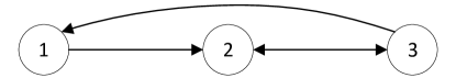
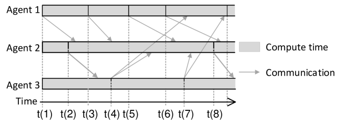
We use Fig. 2 to elaborate the striking differences between synchronous and asynchronous algorithms by taking the digraph in Fig. 1 as an example. In Fig. 2, the line with an arrow represents the communication direction between nodes, which also allows possible transmission delays. In a synchronous algorithm (see Fig. LABEL:sub@fig3a:exp2), all the nodes start to update at the same time where denotes the number of updates of the network and should be known to all nodes. In an asynchronous algorithm (see Fig. LABEL:sub@fig3b:exp2), each node computes update independently. Particularly, it can start a new update immediately after finishing the current one by possibly using multiple receptions from one neighbor.
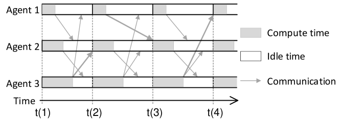
Obviously, all the nodes in a synchronous algorithm need to agree on the update time , which usually needs a global clock or synchronization of all nodes. It is worthy mentioning that the clock synchronization is not easy for a large-scale system and has been studied for quite a long time [3]. From this point of view, an asynchronous algorithm is much easier to implement. Since some nodes may compute updates much faster, it takes relatively long idle time to wait for the slowest node in a synchronous algorithm, which potentially reduces the computational efficiency. In fact, many numerical experiments indeed suggest better performance of asynchronous algorithms [4]. A more throughout discussion can be found in [5].
However, it is much more challenging to design an effective asynchronous algorithm. Usually, a good synchronous algorithm may become invalid if we naively implement it in an asynchronous fashion. For example, if there exists asynchrony in implementing the celebrated synchronous SPA (SynSPA) [6], each node can only converge to a neighborhood of an optimal solution, the size of which depends on the degree of asynchrony [7]. In contrast, each node of the AsySPA in this paper converges to the same optimal solution.
I-B Literature review
The study of synchronous algorithms for the DOP is relatively mature, see e.g. [8, 9, 10, 11, 12, 6, 13, 14, 15]. Note that many distributed algorithms under time-varying graphs (e.g. [6]) are synchronous as a global clock is still required. Recently, the interest is shift to the design of asynchronous algorithms [16, 17, 18, 19, 20, 21, 22, 23, 24, 25, 26, 27, 7, 28, 29, 30, 31]. To better distinguish asynchronous algorithms, let be the sequence of update times of node and define the update rate of node in the asymptotic sense, i.e.,
| (1) |
where returns the cardinality of a set and is total number of computing nodes. Clearly, is unknown for a generic asynchronous algorithm. The AsySPA of this work aims to simultaneously overcome the following difficulties.
-
(a)
Each node independently computes a new update without waiting for others by using its currently available information from its in-neighbor nodes. This can maximumly reduce the idle time of the node and fully exploit the computational resource. Obviously, this also easily results in Uneven Update Rates (UUR) among nodes, i.e., for some , and that none, one or multiple nodes can update their variables at any time.
- (b)
- (c)
Asynchronous algorithms can be categorized depending on whether they are dealing with UUR or Even Update Rates (EUR). In [16, 17, 18], the convergence of their algorithms is proved only under EUR. For example, the time interval between two consecutive updates in [16, 17] is an identically and independently distributed process among nodes, which obviously results in EUR. Although it is extended to UUR in [19], it requires an essential process called logic-AND for synchronization, which introduces the costly synchronization penalty and is not necessary for the AsySPA. The algorithm in [18] requires that all nodes are randomly activated with the same probability, which again results in EUR. Although the edge-based asynchronous algorithms in [20, 21] are valid with UUR, they require two nodes to concurrently compute updates, which easily results in deadlock. This is obviously very different from our case with UUR. Moreover, the aforementioned works [16, 17, 19, 18, 20, 21] are only applicable to undirected graphs and do not consider communication delays.
The algorithms in [22, 23, 24] are proposed to handle the UUR problem, but they require the update rate to design algorithms, which is impractical in real applications, see also [23, Remark 1] and [27]. For example, the major results of Theorems 3-4 in [23] depend on the statistics of the activation random variable of each node, which is equivalent to have access to the update rate.
The asynchronous setting of this work is mostly close to that in [26, 27, 7, 28]. As mentioned before, the algorithm in [7] is a naive extension of the SynSPA and is unable to converge to an optimal solution of the DOP under UUR. In [26], the asynchronous algorithm combines the Newton-Raphson method with the robust push-sum consensus. Then, its convergence depends on stepsizes and initial conditions, both of which should be carefully selected. Moreover, it only considers lossy broadcast communications rather than information delays. In [27], the ASY-SONATA is proposed by integrating ideas of the robust push-sum consensus and the SONATA [37], and its exact convergence is proved if each local objective function is strongly convex with Lipschitz continuous gradient. Since the gradient tracking is key to the ASY-SONATA, it is unclear whether it is applicable on non-smooth convex functions. Moreover, its implementation seems much more complicated than that of the AsySPA. In the seminal work [28], each node asynchronously updates a component of the decision vector, which is different from the DOP. This problem is also of high interest and keeps attracting attention [29, 30]. For example, it has been adopted for the DOP in [30]. However, it is unable to converge to an exact optimal solution of the DOP. The work [31] provides sufficient conditions for the convergence of a class of asynchronous stochastic distributed algorithms, which are related to contraction mapping and are unclear how to extend to the DOP.
Note that the graph unbalancedness also brings challenges to the distributed algorithm design, and has been recently resolved only in synchronous algorithms by using the push-sum consensus [38, 15, 14], both row and column-stochastic weights [39, 40, 41], and the unique identifier of a node [13], respectively. Our AsySPA adopts the idea of push-sum consensus for the non-smooth convex objective function.
I-C The paper contribution and organization
Inspired but also motivated by the limitation of the SynSPA in [6], this work proposes the AsySPA to exactly solve the DOP over digraphs under UUR among nodes and time-varying communication delays.
Firstly, we design a novel mechanism to adaptively adjust stepsizes in each node for UUR. The key idea is that for those nodes updating slower, they increase their stepsizes in computing the associated updates. By doing this, the sum of stepsizes in each node is asymptotically of the same, which resolves the issue induced by UUR and ensures that the AsySPA is remarkably robust to the degree of asynchrony among nodes. Clearly, this significantly advances the asynchronous algorithm in [7].
Secondly, the idea of designing a delay-free and synchronous augmented system is adopted to address asynchrony and bounded delays for the DOP, although it has been initially proposed in [42] only for the consensus problem with delays.
Thirdly, we study the convergence of the AsySPA by proposing a generalized subgradient algorithm, which bridges the gap between subgradient methods and incremental subgradient methods [43]. Then, we perform the non-asymptotic analysis of this new algorithm, which clearly has its independent significance, and show how to reformulate the AsySPA as a generalized subgradient algorithm. With this tool, we prove that each node of the AsySPA converges to the same optimal solution of the DOP and evaluate its convergence rate, which explicitly shows the faster convergence of the AsySPA over the SynSPA. Specifically, the AsySPA with bounded communication delays converges essentially of the same speed as the SynSPA with respect to the index (see Fig. LABEL:sub@fig3b:exp2). Since is increased if any node completes an update, the computing time of the AsySPA is much less than that of the SynSPA, see Section I-A.
Finally, the advantages of the AsySPA against the current state-of-the-art are validated via training a logistic regression classifier and a support vector machine on the Covertype dataset [44].
The rest of this paper is organized as follows. In Section II, we formally describe the DOP and introduce the SynSPA. In Section III, we present the AsySPA and compare it with the literature. In Section IV, we show that all nodes of the AsySPA asymptotically achieve consensus. Then, we design a generalized subgradient method in Section V, which is used for the convergence analysis of the AsySPA in Section VI. In Section VII, numerical experiments are conducted to validate our theoretical results. Section VIII draws some concluding remarks.
Notation: We use , and to denote a scalar, vector, matrix, and set, respectively. and denote the transposes of and , respectively. denotes the element in row and column of . denotes the cardinality of . and denote the -norm and -norm of a vector or matrix, respectively. denotes the largest integer less than or equal to . denotes the set of real numbers, denotes the set of positive integers. and denote the vector with all ones and all zeros, respectively. With a slight abuse of notation, is a subgradient of a convex function at , i.e.,
| (2) |
II Problem Formulation
In this section, we introduce some basics of a digraph and describe the distributed optimization problem (DOP) over digraphs. Then, we briefly recapitulate the synchronous subgradient-push algorithm (SynSPA) [6], which is central to the design of the AsySPA.
II-A The distributed optimization problem
We are interested in the DOP over a digraph of the following form111 For ease of notation, we only consider the case with a scalar decision variable . Our results can be readily extended to the vector case.
| (3) |
where the local function is only known by an individual node of , and denotes the number of nodes, i.e., .
The objective is to solve the DOP via directed interactions between nodes, which are denoted by . That is, the directed edge if node directly receives information from node . Let denote the set of in-neighbors of node , and denote the set of out-neighbors of . A path from node to node is a sequence of consecutively directed edges from node to node . Then, is strongly connected if there exists a directed path between any two nodes of the digraph.
II-B The synchronous subgradient-push algorithm
-
•
Initialization: each node set and be an arbitrary real number .
-
•
For each node at each time do
-
1:
Broadcast and to all out-neighbors of .
-
2:
Receive and from each in-neighbor .
-
3:
Update:
(4) -
4:
-
1:
-
•
Until a stopping criteria is satisfied
-
•
Return .
To solve the DOP in (3), the seminal work [6] proposes a novel SynSPA (see Algorithm 1), which converges to some optimal solution of problem (3) for all under the following condition.
Assumption 1
-
(a)
The digraph is strongly connected.
-
(b)
The stepsize is a nonnegative and decreasing sequence and satisfies that
(5) - (c)
The SynSPA has been well appreciated in the literature and motivated several famous algorithms, e.g., [14, 45, 15, 13, 46, 47], some of which adopt its idea to address the unbalancedness of digraphs. However, the SynSPA and almost all variants are synchronous. For instance, all nodes in Algorithm 1 compute their updates simultaneously and a global clock is required for synchronization. There is one exception [7], which naively extends the SynSPA to an asynchronous version. Unfortunately, it only “converges” to a neighborhood of an optimal solution of the DOP in (3), the size of which depends on the degree of asynchrony, if all are strongly-convex with Lipschitz-continuous gradients. As explicitly stated in [7], the inexact convergence results from the UUR among nodes, which is unavoidable in asynchronous algorithms. This work proposes the exact AsySPA by adaptively tuning stepsizes to resolve the UUR issue.
III The AsySPA
The AsySPA is provided in Algorithm 2, where we drop the iteration index to emphasize the fact of asynchronous implementation and simplify notations.
The implementation of the AsySPA is simple and as follows333As in the SynSPA, the implementation requires each node to know its out-degree, which is common in the literature [48].. Each node keeps receiving messages from its in-neighbors, and copies to their local buffers. When node is locally activated by some predefined event to compute a new update, it simply reads all the stored data in each buffer to perform computation in (7). The used data are then discarded from buffers. Whilst computing, node may also receive new data from its in-neighbors, which are stored in buffers only for the next update. Note that a node may obtain multiple receptions from one neighbor before next update, all of which are stored in buffers and used. After completing the computation in (7), the updated triple is broadcast to its out-neighbors, which include node as well. In practice, buffers are essentially not needed since operations over them are either taking summation or maximization in (7), both of which can be done online. For example, without we can simply keep and update its value immediately only if a new from an in-neighbor is received and .
In comparison with the SynSPA, there are some striking differences. Firstly, the activation of node is operated locally and is independent of other nodes. For example, if node observes that one of its buffers is close to full and its computation task is empty, it generates an activation to compute a new update. It can also generate an activation once an update is completed or periodically via a local time clock. While in the SynSPA, each node needs to have access to a global clock to synchronize the index . Secondly, not only the latest triple but also the stale triples from in-neighbors are possibly used to compute an update. It should be stressed that may contain multiple receptions from a neighbor, which is used to address the asynchrony problem. In the SynSPA, only the most recent iterate from a node is used per update.
The last but not the least, an auxiliary integer variable is designed in the AsySPA, which renders it substantially different from the asynchronous algorithm in [7] and is not necessary in SynSPA. The variable is introduced only for adaptively adjusting stepsizes in (7), and is key to the exact convergence of the AsySPA. However, the computation cost of the AsySPA is essentially of the same as that of the SynSPA. If there is no asynchrony among nodes, the AsySPA apparently reduces to the SynSPA.
-
•
Initialization: Each node sets , , assigns an arbitrary real number and creates local buffers , and . Then it broadcasts , and to its out-neighbors.
-
•
For each node , do
-
1:
Keep receiving , and from in-neighbors and storing them respectively to the buffers , and , until the node is activated to update.
-
2:
Compute , , and by
(7) and let .
-
3:
Broadcast , and to all out-neighbors of node , and empty , and .
-
1:
-
•
Until a stopping criteria is satisfied
-
•
Return .
Without adaptively adjusting stepsizes, it is just the asynchronous algorithm in [7], which can only converge to a neighborhood of an optimal solution of the DOP in (3). The size of the neighborhood depends on the degree of asynchrony. It is well acknowledged that the major difficulty in an asynchronous algorithm is how to effectively address UUR issue among nodes. Intuitively, a local function of the node with a high update rate will be considered more often than the rest. If we do not adaptively adjust stepsizes (see [7]), the resulting algorithm then minimizes a weighted sum of , whose weights are proportional to update rates of associated nodes. To informally exposit it, consider a special example that two nodes form an undirected graph with edge weight and assume that node updates at each discrete-times, and node only updates at even times. We further let , where is sufficiently small. Without adaptively tuning stepsizes, the asynchronous version of Algorithm 1 can be reduced to that
| (8) | ||||
where is used as is sufficiently small. In view of the distributed algorithm in [8], one can easily observe that the above tends to minimize the objective function . Clearly, this is not the additive objective function in (3). This phenomenon is also observed but unresolved in [7].
To address it, our novel idea is to adaptively adjust stepsizes by using relatively “large” stepsizes for nodes with low update rates, and eventually the sum of stepsizes associated with each local function is approximately equal. Specifically, if a node finds it progress less towards its associated subgradient direction than its in-neighbors, it applies a relatively larger stepsize in the next update. The role of the auxiliary variable in the AsySPA is thus designed to roughly record the maximum number of updates in its in-neighbors’ nodes. In fact, let be the set of stepsizes used in node before time . Under mild conditions, we shall show that asymptotically converges to 0 as goes to infinity where returns the sum of elements in the set . That is, the sum of stepsizes used in each node is eventually of the same, which is critical to the exact convergence of the AsySPA and is the key difference from [7].
IV Consensus achieving of the AsySPA
To elaborate the exact convergence of the AsySPA, i.e., each node of the AsySPA converges to the same optimal solution of the DOP in (3), we first show that the nodes asymptotically reach consensus by adopting the augmented system approach. Then, we prove that the average state of nodes converges to an optimal solution. To this end, two assumptions are made.
Assumption 2 (Bounded activation time interval)
Let and be two consecutive activation time of node , there exist two positive constants and such that for all .
Clearly, Assumption 2 is easy to satisfy in implementing the AsySPA. For example, is bounded below naturally since the computation of each update consumes time, and thus the time interval between two updates cannot be arbitrarily small. While the computational complexity in each update is essentially of the same, each update can be computed in a finite time, and the time interval between two updates can be made finite.
Assumption 3 (Bounded transmission delays)
For any , the time-varying transmission delay from node to node is uniformly bounded by a positive constant .
Bounded transmission delays are common and reasonable [35, 32]. Very recently, it is relaxed to an unbounded case in [23]. However, their analysis is limited to undirected graphs and is unclear how to extend to directed graphs. It should be noted that all the above constants are not needed in implementing the AsySPA.
This section is dedicated to proving consensus among nodes. Particularly, we show that in the AsySPA asymptotically converges to the same point under the aforementioned assumptions.
IV-A A key technical lemma
Under Assumption 2, the activation time of nodes cannot be continuum. Thus, let be an increasing sequence of activation times of all nodes, e.g. if there is at least one node being activated at time . Although the index is a global counter, it is only introduced for convergence analysis and is not needed for implementing the AsySPA. We further denote the sequence of activation times of node , i.e., if node is activated at time . The following lemma is key to the convergence analysis of the AsySPA.
Lemma 1
The following statements hold.
-
(a)
Under Assumption 2, let , each node is activated at least once within the time interval . Moreover, let be the effective graph at time , where if and , then the union of graphs is strongly connected for any .
- (b)
- (c)
Proof:
(a) Suppose that node is not activated during the time interval but is activated at . It follows from Assumption 2 that . Moreover, any other node can be activated at most times during the time interval , which implies . Hence the first part of the result follows. This also implies the uniformly joint connectivity of .
(b) Suppose that node sends information at time and node receives it in the time interval . It follows from Assumption 3 that . Moreover, Assumption 2 implies that any node can be activated at most times during the time interval , i.e., , and hence . The result follows by letting . Jointly with Lemma 1(a), the rest of the results follow immediately.
IV-B Reformulation of the AsySPA via an augmented graph
Denote the latest state of node just before time by and . Then, it is clear that
| (10) | ||||
We turn to reformulate the above iteration by designing an augmented graph to handle bounded time-varying transmission delays and asynchrony. Note that this approach has been adopted in [42] for studying the consensus problem with bounded transmission delays. To this end, we associate each node with virtual nodes , where is defined in Lemma 1(b). Hence, the total number of virtual nodes is . Then, we construct an augmented graph444The augmented graph is also only introduced for the convergence analysis of the AsySPA and is not needed for its implementation. to model the communication digraphs between nodes at time . If in , then edges , ,…, and are always included in , and only one of edges , and shall be possibly included in , which depends on the transmission delay or asynchrony between node and node at time . Specifically, suppose that node sends message to node at time , which may be subject to transmission delay, and node only uses this message at time , where by Lemma 1(b), then . If there is no communication delay between node and node at time and the transmitted message is used by node at time , then only . See Fig. 3 for an augmented graph of Fig. 1 with virtual nodes.
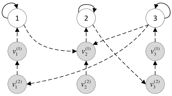
Now, we briefly explain how to use the augmented graph to address delays and asynchrony. Suppose that node sends message to node at and due to delay node receives it at time interval . However, this message is used by node at time due to asynchrony. In this case, all the edges are included in . In the augmented graph, this can be viewed as that node sends message to node via the relay nodes and , respectively. Clearly, all non-virtual nodes in receive the same information as that in and hence their updates appear to be synchronous and without delays.
In , we enumerate non-virtual nodes first and then virtual nodes. Specifically, let for all and . That is, node of is the -th node in , and the -th node in is the virtual node for all and . Let be the number of nodes of . Then, the AsySPA can be expressed as a synchronous and delay-free augmented system
| (11) | ||||
where , and , ,
| (12) |
and denotes the transmission delay from node to node at time . Under Assumption 3, for all , and for any . Finally,
| (13) |
where
| (14) |
for all .
Note that is a column-stochastic matrix. Moreover, the last equality in (11) is only for nodes in , and is well-defined because and hence for all and . In fact, the infimum of is strictly greater than as proved in the next subsection. Since for all from Assumption 1 and Lemma 1(c), we have , which is key to consensus achieving.
IV-C Asymptotic consensus among nodes
We now show that each node of the AsySPA asymptotically converges to consensus. To this end, we define
| (15) |
and
| (16) |
which is the average of elements in .
The following lemma states that converges to a rank-one matrix and implies that is strictly greater than 0 for all and .
Lemma 2
Proof:
To prove (b), two cases are separately studied. If , then , and hence the result is obtained.
If , it follows from [42, Lemma 2(b)] that for all and . Then,
| (19) | |||
| (20) | |||
| (21) |
where the last inequality follows from the column-stochasticity of . The desired result is obtained by induction.
The main result of this section ensures that all nodes of the AsySPA eventually achieve consensus.
Lemma 3
Proof:
The proof is similar to that in [6, Lemma 1] and omitted for saving space.
Lemma 3 shows that generated by the AsySPA converges to for all . Then, it is sufficient to prove that converges to an optimal solution of the DOP in (3), which is the main focus of the remaining sections.
Remark 1
The convergence rate of is a worst case bound, which has very bad scaling with respect to the number of nodes and is unfortunately achievable, see [49] for the existence of such a graph.
V Generalized Subgradient Methods
This section proposes a generalized subgradient algorithm which unifies both subgradient methods and incremental subgradient methods [43]. Then, we study its convergence, the results of which not only have its independent significance but also are essential for proving the exact convergence of the AsySPA in the next section.
We still focus on the optimization problem in (3) where the decision vector is now multi-dimensional. Given two sequences and which satisfy that
| (24) |
where for all .
Now, we propose the following generalized subgradient method to solve the optimization problem in (3)
| (25) |
where denotes noise or computing errors. The novelty of (25) lies in the use of adaptive stepsizes. By choosing different sequences and , then (25) covers a broad class of subgradient methods, e.g., the subgradient method and the incremental subgradient method as elaborated below.
Example 1 (Incremental subgradient method)
Example 2 (Subgradient method)
Now, we study the convergence of (25) under the following assumption on the sequences , and .
Assumption 4
-
(a)
There exists a such that for all .
-
(b)
There exists a such that and for all and .
-
(c)
.
Assumption 4(a) guarantees that each function in (3) needs to be updated at least once in every steps. Otherwise, will be significantly affected by some local function(s), and cannot converge to an optimal solution. Assumption 4(b) ensures that the stepsizes for updating each function should not be overwhelmingly unbalanced. Assumption 4(c) requires the cumulative noise to be bounded. Overall, Assumption 4 is reasonable and even necessary in some cases. In particular, one can easily find counterexamples where in (25) diverges if any condition in Assumption 4 is violated. Note that , and in Examples 1-2 satisfy Assumption 4 if Assumption 1 holds.
Theorem 1
Proof:
See Appendix A.
Remark 2
Due to the space limitation, we only consider diminishing stepsizes in (25). As in the standard subgradient methods, constant stepsizes can only ensure that is eventually attracted to a neighborhood of an optimal solution.
The Hölder error bound characterizes the order of growth of around an optimal solution, and holds in many applications, see [50] for details.
Theorem 2
Proof:
See Appendix B.
Theorem 2(a) reveals that in (25) can achieve a convergence rate of , which is consistent with standard subgradient methods [51, Section 3.2.3]. Theorem 2(b) cannot be directly obtained by using Theorem 2(a), which only implies that converges at the best rate of . However, Theorem 2(b) dictates that can actually converge at a rate of by using stepsizes .
VI Exact Convergence of the AsySPA
In this section, we prove the exact convergence and evaluate the convergence rate of the AsySPA.
Theorem 3
Proof:
By left-multiplying on both sides of (11), it implies
| (38) |
where is the set of activated nodes at time , i.e., . Then, two cases are considered.
Next, we evaluate the convergence rate of the AsySPA under stepsizes .
Theorem 4
Remark 3
As in Theorem 3, the global index is adopted to evaluate convergence rate. This is a common and natural way to study asynchronous algorithms, see e.g. [7, 27, 5]. Note that the convergence rate is evaluated under the worst case (c.f. Lemma 1), and in practice it may be much faster if the unevenness of update rates and delays are relatively small. One may consider to evaluate the convergence rate in terms of the running time, the maximum number of local iterations among nodes, and etc. For synchronous distributed algorithms, a lower bound on the number of communication rounds and gradient computations has been studied in [52].
In view of Theorem 4(a) and [6], it is interesting that the AsySPA essentially does not lead to any rate reduction of convergence with respect to the index . In the AsySPA, is increased by one no matter on which node has completed an update. While in the SynSPA, is increased by one only if all nodes have completed their updates, as shown in Fig. 2. That is, the SynSPA will be delayed by the slowest node. From this perspective, the computation time for increasing in the SynSPA should be longer than that of the AsySPA. In fact, the larger the asynchrony among computing nodes, the more significant improvement of the AsySPA over the SynSPA. This is also confirmed via simulation in Section VII.
Proof of Theorem 4: The proof of part (a) lies in the use of Theorem 2 on (38) or (39). We first show that there exists some such that for all . In view of Lemma 3 and , we have
| (43) | ||||
where
| (44) |
and the second inequality follows from
| (45) | ||||
Moreover, . Jointly with (LABEL:eq4_thm2) and (LABEL:eq3_thm2), the desired result follows as decreases faster than if . Part (b) can be established by using Theorem 2(b) in a similar way.
Theorem 4(b) provides a better convergence rate of the AsySPA if each local objective function further satisfies the Hölder error bound condition. However, the AsySPA usually cannot achieve linear rate even if is strongly convex with Lipschize continuous gradient. One may expect that the convergence rate of the AsySPA is lower and upper bounded by two SynSPAs. The worst case corresponds to the SynSPA in which each node updates in the same rate as that of the slowest node, and the best case is the SynSPA in which each node updates in the same rate as that of the fastest node. Since the SynSPA is unable to achieve linear rate, the AsySPA cannot neither. In our recent work [53], we show how to achieve linear rate by substantially revising the AsySPA.
VII Numerical Examples
In this section we numerically illustrate the performance of the AsySPA in distributedly training a multi-class logistic regression classifier on the Covertype dataset, which is available from the UCI machine learning repository [44] and has also been used in [7]. Moreover, we further test the algorithms on a support vector machine (SVM) training problem in Section VII-E.
The objective is to solve the optimization problem
| (47) |
where is the number of training instances, is the number of classes, is the number of features, is the feature vector of the -th instance, is the label vector of the -th instance using the one-hot encoding, is the weighting matrix to be optimized, is a regularization factor, and denotes the Frobenius norm. As in [7], we normalize non-categorical features by subtracting the mean and dividing by the standard deviation.
The problem in (47) is strictly convex. To validate the AsySPA, we adopt the Message Passing Interface (MPI) on a server to simulate a network with multiple connected nodes. Specifically, the MPI uses cores (nodes) to form a graph , and the communication among cores is configured to be directed, synchronous, or asynchronous. Each core is exclusively assigned a subset of the dataset with training instances, and hence only has a local objective function. We perform several experiments, and the source codes in Python are available on the Internet555https://github.com/jiaqi61/asyspa.
We use the averaged training error, i.e., to compare distributed algorithms under different scenarios, where is the mean of all nodes’ states at time and is an approximated optimal value of the problem (47) that is obtained from a centralized gradient descent method with sufficiently many iterations.

VII-A Comparison with centralized gradient methods
We first compare the performance of the AsySPA with the centralized gradient method.
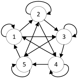
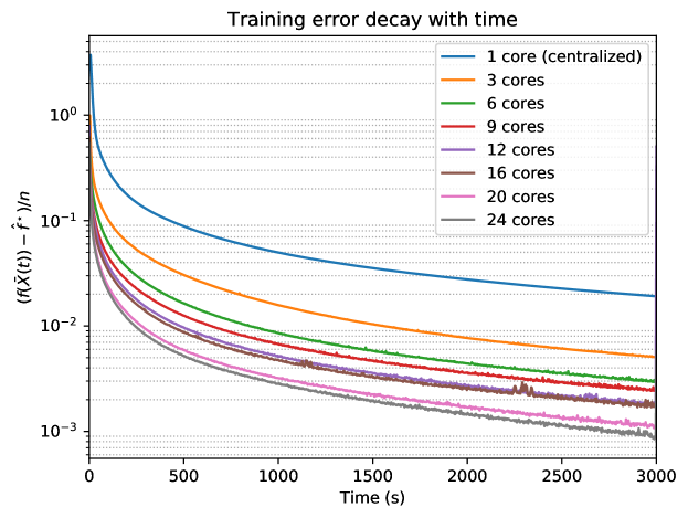
The centralized algorithm is implemented on a single core while the AsySPA is tested over core(s) with a digraph in Fig. 4. Each core computes a new update by using (7) in Algorithm 2 immediately after it finishes its current update. To accelerate computation, we set in both centralized and distributed cases, rather than the diminishing stepsizes in Assumption 1(b).
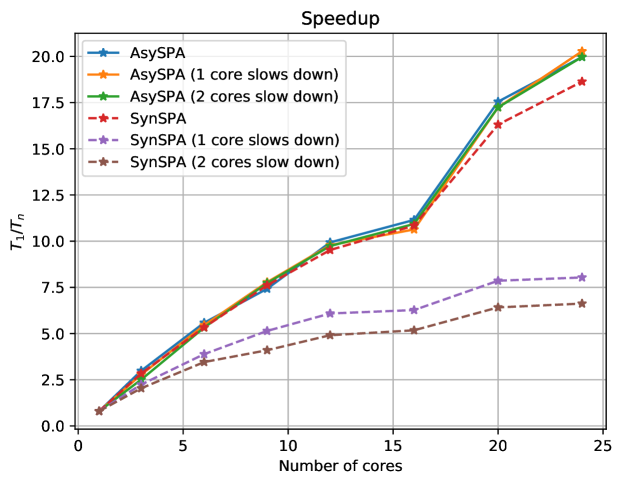
Fig. 5 depicts how the averaged training error decreases in the computing time. Clearly, the AsySPA outperforms the centralized algorithm in all experiments and the improvement is more significant if is larger. This is further illustrated in Fig. 6, where we compute the speedup defined by , and is the time when the averaged error over cores reduces to .
We also test the AsySPA over a digraph where a core can send messages to cores that are steps away as in [24], where . The results remain almost unchanged from Fig. 5. Note that nodes in this case have a smaller number of in-neighbors and hence it is more scalable. We further compare the effect of the number of neighbors in Section VII-D.
VII-B Comparison with the SynSPA
We also compare the AsySPA with the SynSPA in Algorithm 1, where the number of cores, communication digraph, and stepsize remain the same. To simulate the UUR, The -th core in the AsySPA case updates every ms (), while the -th core in the synchronous case sends messages to its out-neighbors every ms, and perform an update after all cores have received messages from their in-neighbors. Fig. LABEL:sub@fig7 shows the convergence behaviors of the AsySPA and the SynSPA. As expected, the AsySPA converges faster than the SynSPA in all cases.
To illustrate the better robustness of the AsySPA over the SynSPA, we consider the situation that some nodes slow down by adding an artificial waiting time after each update, where is an exponential distributed random variable with expectation 20ms. Fig. 6 shows the speedup of the AsySPA and the SynSPA in these experiments. Clearly, the AsySPA is almost not affected by the slowed down core(s), while the convergence rate of the SynSPA is severely reduced by the slowed down node(s).
Note that in the synchronous case the MPI acts like there is a global clock, which may be not available in practice. Moreover, the physical communication networks may have limited bandwidth and delays, which are worse than the one here inside a single computer. This makes the performance difference between the SynSPA and the AsySPA more significant.
VII-C Comparison with the-state-of-the-art algorithm in [7]
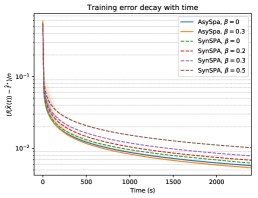
We compare the AsySPA with the asynchronous algorithm in [7] over cores, the communication digraph of which remains the same as before. Each core uses the diminishing stepsize . To simulate uneven updates of agents, we let the -th core update once every ms (), and test the algorithms for . Note that a larger leads to a higher unevenness, and means all cores update at the same rate.
Fig. 8 shows the averaged training error, where the shade area is the range that lie within. Clearly, the algorithm in [7] fails to converge to an exact optimal solution of problem (47) except for the case , and the larger , the larger gap from an optimal solution, which is consistent with [7]. In contrast, the AsySPA converges to an optimal solution in all cases, and the unevenness only affects the maximum difference among agents’ states, which however decreases to .
VII-D Effect of stepsizes and number of out-neighbors
We compare the performance of the AsySPA under different choices of stepsize. Fig. LABEL:sub@fig8 depicts the training error under constant stepsize and diminishing stepsize. Clearly, a diminishing stepsize with larger converges faster at the expense of more oscillations (the shade area), and a constant stepsize cannot guarantee the consensus among agents. This phenomenon also appears in the standard subgradient method.
We then examine the effect of the number of out-neighbors on the performance of the AsySPA. We test the AsySPA under cases that each core sends messages to itself and its next cores (c.f. Fig. 4). The results are shown in Fig. LABEL:sub@fig9. It is interesting to notice that the algorithm converges faster by increasing the number of out-neighbors until it achieves some critical number (4 in this experiment). Then the convergence rate remains almost the same or even decreases a bit as the number of out-neighbors increases. A possible reason is that while more out-neighbors lead to less iterations to achieve consensus among agents, they increase the communication overhead.
VII-E Train a support vector machine
Since the subgradient methods are very suitable for minimizing non-smooth objective functions but the logistic regression cost function is smooth, we finally test the algorithm on a SVM training problem with hinge loss, which has the following non-smooth cost function,
| (48) |
where is the integer label of the -th instance. We repeat some of the experiments in previous subsections on this problem and the result is shown in Fig. 9. We can see the performance is very similar with that on the logistic regression problem.
VIII Conclusions
This paper has proposed the AsySPA to solve the DOP over digraphs with uneven update rates and bounded transmission delays. We also demonstrated its advantages over the existing distributed algorithms. Currently, we only consider the general case that the objective function in the DOP is convex. In the future, we shall design the accelerated AsySPA for the strongly convex objective function with Lipschitz continuous gradient.
Appendix A Proof of Theorem 1
The proof can be roughly divided into 4 steps. We first show that (25) is an -subgradient step in Step 1, and derive a basic equality for the distance between and in Step 2. Then, this distance is shown to be essentially decreasing in Step 3. Finally, we prove the convergence by following a similar argument in standard subgradient methods.
Step 1: The iterate in (25) is an -subgradient step.
Let and . Clearly, it follows from Assumption 1 that for all and
| (49) |
For all , it holds that
| (50) | ||||
| (51) | ||||
| (52) | ||||
| (53) | ||||
| (54) |
Step 2: A basic equality for the distance between and .
To simplify notations, we let , and use and to denote and , respectively. It follows from Assumption 4 that for all . Then, it follows from (25) that
| (55) | ||||
where we define the sum operator as
to save space and .
Moreover, we have that
| (56) | ||||
where the first inequality uses the relation for all , for all and for all from Assumption 4. The second inequality follows from the Cauchy-Schwarz inequality. Hence, we obtain that
| (57) | ||||
Step 3: The distance between and is essentially decreasing.
Firstly, we consider the second term of the right-hand-side of (55), and obtain that
| (58) | ||||
where the first equality is from (50) and
Note that , which implies that Then, it follows from (56) and (57) that .
Secondly, we evaluate the first term of the right-hand-side of (LABEL:eq10_prop2), leading to that
| (59) | ||||
where and . In addition, , and
Thirdly, we examine the first term of the right-hand-side of (LABEL:eq11_prop2), i.e.,
| (60) | ||||
| (61) |
where the equality holds by expanding the left-hand-side with reorganization, and then uses the fact that for any from Assumption 4.
Let . It follows from Assumption 4 that and . Jointly with (60), we obtain
| (62) | ||||
where we use the fact that for all and from Assumption 4, and
| (63) | ||||
which shows that is bounded. Moreover,
| (64) | ||||
| (65) | ||||
| (66) |
which implies that , i.e., converges absolutely, and hence exists and is finite.
Finally, combining (LABEL:eq10_prop2), (LABEL:eq11_prop2) and (LABEL:eq12_prop2) yields the key inequality
| (67) | ||||
| (68) | ||||
| (69) |
where is positive. In view of (55), the distance between and is essentially decreasing in the sense of neglecting all trivial terms.
Step 4: Convergence of the iterate in (25).
Eq. (67) together with (55) implies that
| (70) | ||||
| (71) |
where . Apparently, exists and is finite.
Note that may be negative for some , and thus the convergence of and cannot be obtained directly from the supermartingale convergence theorem (SCT, [43, Proposition A.4.4]). Nonetheless, we can readily prove that is convergent and the convergence of to by using similar arguments of SCT. Together with the fact that , it implies the convergence of to .
Appendix B Proof of Theorem 2
B-A Proof of Part (a):
For convenience, we only prove the case for , while the proof extends to in a straightforward manner.
The relation (LABEL:eq2_prop2) implies that
| (74) | ||||
Since , and hence , we have
| (75) | ||||
Adding (LABEL:eq2_prop3) over implies that
| (76) |
It follows from (LABEL:eq3_prop1), the definitions of , and (63) that
| (77) | ||||
where the second to last inequality uses and the relation , and the last inequality follows from that and .
Eq. (LABEL:eq4_prop2) combined with (76) and the fact that yields
| (78) | ||||
The desired result follows by noticing that .
B-B Proof of Part (b):
Define and we can rewrite (LABEL:eq2_prop2) as
| (79) | ||||
where and hence the first inequality follows; the second inequality is from (LABEL:eq2_prop2), the third inequality uses the Hölder error bound, and the last equality follows from and thus .
The goal is to derive convergence rates for a sequence satisfying (LABEL:eq4_prop3). Note that it follows from (63) that
| (80) | ||||
Let
| (81) |
and its complement
| (82) |
It holds that for any ,
| (83) |
If is empty, then the proof completes. Otherwise, let and be two consecutive elements in () such that . We have from (LABEL:eq6_prop3) that
| (84) |
Then, it follows from (LABEL:eq4_prop3) that
| (85) | ||||
Invoking Theorem 6 in [50], we obtain that there exists a constant such that
On the other hand, (63) implies that
| (86) | ||||
| (87) | ||||
| (88) |
where is a positive constant. Thus, we have
| (89) |
which implies for some .
References
- [1] A. Nedić, A. Olshevsky, and M. G. Rabbat, “Network topology and communication-computation tradeoffs in decentralized optimization,” Proceedings of the IEEE, vol. 106, no. 5, pp. 953–976, May 2018.
- [2] R. Hannah, F. Feng, and W. Yin, “A2BCD: Asynchronous acceleration with optimal complexity,” in International Conference on Learning Representations, 2019. [Online]. Available: https://openreview.net/forum?id=rylIAsCqYm
- [3] K. Xie, Q. Cai, and M. Fu, “A fast clock synchronization algorithm for wireless sensor networks,” Automatica, vol. 92, pp. 133–142, 2018.
- [4] M. Assran and M. Rabbat, “An empirical comparison of multi-agent optimization algorithms,” in IEEE Global Conference on Signal and Information Processing, 2017, pp. 573–577.
- [5] D. P. Bertsekas and J. N. Tsitsiklis, Parallel and distributed computation: numerical methods. Athena Scientific, 2015.
- [6] A. Nedić and A. Olshevsky, “Distributed optimization over time-varying directed graphs,” IEEE Transactions on Automatic Control, vol. 60, no. 3, pp. 601–615, 2015.
- [7] M. Assran and M. Rabbat, “Asynchronous subgradient-push,” arXiv preprint arXiv:1803.08950, 2018.
- [8] A. Nedić and A. Ozdaglar, “Distributed subgradient methods for multi-agent optimization,” IEEE Transactions on Automatic Control, vol. 54, no. 1, pp. 48–61, 2009.
- [9] W. Shi, Q. Ling, G. Wu, and W. Yin, “Extra: An exact first-order algorithm for decentralized consensus optimization,” SIAM Journal on Optimization, vol. 25, no. 2, pp. 944–966, 2015.
- [10] G. Qu and N. Li, “Harnessing smoothness to accelerate distributed optimization,” IEEE Transactions on Control of Network Systems, vol. 5, no. 3, pp. 1245–1260, 2018.
- [11] J. Zhang, K. You, and T. Başar, “Distributed discrete-time optimization in multi-agent networks using only sign of relative state,” IEEE Transactions on Automatic Control, vol. 64, no. 6, pp. 2352–2367, 2019.
- [12] S. Magnússon, C. Enyioha, N. Li, C. Fischione, and V. Tarokh, “Convergence of limited communications gradient methods,” IEEE Transactions on Automatic Control, vol. 63, no. 5, pp. 1356–1371, 2018.
- [13] P. Xie, K. You, R. Tempo, S. Song, and C. Wu, “Distributed convex optimization with inequality constraints over time-varying unbalanced digraphs,” IEEE Transactions on Automatic Control, vol. 63, no. 12, pp. 4331–4337, 2018.
- [14] C. Xi and U. A. Khan, “Dextra: A fast algorithm for optimization over directed graphs,” IEEE Transactions on Automatic Control, vol. 62, no. 10, pp. 4980–4993, 2017.
- [15] A. Nedić, A. Olshevsky, and W. Shi, “Achieving geometric convergence for distributed optimization over time-varying graphs,” SIAM Journal on Optimization, vol. 27, no. 4, pp. 2597–2633, 2017.
- [16] I. Notarnicola and G. Notarstefano, “Asynchronous distributed optimization via randomized dual proximal gradient,” IEEE Transactions on Automatic Control, vol. 62, no. 5, pp. 2095–2106, 2017.
- [17] A. Nedić, “Asynchronous broadcast-based convex optimization over a network,” IEEE Transactions on Automatic Control, vol. 56, no. 6, pp. 1337–1351, 2011.
- [18] P. Bianchi, W. Hachem, and F. Iutzeler, “A coordinate descent primal-dual algorithm and application to distributed asynchronous optimization,” IEEE Transactions on Automatic Control, vol. 61, no. 10, pp. 2947–2957, 2016.
- [19] F. Farina, A. Garulli, A. Giannitrapani, and G. Notarstefano, “Asynchronous distributed method of multipliers for constrained nonconvex optimization,” in 2018 European Control Conference (ECC). IEEE, 2018, pp. 2535–2540.
- [20] E. Wei and A. Ozdaglar, “On the convergence of asynchronous distributed alternating direction method of multipliers,” in IEEE Global Conference on Signal and Information Processing, 2013, pp. 551–554.
- [21] J. Xu, S. Zhu, Y. C. Soh, and L. Xie, “Convergence of asynchronous distributed gradient methods over stochastic networks,” IEEE Transactions on Automatic Control, vol. 63, no. 2, pp. 434–448, 2018.
- [22] Z. Peng, Y. Xu, M. Yan, and W. Yin, “Arock: an algorithmic framework for asynchronous parallel coordinate updates,” SIAM Journal on Scientific Computing, vol. 38, no. 5, pp. A2851–A2879, 2016.
- [23] T. Wu, K. Yuan, Q. Ling, W. Yin, and A. H. Sayed, “Decentralized consensus optimization with asynchrony and delays,” IEEE Transactions on Signal and Information Processing over Networks, vol. 4, no. 2, pp. 293–307, 2018.
- [24] X. Lian, W. Zhang, C. Zhang, and J. Liu, “Asynchronous decentralized parallel stochastic gradient descent,” in Proceedings of the 35th Conference on Machine Learning, 2018, pp. 3049–3058.
- [25] X. Zhao and A. H. Sayed, “Asynchronous adaptation and learning over networks-Part I: Modeling and stability analysis,” IEEE Transactions on Signal Processing, vol. 63, no. 4, pp. 811–826, 2015.
- [26] N. Bof, R. Carli, G. Notarstefano, L. Schenato, and D. Varagnolo, “Multiagent newton–raphson optimization over lossy networks,” IEEE Transactions on Automatic Control, vol. 64, no. 7, pp. 2983–2990, July 2019.
- [27] Y. Tian, Y. Sun, and G. Scutari, “ASY-SONATA: Achieving linear convergence in distributed asynchronous multiagent optimization,” in 2018 56th Annual Allerton Conference on Communication, Control, and Computing (Allerton). IEEE, 2018, pp. 543–551.
- [28] J. Tsitsiklis, D. Bertsekas, and M. Athans, “Distributed asynchronous deterministic and stochastic gradient optimization algorithms,” IEEE Transactions on Automatic Control, vol. 31, no. 9, pp. 803–812, 1986.
- [29] L. Cannelli, F. Facchinei, V. Kungurtsev, and G. Scutari, “Asynchronous parallel algorithms for nonconvex optimization,” Mathematical Programming, 2019.
- [30] M. Eisen, A. Mokhtari, and A. Ribeiro, “Decentralized quasi-newton methods,” IEEE Transactions on Signal Processing, vol. 65, no. 10, pp. 2613–2628, 2017.
- [31] S. Li and T. Başar, “Asymptotic agreement and convergence of asynchronous stochastic algorithms,” IEEE Transactions on Automatic Control, vol. 32, no. 7, pp. 612–618, 1987.
- [32] T. T. Doan, C. L. Beck, and R. Srikant, “On the convergence rate of distributed gradient methods for finite-sum optimization under communication delays,” Proceedings of the ACM on Measurement and Analysis of Computing Systems, vol. 1, no. 2, pp. 37:1–37:27, 2017.
- [33] H. Wang, X. Liao, T. Huang, and C. Li, “Cooperative distributed optimization in multiagent networks with delays,” IEEE Transactions on Systems, Man, and Cybernetics: Systems, vol. 45, no. 2, pp. 363–369, 2015.
- [34] T. Yang, J. Lu, D. Wu, J. Wu, G. Shi, Z. Meng, and K. H. Johansson, “A distributed algorithm for economic dispatch over time-varying directed networks with delays,” IEEE Transactions on Industrial Electronics, vol. 64, no. 6, pp. 5095–5106, 2017.
- [35] P. Lin, W. Ren, and Y. Song, “Distributed multi-agent optimization subject to nonidentical constraints and communication delays,” Automatica, vol. 65, pp. 120–131, 2016.
- [36] P. Xie, K. You, Y. Hong, and L. Xie, “A survey of distributed convex optimization algorithms over networks,” Control Theory & Applications, vol. 35, no. 7, pp. 918–927, 2018.
- [37] Y. Sun, G. Scutari, and D. Palomar, “Distributed nonconvex multiagent optimization over time-varying networks,” in 50th Asilomar Conference on Signals, Systems and Computers, 2016, pp. 788–794.
- [38] K. I. Tsianos, S. Lawlor, and M. G. Rabbat, “Push-sum distributed dual averaging for convex optimization,” in 51st IEEE Conference on Decision and Control, Dec 2012, pp. 5453–5458.
- [39] R. Xin and U. A. Khan, “A linear algorithm for optimization over directed graphs with geometric convergence,” IEEE Control Systems Letters, vol. 2, no. 3, pp. 325–330, 2018.
- [40] A. Priolo, A. Gasparri, E. Montijano, and C. Sagues, “A distributed algorithm for average consensus on strongly connected weighted digraphs,” Automatica, vol. 50, no. 3, pp. 946–951, 2014.
- [41] K. Cai and H. Ishii, “Average consensus on general strongly connected digraphs,” Automatica, vol. 48, no. 11, pp. 2750–2761, 2012.
- [42] A. Nedić and A. Ozdaglar, “Convergence rate for consensus with delays,” Journal of Global Optimization, vol. 47, no. 3, pp. 437–456, 2010.
- [43] D. P. Bertsekas, Convex Optimization Algorithms. Athena Scientific Belmont, 2015.
- [44] D. Dheeru and E. Karra Taniskidou, “UCI machine learning repository,” 2017. [Online]. Available: http://archive.ics.uci.edu/ml
- [45] C. Xi, R. Xin, and U. A. Khan, “Add-opt: Accelerated distributed directed optimization,” IEEE Transactions on Automatic Control, vol. 63, no. 5, pp. 1329–1339, 2018.
- [46] J. Zeng and W. Yin, “Extrapush for convex smooth decentralized optimization over directed networks,” Journal of Computational Mathematics, vol. 35, no. 4, pp. 381–394, 2017.
- [47] Y. Xu, T. Han, K. Cai, Z. Lin, G. Yan, and M. Fu, “A distributed algorithm for resource allocation over dynamic digraphs,” IEEE Transactions on Signal Processing, vol. 65, no. 10, pp. 2600–2612, 2017.
- [48] J. M. Hendrickx and J. N. Tsitsiklis, “Fundamental limitations for anonymous distributed systems with broadcast communications,” in 53rd Annual Allerton Conference on Communication, Control, and Computing. IEEE, 2015, pp. 9–16.
- [49] A. Nedic, A. Olshevsky, and C. A. Uribe, “Distributed Gaussian learning over time-varying directed graphs,” in 50th Asilomar Conference on Signals, Systems and Computers, Nov 2016, pp. 1710–1714.
- [50] P. R. Johnstone and P. Moulin, “Faster subgradient methods for functions with hölderian growth,” Mathematical Programming, 2019.
- [51] Y. Nesterov, Introductory lectures on convex optimization: A basic course. Springer Science & Business Media, 2013, vol. 87.
- [52] C. A. Uribe, S. Lee, A. Gasnikov, and A. Nedić, “A dual approach for optimal algorithms in distributed optimization over networks,” arXiv preprint arXiv:1809.00710, 2018.
- [53] J. Zhang and K. You, “Asynchronous decentralized optimization in directed networks,” arXiv preprint arXiv:1901.08215, 2019.