Eigenvectors of Deformed Wigner Random Matrices

Abstract

We investigate eigenvectors of rank-one deformations of random matrices $\boldsymbol{B}=\boldsymbol{A}+\theta\boldsymbol{uu}^{*}$ in which $\boldsymbol{A}\in\mathbb{R}^{N\times N}$ is a Wigner real symmetric random matrix, $\theta\in\mathbb{R}^{+}$, and $\boldsymbol{u}$ is uniformly distributed on the unit sphere. It is well known that for $\theta>1$ the eigenvector associated with the largest eigenvalue of $\boldsymbol{B}$ closely estimates $\boldsymbol{u}$ asymptotically, while for $\theta<1$ the eigenvectors of $\boldsymbol{B}$ are uninformative about $\boldsymbol{u}$. We examine $\mathcal{O}(\frac{1}{N})$ correlation of eigenvectors with $\boldsymbol{u}$ before phase transition and show that eigenvectors with larger eigenvalue exhibit stronger alignment with deforming vector through an explicit inverse law. This distribution function will be shown to be the ordinary generating function of Chebyshev polynomials of second kind. These polynomials form an orthogonal set with respect to the semicircle weighting function. This law is an increasing function in the support of semicircle law for eigenvalues $(-2\>,+2)$. Therefore, most of energy of the unknown deforming vector is concentrated in a $cN$-dimensional ($c<1$) known subspace of $\boldsymbol{B}$. We use a combinatorial approach to prove the result.

I Introduction

Let $\boldsymbol{A}_{N\!\times\!N}$ be a random matrix deformed by a low-rank matrix $\boldsymbol{P}$ to give $\boldsymbol{B}=\boldsymbol{A}+\boldsymbol{P}$. In this scenario, $\boldsymbol{B}$ can be interpreted as the observations of a structured pure signal $\boldsymbol{P}$ contaminated by maximally unstructured noise term $\boldsymbol{A}$. The main question is whether reliable information about the signal can be extracted from noisy observations? We are usually interested in either an inference on presence of the signal or an estimate of the signal component [1]. Inference problem on the presence of an unknown signal entails examining the eigenvalues of the observation matrix $\boldsymbol{B}$, specially the largest of them in magnitude. Therefore, much effort is devoted to investigating distribution and behavior of eigenvalues of random matrices. This has been done both in the null hypothesis of a single random matrix [2, 3, 4, 5], and in the alternative hypothesis of a deformed random matrix [6, 7]. In contrast, the estimation problem involves the eigenvectors associated with the largest eigenvalues of the observation matrix.

$\boldsymbol{A}_{N\!\times\!N}$ is called a Wigner random matrix if it is symmetric real with elements $A_{ij}$ independent random variables for $i\leqslant j$ with zero mean, $\mathbb{E}A_{ij}^{2}=\frac{1}{N}$, and uniformly bounded higher moments [8]. Wigner [2], showed that the eigenvalues of such a random matrix converge to a bulk with semi-circle law on the support of $(-2\>,+2)$. Marcenko and Pastur followed a similar approach in [3], to calculate the distribution of singular values of a rectangular random matrix. When the symmetry assumption is relaxed, the complex eigenvalues exhibit a circular distribution which was observed and sketch-proved by Girko in [4]. Statistical distribution of the largest eigenvalue of $\boldsymbol{A}$ is of high importance in inference and other applications. This distribution was characterized by Tracy and Widom in [5].

In an inference scenario, a signal part may be present in the observations. Signal is a highly structured matrix in the form of a rank-one unit Ferobenius norm matrix. The observation model will be $\boldsymbol{B}=\boldsymbol{A}+\theta\boldsymbol{uu}^{*}$ in which $\theta\geqslant 0$ is the signal amplitude and $\lVert\boldsymbol{u}\rVert_{2}=1$. It is well-known that if $\theta<1$, addition of the signal makes no asymptotic change in the limiting distribution of the eigenvalues. In case $\theta>1$, a phase transition occurs meaning that the largest eigenvalue separates significantly from the bulk of the spectrum and moves from $+2$ to essentially $\theta+\frac{1}{\theta}$. This has been shown for the first time in the context of nonzero mean Wigner matrices in [9], then in Gaussian ensembles in [10], and finally as a universal result with relaxed assumptions on the random matrix in [6].

The estimation problem is associated with the eigenvectors of the observation matrix. In the null case when signal is not present, the eigenvectors of Gaussian random matrix are Haar distributed on the orthogonal group $\mathbb{O}(N)$ [8]. When unitary invariance of a Gaussian distribution is not present, a similar result [11], shows that the eigenvectors of a Wigner random matrix are delocalized in the sense that their $\ell_{p}$ norms for $p\geqslant 2$ are $\mathcal{O}(N^{\frac{1}{p}-\frac{1}{2}})$. In the deformed case of $\theta>0$, it is shown in [12] that above a certain threshold for signal eigenvalues, the observation matrix eigenvectors are partially localized in the coordinate system defined by signal eigenvectors. Assumptions on the signal in [12] is rather restrictive. A more general approach in this area is [7] in which authors demonstrate phase transition both for eigenvalues and eigenvectors of deformed general random matrix.

For a fixed rank signal, there is a threshold on the eigenvalues of the signal, above which the corresponding observation matrix eigenvalue moves out of the bulk in a position predictable by $\theta$ and Stieltjes transform of the bulk distribution. Eigenvectors are shown to possess a good alignment with the signal after phase transition. Assume a rank-one model $\boldsymbol{B}=\boldsymbol{A}+\theta\boldsymbol{uu}^{*}$ and denote eigenvalue decomposition of $\boldsymbol{A}$ and $\boldsymbol{B}$ as:

$$\boldsymbol{A}=\sum_{i=1}^{N}d_{i}\boldsymbol{\omega}_{i}\boldsymbol{\omega}_{i}^{*}$$ (1)

$$\boldsymbol{B}=\sum_{i=1}^{N}\lambda_{i}\boldsymbol{v}_{i}\boldsymbol{v}_{i}^{*}$$ (2)

in which eigenvalues are sorted $d_{1}\geqslant d_{2}\geqslant\cdots\geqslant d_{N}$ and $\lambda_{1}\geqslant\lambda_{2}\geqslant\cdots\geqslant\lambda_{N}$. Assume that $\boldsymbol{A}$ is a normalized Wigner real random matrix. Then for $\theta>1$ the largest eigenvalue of observation converges to $\lambda_{1}\overset{\text{a.s.}}{\longrightarrow}\theta+\frac{1}{\theta}$ [7, 6] and the associated eigenvector lies asymptotically on a cone around $\boldsymbol{u}$ defined by $\langle\boldsymbol{v}_{1},\boldsymbol{u}\rangle^{2}\xrightarrow{\text{a.s.}}1-\frac{1}{\theta^{2}}$ [7]. Other eigenvectors are uninformative about $\boldsymbol{u}$ and therefore $\langle\boldsymbol{v}_{i},\boldsymbol{u}\rangle^{2}\xrightarrow{\text{a.s.}}0$.

Before phase transition when $\theta<1$ every eigenvalue is in the bulk and the eigenvectors are Haar-distributed on $\mathbb{O}(N)$ and therefore $\langle\boldsymbol{v}_{i},\boldsymbol{u}\rangle^{2}\xrightarrow{\text{a.s.}}0\;:\;\forall i\leqslant N$ [7]. In fact, this inner product should sum to one and therefore it is $\mathcal{O}\big{(}\frac{1}{N}\big{)}$. From a perturbation perspective, adding the signal part increases the “energy” of the random matrix in direction $\boldsymbol{u}$. Therefore, eigenvectors associated with the largest eigenvalues should slightly rotate to interpolate between $\boldsymbol{A}$ powerful directions and $\boldsymbol{u}$. This seems to result in a non-uniform distribution of $\boldsymbol{u}$ energy in subspaces spanned by each $\boldsymbol{v}_{i}$, i.e. $\mathbb{E}\,|\langle\boldsymbol{v}_{i},\boldsymbol{u}\rangle|^{2}$. Gradually, the first eigenvectors incorporate a good portion of the energy of $\boldsymbol{u}$ and the remaining eigenvectors compete for less. Therefore most of the energy of $\boldsymbol{u}$ should be confined in a subspace spanned by eigenvectors with larger eigenvalues. In another view, adding energy in direction $\boldsymbol{u}$, increases the chance of nearby directions to win to be the eigenvectors of the largest eigenvalues. Therefore, larger eigenvalues exhibit better alignment with the signal on average. Fig. 1 shows a sample of inner products when $N=200$ and $\theta=0.7$.

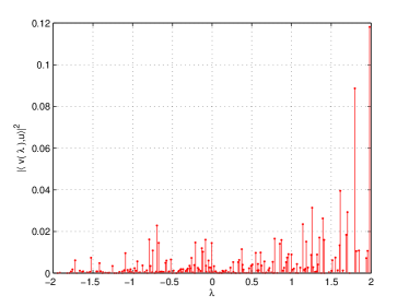
Figure 1: A sample of inner products $\langle\boldsymbol{v}(\lambda),\boldsymbol{u}\rangle^{2}$ versus $\lambda$ in which $N=200$ and $\theta=0.7$. Eigenvectors associated with larger eigenvalues are on average better aligned with $\boldsymbol{u}$.

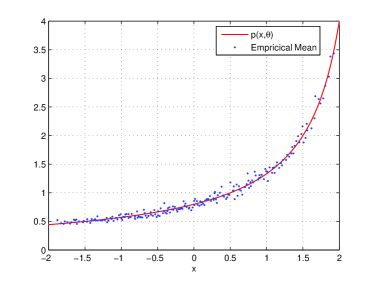
Figure 2: Empirical mean of $N\langle\boldsymbol{v}(x),\boldsymbol{u}\rangle^{2}$ and the predicted function $p(x;\theta)$ match well. Simulation parameters are $N=200$ and $\theta=0.5$ while 500 Monte Carlo iterations are used to calculate the empirical mean.

Nothing is deterministic in Fig. 1 and therefore we are interested in the expected value of inner products. Fig. 2 shows the empirical means of $\langle\boldsymbol{v}(x),\boldsymbol{u}\rangle^{2}$ in 500 Monte Carlo iterations with $N=200$ and $\theta=0.5$. In this paper, the law of distribution $\lim_{N\to+\infty}N\,\mathbb{E}\,\langle\boldsymbol{v}(x),\boldsymbol{u}\rangle^{2}$ is calculated to be:

$$p(x;\theta)\mathrel{\mathop{:}}=\frac{1}{\theta(\theta+\frac{1}{\theta}-x)}$$ (3)

which quite matches with the empirical mean in Fig. 2.

State of the art signal estimation methods are capable only when signal is stronger than noise and phase transition has occurred. Their presupposition is that before phase transition there is no data extractable about the signal which is lost below noise level. Though, (3) shows that this is not the case. Fig. 2 shows that most of the energy of the unknown signal is concentrated in the subspace spanned by first eigenvectors of the observation matrix which are known to the observer. For example, picking 100 first eigenvectors of Fig. 2 will give 70$\%$ of the energy of $\boldsymbol{u}$. It means that in a 200-dimensional space, before phase transition, we can specify a 100-dimensional subspace where the signal is mostly lie in it, which is a lot of information. In general, regarding that $p(x,\theta)$ is an increasing function with $x$ when $\theta\geqslant 0$ and for a positive constant $c\leqslant 1$ we have:

$$\sum_{i=1}^{cN}\langle\boldsymbol{v}_{i},\boldsymbol{u}\rangle^{2}\xrightarrow{\text{\; p \;}}\mathcal{P}(\theta;c)\geqslant c$$ (4)

in which $\mathcal{P}(\theta;C)\leqslant 1$ is an increasing function of $\theta\geqslant 0$.

After all, the main interesting point about $p(x;\theta)$ is its extreme simplicity in form. It only has a pole in the location which it should have. Nothing extra is present in this law. Also its similarity to the Stieltjes transform kernel seems to be inherent.

The paper is organized as follows: In section II the most relevant available results to the problem is discussed. Section III introduces our main contributions and the proofs are relegated to the appendices.

II Prior Art

In this section, we present the most relative results in the literature to our main results. These include results on eigenvalues and eigenvectors of general and random matrices. We study the spectral decomposition of a real Wigner matrix perturbed by a rank-one deformation matrix:

$$\boldsymbol{B}_{N}=\boldsymbol{A}_{N}+\theta\boldsymbol{u}_{N}\boldsymbol{u}_{N}^{*}$$ (5)

where $\boldsymbol{u}_{N}$ is a $N\times 1$ vector uniformly distributed on the unit sphere $\mathbb{S}^{N-1}$, $\theta\in\mathbb{R}^{+}$ is independent of $N$, and $\boldsymbol{A}_{N}$ is a $N\times N$ real symmetric Wigner matrix defined as:

$$\boldsymbol{A}_{N}\mathrel{\mathop{:}}=\frac{1}{\sqrt{N}}\boldsymbol{W}_{N}$$ (6)

in which $\boldsymbol{W}_{N}$ is a random matrix with the following properties:
(i) elements of $\boldsymbol{W}_{N}$ are independent up to symmetry: $\{W_{ij}\;:\;i\leqslant j\}$ are independent random variables.
(ii) symmetric distribution and zero odd moments: $\mathbb{E}W_{ij}^{2k+1}=0\;:\;\forall i,j,k$.
(iii) second moments: $\mathbb{E}W_{ij}^{2}=1$ for $i<j$ and $\mathbb{E}W_{ii}^{2}$ are uniformly bounded.
(iv) subGaussian assumption: $\forall k\quad\exists\,\beta>0\;:\;\mathbb{E}W_{ij}^{2\!k}\leqslant(\beta k)^{k}$.

In this paper, we are mainly concerned with the real setting. Although, [6] assumes an alternative complex setting:
(i’) diagonal elements are real while $\{W_{ii}\}$ and $\{\Re W_{ij}\,,\,\Im W_{ij}\,:\,i<j\}$ are independent real random variables.
(ii’) real and imaginary parts are symmetrically distributed with every odd moments zero.
(iii’) second moments $\mathbb{E}|W_{ij}|^{2}=1$ for $i<j$ and $\mathbb{E}W_{ii}^{2}$ are uniformly bounded.
(iv’) subGaussian assumption: $\forall k\quad\exists\,\beta>0\;:\;\mathbb{E}|W_{ij}|^{2\!k}\leqslant(\beta k)^{k}$.

Since the deforming matrix $\theta\boldsymbol{u}_{N}\boldsymbol{u}_{N}^{*}$ is of fixed rank (here rank-one), it will not asymptotically affect the global distribution of the eigenvalues of $\boldsymbol{B}$. The distribution is still the original Wigner semicircle law of the eigenvalues of $\boldsymbol{A}$. The empirical distribution of eigenvalues under assumptions (i)-(iv) or (i’)-(iv’) converges weakly to the probability measure:

$$\mu_{N}\mathrel{\mathop{:}}=\frac{1}{N}\sum_{i=1}^{N}\delta_{d_{i}}\xrightarrow{\text{N}\to\infty}\mu_{\textrm{sc}}$$ (7)

with corresponding density of a semicircle:

$$\frac{\mathrm{d}\mu_{\textrm{sc}}(x)}{\mathrm{d}x}=\frac{1}{2\pi}\sqrt{4-x^{2}}\,\mathbb{I}_{[-2,+2]}(x)$$ (8)

From hereafter we may omit inherent dependence of variables on $N$ for better readability. Although addition of a fixed rank perturbation does not alter the global behavior of the eigenvalues, it may strongly influence the extreme eigenvalues. The following result was first presented for Gaussian Wigner random matrices in [10], and then generalized for any subGaussian ensemble (i’)-(iv’) in [6]:

Theorem 1.

[6] For any real $t\geqslant 0$ define:

$$\rho_{\theta}\mathrel{\mathop{:}}=\theta+\frac{1}{\theta}$$ (9)

$$\sigma_{\theta}^{2}\mathrel{\mathop{:}}=1-\frac{1}{\theta^{2}}$$ (10)

$\bullet$ for $\theta>1$ :

$$\lim_{N\to\infty}\mathbb{P}\{N^{\frac{1}{2}}(\lambda_{1}-\rho_{\theta})\geqslant t\}=\frac{1}{\sqrt{2\pi}\sigma_{\theta}}\int_{-\infty}^{t}\!\!\!e^{-\frac{y^{2}}{2\sigma_{\theta}^{2}}}\textnormal{d}y$$ (11)

$\bullet$ for $\theta<1$ :

$$\lim_{N\to\infty}\mathbb{P}\{N^{\frac{2}{3}}(\lambda_{1}-2)\geqslant t\}=F_{2}^{\textnormal{TW}}(t)$$ (12)

$\bullet$ for $\theta=1$ :

$$\lim_{N\to\infty}\mathbb{P}\{N^{\frac{2}{3}}(\lambda_{1}-2)\geqslant t\}=F_{3}^{\textnormal{TW}}(t)$$ (13)

where $F_{2}^{\textnormal{TW}}$ and $F_{3}^{\textnormal{TW}}$ are Tracy-Widom distributions with 2 and 3 degrees of freedom [5].

Basically, Theorem 1 states that before and on the phase transition, the largest eigenvalue is approximately unchanged by the presence of the deforming factor, while after phase transition it is moved out of the bulk of the spectrum to its new position at $\rho_{\theta}$.

Despite the eigenvalues, little is known about the eigenvectors of deformed random matrices. Using the Stieltjes transform [13], it was shown in [7] that the eigenvectors also experience a phase transition.

Theorem 2.

[7] For $\theta\geqslant 0$ and under assumptions (i)-(iv):

$$\langle\boldsymbol{v}_{1},\boldsymbol{u}\rangle^{2}\xrightarrow{\text{a.s.}}\left\{\begin{array}[]{ll}1-\frac{1}{\theta^{2}}&\textnormal{if}\quad\theta>1\\ 0&\textnormal{if}\quad\theta\leqslant 1\end{array}\right.$$

as $N\to+\infty$.

Theorem 2 states the phase transition for eigenvectors and predicts two distinct phases for their distribution with respect to the signal component $\boldsymbol{u}$. Before phase transition no information is available about $\boldsymbol{u}$ in eigenvectors $\boldsymbol{v}_{i}$, while after phase transition a single eigenvector $\boldsymbol{v}_{1}$ bears a large amount of information about $\boldsymbol{u}$. Another relevant result about perturbation of eigenvectors of a general matrix is the Davis-Kahan inequality [14]:

Theorem 3.

(Davis-Kahan [15]) if $\boldsymbol{S}$ and $\boldsymbol{T}$ are symmetric $N\times N$ matrices and if:

$$\delta\mathrel{\mathop{:}}=\min_{j\neq i}|\lambda_{i}(\boldsymbol{S})-\lambda_{j}(\boldsymbol{S})|$$ (14)

then the angle between corresponding eigenvectors is bounded above by:

$$\sin\angle(\boldsymbol{v}_{i}(\boldsymbol{S}),\boldsymbol{v}_{i}(\boldsymbol{T}))\leqslant\frac{2\,\|\boldsymbol{S}-\boldsymbol{T}\|}{\delta}$$ (15)

Suppose that in Theorem 3 we set $\boldsymbol{S}\mathrel{\mathop{:}}=\boldsymbol{B}$ and $\boldsymbol{T}\mathrel{\mathop{:}}=\theta\boldsymbol{uu}^{*}$. Since $\|\boldsymbol{A}\|\simeq 2$ and the level spacing between eigenvalues of $\boldsymbol{B}$ is of $\mathcal{O}(\frac{1}{N})$ before phase transition, Davis-Kahan gives an upper bound of $\mathcal{O}(N)$ in (15) which is useless.

III Main Results

In this section the main results of this paper is presented while proofs are relegated to the appendices. In the low-rank deformation problem for random matrices, the distribution of the first eigenvectors are well known after phase transition [7]. Though, little is known about the situation before phase transition. This is because of the premise that eigenvectors “individually” might carry useful information about the signal subspace. In this regard, Theorem 2 shows that this information is zero asymptotically. But simulation results e.g. Fig. 1 exhibit a random structure in correlations of eigenvectors with the signal $\boldsymbol{u}$. Although this information is $\mathcal{O}(\frac{1}{N})$, it follows a very smooth increasing expected value which can aggregate information of $\mathcal{O}(N)$ first eigenvectors to achieve a meaningful information about the signal $\boldsymbol{u}$. Therefore, it is useful to study this small correlation.

Theorem 4.

For a rank-one deformation model of (5) and under assumptions (i)-(iv) for the Wigner matrix $\boldsymbol{A}$:

$$p(x;\theta)\mathrel{\mathop{:}}=\lim_{N\to\infty}N\,\mathbb{E}\,\langle\boldsymbol{v}(x),\boldsymbol{u}\rangle^{2}=\frac{1}{\theta(\theta+\frac{1}{\theta}-x)}$$ (16)

in which $\boldsymbol{v}(x)$ is the eigenvector of $\boldsymbol{B}$ corresponding to eigenvalue $x$.

Proof.

See Appendix A. ∎

Remark 5.

The distribution function in Theorem 4 is surprisingly equal to the ordinary generating function of the Chebyshev polynomials of second kind $U_{k}(\frac{x}{2})$. These polynomials form an orthogonal set of polynomials with an inner product weighted by the semicircle function.

Function $p(x;\theta)$ has a simple pole at $\theta+\frac{1}{\theta}$. Therefore, any eigenvalue located around this value will get a large inner product $\langle\boldsymbol{v}(\theta+\frac{1}{\theta}),\boldsymbol{u}\rangle^{2}=\mathcal{O}(1)$ while other eigenvalues exhibit $\mathcal{O}(\frac{1}{N})$ inner products. Before phase transition, every eigenvalue is in the bulk of semicircle law supported on $(-2,+2)$ while $\theta+\frac{1}{\theta}$ is outside of this interval. For $\theta=1$, as $N\rightarrow+\infty$ we have $\lambda_{1}\xrightarrow{\text{a.s.}}2$ [8], and therefore $\mathbb{E}\langle\boldsymbol{v}_{1},\boldsymbol{u}\rangle^{2}$ will become large. This means that (3) predicts the phase transition of $\boldsymbol{v}_{1}$ at $\theta=1$. Now suppose that $\theta>1$ and we will have an eigenvalue located around $\theta+\frac{1}{\theta}$ [7]. Then (16) predicts that $\boldsymbol{v}_{1}$ is well-aligned with $\boldsymbol{u}$. Therefore, (16) describes the eigenvectors behavior before, after, and on the phase transition.

Theorem 4 can be used to describe the distribution of the eigenvectors of the deformed random matrix both before and after phase transition in a single law. Although the mean value of correlations are smooth, their samples exhibit a random behavior. Therefore, to estimate a subspace close to $\boldsymbol{u}$, sufficient number of first eigenvectors should be incorporated in a span. This subspace will contribute a concentrated portion of energy of $\boldsymbol{u}$ larger than its proportional dimension:

Theorem 6.

For a single matrix $\boldsymbol{B}$ abiding model (5) and under assumptions (i)-(iv) on $\boldsymbol{A}$:

$$\sum_{i=1}^{cN}\langle\boldsymbol{v}_{i},\boldsymbol{u}\rangle^{2}\xrightarrow{\;\;\textnormal{p}\;\;}\mathcal{P}(\theta;c)\geqslant c$$ (17)

where $c\leqslant 1$ is a positive constant and the function $\mathcal{P}(\theta;c)$ is an increasing function of both $c$ and $\theta$:

$$\mathcal{P}(\theta;c)\mathrel{\mathop{:}}=\int_{m}^{2}\mu_{\textnormal{sc}}(x)p(x;\theta)\textnormal{d}x$$ (18)

in which $m$ is a threshold defined implicitly via:

$$c=\int_{m}^{2}\mu_{\textnormal{sc}}(x)\textnormal{d}x$$ (19)

Proof.

See Appendix B. ∎

Remark 7.

Theorem 6 paves the way for using Theorem 4 in practice using a sum in the spectrum which concentrates around the expected value. In practice, only one sample of the deformed matrix is available and therefore, we cannot use a mean value to approach the expected value. Theorem 6 gives an alternative way for averaging by incorporating large number of stronger eigenvectors to achieve a good estimate of the signal subspace.

Appendix A Proof of Theorem 4

We are interested in inner products of the eigenvectors of $\boldsymbol{B}$ and $\boldsymbol{u}$. The classical Wigner proof [2], for the semicircle distribution of the eigenvalues of a symmetric random matrix used traces of the random matrix and its powers. Trace of $k^{\textnormal{th}}$ power of the matrix corresponds to the $k^{\textnormal{th}}$ moment of its eigenvalues distribution. We use the same idea to calculate the distribution of the inner products. To produce such inner products multiply $\boldsymbol{B}$ by $\boldsymbol{u}$ from left and right:

$$\boldsymbol{u}^{*}\boldsymbol{Bu}=\sum_{i=1}^{N}\lambda_{i}\langle\boldsymbol{v}_{i},\boldsymbol{u}\rangle^{2}$$ (20)

The same can be done for the $k^{\textnormal{th}}$ power of $\boldsymbol{B}$:

$$\boldsymbol{u}^{*}\boldsymbol{B}^{k}u=\sum_{i=1}^{N}\lambda_{i}^{k}\langle\boldsymbol{v}_{i},\boldsymbol{u}\rangle^{2}$$ (21)

These are linear combinations of the inner products. These quadratic forms have been used in the literature to show localization properties of eigenvectors of random matrices [19]. Assume that phase transition is not occurred and then the distribution of $\lambda_{i}$ is known. Therefore, we are able to deduce distribution of the inner products from sufficient different linear combinations in the form of (21). Using the model in (5), we can calculate the value of linear combinations e.g. (20) in terms of $\theta$:

$$\boldsymbol{u}^{*}\!\boldsymbol{Bu}=\boldsymbol{u}^{*}(\boldsymbol{A}+\theta\boldsymbol{u}\boldsymbol{u}^{*})\boldsymbol{u}=\boldsymbol{u}^{*}\!\boldsymbol{Au}+\theta$$ (22)

The second equality comes from the fact that $\boldsymbol{u}^{*}\boldsymbol{u}=1$. Since $\boldsymbol{u}$ is uniformly distributed on the unit sphere $\mathbb{S}^{N-1}$ and $\boldsymbol{A}$ is a subGaussian random matrix, the product form $\boldsymbol{u}^{*}\boldsymbol{Au}$ is concentrated around its mean. The following Lemma states the result:

Lemma 8.

For a Wigner matrix $\boldsymbol{A}$ with assumptions (i)-(iv) and $\boldsymbol{u}$ uniformly distributed on the unit sphere $\mathbb{S}^{N-1}$ and $k\in\mathbb{N}\cup\{0\}$:

$$\boldsymbol{u}^{*}\!\boldsymbol{A}^{k}u\xrightarrow{\;\;\textnormal{p}\;\;}\left\{\begin{array}[]{ll}c_{{k}/{2}}&k:\;\textnormal{even}\\ 0&k:\;\textnormal{odd}\end{array}\right.$$ (23)

as $N\to\infty$ and $c_{k}$ is the $k^{\textnormal{th}}$ Catalan number:

$$c_{k}\mathrel{\mathop{:}}=\frac{1}{k+1}\left(\!\!\!\begin{array}[]{c}2k\\ \!k\end{array}\!\!\!\right)$$

Proof.

See Appendix C. ∎

Before phase transition $\lambda_{i}$’s are in the bulk spectrum with spacing of $\mathcal{O}(\frac{1}{N})$. Assuming that the expected values of the inner products in (21) is a smooth function of the eigenvalues, we will have the following Lemma:

Lemma 9.

the quadratic form in (21) converges in probability to its mean value:

$$\boldsymbol{u}^{*}\boldsymbol{B}^{k}u\xrightarrow{\;\;\textnormal{p}\;\;}\int\mu_{\textnormal{sc}}(x)x^{k}p(x;\theta)\textnormal{d}x$$ (24)

in which

$$p(x;\theta)\mathrel{\mathop{:}}=N\mathbb{E}\{\langle\boldsymbol{v}(x),\boldsymbol{u}\rangle^{2}|x\}$$ (25)

Proof.

See Appendix D. ∎

The distribution function $p(x;\theta)$ is assumed to be a smooth function of $x$ and $\theta$. Therefore, it has a Taylor series with respect to $\theta$:

$$p(x;\theta)=\sum_{k=0}^{\infty}\theta^{k}f_{k}(x)$$ (26)

Combinatorial calculations show that $f_{k}(x)$ are Chebyshev polynomials of second kind. These polynomials form an orthogonal polynomial set with respect to the weight function of the semicircle law $\mu_{\textnormal{sc}}(x)$, in the interval $[-2\,,+2]$. The first few functions are:

$$f_{0}(x) = 1$$

$$f_{1}(x) = x$$

$$f_{2}(x) = x^{2}-1$$

$$f_{3}(x) = x^{3}-2x$$

$$f_{4}(x) = x^{4}-3x^{2}+1$$ (27)

Lemma 10.

Polynomials $f_{k}(x)$ of the Taylor series expansion of the distribution function $p(x;\theta)$ are described as:

$$f_{k}(x)=U_{k}\left(\frac{x}{2}\right)$$ (28)

in which $U_{k}(x)$ is the Chebyshev polynomial of second kind.

Proof.

See Appendix E. ∎

Therefore, the distribution function $p(x;\theta)$ is the ordinary generating function of Chebyshev polynomials of second kind which is known to be [16]:

$$p(x;\theta)=\sum_{k=0}^{\infty}\theta^{k}U_{k}\left(\frac{x}{2}\right)=\frac{1}{1-\theta x+\theta^{2}}$$ (29)

for $|\theta|<1$ which is equivalent to (16).

Appendix B Proof of Theorem 6

To show convergence of the summation to its limit in probability, we first show that the limit is the expected value of the sum and then investigate the second moment.

Lemma 11.

Under the assumptions of Theorem 6:

$$\mathbb{E}\sum_{i=1}^{cN}\langle\boldsymbol{v}_{i},\boldsymbol{u}\rangle^{2}=\mathcal{P}(\theta;c)$$ (30)

Proof.

The sum in (30) can be converted to:

$$\sum_{i=1}^{cN}\langle\boldsymbol{v}_{i},\boldsymbol{u}\rangle^{2}=\sum_{i=1}^{N}\langle\boldsymbol{v}_{i},\boldsymbol{u}\rangle^{2}\,\mathbb{I}(\lambda_{i}\geqslant\lambda_{cN})$$ (31)

in which $\mathbb{I}(\cdot)$ is the indicator function. Whatever $\theta$ is, $\lambda_{cN}$ converges in probability to $m$ which is defined implicitly by (19). Using the techniques of the proof of Lemma 13 in Appendix D, the expected value of (31) will be

$$\mathbb{E}\,\sum_{i=1}^{cN}\langle\boldsymbol{v}_{i},\boldsymbol{u}\rangle^{2} \xrightarrow{\;\;\textnormal{p}\;\;}\frac{1}{N}\sum_{i=1}^{N}\,\mathbb{E}\,\{\mathbb{I}(\lambda_{i}\geqslant m)\,\mathbb{E}\,\{N\langle\boldsymbol{v}_{i},\boldsymbol{u}\rangle^{2}|\lambda_{i}\}\}$$ (32)

$$=\quad\frac{1}{N}\sum_{i=1}^{N}\,\mathbb{E}\,\{\mathbb{I}(\lambda_{i}\geqslant m)\,p(\lambda_{i};\theta)\}$$ (33)

$$\xrightarrow{\;\;\textnormal{p}\;\;}\int\mu_{\textnormal{sc}}(x)\,\mathbb{I}(x\geqslant m)\,p(x;\theta)\textnormal{d}x$$ (34)

$$=\quad\int_{m}^{2}\mu_{\textnormal{sc}}(x)\,p(x;\theta)\textnormal{d}x=\mathcal{P}(\theta;c)$$ (35)

where in (34) we have used the fact that asymptotically, the empirical measure of eigenvalues converges weakly in probability to the semi-circle law. Note that the above results are valid only for $c<1$. ∎

Lemma 9 states that $\boldsymbol{u}^{*}\boldsymbol{B}^{k}\boldsymbol{u}$ converges in probability to its mean. Define the empirical probability measure and its mean as:

$$L_{N}\mathrel{\mathop{:}} =\sum_{i=1}^{N}\delta_{\lambda_{i}}\langle\boldsymbol{v}_{i},\boldsymbol{u}\rangle^{2}$$ (36)

$$\langle\bar{L}_{N},f\rangle\mathrel{\mathop{:}} =\mathbb{E}\,\langle L_{N},f\rangle\quad\forall f\in C_{b}$$ (37)

Then, $\boldsymbol{u}^{*}\boldsymbol{B}^{k}\boldsymbol{u}=\langle L_{N},x^{k}\rangle$ and Lemma 9 asserts that

$$\lim_{N\to\infty}\langle L_{N},x^{k}\rangle=\langle\,\mu_{\textnormal{sc}}(x)\,p(x;\theta),x^{k}\rangle$$ (38)

Although function $\mathbb{I}(x\geqslant m)$ is not continuous, a deliberately exact approximation of it can be formed by a truncated Taylor series expansion in the interval $[-2,+2]$. Therefore we can conclude that

$$\lim_{N\to\infty} \sum_{i=1}^{cN}\langle\boldsymbol{v}_{i},\boldsymbol{u}\rangle^{2}=\lim_{N\to\infty}\langle L_{N},\mathbb{I}(x\geqslant m)\rangle=$$ (39)

$$\langle\,\mu_{\textnormal{sc}}(x)\,p(x;\theta),\mathbb{I}(x\geqslant m)\rangle=\mathcal{P}(\theta;c)$$ (40)

which is the result of Theorem 6.

Appendix C Proof of Lemma 8

We show that $\boldsymbol{u}^{*}\boldsymbol{A}^{k}\boldsymbol{u}$ concentrates around its mean:

$$\mathbb{E}\,\boldsymbol{u}^{*}\boldsymbol{A}^{k}\boldsymbol{u}=\mathbb{E}\,\textnormal{Tr}\,(\boldsymbol{u}^{*}\boldsymbol{A}^{k}\boldsymbol{u})=\mathbb{E}\,\textnormal{Tr}\,(\boldsymbol{A}^{k}\boldsymbol{u}\boldsymbol{u}^{*})=$$

$$\mathbb{E}_{\boldsymbol{A}}\,\mathbb{E}_{\boldsymbol{u}}\{\textnormal{Tr}\,(\boldsymbol{A}^{k}\boldsymbol{uu}^{*})\,|\boldsymbol{A}\}=\mathbb{E}_{\boldsymbol{A}}\,\textnormal{Tr}\,(\boldsymbol{A}^{k}\,\mathbb{E}_{\boldsymbol{u}}\boldsymbol{uu}^{*})$$

$$=\mathbb{E}\,\textnormal{Tr}\,(\boldsymbol{A}^{k}\frac{1}{N}\boldsymbol{I}_{N})=\mathbb{E}\,\frac{1}{N}\textnormal{Tr}\boldsymbol{A}^{k}$$ (41)

which is $c_{k/2}$ when $k$ is even and $0$ otherwise. In (C) we have used the fact that a random vector uniformly distributed on the unit sphere $\mathbb{S}^{N-1}$ is isotropic [15] and therefore $\mathbb{E}\,\boldsymbol{uu}^{*}=\frac{1}{N}\boldsymbol{I}_{N}$.

Now we give a Gaussian comparison and upper bound for product moments of $\boldsymbol{u}$:

Lemma 12.

if $\boldsymbol{u}\sim\textnormal{unif}(\mathbb{S}^{N-1})$ and $\boldsymbol{x}\sim\mathcal{N}(0,\frac{1}{N}\boldsymbol{I}_{N})$ are two random vectors then:

$$\mathbb{E}\,u_{i}^{2}u_{j}^{2}\leq\mathbb{E}\,x_{i}^{2}x_{j}^{2}=\left\{\begin{array}[]{lrl}3/N^{2}&\textnormal{if}&i=j\\ 1/N^{2}&\textnormal{if}&i\neq j\end{array}\right.$$ (42)

Proof.

Although $\boldsymbol{u}$ is a sub-Gaussian random vector [15], this is not enough to infer (42). Moments of sub-Gaussian random vectors are bounded above by Gaussian moments times a constant while in (42) the constant is unity.

General product moments of uniform distribution on unit sphere is derived in [20]:

$$\mathbb{E}\prod_{i=1}^{N}u_{i}^{k_{i}}=\frac{\Gamma(\frac{N}{2})}{2^{k}\,\Gamma(\frac{N+k}{2})}\,\prod_{i=1}^{N}\frac{k_{i}!}{(\frac{k_{i}}{2})!}$$ (43)

in which $k=\sum_{i=1}^{N}k_{i}$ and every $k_{i}$ should be an even number. Therefore, for the four’th moment we will have:

$$\mathbb{E}\,u_{i}^{4}=\frac{\Gamma(\frac{N}{2})}{2^{4}\,\Gamma(\frac{N}{2}+2)}\,\frac{4!}{2!}=\frac{3}{N^{2}+2N}\leqslant\frac{3}{N^{2}}=\mathbb{E}\,x_{i}^{4}$$ (44)

and the product moment $i\neq j$ will be bounded as:

$$\mathbb{E}\,u_{i}^{2}u_{j}^{2}=\frac{1}{N^{2}+2N}\leqslant\frac{1}{N^{2}}=\mathbb{E}\,x_{i}^{2}x_{j}^{2}$$ (45)

and the lemma is proved. ∎

Next, we examine the second moment of $\boldsymbol{u}^{*}\boldsymbol{A}^{k}\boldsymbol{u}$ to show concentration around its mean. Define $\boldsymbol{F}\mathrel{\mathop{:}}=\boldsymbol{A}^{k}$:

$$\mathbb{E}\,(\boldsymbol{u}^{*}\!\boldsymbol{A}^{k}\boldsymbol{u})^{2}=\mathbb{E}\left(\sum_{i,j}u_{i}F_{ij}u_{j}\right)^{2}=$$

$$\mathbb{E}\sum_{i,j,m,n}u_{i}u_{j}u_{m}u_{n}F_{ij}F_{mn}$$ (46)

Although elements of $\boldsymbol{u}$ are not independent random variables, it can be shown that the expected value of any combination of its elements with odd powers is zero due to the symmetry in the sphere [15]. The surviving terms are:

$$\mathbb{E}\bigg{(}\sum_{i}u_{i}^{4}F_{ii}^{2}+\sum_{i,j\neq i}u_{i}^{2}u_{j}^{2}F_{ii}F_{jj}+$$

$$\quad\quad\sum_{i,j\neq i}u_{i}^{2}u_{j}^{2}F_{ij}^{2}+\sum_{i,j\neq i}u_{i}^{2}u_{j}^{2}F_{ij}^{2}\bigg{)}$$ (47)

corresponding to situations where $(i=j=m=n)$, $(i=j,m=n)$ , $(i=m,j=n)$, and $(i=n,j=m)$ in (C). We have also used the fact that $\boldsymbol{F}$ is a symmetric matrix. Using upper bounds in Lemma 12 for the expectation on $\boldsymbol{u}$ we get:

$$\mathbb{E}\,(\boldsymbol{u}^{*}\!\boldsymbol{A}^{k}\boldsymbol{u})^{2}\quad\quad\quad\quad\quad\quad\quad\quad\quad\quad\quad\quad\quad\quad\quad\quad$$

$$\leqslant\mathbb{E}\frac{1}{N^{2}}\bigg{(}3\sum_{i}F_{ii}^{2}+\sum_{i\neq j}F_{ii}F_{jj}+2\sum_{i\neq j}F_{ij}^{2}\bigg{)}$$

$$=\mathbb{E}\frac{1}{N^{2}}\bigg{(}\sum_{i,j}F_{ii}F_{jj}+2\sum_{i,j}F_{ij}^{2}\bigg{)}\quad\quad\quad\quad$$

$$=\mathbb{E}\bigg{(}\frac{1}{N}\textnormal{Tr}\boldsymbol{A}^{k}\bigg{)}^{2}+\mathbb{E}\frac{2}{N^{2}}\,\textnormal{Tr}\boldsymbol{A}^{2k}\quad\quad\quad\quad$$

$$\xrightarrow{\;\;\textnormal{p}\;\;}\bigg{(}\mathbb{E}\frac{1}{N}\textnormal{Tr}\boldsymbol{A}^{k}\bigg{)}^{2}+\frac{2}{N}c_{k}\quad\quad\quad\quad$$ (48)

in which, the convergence in probability is due to Wigner in its proof of semi circle law [8]. Therefore:

$$\textnormal{Var}(\boldsymbol{u}^{*}\!\boldsymbol{A}^{k}\boldsymbol{u})\leqslant\frac{2}{N}c_{k}$$ (49)

Now, a standard Chebychev inequality shows concentration around the mean value in (C):

$$\mathbb{P}(|\boldsymbol{u}^{*}\!\boldsymbol{A}^{k}\boldsymbol{u}-\mathbb{E}\,\boldsymbol{u}^{*}\!\boldsymbol{A}^{k}\boldsymbol{u}|\geqslant t)\leqslant\frac{\frac{2}{N}c_{k}}{t^{2}}\xrightarrow{N\to\infty}0$$ (50)

for each fixed $t$ and therefore, convergence in probability to the mean value is proved.

Appendix D Proof of Lemma 9

We will show that $\boldsymbol{u}^{*}\boldsymbol{B}^{k}\boldsymbol{u}$ converges in probability to its expected value.

Lemma 13.

The expected value of the quadratic form is:

$$\mathbb{E}\,\boldsymbol{u}^{*}\boldsymbol{B}^{k}\boldsymbol{u}=\int\mu_{\textnormal{sc}}(x)\,x^{k}p(x;\theta)\,\textnormal{d}x$$ (51)

in which

$$p(x;\theta)\mathop{:}=\lim_{N\to\infty}\mathbb{E}\,\{N\langle\boldsymbol{v}_{i},\boldsymbol{u}\rangle^{2}|\lambda_{i}=x\}$$ (52)

Proof.

Left Hand Side of (51) can be written as:

$$\mathbb{E}\,\sum_{i=1}^{N}\langle\boldsymbol{v}_{i},\boldsymbol{u}\rangle^{2}\lambda_{i}^{k}=\frac{1}{N}\sum_{i=1}^{N}\mathbb{E}\,\{\lambda_{i}^{k}\,\mathbb{E}\,\{N\langle\boldsymbol{v}_{i},\boldsymbol{u}\rangle^{2}|\lambda_{i}\}\}$$ (53)

We assume that the inner expectation is a smooth function $p(\lambda_{i};\theta)$ with a Taylor series expansion $\sum_{\ell}\lambda_{i}^{\ell}p_{\ell}(\theta)$. Therefore, we reach to

$$\frac{1}{N}\sum_{i,\ell}\mathbb{E}\,\lambda_{i}^{k+\ell}p_{\ell}(\theta)=\sum_{\ell}p_{\ell}(\theta)\frac{1}{N}\sum_{i=1}^{N}\mathbb{E}\,\lambda_{i}^{k+\ell}$$ (54)

It is known that whatever $\theta$ is, the limiting behavior of the eigenvalues of $\boldsymbol{B}$ obeys the semi-circle law [6], since the deformation is of finite rank and energy. Therefore, the right-hand-side in (54) converges in probability to

$$\sum_{\ell}p_{\ell}(\theta)\int\mu_{\text{sc}}(x)\,x^{k+\ell}\textnormal{d}x$$ (55)

and we will have

$$\mathbb{E}\,\boldsymbol{u}^{*}\boldsymbol{B}^{k}\boldsymbol{u}=\int\mu_{\text{sc}}(x)\,x^{k}p(x;\theta)\,\textnormal{d}x$$ (56)

∎

To show convergence to the mean value, it will be sufficient to show the same for the second moment of the quadratic form:

Lemma 14.

The second moment of the quadratic form converges in probability to square of its mean value:

$$\mathbb{E}\,(\boldsymbol{u}^{*}\boldsymbol{B}^{k}\boldsymbol{u})^{2}\xrightarrow{\quad\textnormal{p}\quad}(\,\mathbb{E}\,\boldsymbol{u}^{*}\boldsymbol{B}^{k}\boldsymbol{u})^{2}$$ (57)

Proof.

expanding the terms of quadratic form we have:

$$(\boldsymbol{u}^{*}\boldsymbol{B}^{k}\boldsymbol{u})^{2}=\boldsymbol{u}^{*}(\boldsymbol{A}+\theta\boldsymbol{uu}^{*})^{k}\boldsymbol{u}\boldsymbol{u}^{*}(\boldsymbol{A}+\theta\boldsymbol{uu}^{*})^{k}\boldsymbol{u}$$ (58)

Using $\boldsymbol{u}^{*}\boldsymbol{u}=1$, (58) reduces to a summation of product forms $\theta^{k_{0}}(\boldsymbol{u}^{*}\boldsymbol{A}^{k_{1}}\boldsymbol{u})\cdots(\boldsymbol{u}^{*}\boldsymbol{A}^{k_{\ell}}\boldsymbol{u})$. In Lemma 8 we have shown that each individual term converges in probability to its mean value. Therefore, their product will also converge in probability to the product of the mean values. The same is true for the R.H.S. of (57) and therefore the L.H.S. converges to the R.H.S. in probability. ∎

Appendix E Proof of Lemma 10

We first derive $f_{0}(x)$ and $f_{1}(x)$ and then show that $f_{k}(x)$ obey a recurrence equation which is characteristic of the Chebyshev polynomials of second kind [17].

E-A Calculating $f_{0}(x)$

The inner product $\boldsymbol{u}^{*}\boldsymbol{B}^{2k}\boldsymbol{u}=\boldsymbol{u}^{*}(\boldsymbol{A}+\theta\boldsymbol{uu}^{*})^{2k}\boldsymbol{u}$ admits a polynomial expansion in which the $\theta^{0}$ term is equal to

$$\boldsymbol{u}^{*}\boldsymbol{A}^{2k}\boldsymbol{u}\xrightarrow{\quad\textnormal{p}\quad}c_{k}$$ (59)

by Lemma 8. $\boldsymbol{u}^{*}\boldsymbol{B}^{2k}\boldsymbol{u}$ also converges to an integral form which is stated in Lemma 9 and gives rise to $\theta^{0}$ term of:

$$\int\mu_{\text{sc}}(x)\,x^{2k}f_{0}(x)\textnormal{d}x.$$ (60)

$2k^{\textnormal{th}}$ moments of the semicircle law is known to be the Catalan number $c_{k}$ while the odd moments are zero. Therefore, a Taylor expansion on $f_{0}(x)$:

$$f_{k}(x)=\sum_{i=0}^{\infty}a_{ki}x^{i}$$ (61)

applied in (60) and equating to (59) gives:

$$a_{00}c_{k}+a_{02}c_{k+1}+a_{04}c_{k+2}+\cdots\equiv c_{k}\quad\forall k\in\mathbb{N}$$ (62)

and therefore, $a_{00}=1$ while $a_{0(2k)}=0$ for all $k\geqslant 1$. In the same manner $\boldsymbol{u}^{*}\boldsymbol{B}^{2k+1}\boldsymbol{u}$ gives rise to $\theta^{0}$ term of $\boldsymbol{u}^{*}\boldsymbol{A}^{2k+1}\boldsymbol{u}\xrightarrow{\;\textnormal{p}\;}0$ which should be equal to the integral form of the Taylor series:

$$a_{01}c_{k+1}+a_{03}c_{k+2}+a_{05}c_{k+3}+\cdots\equiv 0\quad\forall k\in\mathbb{N}$$ (63)

which leads to $a_{0(2k+1)}=0$ and finally we will have:

$$f_{0}(x)=1=U_{0}\left(\frac{x}{2}\right)$$ (64)

in which, $U_{0}(x)$ is the zero${}^{\textnormal{th}}$ Chebyshev polynomial of second kind.

E-B Calculating $f_{1}(x)$

Calculating $f_{1}(x)$ amounts to the $\theta^{1}$ term of $\boldsymbol{u}^{*}(\boldsymbol{A}+\theta\boldsymbol{uu}^{*})^{2k+1}\boldsymbol{u}$. The general term of this binomial expansion with only one $\theta$ term is $(\boldsymbol{u}^{*}\boldsymbol{A}^{n}\theta\boldsymbol{u})(\boldsymbol{u}^{*}\boldsymbol{A}^{2k-n}\boldsymbol{u})\xrightarrow{\quad\textnormal{p}\quad}c_{\frac{n}{2}}c_{k-\frac{n}{2}}$ when $n=2m$ is an even number $0\leqslant n\leqslant 2k$ according to Lemma 8. Therefore, sum of these general terms will give the $\theta^{1}$ coefficient as:

$$\sum_{m=0}^{k}c_{m}c_{k-m}=c_{k+1}$$ (65)

by the well-known recurrence of Catalan numbers [8]. The integral form on the Taylor series expansion of $f_{1}(x)$ gives the following equivalence:

$$a_{11}c_{k+1}+a_{13}c_{k+2}+a_{15}c_{k+3}+\cdots\equiv c_{k+1}\quad\forall k\in\mathbb{N}$$ (66)

which leads to $a_{11}=1$ and $a_{1(2k+1)}=0$ for all $k\geqslant 1$.

To determine even coefficients we consider $\boldsymbol{u}^{*}(\boldsymbol{A}+\theta\boldsymbol{uu}^{*})^{2k}\boldsymbol{u}$. From $2k$ selections between $\boldsymbol{A}$ and $\theta(\boldsymbol{uu}^{*})$, one of them is $\theta$ and the general term of interest is $(\boldsymbol{u}^{*}\boldsymbol{A}^{n}\theta\boldsymbol{u})(\boldsymbol{u}^{*}\boldsymbol{A}^{2k-1-n}\boldsymbol{u})$ in which $0\leqslant n\leqslant 2k-1$. Here it is impossible that both $n$ and $2k-1-n$ be even numbers. Therefore, the equivalence of the integral form and the combinatorial term will be:

$$a_{10}c_{k}+a_{12}c_{k+1}+a_{14}c_{k+2}+\cdots\equiv 0\quad\forall k\in\mathbb{N}$$ (67)

which gives $a_{1(2k)}=0$. Therefore, we will have:

$$f_{1}(x)=x=U_{1}\left(\frac{x}{2}\right)$$ (68)

E-C Recurrence of $f_{n}(x)$

Chebyshev polynomials of second kind satisfy the following recurrence equation:

$$U_{n}(x)=2\,xU_{n-1}(x)-U_{n-2}(x)$$ (69)

Therefore, we should prove a similar recurrence on $f_{n}(x)$:

$$f_{n}(x)=xf_{n-1}(x)-f_{n-2}(x)$$ (70)

Define $H(m,n)$ as the coefficient of $\theta^{n}$ in the inner product $\boldsymbol{u}^{*}(\boldsymbol{A}+\theta\boldsymbol{uu}^{*})^{m}\boldsymbol{u}$. We can show a recurrence on $H(m,n)$:

$$H(m,n)=H(m+1,n-1)-H(m,n-2)$$ (71)

To show (71), assume a sequence of elements $A$ and $\theta$ with length $m$. We are interested in the sum of all sequences with predetermined number of $\theta$’s while runs of $A$ should be even and each run of $A^{2n}$ is translated to $c_{n}$. For example:

$$AA\theta AAAA\theta AAAAAA\longrightarrow c_{1}c_{2}c_{3}$$ (72)

Therefore, sum of all sequences with $n$ elements of $\theta$ and total length $m$ is $H(m,n)$. To further translate the problem to a combinatorial object enumeration, we use the fact that the Catalan number $c_{k}$ counts the number of Dyck paths with length $2k$. Dyck paths are bernouli $\pm 1$ random walks which are always above the horizontal zero level and starting and ending in zero level. Therefore, transformation (72) amounts to counting the number of paths with a Dyck path of length 2, then a horizontal zero level (h) step forward, then a Dyck path of length 4 ($D_{4}$), h, and finally a $D_{6}$. Total number of such paths with $n$ h-steps and total length $m$ is $H(m,n)$. Dyck paths are bound to even length. For ease of notation, define $I_{mn}$ as the number of paths with total length of Dyck paths $2m$ and number of h-steps $n$. Note that h-steps can only occur in the zero level. Fig. 3 shows an example of such a path.

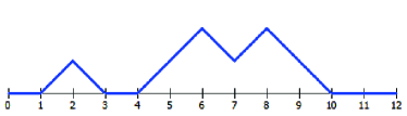
Figure 3: A sample path with total length 12 from which 4 steps are h-steps while 8 steps are Dyck $\pm 1$ steps. h-steps only occur in the zero level. Number of all such paths with 4 h-steps and $2\times 4$ Dyck steps are denoted as $I_{4,4}=H(12,4)$.

Dyck paths are equivalent to planar trees. In fact each Dyck path determines a unique planar tree by the following construction: Start from zero level and add a root node. With each up step add a new edge and the corresponding node to the tree and move up the tree to the new node. With each down step move down one node. For the paths with h-steps define a second type of dashed edges and add a dashed edge and a new node each time a h-step occurred. Therefore, our paths correspond to some planar trees connected in order by dashed edges from root nodes. An example of such trees is depicted in Fig. 4 which is equivalent to the path in Fig. 3.

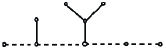
Figure 4: The tree equivalent to the path in Fig. 3. The path starts from left, goes up when reaching a solid tree, come down the tree and then again to the right.

We use analytic combinatorics [18] to show that $I_{mn}$ satisfies the following recurrence:

$$I_{mn}=I_{(m+1)(n-1)}-I_{(m+1)(n-2)}$$ (73)

for $m\geqslant 0$ and $n\geqslant 2$. Associate variable $x$ to each solid edge in the compound tree and variable $y$ to each dashed edge. A planar tree is a node with a sequence of trees attached to it. In fact trees are recursive combinatorial objects. As an example consider sequences of object $x$ regardless of their length:

$${\mathcal{S}\textnormal{EQ}}(x)\mathrel{\mathop{:}}=\{\phi,x,xx,xxx,\cdots\}$$ (74)

in which $\phi$ is the null sequence. These sequences correspond to a generating function in which power of $x$ determines number of $x$’s in the sequence:

$$\textsc{Seq}(x)\mathrel{\mathop{:}}=\frac{1}{1-x}=1+x+x^{2}+x^{3}+\cdots$$ (75)

In the same manner, sequences of $x$ and $y$’s are demonstrated using the following generating function:

$$\textsc{Seq}(x,y)\mathrel{\mathop{:}}=\frac{1}{1-x-y}=\sum_{n=0}^{\infty}(x+y)^{n}$$ (76)

since each sequence with length $n$ corresponds to a binomial expansion of $(x+y)^{n}$.

Planar trees are sequences of planar trees attached to a single root node:

$$\mathcal{T}(x)\mathrel{\mathop{:}}=\epsilon\;\mathcal{S}\textnormal{EQ}(\mathcal{T}(x))$$ (77)

in which $\epsilon$ is the root node. Therefore, the generating function of a planar tree is:

$$\textsc{T}(x)=\frac{1}{1-\textsc{T}(x)}$$ (78)

which gives:

$$T(x)=\frac{1}{2}\left(1-\sqrt{1-4x}\right)$$ (79)

Our paths are sequences of solid planar trees and dashed edges:

$$\textnormal{W}(x,y)=\frac{1}{1-y-\frac{1}{2}\left(1-\sqrt{1-4x}\right)}$$ (80)

Number of paths with $m$ solid edges and $n$ dashed edges is the coefficient of $x^{m}y^{n}$ in Taylor series expansion of $W(x,y)$ and therefore:

$$W(x,y)=\sum_{m,n=0}^{\infty}I_{mn}x^{m}y^{n}$$ (81)

The recurrence in (73) can be shown on the explicit form of $W(x,y)$ in (80). The problem is that (73) is only valid for $n\geqslant 2$. If we define number of paths with $-1$ dashed paths zero $I_{m(-1)}=0$, then (73) will be valid for $n\geqslant 1$. Therefore, (73) is equivalent to:

$$W-W_{:0}=\frac{y}{x}(W-W_{0:})-\frac{y^{2}}{x}(W-W_{0:})$$ (82)

in which $W_{:0}=W(x,y=0)$ is the coefficient of $y^{0}$ in Taylor series of $W(x,y)$ and $W_{0:}=W(x=0,y)$ is the coefficient of $x^{0}$. (82) is easily verifiable. This gives (73) and then (71). $H(m,n)$ was defined in (71) as the sum of coefficients of $\theta^{n}$ in $\boldsymbol{u}^{*}\boldsymbol{B}^{m}\boldsymbol{u}$ and therefore is equal to the integral form in Lemma 9 and we will have:

$$\int x^{m}f_{n}\textnormal{d}\mu_{\textnormal{sc}}=\int x^{m+1}f_{n-1}\textnormal{d}\mu_{\textnormal{sc}}-\int x^{m}f_{n-2}\textnormal{d}\mu_{\textnormal{sc}}$$ (83)

for all $m\geqslant 0$ and fixed $n\geqslant 2$. This completes the proof of (70) and Lemma 10.

References

- [1] R. V. Hogg, A. Craig, and J. W. McKean, Introduction to mathematical statistics, Pearson, ed., 2004.
- [2] E. Wigner, “Characteristic vectors of bordered matrices with infinite dimensions,” Ann. of Math., vol. 62, pp. 548-564, 1955.
- [3] V. A. Marcenko and L. A. Pastur, “Distribution of eigenvalues in certain sets of random matrices,” Math. USSR Sb., vol. 1, pp. 457-483, 1967.
- [4] V. L. Girko, “The circular law,” Theory Probab. Appl., vol. 29, pp. 694-706, 1984.
- [5] C. A. Tracy and H. Widom, “Level-spacing distributions and the Airy kernel,” Phys. Lett. B, vol. 305, pp. 115-118, 1993.
- [6] D. Feral and S. Peche, “The largest eigenvalue of rank one deformation of large Wigner matrices,” Comm. Math. Phys., vol. 272, pp. 185-228, 2007.
- [7] F. Benaych-Georges and R. R. Nadakuditi, “The eigenvalues and eigenvectors of finite, low rank perturbations of large random matrices,” Adv. in Math., vol. 227, pp. 494-521, 2011.
- [8] G. W. Anderson, A. Guionnet, and O. Zeitouni, An introduction to random matrices, Cambridge University Press, 2009.
- [9] Z. Furedi and J. Komlos, “The eigenvalues of random symmetric matrices,” Combinatorica, vol. 1, pp. 233-241, 1981.
- [10] S. Peche, “The largest eigenvalues of small rank perturbations of Hermitian random matrices,” Prob. Theo. Rel. Fields, vol. 134, pp. 127-174, 2006.
- [11] L. Erdos, B. Schlein, and H. T. Yau, “Semicircle law on short scales and delocalization of eigenvectors for random matrices,” Ann. of Probab. vol. 37, pp. 815-852, 2009.
- [12] J. O. Lee and K. Schnelli, “Extremal eigenvalues and eigenvectors of deformed Wigner matrices,” Prob. Theo. Rel. Fields, vol. 164, pp. 165-241, 2016.
- [13] Z. Bai and J. W. Silverstein, Spectral analysis of large dimensional random matrices, Springer, 2010.
- [14] C. Davis and W. M. Kahan, “Some new bounds on perturbation of subspaces,” Bull. Am. Math. Soc., vol. 75, pp. 863-868, 1969.
- [15] R. Vershynin, High-dimensional probability: an introduction with applications in data science, 2017.
- [16] C. Cesarano, “Identities and generating functions on Chebyshev polynomials,” Georg. Math. J., vol. 19, pp. 427-440, 2012.
- [17] T. J. Rivlin, The Chebyshev polynomials, John Wiley Sons, 1974.
- [18] P. Flajolet and R. Sedgewick, Analytic combinatorics, Cambridge University Press, 2009.
- [19] K. Wang, Optimal upper bound for the infinity norm of eigenvectors of random matrices, Ph.D. dessertation, State University of New Jersey, 2013.
- [20] K.T. Fang, S. Kotz, and K.W. Ng, Symmetric Multivariate and Related Distributions, Chapman and Hall, London, 1990.