$\epsilon_{K}$ and $\epsilon^{\prime}/\epsilon$ in a diquark model

Abstract

Based on the calculations using the lattice QCD by the RBC-UKQCD collaboration and a large $N_{c}$ dual QCD, the resulted $\epsilon^{\prime}/\epsilon$, which is less than the experimental data by more than a $2\sigma$ in the standard model (SM), suggests the necessity of a new physics effect. In order to complement the insufficient $\epsilon^{\prime}/\epsilon$, we study the extension of the SM with a colored scalar in a diquark model. In addition to the pure diquark box diagrams, it is found that the box diagrams with one $W$-boson and one diquark, ignored in the literature, play an important role in the $\Delta S=2$ process. The mass difference between $K_{L}$ and $K_{S}$ in the diquark model is well below the current data, whereas the Kaon indirect CP violation $\epsilon_{K}$ gives a strict constraint on the new parameters. Three mechanisms are classified in the study of $\epsilon^{\prime}/\epsilon$. They include a tree-level diagram, QCD and electroweak (EW) penguins, and chromomagnetic operators (CMOs). Taking the Kobayashi-Maskawa phase as the unique CP source, we analyze each contribution of the three mechanisms in detail and conclude that with the exception of QCD and EW penguins, the tree and CMO effects can singly enhance $\epsilon^{\prime}/\epsilon$ to be of ${\cal O}(10^{-3})$, depending on the values of free parameters, when the bound from $\epsilon_{K}$ is satisfied.

I Introduction

It is known that the measured CP violation in $K$ and $B$ meson decays can be attributed to the unique CP phase of the Cabibbo-Kobayashi-Maskawa (CKM) matrix Cabibbo:1963yz ; Kobayashi:1973fv in the standard model (SM). However, it is a long-standing challenge to theoretically predict the Kaon direct CP violation $\epsilon^{\prime}/\epsilon$ in the SM. Now, the progress in predicting $\epsilon^{\prime}/\epsilon$ has taken one step forward based on two results: one is from lattice QCD calculations and the other is a QCD theory-based approach.

Firstly, the RBC-UKQCD collaboration recently reported the surprising lattice QCD results on the matrix elements of $K\to\pi\pi$ and $\epsilon^{\prime}/\epsilon$ Boyle:2012ys ; Blum:2011ng ; Blum:2012uk ; Blum:2015ywa ; Bai:2015nea , where the the electroweak (EW) penguin contribution to $\epsilon^{\prime}/\epsilon$ and the Kaon direct CP violation are, respectively, shown as Blum:2015ywa ; Bai:2015nea :

$$Re(\epsilon^{\prime}/\epsilon)_{\rm EWP}=-(6.6\pm 1.0)\times 10^{-4}\,,\quad Re(\epsilon^{\prime}/\epsilon)=1.38(5.15)(4.59)\times 10^{-4}\,;$$ (1)

however, the experimental average measured by the NA48 Batley:2002gn and KTeV AlaviHarati:2002ye ; Abouzaid:2010ny is $Re(\epsilon^{\prime}/\epsilon)=(16.6\pm 2.3)\times 10^{-4}$. As a result, the lattice calculations indicate that the SM prediction is $2.1\sigma$ below the experimental value.

Using a large $N_{c}$ dual QCD (DQCD) approach Buras:2015xba ; Buras:2015yba , which was developed by Buras:1985yx ; Bardeen:1986vp ; Bardeen:1986uz ; Bardeen:1986vz ; Bardeen:1987vg , the calculations of $Re(\epsilon^{\prime}/\epsilon)$ in the QCD based approach support the RBC-UKQCD results, and the results are given as:

$$Re(\epsilon^{\prime}/\epsilon)_{\rm SM} =\left\{\begin{array}[]{c}(8.6\pm 3.2)\times 10^{-4}\,,~{}~{}\text{(}B^{(1/2)}_{6}=B^{(3/2)}_{8}=1)\,,\\ (6.0\pm 2.4)\times 10^{-4}\,,~{}~{}\text{(}B^{(1/2)}_{6}=B^{(3/2)}_{8}=0.76)\,,\end{array}\right.$$ (4)

where $B^{(1/2)}_{6}$ and $B^{(3/2)}_{8}$ denote the non-perturbative parameters of the gluon ($Q_{6}$) and EW ($Q_{8}$) penguin operators, respectively. Regardless of what the correct values of $B^{1/2}_{6}$ and $B^{3/2}_{8}$ are, the predicted $Re(\epsilon^{\prime}/\epsilon)_{\rm SM}$ also is over $2\sigma$ below the data. Although the uncertainty of $B^{(1/2)}_{6}$ is still large, it is found that both approaches obtain consistent values in $B^{(1/2)}_{6}$ and $B^{(3/2)}_{8}$ as Buras:2015xba :

$$B^{(1/2)}_{6}(m_{c})=0.57\pm 0.19\,,\ B^{(3/2)}_{8}(m_{c})=0.76\pm 0.05~{}~{}\text{(RBC-UKQCD)}\,,$$

$$B^{(1/2)}_{6}\leq B^{(3/2)}<1\,,\ B^{(3/2)}_{8}(m_{c})=0.80\pm 0.1\,.~{}~{}~{}~{}~{}~{}~{}~{}~{}~{}~{}\text{(large $N_{c}$)}\,.$$ (5)

If the RBC-UKQCD results of $B^{(1/2)}_{6}(m_{c})=0.57\pm 0.19$ and $B^{(3/2)}_{8}(m_{c})=0.76\pm 0.05$ are used, the Kaon direct CP violation becomes Buras:2015yba :

$$Re(\epsilon^{\prime}/\epsilon)_{\rm SM}=(1.9\pm 4.5)\times 10^{-4}\,,$$ (6)

where the DQCD’s value is even closer to the RBC-UKQCD result shown in Eq. (1). Moreover, using the lattice QCD results, the authors in Kitahara:2016nld also obtained a consistent result with $Re(\epsilon^{\prime}/\epsilon)=(1.06\pm 5.07)\times 10^{-4}$ at the next-leading order (NLO) corrections.

Since the DQCD result arises from the short-distance (SD) four-fermion operators, it is of interest to find other mechanisms that can complement the insufficient $\epsilon^{\prime}/\epsilon$, in the SM, such as the long-distance (LD) final state interactions (FSIs). However, the conclusion of the LD contribution is still uncertain, where the authors in Buras:2016fys obtained a negative conclusion, but the authors in Gisbert:2017vvj obtained $Re(\epsilon^{\prime}/\epsilon)=(15\pm 7)\times 10^{-4}$ when the SD and LD effects were included. On the other hand, in spite of the large uncertainty of the current lattice calculations, if we take the RBC-UKQCD’s central value as the tendency of the SM, the alternative source to enhance $\epsilon^{\prime}/\epsilon$ can be from a new physics effect Buras:2015qea ; Buras:2015yca ; Buras:2015kwd ; Buras:2015jaq ; Tanimoto:2016yfy ; Buras:2016dxz ; Kitahara:2016otd ; Endo:2016aws ; Bobeth:2016llm ; Cirigliano:2016yhc ; Endo:2016tnu ; Bobeth:2017xry ; Crivellin:2017gks ; Bobeth:2017ecx ; Haba:2018byj ; Buras:2018lgu ; Chen:2018ytc ; Chen:2018vog ; Matsuzaki:2018jui ; Haba:2018rzf ; Aebischer:2018rrz ; Aebischer:2018quc ; Aebischer:2018csl .

To explore new physics contributions to the $\epsilon^{\prime}/\epsilon$ and the Kaon indirect CP violation $\epsilon_{K}$, in this work, we investigate the diquark effects, where the diquark is a colored scalar and can originate from grand unified theories (GUTs) Barr:1986ky ; Barr:1989fi . Even without GUTs, basically, a diquark is allowed in the $SU(3)_{C}\times SU(2)_{L}\times U(1)_{Y}$ gauge symmetry, and its representation in the symmetry group depends on the coupled quark-representation Assad:2017iib . In this study, we concentrate on the color triplet and $SU(2)_{L}$ singlet diquark.

Although the diquark effects on $\epsilon_{K}$ and $\epsilon^{\prime}/\epsilon$ were investigated in Barr:1989fi , some new diquark characteristics are found in this study, which can be summarized as follows: (a) the $SU(2)_{L}$ singlet diquark can couple to the left-handed doublet and right-handed singlet quarks simultaneously. (b) When the sizable top-quark mass is taken into account, the $\Delta S=2$ box diagrams with the intermediates of $W$-boson (including charged Goldstone boson) and diquark become significant, in which the effects were ignored in  Barr:1989fi . (c) New scalar-scalar and tensor-tensor operators for $\Delta S=1$ are induced at the tree level; due to large mixings between the scalar and tensor operators, the $\epsilon^{\prime}/\epsilon$ is dominated by the isospin $I=2$ amplitude, which is produced by the tensor-tensor operators Aebischer:2018rrz . (d) QCD and EW penguin diagrams are included in $\epsilon^{\prime}/\epsilon$, and with the renormalization group (RG) effect, it is found that the $I=2$ amplitude, induced by the $Q_{8}$ operator, become dominant. (e) Chromomagnetic operators (CMOs) generated from the gluon-penguin diagrams are considered based on the matrix elements obtained in Buras:2018lgu .

Although the involved new free parameters generally can carry CP phases, in this work, we assume that the origin of the CP violation is still from the Kobayashi-Maskawa (KM) phase of the CKM matrix. This assumption can be removed if necessary. Hence, it can be concluded that $\epsilon^{\prime}/\epsilon$ can be significantly enhanced by the diquark effects when the bound from $\epsilon_{K}$ is satisfied. In addition, since rare $B$-meson processes, such as $B^{0}_{q}-\bar{B}^{0}_{q}$ ($q=d,s$) mixings, involve different parameters, e.g. $g^{R,L}_{33}$, which are irrelevant to the current study, we do not discuss the $B$-meson physics in this study.

The paper is organized as follows: In Section II, we introduce the diquark Yukawa couplings to the SM quarks and gauge couplings to the gluons, $\gamma$, and $Z$-boson. In Section III, we derive the diquark-induced effective Hamiltonian for the $\Delta S=1$ and $\Delta S=2$ processes, where the used three-point vertex functions of $d\to sg^{(*)},\gamma^{(*)},Z^{(*)}$ are derived in the appendix. The hadronic effects for the $K\to\pi\pi$ decays and the $K^{0}-\bar{K}^{0}$ transition are shown in Section IV. We also summarize the formulations of $\epsilon^{\prime}/\epsilon$ and $\epsilon_{K}$ from various operators in this section. The constraints from $\Delta S=2$ are shown in Section V. The detailed numerical analysis on $\epsilon^{\prime}/\epsilon$ based on various different mechanisms is given in Section VI. A summary is given in Section VII.

II Color-triplet diquark Yukawa and gauge couplings

In this section, we introduce the diquark Yukawa couplings and gauge couplings to the gauge bosons, including the gluons, photon, and $Z$-boson. Based on $SU(3)_{C}$ gauge invariance, it can be seen that the involving diquarks from the Yukawa sector can be color-triplet and -sextet due to $3\times 3=\bar{3}+6$. From the $SU(2)_{L}$ gauge invariance, the diquark candidates can be the $SU(2)_{L}$ singlet and triplet Barr:1989fi . In order to provide a detailed study on the diquark effects, we thus focus on the $SU(2)_{L}$ singlet and color-triplet diquark Barr:1989fi .

It can be found that the possible diquark candidates in the $SU(3)_{C}\times SU(2)_{L}\times U(1)_{Y}$ gauge group are $(\bar{3},1,1/3)$ and $(\bar{3},1,-2/3)$. For $(\bar{3},1,-2/3)$, the Yukawa couplings to the quarks are:

$$f_{ij}d^{T}_{i}CP_{R}{\bf H}^{\dagger}_{3}d_{j}+H.c.\,,$$ (7)

where $C=i\gamma^{2}\gamma^{0}$ is the charge conjugation; $P_{R(L)}=(1\pm\gamma_{5})/2$, and $f_{ij}=-f_{ji}$ due to $d^{T}_{j}\,C\,P_{R}{\bf H}^{\dagger}_{3}d^{T}_{i}=-d^{T}_{i}\,C\,P_{R}{\bf H}^{\dagger}_{3}d_{j}$. As a result, the $\Delta S=2$ process and $\epsilon^{\prime}/\epsilon$ both arise from one-loop effects. Thus, it may not be possible to explain the $\epsilon^{\prime}/\epsilon$ data when the parameters are constrained by $\epsilon^{\rm exp}_{K}$. In addition, since the involved quarks inside the loop are the down-type quarks, due to no heavy quark enhancement, e.g. $m^{2}_{t}/m^{2}_{H_{3}}$, the effects are expected to be relatively small. Hence, in this work, we devote ourselves to the ${\bf H}_{3}(\bar{3},1,1/3)$ contributions to the $\Delta S=1$ and $\Delta S=2$ processes.

II.1 Yukawa couplings

The gauge invariant Yukawa couplings of ${\bf H}_{3}(\bar{3},1,1/3)$ to the quarks in the SM gauge symmetry can be written as:

$$-{\cal L}_{Y}=f_{ij}Q^{T}_{i}C\boldsymbol{\varepsilon}{\bf H}^{\dagger}_{3}P_{L}Q_{j}+g^{R}_{ij}u^{T}_{i}C{\bf H}^{\dagger}_{3}P_{R}d_{j}+H.c,$$ (8)

where the indices $i,j$ denote the flavor indices; $\boldsymbol{\varepsilon}$ is a $2\times 2$ antisymmetric matrix with $\boldsymbol{\varepsilon}_{12}=-\boldsymbol{\varepsilon}_{21}=1$, and the representation of color-triplet diquark in $SU(3)_{C}$ can be expressed as ${\bf H}_{3}=K^{a}H^{a}_{3}$ with $(K^{a})^{ij}=1/\sqrt{2}\epsilon^{aij}$. For the complex conjugate state, we use $(\bar{K}_{a})_{ij}=(K^{a})^{ji}$, i.e. ${\bf H}^{\dagger}_{3}=\bar{K}_{a}H^{*}_{3a}$; thus, we obtain $Tr(K^{a}\bar{K}_{b})=\delta^{a}_{b}$ and $(K^{a})^{\beta\alpha}(\bar{K}_{a})_{\rho\sigma}=1/2(\delta_{\sigma}^{\beta}\delta_{\rho}^{\alpha}-\delta_{\rho}^{\beta}\delta_{\sigma}^{\alpha})$. The explicit matrix forms of $K^{a}$ ($a=1,2,3$) can be found in Han:2009ya . From Eq. (8), the color-gauge transformation of ${\bf H_{3}}$ in $SU(3)_{C}$ follows:

$${\bf H}^{\prime}_{3}=U{\bf H}_{3}U^{T}\,.$$ (9)

If we decompose the $SU(2)_{L}$ quark doublet, the left-handed quark couplings can be formed as:

$$f_{ij}u^{T}_{i}C{\bf H}^{\dagger}_{3}P_{L}d_{j}-f_{ji}d^{T}_{j}C{\bf H}^{\dagger}_{3}P_{L}u_{i}=(f_{ij}+f_{ji})u^{T}_{i}C{\bf H}^{\dagger}_{3}P_{L}d_{j}\,,$$ (10)

where the flavor indices $i,j$ do not sum. From the result, it can be seen that the color-triplet diquark Yukawa couplings to the left-handed quarks are symmetric in flavor space, i.e. $g^{L}_{ij}\equiv f_{ij}+f_{ji}=g^{L}_{ji}$. Using the new coupling definition, Eq. (8) can be written as:

$$-{\cal L}_{Y}=u^{T}_{i}C\bar{K}_{a}\left(g^{L}_{ij}P_{L}+g^{R}_{ij}P_{R}\right)d_{j}H^{*}_{3a}+H.c.$$ (11)

We will use the Yukawa couplings $g^{L,R}_{ij}$ to show the diquark effects.

II.2 Gluon couplings

In order to calculate the gluon-penguin diagrams for the $d\to sg^{(*)}$ transition, we need to know the gluon couplings to the diquark. Since the diquark state carries two color indices, the associated gauge covariant derivative will be different from that of fundamental representation of $SU(3)_{C}$. To find the covariant derivative of ${\bf H}_{3}$ in $SU(3)_{C}$, we first consider the gauge transformation of $\partial_{\mu}{\bf H}_{3}$. Using Eq. (9) and $U=\exp(ig_{s}\boldsymbol{\alpha})=\exp(ig_{s}\alpha^{a}T^{a})$, in which $T^{a}=\lambda^{a}/2$ and $\lambda^{a}$ are the Gell-Mann matrices, the color-gauge transformation of $\partial_{\mu}{\bf H}_{3}$ can be expressed as:

$$\partial_{\mu}{\bf H}^{\prime}_{3}=U\left(\partial_{\mu}{\bf H}_{3}+ig_{s}\partial_{\mu}\boldsymbol{\alpha}{\bf H}_{3}+ig_{s}{\bf H}_{3}\partial_{\mu}\boldsymbol{\alpha}^{T}\right)U^{T}\,.$$ (12)

It can be seen that there are two terms related to $\partial_{\mu}\boldsymbol{\alpha}$; that is, $(\partial_{\mu}\boldsymbol{\alpha}){\bf H}_{3}$ and ${\bf H}_{3}\partial_{\mu}\boldsymbol{\alpha}^{T}$. From the result, we can define the covariant derivative of ${\bf H}_{3}$, which transforms as ${\bf H}_{3}$ in $SU(3)_{C}$ symmetry, as:

$$D_{\mu}{\bf H}_{3}\equiv\partial_{\mu}{\bf H}_{3}+ig_{s}{\bf A}_{\mu}{\bf H}_{3}+ig_{s}{\bf H}_{3}{\bf A}^{T}_{\mu}\,,$$ (13)

where ${\bf A}_{\mu}=T^{a}A^{a}_{\mu}$ denotes the gluon fields, and its gauge transformation is given by ${\bf A}^{\prime}_{\mu}=U{\bf A}_{\mu}U^{\dagger}-\frac{i}{g_{s}}U\partial_{\mu}U^{\dagger}$. We have checked that the identity $D^{\prime}_{\mu}{\bf H}^{\prime}_{3}=UD_{\mu}{\bf H}_{3}U^{T}$ is satisfied under the $SU(3)_{C}$ transformation.

After finding $D_{\mu}{\bf H}_{3}$, the $SU(3)_{C}$ gauge invariant kinetic term of ${\bf H}_{3}$ can thus be written and expanded as:

$$Tr(D_{\mu}{\bf H}_{3})^{\dagger}(D^{\mu}{\bf H}_{3}) =\partial_{\mu}H^{*}_{3a}\partial^{\mu}H^{a}_{3}+ig_{s}Tr\partial_{\mu}{\bf H}^{\dagger}_{3}\left({\bf A}_{\mu}{\bf H}_{3}+{\bf H}_{3}{\bf A}^{T}_{\mu}\right)$$

$$-ig_{s}Tr\left({\bf H}^{\dagger}_{3}{\bf A}_{\mu}+{\bf A}^{T}_{\mu}{\bf H}^{\dagger}_{3}\right)\partial_{\mu}{\bf H}_{3}$$

$$+g^{2}_{s}Tr\left({\bf H}^{\dagger}_{3}{\bf A}_{\mu}+{\bf A}^{T}_{\mu}{\bf H}^{\dagger}_{3}\right)\left({\bf A}_{\mu}{\bf H}_{3}+{\bf H}_{3}{\bf A}^{T}_{\mu}\right)\,.$$ (14)

We can read out the gluon couplings to the diquark-pair from the second and third terms, where their color factors can be factored out as:

$${\cal L}_{{\bf A}H_{3}H_{3}} =ig_{s}\left(Tr\bar{K}_{a}T^{A}K^{b}+Tr\bar{K}_{a}K^{b}(T^{A})^{T}\right)(\partial^{\mu}H^{*}_{3a})H^{b}_{3}A^{A}_{\mu}$$

$$-ig_{s}\left(Tr\bar{K}_{a}T^{A}K^{b}+Tr\bar{K}_{a}K^{b}(T^{A})^{T}\right)H^{*}_{3a}(\partial^{\mu}H^{b}_{3})A^{A}_{\mu}\,.$$ (15)

It can be easily shown that $Tr\bar{K}_{a}K^{b}(T^{A})^{T}=Tr\bar{K}_{a}T^{A}K^{b}$, and the interaction of ${\bf A}_{\mu}H_{3}H_{3}$ can then be rewritten as:

$${\cal L}_{{\bf A}H_{3}H_{3}}=ig_{s}(t^{A})^{b}_{a}\left[(\partial^{\mu}H^{*}_{3a})H^{b}_{3}A^{A}_{\mu}-H^{*}_{3a}(\partial^{\mu}H^{b}_{3})A^{A}_{\mu}\right]\,,$$ (16)

with $(t^{A})^{b}_{a}=2Tr(\bar{K}_{a}T^{A}K^{b})$. As a result, the associated Feynman rule can be obtained as:

$$A^{A}_{\mu}H^{*}_{3a}H^{b}_{3}:-ig_{s}(t^{A})^{b}_{a}(p_{b}+p_{a})_{\mu}\,.$$ (17)

Additionally, the color trace factors $Tr\bar{K}_{a}T^{A}K^{b}$ indeed are related to the generators of $SU(3)_{C}$, and the relationship can be built as follows:

$$Tr\bar{K}_{a}T^{A}K^{b} =(\bar{K}_{a})_{\alpha\beta}(T^{A})_{\rho}^{\beta}(K^{b})^{\rho\alpha}=\frac{1}{2}\epsilon_{a\beta\alpha}\epsilon^{b\rho\alpha}(T^{A})_{\rho}^{\beta}$$

$$=\frac{1}{2}\left(\delta_{a}^{b}Tr(T^{A})-(T^{A})^{b}_{a}\right)=-\frac{(T^{A})^{b}_{a}}{2}\,,$$ (18)

where $\epsilon_{ijk}\epsilon^{\ell mk}=\delta_{i}^{\ell}\delta_{j}^{m}-\delta_{i}^{m}\delta_{j}^{\ell}$ and $Tr(T^{A})=0$ are used.

II.3 Photon and $Z$-boson gauge couplings

Since ${\bf H}_{3}$ is an $SU(2)_{L}$ singlet, the ${\bf H}_{3}$ hypercharge is equal to its electric charge. In order to know the photon and $Z$-boson gauge couplings to the diquark, we write the $U(1)_{Y}$ covariant derivative of ${\bf H}_{3}$ as:

$$D_{\mu}{\bf H}_{3}=(\partial_{\mu}+ig^{\prime}Y_{H_{3}}B_{\mu}){\bf H}_{3}\,,$$ (19)

where $g^{\prime}$ is the $U(1)_{Y}$ gauge coupling constant; $Y_{H_{3}}$ is the ${\bf H}_{3}$ hypercharge, and $B_{\mu}$ is the $U(1)_{Y}$ gauge field. The $U(1)_{Y}$ gauge invariant kinetic term of ${\bf H}_{3}$ can then be expressed as:

$$Tr(D_{\mu}{\bf H}_{3})^{\dagger}(D^{\mu}{\bf H_{3}}) =(D_{\mu}H^{*}_{3a})(D^{\mu}H^{a}_{3})=\partial_{\mu}H^{*}_{3a}\partial^{\mu}H^{a}_{3}$$

$$+ig^{\prime}Y_{H_{3}}\left(\partial_{\mu}H^{*}_{3a}H^{a}_{3}-H^{*}_{3a}\partial_{\mu}H^{a}_{3}\right)B^{\mu}$$

$$+g^{\prime 2}Y^{2}_{H_{3}}B^{2}H^{*}_{3a}H^{a}_{3}\,,$$ (20)

where $Tr\bar{K}_{a}K^{b}=\delta^{b}_{a}$ has been applied to the first equality. Using $B_{\mu}=\cos\theta_{W}A_{\mu}-\sin\theta_{W}Z_{\mu}$, the EW gauge couplings to the diquark can be obtained as:

$${\cal L}_{VH_{3}H_{3}} =ie_{H_{3}}e(\partial_{\mu}H^{*}_{3a}H^{a}_{3}-H^{*}_{3a}\partial_{\mu}H^{a}_{3})A^{\mu}$$

$$-i\frac{ge_{H_{3}}\sin^{2}\theta_{W}}{\cos\theta_{W}}(\partial_{\mu}H^{*}_{3a}H^{a}_{3}-H^{*}_{3a}\partial_{\mu}H^{a}_{3})Z^{\mu}\,,$$ (21)

where $\theta_{W}$ is the Weinberg’s angle; $e=g^{\prime}\cos\theta_{W}=g\sin\theta_{W}$ and $g^{\prime}/g=\tan\theta_{W}$ are applied; $g$ is the $SU(2)_{L}$ gauge coupling constant, and $e_{H_{3}}=Y_{H_{3}}=1/3$ is the $H^{a}_{3}$ electric charge. The associated Feynman rule can be obtained as:

$$A_{\mu}H^{*}_{3a}H^{b}_{3} :-ie_{H_{3}}e(p_{b}+p_{a})_{\mu}\delta^{b}_{a}\,,$$ (22)

$$Z_{\mu}H^{*}_{3a}H^{b}_{3} :i\frac{ge_{H_{3}}\sin^{2}\theta_{W}}{\cos\theta_{W}}(p_{b}+p_{a})_{\mu}\delta^{b}_{a}\,.$$ (23)

III Diquark-induced effective Hamiltonian for the $\Delta S=1$ and $\Delta S=2$ processes

In the diquark model, the $K\to\pi\pi$ decays can be produced through the tree, QCD penguin, and EW penguin diagrams. In this section, we discuss in detail the effective Hamiltonian for the $\Delta S=1$ processes induced by each type of Feynman diagrams. For the $\Delta S=2$ process, the involved effects include one $W$ and one ${\bf H}_{3}$ box diagram and pure ${\bf H}_{3}$-mediated box diagram. Since the Yukawa couplings of the ${\bf H}_{3}$ to the light quarks are strictly constrained by the tree processes, we assume that the Yukawa couplings related to the third generation quarks are not suppressed and can be relatively large, e.g., $g^{L(R)}_{31,32}\lesssim 0.1$. Therefore, we only consider the top-quark box diagrams and directly neglect the light-quark boxes.

III.1 Effective Hamiltonian for $K\to\pi\pi$

III.1.1 Tree diagram

The Feynman diagram of tree-level diquark contribution to the $K\to\pi\pi$ decays is shown in Fig. 1.

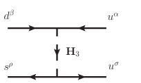
Figure 1: Tree diagram for the $K\to\pi\pi$ decays mediated by color-triplet diquark ${\bf H}_{3}$.

Using the Yukawa couplings in Eq. (11), the four-fermion interactions can be written as:

$${\cal H}_{\rm tree} =-\frac{1}{2m^{2}_{H_{3}}}\left[g^{L}_{11}g^{L*}_{12}(\overline{u^{C\alpha}}P_{L}d^{\beta})\,(\bar{s}_{\beta}P_{R}u^{C}_{\alpha})+g^{R}_{11}g^{R*}_{12}(\overline{u^{C\alpha}}P_{R}d^{\beta})\,(\bar{s}_{\beta}P_{L}u^{C}_{\alpha})\right.$$

$$\left.+g^{L}_{11}g^{R*}_{12}(\overline{u^{C\alpha}}P_{L}d^{\beta})\,(\bar{s}_{\beta}P_{L}u^{C}_{\alpha})+g^{R}_{11}g^{L*}_{12}(\overline{u^{C\alpha}}P_{R}d^{\beta})\,(\bar{s}_{\beta}P_{R}u^{C}_{\alpha})\right]\,,$$ (24)

where the charge-conjugation state of a fermion is defined by $f^{C}=C\gamma_{0}f^{*}=C\bar{f}^{T}$. We can express the ${\cal H}_{\rm tree}$ in terms of fermion states using the Fierz and $C$-parity transformations, which are:

$$\bar{f}_{3}P_{\chi}f_{2}\,\bar{f}_{1}P_{\chi}f_{4} =-\frac{1}{2}(\bar{f}_{2}P_{\chi}f_{1})(\bar{f}_{3}P_{\chi}f_{4})-\frac{1}{8}(\bar{f}_{2}\sigma_{\mu\nu}P_{\chi}f_{1})(\bar{f}_{3}\sigma^{\mu\nu}P_{\chi}f_{4})\,,$$

$$\overline{f^{C}}P_{\chi}f^{C} =\bar{f}P_{\chi}f\,,$$

$$\overline{f^{C}}\sigma_{\mu\nu}P_{\chi}f^{C} =-\bar{f}\sigma_{\mu\nu}P_{\chi}f\,,$$ (25)

with $P_{\chi}=P_{R(L)}$. As a result, Eq. (24) can be formulated as:

$${\cal H}_{\rm tree} =-\frac{G_{F}V^{*}_{ts}V_{td}}{\sqrt{2}}\frac{y_{W}}{2}\left[\zeta^{LL}_{21}\left(Q_{1}-Q_{2}\right)+\zeta^{RR}_{21}\left(Q^{\prime}_{1}-Q^{\prime}_{2}\right)\right.$$

$$-\zeta^{LR}_{21}\left(4\left(Q^{SLL,u}_{1}+Q^{SLL,u}_{2}\right)+Q^{SLL,u}_{3}+Q^{SLL,u}_{4}\right)$$

$$\left.-\zeta^{RL}_{21}\left(4\left(Q^{\prime SLL,u}_{1}+Q^{\prime SLL,u}_{2}\right)+Q^{\prime SLL,u}_{3}+Q^{\prime SLL,u}_{4}\right)\right]\,,$$ (26)

where $G_{F}$ is the Fermi constant; $V_{ij}$ denotes the CKM matrix element; $y_{W}=m^{2}_{W}/m^{2}_{H_{3}}$, and the parameters $\zeta^{\chi}_{21}$ are defined as:

$$\zeta^{LL(RR)}_{21}=\frac{g^{L(R)}_{11}g^{L(R)*}_{12}}{g^{2}V^{*}_{ts}V_{td}}\,,~{}\zeta^{LR(RL)}_{21}=\frac{g^{L(R)}_{11}g^{R(L)*}_{12}}{g^{2}V^{*}_{ts}V_{td}}\,.$$ (27)

Following the notations shown in Buras:2000if ; Aebischer:2018rrz , the effective operators are defined as:

$$Q_{1} =(\bar{s}d)_{V-A}(\bar{u}u)_{V-A}\,,~{}Q_{2}=(\bar{s}u)_{V-A}(\bar{u}d)_{V-A}\,,$$

$$Q^{SLL,u}_{1} =(\bar{s}_{\alpha}P_{L}u^{\beta})(\bar{u}_{\beta}P_{L}d^{\alpha})\,,~{}Q^{SLL,u}_{2}=(\bar{s}_{\alpha}P_{L}d^{\alpha})(\bar{u}_{\beta}P_{L}u^{\beta})\,,$$

$$Q^{SLL,u}_{3} =-(\bar{s}_{\alpha}\sigma_{\mu\nu}P_{L}u^{\beta})(\bar{u}_{\beta}\sigma^{\mu\nu}P_{L}d^{\alpha})\,,~{}Q^{SLL,u}_{4}=-(\bar{s}_{\alpha}\sigma_{\mu\nu}P_{L}d^{\alpha})(\bar{u}_{\beta}\sigma^{\mu\nu}P_{L}u^{\beta})\,,$$ (28)

where $(\bar{f}f)_{V-A}=\bar{f}\gamma_{\mu}(1-\gamma_{5})f$, and the prime operators can be obtained from unprimed ones using $P_{L(R)}$ instead of $P_{R(L)}$. It can be seen that the current-current interactions induced at the tree-level involve vector-, scalar-, and tensor-type currents. Although the tensor-tensor operator contributions to the $K\to\pi\pi$ decays vanish at the factorization scale, since a large mixing between the scalar-scalar and tensor-tensor operators is induced at one-loop QCD corrections Aebischer:2018rrz , the tensor-type interaction can have a large contribution to $\epsilon^{\prime}/\epsilon$.

III.1.2 QCD penguins

In addition to the tree-level diagrams, the $K\to\pi\pi$ decays in the diquark model can arise from the gluon-penguin diagrams, as shown in Fig. 2. As is known, the loop diagram usually leads to an ultraviolet divergence. To obtain the finite coupling for the $d\to sg^{(*)}$ vertex, we have to renormalize the three-point vertex function by including the self-energy diagram for the $d\to s$ flavor changing transition. The detailed discussions for renormalizing the $d\to sg^{(*)}$ vertex are given in the appendix; here, we simply use the obtained results of Fig. 2(a) and (b) to produce the effective Hamiltonian for the $K\to\pi\pi$ decays.

Figure 2: Gluon-penguin diagrams for the $d\to sg^{(*)}$ transition mediated by color-triplet diquark ${\bf H}_{3}$.

Because the gluon momentum $k$ satisfies $k^{2}\ll m^{2}_{t},m^{2}_{H_{3}}$, we can expand the three-point functions in terms of $k^{2}/m^{2}_{H_{3}}$ and keep the leading $k^{2}/m^{2}_{H_{3}}$ terms. Thus, based on the renormalized vertex obtained in Eq. (128), the penguin-induced Lagrangian for $d\to sg^{*}$ can be expressed as:

$${\cal L}_{d\to sg^{*}}=-\frac{g_{s}\,k^{2}}{(4\pi)^{2}m^{2}_{H_{3}}}I_{G1}(y_{t})\bar{s}\gamma^{\mu}\left(g^{L}_{31}g^{L*}_{32}P_{L}+g^{R}_{31}g^{R*}_{32}P_{R}\right)T^{a}d\,A^{a}_{\mu}\,,$$ (29)

where $I_{G1}(y_{t})$ with $y_{t}=m^{2}_{t}/m^{2}_{H_{3}}$ denotes the loop integral function and can be found from Eq. (129). The $k^{2}$ factor in the numerator can be used to cancel the off-shell gluon propagator, i.e., $1/(k^{2}+i\varepsilon)$. Accordingly, the effective Hamiltonian for the $d\to s\bar{q}q$ decays from the gluon-penguin can be obtained as:

$${\cal H}_{\rm QCD} =-\frac{\alpha_{s}I_{G1}(y_{t})}{32\pi m^{2}_{H_{3}}}\left[g^{L*}_{32}g^{L}_{31}\left(Q_{4}+Q_{6}-\frac{1}{3}Q_{3}-\frac{1}{3}Q_{5}\right)\right.$$

$$\left.+g^{R*}_{32}g^{R}_{31}\left(Q^{\prime}_{4}+Q^{\prime}_{6}\ -\frac{1}{3}Q^{\prime}_{3}-\frac{1}{3}Q^{\prime}_{5}\right)\right]\,,$$ (30)

where we have used:

$$(T^{a})^{\alpha}_{\beta}(T^{a})^{\rho}_{\sigma}=\frac{1}{2}\left(\delta^{\alpha}_{\sigma}\delta^{\rho}_{\beta}-\frac{1}{3}\delta^{\alpha}_{\beta}\delta^{\rho}_{\sigma}\right)\,;$$ (31)

the unprimed operators at the $m_{H_{3}}$ scale are the same as those in the SM and can be found as:

$$Q_{3} =(\bar{s}d)_{V-A}\sum_{q}(\bar{q}q)_{V-A}\,,~{}Q_{4}=(\bar{s}_{\alpha}d^{\beta})_{V-A}\sum_{q}(\bar{q}_{\alpha}q^{\beta})_{V-A}\,,$$

$$Q_{5} =(\bar{s}d)_{V-A}\sum_{q}(\bar{q}q)_{V+A}\,,~{}Q_{6}=(\bar{s}_{\alpha}d^{\beta})_{V-A}\sum_{q}(\bar{q}_{\alpha}q^{\beta})_{V+A}\,,$$ (32)

and the prime operators can be obtained from the unprimed ones via the exchange of $P_{L(R)}$ and $P_{R(L)}$.

III.1.3 EW penguins

The $d\to sq\bar{q}$ decays can be also induced from the EW penguin diagrams through the mediation of the off-shell photon and $Z$-boson, where the Feynman diagrams are shown in Fig. 3. Similar to the case in $d\to sg^{(*)}$, there are ultraviolet divergences in the loop integrals of Fig. 3(a) and (b). The discussions for the divergence cancellation are given in the appendix. According to Eqs. (136) and (146), the loop-induced Lagrangian for $d\to s(\gamma^{*},Z^{*})$ can be written as:

$${\cal L}_{s\to d\gamma^{*},Z^{*}} =-\frac{ek^{2}}{3(4\pi)^{2}m^{2}_{H_{3}}}I_{\gamma 1}(y_{t})\bar{s}\gamma^{\mu}\left(g^{L}_{31}g^{L*}_{32}P_{L}+g^{R}_{31}g^{R*}_{32}P_{R}\right)d\,A_{\mu}\,,$$

$$-\frac{g}{2\cos\theta_{W}(4\pi)^{2}}\bar{s}\gamma^{\mu}I_{Z}(y_{t})\left(g^{L}_{31}g^{L*}_{32}P_{L}-g^{R}_{31}g^{R*}_{32}P_{R}\right)d\,Z_{\mu}\,,$$ (33)

where $I_{\gamma 1}$ and $I_{Z}$ are the associated loop functions and can be found in Eqs. (137) and (147).

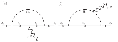
Figure 3: Feynman diagrams for the $d\to s(\gamma^{(*)}\,,Z^{*})$ processes.

Based on Eq. (33), the effective Hamiltonian for the $d\to sq\bar{q}$ decays can be written as:

$${\cal H}_{EW}=-\frac{G_{F}V^{*}_{ts}V_{td}}{\sqrt{2}}\left[C^{Z}_{3}Q_{3}+C^{\prime Z}_{5}Q^{\prime}_{5}+\sum^{10}_{i=7}\left(C^{\gamma Z}_{i}Q_{i}+C^{\prime\gamma Z}_{i}Q^{\prime}_{i}\right)\right]\,,$$ (34)

where the effective operators $Q_{7}$-$Q_{10}$ are the same as those in the SM and are expressed as:

$$Q_{7} =\frac{3}{2}(\bar{s}d)_{V-A}\sum_{q}e_{q}(\bar{q}q)_{V+A}\,,\ Q_{8}=\frac{3}{2}(\bar{s}_{\alpha}d^{\beta})_{V-A}\sum_{q}e_{q}(\bar{q}_{\beta}q^{\alpha})_{V+A}\,,$$

$$Q_{9} =\frac{3}{2}(\bar{s}d)_{V-A}\sum_{q}e_{q}(\bar{q}q)_{V-A}\,,\ Q_{10}=\frac{3}{2}(\bar{s}_{\alpha}d^{\beta})_{V-A}\sum_{q}e_{q}(\bar{q}_{\beta}q^{\alpha})_{V-A}\,,$$ (35)

and $e_{q}$ is the $q$-quark electric charge. The prime operators $Q^{\prime}_{7}$-$Q^{\prime}_{10}$ can be obtained from the unprimed operators through the exchange of $P_{L(R)}$ and $P_{R(L)}$. The effective Wilson coefficients $C^{(\prime)Z}_{i}$ and $C^{(\prime)\gamma Z}_{i}$ are given as:

$$C^{Z}_{3} =\frac{\alpha}{6\pi\sin^{2}\theta_{W}}\frac{I_{Z}(y_{t})h^{L}_{21}}{4}\,,~{}C^{\prime Z}_{5}=-\frac{\alpha}{6\pi\sin^{2}\theta_{W}}\frac{I_{Z}(y_{t})h^{R}_{21}}{4}\,,$$

$$C^{\gamma Z}_{7} =\frac{4\alpha}{6\pi}\frac{I_{Z}(y_{t})h^{L}_{21}}{4}+\frac{\alpha}{6\pi}\frac{2y_{W}I_{\gamma 1}(y_{t})h^{L}_{21}}{3}\,,~{}C^{\gamma Z}_{9}=C^{\gamma Z}_{7}-4C^{Z}_{3}\,,$$

$$C^{\prime\gamma Z}_{9} =-\frac{4\alpha}{6\pi}\frac{I_{Z}(y_{t})h^{R}_{21}}{4}+\frac{\alpha}{6\pi}\frac{2y_{W}I_{\gamma 1}(y_{t})h^{R}_{21}}{3}\,,~{}C^{\prime\gamma Z}_{7}=C^{\prime\gamma Z}_{9}-4C^{\prime Z}_{5}\,,$$ (36)

where $\alpha=e^{2}/4\pi$; $y_{W}=m^{2}_{W}/m^{2}_{H_{3}}$; $C^{(\prime)\gamma Z}_{8}=C^{(\prime)\gamma Z}_{10}=0$, and the $h^{L,R}_{21}$ parameters are defined by:

$$h^{L}_{21}=\frac{g^{L*}_{32}g^{L}_{31}}{g^{2}V^{*}_{ts}V_{td}}\,,~{}h^{R}_{21}=\frac{g^{R*}_{32}g^{R}_{31}}{g^{2}V^{*}_{ts}V_{td}}\,.$$ (37)

We can use the new parameters $h^{L,R}_{21}$ to study the diquark contributions to $\epsilon^{\prime}/\epsilon$.

III.1.4 Combination of the QCD and EW penguins and CMOs

After respectively obtaining the QCD and EW penguin contributions to the $d\to sq\bar{q}$ decays, the effective Hamiltonian for the $\Delta S=1$ processes in the diquark model can be combined as:

$${\cal H}_{\Delta S=1}=-\frac{G_{F}V^{*}_{ts}V_{td}}{\sqrt{2}}\sum_{i=3}^{10}\left(y^{H_{3}}_{i}Q_{i}+y^{\prime H_{3}}_{i}Q^{\prime}_{i}\right)\,,$$ (38)

where the effective Wilson coefficients $y^{H_{3}}_{i}$ and $y^{\prime H_{3}}_{i}$ are given as:

$$y^{H_{3}}_{3} =-\frac{\alpha_{s}}{12\pi}h^{L}_{21}y_{W}I_{G1}(y_{t})+C^{Z}_{3}\,,~{}y^{H_{3}}_{4}=\frac{\alpha_{s}}{4\pi}h^{L}_{21}y_{W}I_{G1}(y_{t})\,,$$

$$y^{H_{3}}_{5} =-\frac{\alpha_{s}}{12\pi}h^{L}_{21}y_{W}I_{G1}(y_{t})\,,~{}y^{H_{3}}_{6}=y^{H_{3}}_{4}\,,~{}y^{H_{3}}_{7}=C^{\gamma Z}_{7}\,,~{}y^{H_{3}}_{9}=C^{\gamma Z}_{9}\,,$$

$$y^{\prime H_{3}}_{3} =-\frac{\alpha_{s}}{12\pi}h^{R}_{21}y_{W}I_{G1}(y_{t})\,,~{}y^{\prime H_{3}}_{4}=\frac{\alpha_{s}}{4\pi}h^{R}_{21}y_{W}I_{G1}(y_{t})\,,$$

$$y^{\prime H_{3}}_{5} =y^{\prime H_{3}}_{3}+C^{\prime Z}_{5}\,,~{}y^{\prime H_{3}}_{6}=y^{\prime H_{3}}_{4}\,,~{}y^{\prime H_{3}}_{7}=C^{\prime\gamma Z}_{7}\,,~{}y^{\prime H_{3}}_{9}=C^{\prime\gamma Z}_{9}\,,$$ (39)

and $y^{H_{3}}_{8,10}=y^{\prime H_{3}}_{8,10}=0$. Hence, we will use Eqs. (38) and (39) to study $\epsilon^{\prime}/\epsilon$.

In addition to the QCD and EW penguins, the gluonic and electromagnetic dipole operators can contribute to the $K\to\pi\pi$ decays. Since the strong interactions dominate, we only study the gluonic dipole contributions in this paper. Therefore, according to Eq. (128), the effective Hamiltonian for $d\to sg$ in the chromomagnetic dipole form can be written as:

$${\cal H}_{d\to sg}=-\frac{G_{F}V^{*}_{ts}V_{td}}{\sqrt{2}}\left(C^{H_{3}}_{8G}Q_{8G}+C^{\prime H_{3}}_{8G}Q^{\prime}_{8G}\right)\,,$$ (40)

where the dimension-6 CMOs $Q^{(\prime)}_{8G}$ are defined as:

$$Q_{8G} =\frac{g_{s}}{8\pi^{2}}m_{s}\bar{s}\sigma\cdot GP_{L}d\,,$$

$$Q^{\prime}_{8G} =\frac{g_{s}}{8\pi^{2}}m_{d}\bar{s}\sigma\cdot GP_{R}d\,,$$ (41)

with $\sigma\cdot G=\sigma^{\mu\nu}T^{a}G^{a}_{\mu\nu}$, and the associated Wilson coefficients are shown as:

$$C^{H_{3}}_{8G}=\frac{m_{t}}{m_{s}}\frac{g^{R*}_{32}}{g^{L*}_{32}}h^{L}_{21}y_{W}I_{G2}(y_{t})\,,~{}C^{\prime H_{3}}_{8G}=\frac{m_{t}}{m_{d}}\frac{g^{L*}_{32}}{g^{R*}_{32}}h^{R}_{21}y_{W}I_{G2}(y_{t})\,.$$ (42)

$I_{G2}$ is the loop integral function and can be found from Eq. (129). Because the involved ${\bf H}_{3}$ Yukawa couplings in the induced CMOs are $g^{R*}_{32}g^{L}_{31}$ and $g^{L*}_{32}g^{R}_{31}$, from Eq. (42), it is seen that $h^{L}_{21}$ and $h^{R}_{21}$ are associated with $g^{R*}_{32}/g^{L*}_{32}$ and $g^{L*}_{32}/g^{R*}_{32}$ factors, respectively. Since $g^{R}_{32}$ and $g^{L}_{32}$ cannot be singly constrained, we can take $g^{R}_{32}/g^{L}_{32}\approx 1$ and just use $h^{L,R}_{21}$ as the independent variables to study the CMO effects. Recently, the $K\to\pi\pi$ matrix elements of the CMOs were calculated based on a DQCD approach Buras:2018evv , and the results are consistent with the lattice QCD, as calculated by ETM collaboration Constantinou:2017sgv . We use the Hamiltonian in Eq. (40) and the $K\to\pi\pi$ matrix elements obtained using the DQCD approach to investigate the CMO effects on $\epsilon^{\prime}/\epsilon$.

III.2 $\Delta S=2$ in the diquark model

Next, we study the ${\bf H}_{3}$ contributions to the $\Delta S=2$ process, where the involved Feynman diagrams are sketched in Fig. 4. It has been pointed out that the contribution of Fig. 4(a) vanishes in the chiral limit, i.e., $m_{t}\sim 0$ Barr:1989fi . In the following analysis, in addition to discussing the origin of the vanished result, we also demonstrate that the Fig. 4(a) contribution is interesting and important when $m_{t}\approx 165$ GeV and $m_{H_{3}}\approx{\cal O}$(1) TeV are taken.

Figure 4: Box diagrams for $\Delta S=2$ in the diquark model, where the subscripts denote the color indices.

To study the diquark contributions to $\Delta S=2$, we follow the notations in Buras:2001ra and write the effective Hamiltonian as:

$${\cal H}_{\Delta S=2}=\frac{G^{2}_{F}V_{\rm CKM}}{16\pi^{2}}m^{2}_{W}\sum_{i}C^{\chi}_{i}(\mu)Q^{\chi}_{i}\,,$$ (43)

where $V_{\rm CKM}=(V^{*}_{ts}V_{td})^{2}$ is the product of the CKM matrix elements; $C^{\chi}_{i}(\mu)$ are the Wilson coefficients at the $\mu$ scale, and the relevant operators $Q^{\chi}_{i}$ are given as:

$$Q^{VLL}_{1} =(\bar{s}\gamma_{\mu}P_{L}d)(\bar{s}\gamma^{\mu}P_{L}d)\,,$$

$$Q^{LR}_{1} =(\bar{s}\gamma_{\mu}P_{L}d)(\bar{s}\gamma^{\mu}P_{R}d)\,,$$

$$Q^{LR}_{2} =(\bar{s}P_{L}d)(\bar{s}P_{R}d)\,,$$

$$Q^{SLL}_{1} =(\bar{s}P_{L}d)(\bar{s}P_{L}d)\,,$$

$$Q^{SLL}_{2} =(\bar{s}\sigma_{\mu\nu}P_{L}d)(\bar{s}\sigma^{\mu\nu}P_{L}d).$$ (44)

The operators $Q^{VRR}_{1}$ and $Q^{SRR}_{i}$ can be obtained from $Q^{VLL}_{1}$ and $Q^{SLL}_{i}$ by switching $P_{R}$ and $P_{L}$, respectively. We use the effective operators in Eq. (44) to show the diquark contributions.

III.2.1 Box diagrams with one $W$-boson and one diquark

Based on the Yukawa couplings in Eq. (11) and using the ’t Hooft-Feynman gauge, the effective Hamiltonian for $\Delta S=2$ via the mediation of $W$ and ${\bf H}_{3}$ shown in Fig. 4(a) can be written as:

$${\cal H}^{WH_{3}}_{\Delta S=2} =-\frac{g^{2}V^{*}_{ts}V_{td}}{2}(\bar{K}_{a})_{\rho\beta}(K^{a})^{\rho^{\prime}\beta^{\prime}}\int\frac{d^{4}q}{(2\pi)^{4})}\frac{1}{(q^{2}-m^{2}_{H^{2}_{3}})(q^{2}-m^{2}_{W})(q^{2}-m^{2}_{t})^{2}}$$

$$\times\left[g^{L}_{31}g^{L*}_{32}\left(\overline{d^{C\rho}}\not{q}\gamma_{\mu}P_{L}d^{\beta}\right)\left(\bar{s}_{\rho^{\prime}}\gamma^{\mu}\not{q}P_{R}s^{C}_{\beta^{\prime}}\right)+m^{2}_{t}g^{R}_{31}g^{R*}_{32}\left(\overline{d^{C\rho}}\gamma_{\mu}P_{L}d^{\beta}\right)\left(\bar{s}_{\rho^{\prime}}\gamma^{\mu}P_{L}s^{C}_{\beta^{\prime}}\right)\right]\,,$$ (45)

It can be seen that because $W$-boson only couples to the left-handed quarks, without the chirality flipping effect, e.g. $m_{t}$, the first term depends on $g^{L}_{31}g^{L*}_{32}$. With the chirality flip, which arises from the mass insertions in the two top-quark propagators, the second term in Eq. (45) is associated with the right-handed quark couplings $m^{2}_{t}g^{R}_{31}g^{R*}_{32}$.

Although $g^{L}_{31}g^{L*}_{32}$ appears in Eq. (45), we demonstrate that its contribution indeed vanishes when the color factor and Fierz transformation are considered together. Using $\gamma_{\mu}\gamma_{\nu}=g_{\mu\nu}-i\sigma_{\mu\nu}$ and Fierz transformation, the first term in Eq. (45) can be derived as:

$$\left(\overline{d^{C\rho}}\gamma_{\nu}\gamma_{\mu}P_{L}d^{\beta}\right)\left(\bar{s}_{\rho^{\prime}}\gamma^{\mu}\gamma^{\nu}P_{R}s^{C}_{\beta^{\prime}}\right) =-2\left(\overline{d^{C\rho}}\gamma_{\mu}P_{R}s^{C}_{\beta^{\prime}}\right)\left(\bar{s}_{\rho^{\prime}}\gamma^{\mu}P_{L}d^{\beta}\right)$$

$$=2\bar{s}_{\beta^{\prime}}\gamma_{\mu}P_{L}d^{\rho}\bar{s}_{\rho^{\prime}}\gamma^{\mu}P_{L}d^{\beta}\,.$$ (46)

We note that because the chirality of initial quark can not match with that of final quark, the tensor-type current is not allowed. Combined with the color factor $(\bar{K}_{a})_{\rho\beta}(K^{a})^{\rho^{\prime}\beta^{\prime}}=(\delta^{\beta^{\prime}}_{\rho}\delta^{\rho^{\prime}}_{\beta}-\delta^{\rho^{\prime}}_{\rho}\delta^{\beta^{\prime}}_{\beta})/2$, the result of above equation can be proceeded as:

$$2(\bar{K}_{a})_{\rho\beta}(K^{a})^{\rho^{\prime}\beta^{\prime}}\bar{s}_{\beta^{\prime}}\gamma_{\mu}P_{L}d^{\rho}\bar{s}_{\rho^{\prime}}\gamma^{\mu}P_{L}d^{\beta}=\bar{s}\gamma_{\mu}P_{L}d\bar{s}\gamma^{\mu}P_{L}d-\bar{s}_{\beta}\gamma_{\mu}P_{L}d^{\rho}\bar{s}_{\rho}\gamma^{\mu}P_{L}d^{\beta}=0.$$ (47)

The vanished result is from the cancellation between the first and second term when the Fierz transformation is applied to the second term. Clearly, in the limit of $m_{t}\sim 0$, the box diagrams mediated by one $W$ and one ${\bf H}_{3}$ have no contributions to the $\Delta S=2$ process. Hence, the nonvanished ${\cal H}^{WH_{3}}_{\Delta S=2}$ is from the $g^{R}_{31}g^{R*}_{32}$ term. In order to avoid the gauge dependence, we have to include the charged-Goldstone-boson contributions, where the dominant Yukawa coupling is $m_{t}V_{tq}/(\sqrt{2}m_{W})\,\bar{t}_{R}q_{L}G^{+}$ (q=d,s). In terms of the effective operators in Eq. (44), we can write the effective Hamiltonian to be:

$${\cal H}^{WH_{3}}_{\Delta S=2}=\frac{G^{2}_{F}V_{\rm CKM}}{16\pi^{2}}m^{2}_{W}\left(C^{LR}_{WH_{3},1}Q^{LR}_{1}+C^{LR}_{WH_{3},2}Q^{LR}_{2}\right)\,,$$ (48)

where the effective Wilson coefficients are given as:

$$C^{LR}_{WH_{3},1} =4h^{R}_{21}\left[y_{W}I^{WH_{3}}_{\rm Box}(y_{W},y_{t})-I^{GH_{3}}_{\rm Box}(y_{W},y_{t})\right]\,,~{}C^{LR}_{WH_{3},2}=2C^{LR}_{WH_{3},1}\,,$$

$$I^{WH_{3}}_{\rm Box}(y_{W},y_{t}) =\frac{y_{t}}{(y_{t}-y_{W})^{2}}\left[\frac{y_{t}-y_{W}}{1-y_{t}}+\frac{y_{W}\ln y_{W}}{1-y_{W}}+\frac{(y^{2}_{t}-y_{W})\ln y_{t}}{(1-y_{t})^{2}}\right]\,,$$

$$I^{GH_{3}}_{\rm Box}(y_{W},y_{t}) =-\frac{y^{2}_{t}}{2(1-y_{t})(y_{t}-y_{W})}-\frac{y_{t}y^{2}_{W}\ln y_{W}}{2(1-y_{W})(y_{t}-y_{W})^{2}}$$

$$-\frac{y^{2}_{t}\left(y_{t}-(2-y_{t})y_{W}\right)\ln y_{t}}{2(1-y_{t})^{2}(y_{t}-y_{W})^{2}}\,.$$ (49)

With $m_{H_{3}}=1.5$ TeV, the loop functions can be $I^{WH_{3}}_{\rm Box}(y_{W},y_{t})\approx 0.68$ and $I^{GH_{3}}(y_{W},y_{t})\approx 0.02$. However, when $y_{W}$ factor is included, we obtain $y_{W}I^{WH_{3}}_{\rm Box}(y_{W},y_{t})\approx 0.002$, which is smaller than $I^{GH_{3}}_{\rm Box}(y_{W},y_{t})$ by one order of magnitude; that is, $I^{GH_{3}}_{\rm Box}$ dominates.

III.2.2 Box diagrams from the color-triplet diquark

The effective Hamiltonian through the mediation of the diquark ${\bf H}_{3}$ shown in Fig. 4(b) can be written as:

$$-i{\cal H}^{H_{3}}_{\Delta S=2} =\frac{K_{C}}{2}\int\frac{d^{4}q}{(2\pi)^{4}}\frac{{\cal N}_{H_{3}}}{(q^{2}-m^{2}_{W})^{2}(q^{2}-m^{2}_{t})^{2}}\,,$$ (50)

$$K_{C} =(\bar{K}_{b})_{\beta\alpha}(K^{b})^{\alpha^{\prime}\rho^{\prime}}(\bar{K}_{a})_{\beta^{\prime}\alpha^{\prime}}(K^{a})^{\alpha\rho}=\frac{1}{4}\left(\delta^{\rho}_{\beta^{\prime}}\delta^{\rho^{\prime}}_{\beta}+\delta^{\rho^{\prime}}_{\beta^{\prime}}\delta^{\rho}_{\beta}\right)\,,$$

$${\cal N}_{H_{3}} =(\bar{s}_{\rho}\not{q}\chi^{V}_{21}d^{\beta})(\bar{s}_{\rho^{\prime}}\not{q}\chi^{V}_{21}d^{\beta^{\prime}})+m^{2}_{t}(\bar{s}_{\rho}\chi^{S}_{21}d^{\beta})(\bar{s}_{\rho^{\prime}}\chi^{S}_{21}d^{\beta^{\prime}})\,,$$ (51)

where the crossed diagram by exchanging top-quark and ${\bf H}_{3}$ is included, and the definitions of $\chi^{V}_{21}$ and $\chi^{S}_{21}$ can be found from Eq. (113) in the appendix. Using the Fierz transformations and the identities in Eq. (25), we find that the effective operators in Eq. (44) can be all generated from the box diagrams, and Eq. (50) can be formed as:

$${\cal H}^{H_{3}}_{\Delta S=2} =\frac{G^{2}_{F}V_{\rm CKM}}{16\pi^{2}}m^{2}_{W}\left[C^{VLL}_{H_{3},1}Q^{VLL}_{1}+C^{VRR}_{H_{3},1}Q^{VRR}_{1}+C^{LR}_{H_{3},1}Q^{LR}_{1}+C^{LR}_{H_{3},2}Q^{LR}_{2}\right.$$

$$\left.+C^{SLL}_{H_{3},1}Q^{SLL}_{1}+C^{SLL}_{H_{3},2}Q^{SLL}_{2}+C^{SRR}_{H_{3},1}Q^{SRR}_{1}+C^{SRR}_{H_{3},2}Q^{SRR}_{2}\right]\,,$$ (52)

where the associated effective Wilson coefficients at the $\mu=m_{H_{3}}$ scale are expressed as:

$$C^{VLL}_{H_{3},1} =4y_{W}I^{H_{3}}_{B1}(y_{t})\left(h^{L}_{21}\right)^{2}\,,~{}C^{VRR}_{H_{3},1}=4y_{W}I^{H_{3}}_{B1}(y_{t})\left(h^{R}_{21}\right)^{2}\,,$$

$$C^{LR}_{H_{3},1} =4y_{W}\left[I^{H_{3}}_{B1}(y_{t})+I^{H_{3}}_{B2}(y_{t})\right]h^{L}_{21}h^{R}_{21}\,,~{}C^{LR}_{H_{3},2}=-2C^{LR}_{H_{3},1}\,,$$

$$C^{SLL}_{H_{3},1} =2y_{W}I^{H_{3}}_{B2}(y_{t})(h^{L}_{21})^{2}\,,~{}C^{SLL}_{H_{3},2}=-\frac{C^{SLL}_{H_{3},1}}{4}\,,$$

$$C^{SRR}_{H_{3},1} =2y_{W}I^{H_{3}}_{B2}(y_{t})(h^{R}_{21})^{2}\,,~{}C^{SRR}_{H_{3},2}=-\frac{C^{SRR}_{H_{3},1}}{4}\,.$$ (53)

The loop functions $I^{H_{3}}_{B1}(y_{t})$ and $I^{H_{3}}_{B2}(y_{t})$ are defined as:

$$I^{H_{3}}_{B1}(y) =\frac{1+y}{2(1-y)^{2}}+\frac{y\ln y}{(1-y)^{3}}\,,$$

$$I^{H_{3}}_{B2}(y) =-\frac{2y}{(1-y)^{2}}-\frac{y(1+y)\ln y}{(1-y)^{3}}\,.$$ (54)

From the interactions in Eq. (52), it can be seen that eight different operators are involved. We will show that although the hadronic matrix elements of $Q^{VLL}_{1}$ and $Q^{VRR}_{1}$ are smaller than those of $Q^{SLL}_{i}$ and $Q^{SRR}_{i}$, due to $I^{H_{3}}_{B2}(y_{t})\ll I^{H_{3}}_{B1}(y_{t})$, their contributions indeed are comparable.

IV $\epsilon^{\prime}/\epsilon$ and $\epsilon_{K}$ with hadronic effects in the diquark model

IV.1 Matrix elements for the $K\to\pi\pi$ decays

The decay amplitudes for $K\to\pi\pi$ in terms of the isospin of $\pi\pi$ final state can be written as Cirigliano:2011ny :

$$A(K^{+}\to\pi^{+}\pi^{0}) =\frac{3}{2}A_{2}e^{i\delta_{2}}\,,$$

$$A(K^{0}\to\pi^{+}\pi^{-}) =A_{0}e^{i\delta_{0}}+\sqrt{\frac{1}{2}}A_{2}e^{i\delta_{2}}\,,$$

$$A(K^{0}\to\pi^{0}\pi^{0}) =A_{0}e^{i\delta_{0}}-\sqrt{2}A_{2}e^{i\delta_{2}}\,$$ (55)

where $A_{0(2)}$ denotes the isospin $I=0(2)$ amplitude; $\delta_{0(2)}$ is the strong phase and $\delta_{0}-\delta_{2}=(47.5\pm 0.9)^{\circ}$ Cirigliano:2011ny . The experimental data indicate $ReA^{\rm exp}_{0}=27.04(1)\times 10^{-8}$ GeV and $ReA^{\rm exp}_{2}=1.210(2)\times 10^{-8}$ GeV PDG . Using the isospin amplitudes, the direct CP violating parameter from new physics in $K$ system can be estimated by Buras:2015yba :

$$Re\left(\frac{\epsilon^{\prime}}{\epsilon}\right)\approx-\frac{\omega}{\sqrt{2}|\epsilon_{K}|}\left[\frac{ImA_{0}}{ReA_{0}}-\frac{ImA_{2}}{ReA_{2}}\right]\,,$$ (56)

where $\omega=ReA_{2}/ReA_{0}\approx 1/22.35$ denotes the $\Delta I=1/2$ rule. From Eq. (56), it is seen that $\epsilon^{\prime}/\epsilon$ is related to the ratios of hadronic matrix elements. In the following, we summarize the relevant matrix elements for the involved operators that are from the tree-level and loop diagrams.

IV.1.1 $K\to\pi\pi$ hadronic matrix elements of the tree-level operators

Although only one Feynman diagram is used to generate the $\Delta S=1$ processes at the tree level, from Eq. (26), twelve effective operators are involved in the processes, such as $Q_{1,2}$, $Q^{SLL,u}_{1-4}$ and their prime operators. The operators $Q_{1,2}$ are the same as those generated via the mediation of $W$-boson in the SM; thus, the associated hadronic matrix elements can be quoted from the SM calculations. However, the operators $Q^{SLL,u}_{i}$ are new operators and do not mix with the SM operators; therefore, if $Q_{1,2}$ and $Q^{SLL,u}$ are taken as two different classes of operators, we can separately introduce their matrix elements. According to the notations in Buras:2015yba , we thus define the new operators in terms of $Q_{1}$ and $Q_{2}$ as:

$$Q_{+}=\frac{1}{2}\left(Q_{2}+Q_{1}\right)\,,~{}Q_{-}=\frac{1}{2}\left(Q_{2}-Q_{1}\right)\,.$$ (57)

The isospin amplitudes for the $K\to\pi\pi$ decays in the SM can be given as Buras:2015yba :

$$ReA^{\rm SM}_{0} \approx\frac{G_{F}V^{*}_{us}V_{ud}}{\sqrt{2}}z_{-}\langle Q_{-}\rangle_{0}\left(1+q_{T}\right)\,,$$

$$ReA^{\rm SM}_{2} \approx\frac{G_{F}V^{*}_{us}V_{ud}}{\sqrt{2}}z_{+}\langle Q_{+}\rangle_{2}\,.$$ (58)

where $q_{T}=z_{+}\langle Q_{+}\rangle_{0}/(z_{-}\langle Q_{-}\rangle_{0})$, $z_{\pm}=z_{2}\pm z_{1}$, and the values of $z_{1,2}$ at $\mu=m_{c}$ are $z_{1}=-0.409$ and $z_{2}=1.212$ Buras:2015yba . Because $q_{T}\lesssim 0.1$, we will ignore its contribution in the new physics study. In addition, we assume $ReA^{\rm SM}_{0(2)}\approx ReA^{\rm exp}_{0(2)}$ in the following analysis; that is, $\langle Q_{\pm}\rangle$ can be determined by the experimental data.

Using the results obtained in Aebischer:2018rrz , the matrix elements arisen from the $Q^{SLL,u}_{i}$ operators for the isospin $I=0$ at the factorizable scale are given as:

$$\langle Q^{SLL,u}_{1}\rangle_{0} =\frac{r^{2}(\mu)}{48}f_{\pi}\,,~{}\langle Q^{SLL,u}_{2}\rangle_{0}=-\frac{r^{2}(\mu)}{24}f_{\pi}\,,$$

$$\langle Q^{SLL,u}_{3}\rangle_{0} =-\frac{r^{2}(\mu)}{4}f_{\pi}\,,~{}\langle Q^{SLL,u}_{4}\rangle_{0}=0\,,$$ (59)

with

$$r(\mu)=\frac{2m^{2}_{K}}{m_{s}(\mu)+m_{d}(\mu)}\,.$$ (60)

The matrix elements for the isospin $I=2$ are given as $\langle O^{SLL,u}_{i}\rangle_{2}=\langle O^{SLL,u}_{i}\rangle_{0}/\sqrt{2}$. Based on the DQCD approach, the matrix elements at the nonfactorizable scale $\Lambda$ can be expressed as Aebischer:2018rrz :

$$\langle Q^{SLL,u}_{1}(\Lambda)\rangle_{I} =\left(1+\frac{4}{3}\hat{\Lambda}^{2}\right)\langle Q^{SLL,u}_{1}\rangle_{I}+4\hat{\Lambda}^{2}\langle Q^{SLL,u}_{2}\rangle_{I}\,,$$

$$\langle Q^{SLL,u}_{2}(\Lambda)\rangle_{I} =\left(1+\frac{4}{3}\hat{\Lambda}^{2}\right)\langle Q^{SLL,u}_{2}\rangle_{I}+2\hat{\Lambda}^{2}\langle Q^{SLL,u}_{1}\rangle_{I}-\frac{1}{2}\langle Q^{SLL,u}_{3}\rangle_{I}\,,$$

$$\langle Q^{SLL,u}_{3}(\Lambda)\rangle_{I} =\left(1+\frac{4}{3}\hat{\Lambda}^{2}\right)\langle Q^{SLL,u}_{3}\rangle_{I}-16\hat{\Lambda}^{2}\langle Q^{SLL,u}_{2}\rangle_{I}\,,$$

$$\langle Q^{SLL,u}_{4}(\Lambda)\rangle_{I} =\hat{\Lambda}^{2}\left(-8\langle Q^{SLL,u}_{1}\rangle_{I}+2\langle Q^{SLL,u}_{3}\rangle_{I}\right)\,,$$ (61)

where $\hat{\Lambda}$ is defined as:

$$\hat{\Lambda}=\frac{\Lambda}{4\pi f_{\pi}}\left(1+\frac{m^{2}_{\pi}}{\Lambda^{2}_{\chi}}\right)\,,~{}\Lambda^{2}_{\chi}=\frac{m^{2}_{K}-f_{K}/f_{\pi}\,m^{2}_{\pi}}{f_{K}/f_{\pi}-1}\approx 1.15\ \text{GeV}^{2}\,.$$ (62)

The matrix elements at a higher scale, e.g. $\mu>1$ GeV, can be obtained through

$$\langle Q^{SLL,u}_{i}(\mu)\rangle_{I}=\left(\delta_{ij}-\frac{\alpha_{s}}{4\pi}\hat{\gamma}^{(0)}_{ij}\ln\frac{\mu}{\mu_{0}}\right)\langle Q^{SLL,u}_{i}(\mu_{0})\rangle_{I}\,,$$ (63)

and the associated anomalous dimension matrix (ADM) in the basis of $(Q^{SLL,u}_{1},Q^{SLL,u}_{2},Q^{SLL,u}_{3},Q^{SLL,u}_{4})$ is Aebischer:2018rrz :

$$\hat{\gamma}^{(0)SLL,u}=\left(\begin{array}[]{cccc}6/N_{c}&-6&N_{c}/2-1/N_{c}&1/2\\ 0&-6N_{c}+6/N_{c}&1&-1/N_{c}\\ -48/N_{c}+24N_{c}&24&-2/N_{c}-4N_{c}&6\\ 48&-48/N_{c}&0&2N_{c}-2/N_{c}\end{array}\right)\,,$$ (68)

with $N_{c}=3$. According to the results in Aebischer:2018rrz , we show the numerical values of the $Q^{SLL,u}_{i}$ matrix elements for the $K\to\pi\pi$ decays at $\mu=m_{c}=1.3$ GeV in Table 1. We note that in terms of magnitude, the matrix elements of the prime operators are the same as those of the unprimed operators, but they are opposite in sign.

Table 1: Value of hadronic matrix elements (MEs) in units of GeV³ for $K\to\pi\pi$ from the $Q^{SLL,u}_{i}$ operators at the $\mu=1.3$ GeV.

ME	$~{}~{}\langle Q^{SLL,u}_{1}\rangle_{I}$	$\langle Q^{SLL,u}_{2}\rangle_{I}$	$\langle Q^{SLL,u}_{3}\rangle_{I}$	$\langle Q^{SLL,u}_{4}\rangle_{I}$
$I=0$	$-0.005$	$-0.044$	$-0.371$	$-0.214$
$I=2$	$-0.003$	$-0.031$	$-0.262$	$-0.151$

To calculate the $K\to\pi\pi$ decay amplitudes, in addition to the hadronic matrix elements, we also need the effective Wilson coefficients at $\mu=m_{c}$, which can be obtained using RG running from the $\mu=m_{H_{3}}$ scale. Therefore, for the operators $Q^{(\prime)SLL,u}_{i}$, the necessary ADM at the LO QCD corrections can be found from Eq. (68). Since $Q_{1,2}$ mix with the QCD and EW penguin operators, i.e. $Q_{3-10}$, we basically need the $10\times 10$ ADM matrix for the operators $Q_{1-10}$. Since the mixture of $Q_{1,2}$ and $Q_{3-10}$ is dominated by the QCD penguin operators, we adopt the $6\times 6$ ADM for the new physics effects, and the ADM is given as Buchalla:1995vs :

$$\hat{\gamma}^{(0)}_{QCD}=\left(\begin{array}[]{cccccc}\frac{6}{N_{c}}&6&0&0&0&0\\ 6&\frac{-6}{N_{c}}&\frac{-2}{3N_{c}}&\frac{2}{3}&\frac{-2}{3N_{c}}&\frac{2}{3}\\ 0&0&\frac{-22}{3N_{c}}&\frac{22}{3}&\frac{-4}{3N_{c}}&\frac{4}{3}\\ 0&0&6-\frac{2f}{3N_{c}}&\frac{-6}{N_{c}}+\frac{2f}{3}&\frac{-2f}{3N_{c}}&\frac{2f}{N_{c}}\\ 0&0&0&0&\frac{6}{N_{c}}&-6\\ 0&0&\frac{-2f}{3N_{c}}&\frac{2f}{3}&\frac{-3f}{3N_{c}}&\frac{-6(-1+N^{2}_{c})}{N_{c}}+\frac{2f}{3}\end{array}\right)\,,$$ (75)

with $f$ being the number of flavors. If we take the operators $Q_{1-6}$ as a basis, from Eq. (26), the corresponding Wilson coefficients can form a vector and be expressed as $C_{T}=(1,-1,0,0,0,0)\zeta^{LL}_{21}$ and $C^{\prime}_{T}=(1,-1,0,0,0,0)\zeta^{RR}_{21}$ at the $m_{H_{3}}$ scale. Using RG evolution with ADM in Eq. (75) Buchalla:1995vs , the Wilson coefficients at the $m_{c}$ scale can be obtained as:

$$C_{T}(m_{c})\approx(2.0,\,-2.0,\,0,\,0,\,0,\,0)\zeta^{LL}_{21}\,,$$ (76)

where we have ignored the effects that are less than or around $\pm 0.1$, and $C^{\prime}_{T}(m_{c})$ can be obtained from $C_{T}(m_{c})$ using $\zeta^{RR}_{21}$ instead of $\zeta^{LL}_{21}$.

Similarly, we can apply the same approach to the $Q^{(\prime)SLL,u}_{1-4}$ operators. From the Hamiltonian in Eq. (26), the Wilson coefficients at the $\mu=m_{H_{3}}$ scale can be formed as $C^{SLL,u}=(4,\,4,\,1,\,1)\zeta^{LR}_{21}$ and $C^{\prime SLL,u}=(4,\,4,\,1,\,1)\zeta^{RL}_{21}$. Using the ADM in Eq. (68), the Wilson coefficients at $\mu=m_{c}$ can then be obtained as:

$$C^{SLL,u}(m_{c})=(-5.44,\,1.33,\,2.41,\,0.09)\zeta^{LR}_{21}\,.$$ (77)

We can obtain $C^{\prime SLL,u}(m_{c})$ from $C^{SLL,u}(m_{c})$ using $\zeta^{RL}_{21}$ instead of $\zeta^{LR}_{21}$.

Following Eqs. (26) and (56) and using the introduced matrix elements, the $Re(\epsilon^{\prime}/\epsilon)$ from the tree-level diquark contributions can be formulated as:

$$\left(\frac{\epsilon^{\prime}}{\epsilon}\right)_{T}^{H_{3}} =T^{(1/2)}_{H_{3}}-T^{(3/2)}_{H_{3}}\,,$$

$$T^{(1/2)}_{H_{3}} =\frac{2.0r_{1}y_{W}}{z_{-}}Im\left[\lambda_{t}\left(\zeta^{RR}_{21}-\zeta^{LL}_{21}\right)\right]$$

$$-\frac{0.94r_{2}y_{W}}{2ReA_{0}}Im\left[\lambda_{t}\left(\zeta^{RL}_{21}-\zeta^{LR}_{21}\right)\right]\,,$$

$$T^{(3/2)}_{H_{3}} =-\frac{0.67r_{2}y_{W}}{2ReA_{2}}Im\left[\lambda_{t}\left(\zeta^{RL}_{21}-\zeta^{LR}_{21}\right)\right]\,,$$ (78)

where the values of matrix elements in Table 1 have been applied; the $q_{T}$ related effect is neglected; $\lambda_{t}\equiv V^{*}_{ts}V_{td}$,

$$r_{1}=\frac{\omega}{\sqrt{2}|\epsilon_{K}|V^{*}_{us}V_{ud}}\approx 64.76\,,~{}r_{2}=\frac{G_{F}\omega}{2|\epsilon_{K}|}\approx 1.17\times 10^{-4}\,{\rm GeV}^{-2}\,,$$ (79)

and $\zeta^{\chi}_{21}$ are determined at the $\mu=m_{H_{3}}$ scale. Due to ${\cal H}_{\rm tree}\supset Q^{(\prime)}_{1}-Q^{(\prime)}_{2}$ and $\langle Q_{1}\rangle_{2}=\langle Q_{2}\rangle_{2}$, $T^{(3/2)}_{H_{3}}$ can only arise from the $Q^{SLL,u}_{i}$ operators.

IV.1.2 $K\to\pi\pi$ matrix elements of the QCD and EW penguin operators

The operators induced from the QCD and EW penguins for $\Delta S=1$ in the diquark model are similar to those generated in the left-right symmetric model Bertolini:2012pu , in which the SM operators are included; therefore, we can directly use the SM results for the $K\to\pi\pi$ decays. Using the Fierz transformations, it can be found that the operators $Q_{4,9,10}$ can be expressed as:

$$Q_{4} =2Q_{-}+Q_{3}\,,~{}Q_{9}=\frac{3}{2}\left(Q_{+}-Q_{-}\right)-\frac{1}{2}Q_{3}\,,$$

$$Q_{10} =\frac{1}{2}\left(3Q_{+}+Q_{-}\right)-\frac{1}{2}Q_{3}\,.$$ (80)

Thus, the associated matrix elements can be written as:

$$\langle Q_{4}\rangle_{0} =2\langle Q_{-}\rangle_{0}+\langle Q_{3}\rangle_{0}\,,\langle Q_{9}\rangle_{0}=\frac{3}{2}\left(\langle Q_{+}\rangle_{0}-\langle Q_{-}\rangle_{0}\right)-\frac{1}{2}\langle Q_{3}\rangle_{0}\,,$$

$$\langle Q_{10}\rangle_{0} =\frac{1}{2}\left(3\langle Q_{+}\rangle_{0}+\langle Q_{-}\rangle_{0}\right)-\frac{1}{2}\langle Q_{3}\rangle_{0}\,,~{}\langle Q_{9}\rangle_{2}=\langle Q_{10}\rangle_{2}=\frac{3}{2}\langle Q_{+}\rangle_{0}\,,$$ (81)

where $\langle Q_{-}\rangle_{2}=\langle Q_{3}\rangle_{2}=0$ are applied. From a native factorization, it can be found that $\langle Q_{3}\rangle$ indeed is smaller than $\langle Q_{4}\rangle$ by a factor of $N_{c}$. If we drop the $\langle Q_{3}\rangle_{0}$ contributions, the matrix elements in Eq. (81) can be further simplified and are only related to $\langle Q_{\pm}\rangle$. It can be found that the same property can be also applied to $\langle Q_{5}\rangle$ and $\langle Q_{7}\rangle$; therefore, in the numerical estimates, we take the approximation by neglecting the $\langle Q_{3,5,7}\rangle$ effects.

The matrix elements for the $Q_{6,8}$ operators can be parametrized as Buras:2015yba :

$$\langle Q_{6}(\mu)\rangle_{0} =-(f_{K}-f_{\pi})r^{2}(\mu)B^{(1/2)}_{6}\,,$$

$$\langle Q_{8}(\mu)\rangle_{0} =\frac{f_{\pi}}{2}r^{2}(\mu)B^{(1/2)}_{8}\,,$$

$$\langle Q_{8}(\mu)\rangle_{2} =\frac{\sqrt{2}f_{\pi}}{4}r^{2}(\mu)B^{(3/2)}_{8}\,,$$ (82)

where $B^{(1/2)}_{6,8}$ and $B^{(3/2)}_{8}$ are the nonperturbative parameters. We note that although the $Q^{(\prime)}_{8,10}$ operators do not appear in the Hamiltonian at the $\mu=m_{H_{3}}$ scale, they can be induced through RG evolution.

Moreover, the matrix elements of the prime operators can be obtained by reversing the signs of the unprimed operators. To summarize, from Eq. (56), we can formulate $Re(\epsilon^{\prime}/\epsilon)$, which arises from the penguin diagrams in the diquark model, as:

$$\left(\frac{\epsilon^{\prime}}{\epsilon}\right)^{H_{3}}_{P} =P^{(1/2)}_{H_{3}}-P^{(3/2)}_{H_{3}}\,,$$

$$P^{(1/2)}_{H_{3}} =a^{(1/2)}_{H_{3}0}+a^{(1/2)}_{H_{3}6}B^{(1/2)}_{6}\,,$$

$$P^{(3/2)}_{H_{3}} =a^{(3/2)}_{H_{3}0}+a^{(3/2)}_{H_{3}8}B^{(3/2)}_{8}\,,$$ (83)

where $a^{(1/2)}_{i}$ and $a^{(3/2)}_{i}$ are given by:

$$a^{(1/2)}_{H_{3}0} \approx\frac{r_{1}}{2z_{-}}Im\left[\lambda_{t}\left(4\Delta y^{H_{3}}_{4}(m_{c})-3\Delta y^{H_{3}}_{9}(m_{c})+\Delta y^{H_{3}}_{10}(m_{c})\right)\right]$$

$$+\frac{r_{2}\langle Q_{8}\rangle_{0}}{ReA_{0}}Im\left[\lambda_{t}\Delta y^{H_{3}}_{8}(m_{c})\right]\,,$$

$$a^{(1/2)}_{H_{3}6} \approx\frac{r_{2}\langle Q_{6}\rangle_{0}}{B^{(1/2)}_{6}ReA_{0}}Im\left[\lambda_{t}\Delta y^{H_{3}}_{6}(m_{c})\right]\,,$$

$$a^{(3/2)}_{H_{3}0} \approx\frac{3r_{1}}{2z_{+}}Im\left[\lambda_{t}\left(\Delta y^{H_{3}}_{9}(m_{c})+\Delta y^{H_{3}}_{10}(m_{c})\right)\right]\,,$$

$$a^{(3/2)}_{H_{3}8} \approx\frac{r_{2}\langle Q_{8}\rangle_{2}}{B^{(3/2)}_{8}ReA_{2}}Im\left[\lambda_{t}\Delta y^{H_{3}}_{8}(m_{c})\right]\,,$$ (84)

with $\Delta y^{H_{3}}_{i}(m_{c})=y^{H_{3}}_{i}(m_{c})-y^{\prime H_{3}}_{i}(m_{c})$. Using the leading order $10\times 10$ ADM for the $Q_{1-10}$ operators Buchalla:1995vs , the effective Wilson coefficients appearing in Eq. (84) at $\mu=m_{c}$ can be obtained as:

$$\Delta y^{H_{3}}_{4}(m_{c}) \approx-0.70\delta y^{H_{3}}_{3}+1.09\delta y^{H_{3}}_{4}-0.10\delta y^{H_{3}}_{5}-0.56\delta y^{H_{3}}_{6}\,,$$

$$\Delta y^{H_{3}}_{6}(m_{c}) \approx-0.10\delta y^{H_{3}}_{3}-0.47\delta y^{H_{3}}_{4}+0.93\delta y^{H_{3}}_{5}+3.18\delta y^{H_{3}}_{6}+0.12\delta y^{H_{3}}_{9}\,,$$

$$\Delta y^{H_{3}}_{8}(m_{c}) \approx 1.07\delta y^{H_{3}}_{7}\,,$$

$$\Delta y^{H_{3}}_{9}(m_{c}) \approx 1.36\delta y^{H_{3}}_{9}\,,$$

$$\Delta y^{H_{3}}_{10}(m_{c}) \approx-0.65\delta y^{H_{3}}_{9}\,,$$ (85)

where we have dropped the operator mixing effects that are smaller than $10\%$, and $\delta y^{H_{3}}_{i}=y^{H_{3}}_{i}-y^{\prime H_{3}}_{i}$ denote the quantities at the $\mu=m_{H_{3}}$ scale. From Eq. (84), it can be seen that the involved hadronic effects explicitly shown in $Re(\epsilon^{\prime}/\epsilon)^{P}_{H_{3}}$ now are only $\langle Q_{6,8}\rangle$.

IV.1.3 $K\to\pi\pi$ matrix element of the CMOs

To estimate the $K\to\pi\pi$ hadronic matrix element via the operators $Q^{(\prime)}_{8G}$, we take the results obtained by a DQCD approach as Buras:2018evv :

$$\langle\pi\pi|C^{-}_{8G}Q_{8G}(-)|K\rangle\approx C^{-}_{8G}(\mu)\frac{9}{11}\frac{m^{2}_{\pi}}{\Lambda^{2}_{\chi}}\frac{m^{2}_{K}f_{\pi}}{m_{s}(\mu)+m_{d}(\mu)}\,,$$ (86)

where $Q_{8G}(-)\equiv g_{s}/(16\pi^{2})\bar{s}\sigma^{\mu\nu}T^{a}\gamma_{5}dG^{a}_{\mu\nu}$, $C^{-}_{8G}(\mu)$ is the effective Wilson coefficient with mass dimension $(-1)$ at the $\mu$ scale, and $\Lambda_{\chi}$ can be found in Eq. (62). Thus, the Kaon direct CP violation arisen from CMOs can be simply estimated as:

$$Re\left(\frac{\epsilon^{\prime}}{\epsilon}\right)_{8G} \approx-\frac{\omega}{\sqrt{2}|\epsilon_{K}|}\frac{(ImA_{0})_{8G}}{ReA_{0}}$$

$$\approx-(4.1\times 10^{-3}\ {\rm GeV}^{2})\frac{\omega}{\sqrt{2}|\epsilon_{K}|ReA_{0}}Im(C^{-}_{8G}(m_{c}))\,.$$ (87)

With $|\epsilon_{K}|=2.228\times 10^{-3}$ and $ReA_{0}=27.04\times 10^{-8}$ GeV, Eq. (87) can be expressed as:

$$Re\left(\frac{\epsilon^{\prime}}{\epsilon}\right)_{8G}\approx-(1.74\times 10^{5}\ {\rm GeV})\times Im(C^{-}_{8G}(m_{c}))\,.$$ (88)

According to the Hamiltonian shown in Eq. (40), we can write the $C^{H_{3}-}_{8G}$ in the diquark model at $\mu=m_{c}$ as:

$$C^{H_{3}-}_{8G}(m_{c}) =-\frac{G_{F}}{\sqrt{2}}V^{*}_{ts}V_{td}\eta_{8G}\left(m_{d}C^{\prime H_{3}}_{8G}-m_{s}C^{H_{3}}_{8G}\right)$$

$$\approx-\frac{G_{F}}{\sqrt{2}}V^{*}_{ts}V_{td}m_{t}y_{W}I_{G2}(y_{t})\eta_{8G}\left(h^{R}_{21}-h^{L}_{21}\right)\,,$$ (89)

where the definitions of $C^{(\prime)}_{8G}$ shown in Eq. (42) are applied to the second line, $g^{R}_{32}/g^{L}_{32}\approx 1$ is used, and $\eta_{8G}\approx 0.418$ is the RG evolution factor from $m_{H_{3}}=1.5$ TeV to $m_{c}=1.3$ GeV. For the study of new physics effects, we only consider the leading-order QCD ADM for the operators $Q_{1-6}$, $O_{7\gamma}$, and $Q_{8G}$ Buchalla:1995vs .

IV.2 $\Delta S=2$ in the diquark model

Using the effective Hamiltonian in Eq. (43), the hadronic matrix element of $K^{0}$-$\bar{K}^{0}$ mixing is written as:

$$M^{*}_{12}=\langle\bar{K}^{0}|{\cal H}_{\Delta S=2}|K^{0}\rangle\,.$$ (90)

Accordingly, the $K$-meson mixing parameter and indirect CP violating parameter can be obtained as:

$$\Delta M_{K}\approx 2ReM_{12}\,,\quad\epsilon_{K}\approx\frac{e^{i\pi/4}}{\sqrt{2}\Delta M^{\rm exp}_{K}}ImM_{12}\,,$$ (91)

where the small contribution of $ImA_{0}/ReA_{0}$ from $K\to\pi\pi$ in $\epsilon_{K}$ has been neglected. Since $\Delta M_{K}$ is measured well, we directly take the $\Delta M_{K}$ data for the denominator of $\epsilon_{K}$. It has been found that the short-distance SM result on $\Delta M_{K}$ can explain the data by $\sim 70\%$, and the long-distance effects may contribute another $20-30\%$ with a large degree of uncertainty Buras:2014maa . Conservatively, the new physics can have the contribution with a $20\%$ of the experimental value. Hence, to investigate the new physics contributions to $\Delta M_{K}$ and $\epsilon_{K}$, we use the formalism obtained in Buras:2001ra , which is given as:

$$\langle\bar{K}^{0}|{\cal H}_{\Delta S=2}|K^{0}\rangle =\frac{G^{2}_{F}V_{\rm CKM}}{48\pi^{2}}m^{2}_{W}m_{K}f^{2}_{K}\left\{P^{VLL}_{1}\left[C^{VLL}_{1}(\mu_{t})+C^{VRR}_{1}(\mu_{t})\right]\right.$$

$$+P^{LR}_{1}C^{LR}_{1}(\mu_{t})+P^{LR}_{2}C^{LR}_{2}(\mu_{t})+P^{SLL}_{1}\left[C^{SLL}_{1}(\mu_{t})+C^{SRR}_{1}(\mu_{t})\right]$$

$$\left.+P^{SLL}_{2}\left[C^{SLL}_{2}(\mu_{t})+C^{SRR}_{2}(\mu_{t})\right]\right\}\,,$$ (92)

where the Wilson coefficients $C^{\chi}_{i}$ are taken at the $\mu_{t}=m_{t}$ scale, and the values of $P^{\chi}_{i}$ at $\mu=2$ GeV are shown as:

$$P^{VLL}_{1} \approx 0.48\,,\quad P^{LR}_{1}\approx-36.1\,,\quad P^{LR}_{2}\approx 59.3\,,$$

$$P^{SLL}_{1} \approx-18.1\,,\quad P^{SLL}_{2}\approx 32.2\,.$$ (93)

Since the Wilson coefficients $C^{\chi}_{H_{3},i}$ in the diquark model are obtained at $\mu=m_{H_{3}}$, due to $m_{t}<m_{H_{3}}$, we have to use the RG evolution to get $C^{\chi}_{H_{3},i}(\mu_{t})$. For comparison, we separate the discussions of Fig. 4(a) and (b) in the following analysis.

IV.2.1 Box diagrams with one $W$ and one ${\bf H}_{3}$

According to Eq. (48), the related operators arisen from Fig. 4(a) are $Q^{LR}_{1}$ and $Q^{LR}_{2}$, and the associated Wilson coefficients are $C^{LR}_{H_{3},1}$ and $C^{LR}_{H_{3},2}$. To obtain the $C^{LR}_{H_{3},1(2)}$ at the $\mu_{t}$ scale, we adopt the leading QCD corrections, where the one-loop ADM for $(Q^{LR}_{1},Q^{LR}_{2})$ is given as Buras:2001ra :

$$\hat{\gamma}^{(0)LR}=\left(\begin{array}[]{cc}2&12\\ 0&-16\\ \end{array}\right)\,.$$ (96)

Using the ADM, we can obtain the $C^{LR}_{H_{3},i}(\mu_{t})$ as:

$$C^{LR}_{WH_{3},1}(\mu_{t}) =\eta^{3/21}C^{LR}_{WH_{3},1}\,,$$

$$C^{LR}_{WH_{3},2}(\mu_{t}) =\frac{2}{3}\left(\eta^{3/21}-\eta^{-24/21}\right)C^{LR}_{WH_{3},1}+\eta^{-24/21}C^{LR}_{WH_{3},2}\,,$$ (97)

with $\eta=\alpha^{(6)}_{s}(m_{H_{3}})/\alpha^{(6)}_{s}(m_{t})$. Using the result of $C^{LR}_{WH_{3},2}=2C^{LR}_{WH_{3},1}$, the $K^{0}-\bar{K}^{0}$ mixing matrix element is expressed as:

$$\langle\bar{K}^{0}|{\cal H}^{WH_{3}}_{\Delta S=2}|K^{0}\rangle =\frac{G^{2}_{F}V_{\rm CKM}}{48\pi^{2}}m^{2}_{W}m_{K}f^{2}_{K}\left(\eta^{3/21}P^{LR}_{1}\right.$$

$$\left.+\frac{2}{3}\left(\eta^{3/21}+2\eta^{-24/21}\right)P^{LR}_{2}\right)C^{LR}_{WH_{3},1}\,.$$ (98)

IV.2.2 Box diagrams with two ${\bf H}_{3}$

The situation for Fig. 4(b) is more complicated. From Eq. (52), it can be seen that $\langle\bar{K}^{0}|{\cal H}^{H_{3}}_{\Delta S=2}|K^{0}\rangle$ involve five hadronic effects, i.e., $P^{VLL}_{1}$, $P^{LR}_{1,2}$, and $P^{SLL}_{1,2}$. Although the magnitude of $P^{VLL}_{1}$ is much smaller than that of $|P^{SLL}_{1(2)}|$, when including the loop functions with $I_{B2}\ll I_{B1}$, $I_{B1}P^{VLL}_{1}$ and $I_{B2}P^{SLL}_{1(2)}$ become comparable. In addition, although the magnitudes of $P^{LR}_{1,2}$ are larger than the others and the associated loop function is $I_{B1}$, because the Yukawa couplings are $h^{L}_{21}h^{R}_{21}$, either of them might be small. Hence, we should retain all contributions at the moment.

To estimate the Wilson coefficients at $\mu_{t}$, in addition to the ADM shown in Eq. (47), we need the ADMs for $Q^{VLL}_{1}$ and $Q^{SLL}_{1,2}$, where they are given as Buras:2001ra :

$$\hat{\gamma}^{(0)VLL}=4\,,~{}\hat{\gamma}^{(0)SLL}=\left(\begin{array}[]{cc}-10&1/6\\ -40&34/3\\ \end{array}\right)\,.$$ (101)

Using $C^{LR}_{H_{3},2}=-2C^{LR}_{H_{3},1}$ and $C^{SLL}_{H_{3},2}=-C^{SLL}_{H_{3},1}/4$, the Wilson coefficients at $\mu_{t}$ can then be expressed as:

$$C^{SLL}_{H_{3},1}(\mu_{t}) =\eta^{6/21}C^{VLL}_{H_{3},1}\,,$$

$$C^{LR}_{H_{3},1}(\mu_{t}) =\eta^{3/21}C^{LR}_{H_{3},1}\,,$$

$$C^{LR}_{H_{3},2}(\mu_{t}) =\frac{2}{3}\left(\eta^{3/21}-4\eta^{-24/21}\right)C^{LR}_{H_{3},1}\,,$$

$$C^{SLL}_{H_{3},1}(\mu_{t}) =\left(\frac{\eta^{r_{2}}-\eta^{r_{1}}}{2\sqrt{241}}+\frac{1}{2}\left(\eta^{r_{2}}+\eta^{r_{1}}\right)\right)C^{SLL}_{H_{3},1}\,,$$

$$C^{SLL}_{H_{3},2}(\mu_{t}) =\left(\frac{15\left(\eta^{r_{2}}-\eta^{r_{1}}\right)}{8\sqrt{241}}-\frac{1}{8}\left(\eta^{r_{2}}+\eta^{r_{1}}\right)\right)C^{SLL}_{H_{3},1}\,,$$ (102)

with $r_{1}=(\sqrt{241}+1)/21$ and $r_{2}=-(\sqrt{241}-1)/21$. Since QCD does not distinguish chirality, Eq. (102) can be directly applied to $C^{VRR}_{1}(\mu_{t})$ and $C^{SRR}_{i}(\mu_{t})$.

V Constraints from the $\Delta S=2$ process

V.1 Experimental and theoretical inputs

For the numerical analysis, in addition to the values of theoretical parameters, in this section, we introduce the experimental data used to bound the free parameters. The data of the $\Delta S=2$ process are given as PDG :

$$\Delta M^{\rm exp}_{K} =(3.482\pm 0.006)\times 10^{-15}\text{ GeV}\,,~{}\epsilon^{\rm exp}_{K}=(2.228\pm 0.011)\times 10^{-3}\,.$$ (103)

Since $\epsilon_{K}$ in the SM fits well with the experimental data Buchalla:1995vs , we use

$$\left|\epsilon^{\rm NP}_{K}\right|\leq 0.4\times 10^{-3}$$ (104)

to bound the new physics effects Buras:2015jaq . The uncertainties of the NLO Herrlich:1993yv and NNLO Brod:2011ty QCD corrections to the short-distance contribution to $\Delta M_{K}$ in the SM are somewhat large, so we take the combination of the short-distance (SD) and long-distance (LD) effects as $\Delta M^{\rm SM}_{K}(SD+LD)=(0.80\pm 0.10)\Delta M^{\rm exp}_{K}$ Buras:2014maa . Thus, the new physics contribution to $\Delta M_{K}$ is required to satisfy:

$$|\Delta M^{\rm NP}_{K}|\leq 0.2\,\Delta M^{\rm exp}_{K}\,.$$ (105)

With the Wolfenstein parametrization Wolfenstein:1983yz , the CKM matrix elements can be taken as:

$$V_{ud} \approx V_{cs}\approx 1-\lambda^{2}/2\,,\ V_{us}\approx-V_{cd}\approx\lambda=0.225\,,~{}V_{ub}\approx 0.0038e^{-i\phi_{3}}\,,\ \phi_{3}=73.5^{\circ}\,,$$

$$V_{cb} \approx-V_{ts}\approx 0.0407\,,~{}V_{td}\approx 0.0088e^{-i\phi_{2}}\,,~{}\phi_{2}\approx 23.4^{\circ}$$ (106)

where $V_{cb}$ and $V_{ub}$ are taken from the averages of inclusive and exclusive semileptonic decays Buras:2015qea ; the $\phi_{3}$ angle is the central value averaged by the heavy flavor averaging group (HFLAV) through all charmful two-body $B$-meson decays Amhis:2016xyh , and $\phi_{2}$ is determined through the inputs of Eq. (106). The particle masses used to estimate the numerical values are given as:

$$m_{W}\approx 80.385\text{ GeV}\,,~{}m_{t}\approx 165\text{ GeV}\,,~{}m_{K}\approx 0.489\text{ GeV}\,,$$

$$m_{c}\approx 1.3\text{ GeV}\,,~{}m_{s}(m_{c})\approx 0.109\text{ GeV}\,,~{}m_{d}(m_{c})\approx 5.44\text{ MeV}\,.$$ (107)

V.2 $\Delta M_{K}$ and $\epsilon_{K}$ from ${\cal H}^{WH_{3}}_{\Delta S=2}$

The involved parameters for the $\Delta S=2$ process in the diquark model contain $g^{L}_{31,32}$, $g^{R}_{31,32}$, and $m_{H_{3}}$. However, it was found that the new parameters $h^{L,R}_{21}$, defined in Eq. (37), are more useful to study the diquark effects for the $\epsilon_{K}$ and $\epsilon^{\prime}/\epsilon$. Generally, the CP phases of $g^{L,R}_{31,32}$ are free variables; in order to simplify the numerical analysis, we assume that their CP phases are the same as $V^{*}_{ts}V_{td}$ although this assumption is not necessary. That is, we will take $h^{L,R}_{21}$ to be real parameters, and the CP violating source is uniquely dictated by the KM phase. In sum, there are three new free parameters for the $\Delta S=2$ process in this study is three, which are $h^{L,R}_{21}$ and $m_{H_{3}}$.

Since ${\cal H}^{WH_{3}}_{\Delta S=2}$ only depends on $h^{R}_{21}$ and $m_{H_{3}}$, we can use the $\Delta S=2$ process to directly bound these parameters. Therefore, based on the transition matrix elements given in Eq. (98), we plot $\Delta M^{WH_{3}}_{K}$ (in units of $10^{-17})$ and $\epsilon^{WH_{3}}_{K}$ (in units of $10^{-3}$) as a function of $h^{R}_{21}$ in Fig. (5), where the solid, dashed, and dotted lines represent the contributions of $m_{H_{3}}=(1,\,1.5,\,2)$ TeV, respectively. From the results, it can be clearly seen that the mass difference between $K_{L}$ and $K_{S}$, which arise from the $W-{\bf H}_{3}$ box diagrams, is far smaller than the required limit of $|\Delta M^{\rm NP}_{K}|\leq 0.2\Delta M^{\rm exp}_{K}$ shown in Eq. (105). Since $\Delta M^{WH_{3}}_{K}$ and $\epsilon^{WH_{3}}_{K}$ originate from the same box diagrams, due to the CP phase of $V^{*}_{ts}V_{td}$ being of ${\cal O}(1)$, it can be expected that $\epsilon_{K}$ of ${\cal O}(10^{-3})$ can constrain the free parameters to a greater degree. The situation can be confirmed from Fig. (5)(b), where the range of $h^{R}_{21}$ is limited when the required limit of $|\epsilon^{\rm NP}_{K}|\leq 0.4\times 10^{-3}$ is imposed. For instance, using $m_{H_{3}}=1.5$ TeV, we obtain $|h^{R}_{21}|\lesssim 0.11$.

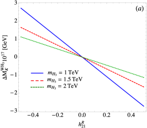
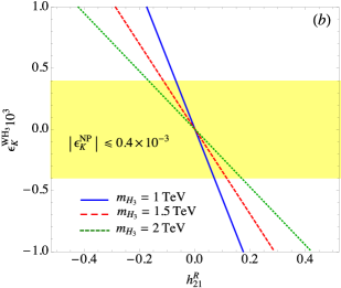
Figure 5: Plots, which are from the $W-{\bf H_{3}}$ box diagrams, for (a) $\Delta M_{K}$ (in units of $10^{-17}$) and (b) $\epsilon_{K}$ (in units of $10^{-3}$) as a function of $h^{R}_{21}$, where the solid, dashed, and dotted lines represent the contributions of $m_{H_{3}}=(1,\,1.5,\,2)$ TeV, respectively. The band denotes the required limit shown in Eq. (104).

V.3 $\Delta M_{K}$ and $\epsilon_{K}$ from ${\cal H}^{H_{3}}_{\Delta S=2}$

As discussed before, eight effective operators are involved in the purely ${\bf H}_{3}$-mediated box diagrams for the $\Delta S=2$ process. Since the hadronic effects have the properties of $P^{VLL(VRR)}_{1}\ll|P^{SLL(SRR)}_{1,2}|$, the contributions from $Q^{VLL(VRR)}_{1}$ are comparable to those from $Q^{SLL(SRR)}_{1,2}$ due to the associated loop functions in the former and latter satisfying $I^{H_{3}}_{B1}(y_{t})\gg I^{H_{3}}_{B2}(y_{t})$. In addition, it can be seen from Eq. (53) that the Wilson coefficients $C^{VLL(RLL)}_{1}$ and $C^{SLL(SRR)}_{1,2}$ depend on $h^{L(R)}_{21}$ in quadratic form. Therefore, it is of interest to understand their contributions to $\Delta M_{K}$ and $\epsilon_{K}$ without the $C^{LR}_{1,2}$ effects, where $C^{LR}_{1,2}\propto h^{L}_{21}h^{R}_{21}$ and the associated loop functions show up in the form of $I^{H_{3}}_{B1}(y_{t})+I^{H_{3}}_{B2}(y_{t})$. Thus, taking $m_{H_{3}}=1.5$ TeV, $h^{L}_{21}=0$, and $h^{R}_{21}=0.11$, where the chosen values obey the bound from $\epsilon^{WH_{3}}_{K}$, we find:

$$\Delta M^{H_{3}}_{K}\approx-2.75\times 10^{-23}~{}\text{GeV}\,,~{}\epsilon^{H_{3}}_{K}\approx-2.90\times 10^{-9}\,.$$ (108)

Clearly, the contributions from the $Q^{VLL(VRR)}_{1}$ and $Q^{SLL(SRR)}_{1,2}$ operators that are induced from the ${\bf H}_{3}$ box diagrams are small and negligible. Since the behavior of $h^{L}_{21}$ is the same as that of $h^{R}_{21}$, the conclusion will not change even with $h^{L}_{21}\sim{\cal O}(10)$, with the exception of $h^{L}_{21}\sim{\cal O}(100)$. In addition, it is not necessary to combine ${\cal H}^{WH_{3}}_{\Delta S=2}$ and ${\cal H}^{H_{3}}_{\Delta S=2}$ because the pure $h^{R}_{21}$ effect in ${\cal H}^{H_{3}}_{\Delta S=2}$ as shown above cannot compete with that in ${\cal H}^{WH_{3}}_{\Delta S=2}$.

The ${\bf H}_{3}$ box diagrams could play an important role through the $C^{LR}_{1,2}$ effects. In addition to the loop function $I^{H_{3}}_{B1}(y_{t})$, the enhancement factors are from the associated hadronic effects $|P^{LR}_{1,2}|$, which are larger than the others. For clarity, we make contour plots for $\Delta M^{H_{3}}_{K}$ (in units of $10^{-17}$) and $\epsilon^{H_{3}}_{K}$ (in unit of $10^{-3}$) as a function of $h^{L}_{21}$ and $h^{R}_{21}$ in Fig. 6, where we fix $m_{H_{3}}=1.5$ TeV. From the plots, we can see that $\Delta M^{H_{3}}_{K}$ is still far below the required limit in the taken ranges of $h^{L,R}_{21}$; however, the allowed parameter spaces of $h^{L,R}_{21}$ could be further limited by the required limit of $|\epsilon^{\rm NP}_{K}|\leq 0.4\times 10^{-3}$.

It can be seen from the Fig. 6(b) that when $|h^{R}_{21}|$ is becoming smaller, the allowed $|h^{L}_{21}|$ is becoming larger due to $C^{LR}_{1,2}\propto h^{L}_{21}h^{R}_{21}$. If we take $h^{R}_{21}\approx 0$, i.e., ${\cal H}^{WH_{3}}_{\Delta S=2}\approx 0$ and $C^{LR}_{1,2}\approx 0$, the $h^{L}_{21}$, dictated by the $Q^{VLL(VRR)}_{1}$ and $Q^{SLL(SRR)}_{1,2}$ effects, can be much larger than ${\cal O}(10)$. Since $h^{L}_{21}$ is defined through $1/|g^{2}V^{*}_{ts}V_{td}|\sim 6.4\times 10^{3}$, $h^{L}_{21}$ of ${\cal O}(30)$ indicates $|g^{L}_{31}|\sim|g^{L}_{32}|\sim 0.07$ and is still in the perturbation range.

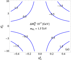
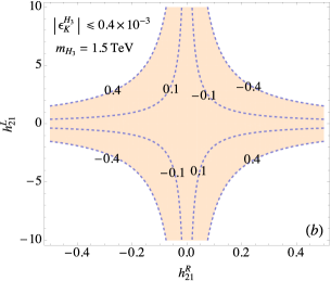
Figure 6: Contours, which arise from the ${\bf H}_{3}-{\bf H}_{3}$ box diagrams, for (a) $\Delta M_{K}$ (in units of $10^{-17}$) and (b) $\epsilon_{K}$ (in units of $10^{-3}$) as a function of $h^{L}_{21}$ and $h^{R}_{21}$, where $m_{H_{3}}=1.5$ TeV is used.

VI Numerical analysis on $\epsilon^{\prime}/\epsilon$ in the diquark model

We numerically study the ${\bf H}_{3}$ contributions to $\epsilon^{\prime}/\epsilon$ in this section. Based on the earlier discussions, it is known that three possible mechanisms can contribute to the Kaon direct CP violation, including the tree-level diagram, the QCD and EW penguins, and the chromomagnetic dipole; in addition, their formulations are given in Eq. (78), Eq. (83), and Eq. (87), respectively. In the following, we discuss their contributions one by one.

VI.1 Tree-level

From $(\epsilon^{\prime}/\epsilon)_{T}^{H_{3}}$ shown in Eq. (78), five free parameters are involved at the tree-level-induced $\Delta S=1$ processes, which are $\zeta^{LL,RR}_{21}$, $\zeta^{RL,LR}_{21}$, and $m_{H_{3}}$. However, it can be seen that the parameter dependence shows up in the form of $\zeta^{RR}_{21}-\zeta^{LL}_{21}$ and $\zeta^{RL}_{21}-\zeta^{LR}_{21}$; thus, it is more convenient to show the numerical analysis if we use these two forms of parameters as the relevant parameters. In addition, since $\zeta^{\chi}_{21}$ is scaled by $V^{*}_{ts}V_{td}$, like the case in $h^{L(R)}_{21}$, where the KM phase is taken as the unique origin of CP violation, we also assume $\zeta^{\chi}_{21}$ to be real parameters in this study although this assumption generally is not necessary.

To illustrate the diquark effects, we show the contours for $Re(\epsilon^{\prime}/\epsilon)^{H_{3}}_{T}$ (in units of $10^{-3}$) as a function of $\zeta^{RR}_{21}-\zeta^{LL}_{21}$ and $\zeta^{RL}_{21}-\zeta^{LR}_{21}$ in Fig. 7(a), where $m_{H_{3}}=1.5$ TeV is used. From the plot, $(\epsilon^{\prime}/\epsilon)^{H_{3}}_{T}$ is insensitive to $\zeta^{RR}_{21}-\zeta^{LL}_{21}$. This behavior can be understood from the small coefficient of $2r_{1}y_{W}/z_{-}$ in $T^{1/2}_{H_{3}}$, where it is above one order of magnitude smaller than $0.67r_{2}y_{W}/(2ReA_{2})$ in $T^{3/2}_{H_{3}}$; that is, $T^{3/2}_{H_{3}}$ dominates the contribution to $(\epsilon^{\prime}/\epsilon)^{H_{3}}_{T}$. Assuming $\zeta^{RR}_{21}=\zeta^{LL}_{21}$, we show the contours for $(\epsilon^{\prime}/\epsilon)^{H_{3}}_{T}$ as a function of $\zeta^{RL}_{21}-\zeta^{LR}_{21}$ and $m_{H_{3}}$ in Fig. 7(b). From these plots, it can be seen that the tree-level diquark effect can significantly enhance $\epsilon^{\prime}/\epsilon$.

To further understand the typical size of the $g^{\chi}_{11(12)}$ parameter, we can take $g^{R}_{11}\sim g^{L}_{12}$ and $|\zeta^{RL}_{21}|\sim 0.5$ as an example. Following $\zeta^{RL}_{21}=g^{R}_{11}g^{L*}_{12}/(g^{2}V^{*}_{ts}V_{td})$, we then obtain $|g^{R}_{11}|\sim|g^{L}_{12}|\sim 0.0088$, which is much smaller than 0.07 the typical value of $g^{\chi}_{31(32)}$ bounded by the $\epsilon^{\rm NP}_{K}$.

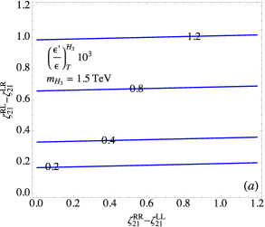
Figure 7: Contours for $\left(\epsilon^{\prime}/\epsilon\right)^{T}_{H_{3}}$ (in units of $10^{-3}$) as a function of (a) $\zeta^{RR}_{21}-\zeta^{LL}_{21}$ and $\zeta^{RL}_{21}-\zeta^{LR}_{21}$ and (b) $m_{H_{3}}$ and $\zeta^{RL}_{21}-\zeta^{LR}_{21}$, where $m_{H_{3}}=1.5$ TeV is used in plot (a), and we assume $\zeta^{RR}_{21}=\zeta^{LL}_{21}$ in plot (b).

VI.2 QCD and EW penguins

According to the formulation of $Re(\epsilon^{\prime}/\epsilon)^{H_{3}}_{P}$ in Eqs. (83) and (84) and the relevant effective Wilson coefficients at $\mu=m_{c}$ defined in Eq. (85), the diquark contributions are dictated by the factors $\delta y^{H_{3}}_{a}$ ($a=3,4,6,7,9$), which exhibit the left-right asymmetry at the $\mu=m_{H_{3}}$ scale. In order to observe the magnitude of each $\delta y^{H_{3}}_{a}$, following Eq. (36) and Eq. (39), we show the $h^{L(R)}_{21}$ dependence with $m_{H_{3}}=1.5$ TeV as:

$$\delta y^{H_{3}}_{3} \approx\left(0.81h^{L}_{21}+0.04h^{R}_{21}\right)\times 10^{-4}\,,$$

$$\delta y^{H_{3}}_{4} \approx 0.11\left(h^{L}_{21}-h^{R}_{21}\right)\times 10^{-4}\,,$$

$$\delta y^{H_{3}}_{5} \approx\left(-0.04h^{L}_{21}+0.89h^{R}_{21}\right)\times 10^{-4}\,,$$

$$\delta y^{H_{3}}_{6} \approx 0.11\left(h^{L}_{21}-h^{R}_{21}\right)\times 10^{-4}\,,$$

$$\delta y^{H_{3}}_{7} \approx\left(0.71h^{L}_{21}-2.54h^{R}_{21}\right)\times 10^{-4}\,,$$

$$\delta y^{H_{3}}_{9} \approx\left(-2.69h^{L}_{21}+0.85h^{R}_{21}\right)\times 10^{-4}\,.$$ (109)

Based on the results, we can understand each $\delta y^{H_{3}}_{a}$ as follows: for $\delta y^{H_{3}}_{3}$, since there is a $y_{W}$ suppression factor in the QCD-penguin, the main contribution is from the $Z$-penguin, i.e. $C^{Z}_{3}\propto I_{Z}h^{L}_{21}$; therefore, it can be seen that the $h^{L}_{21}$ part is much larger than the $h^{R}_{21}$ part. Because $\delta y^{H_{3}}_{4(6)}$ is only from the QCD-penguin, it can be seen that $h^{L}_{21}$ and $h^{R}_{21}$ have equal contributions; in addition, since $y^{(\prime)H_{3}}_{4(6)}$ is a factor of 3 larger than the QCD-penguin part of $y^{(\prime)H_{3}}_{3}$, we therefore see that the $0.11$ factor in $\delta y^{H_{3}}_{4(6)}$ is almost a factor of 3 larger than the $0.04$ appearing in the parentheses of $\delta y^{H_{3}}_{3}$. The behavior of $\delta y^{H_{3}}_{5}$ should be similar to $\delta y^{H_{3}}_{3}$, but it is dominated by $C^{\prime}_{5}\propto I_{Z}h^{R}_{21}$.

Although $\gamma$- and $Z$-penguin both contribute to $\delta y^{H_{3}}_{7}$, due to the $y_{W}$ suppression appearing in $\gamma$-penguin, $\delta y^{H_{3}}_{7}$ indeed is dominated by the $Z$-penguin. It can be found that the $h^{L}_{21}$ and $h^{R}_{21}$ terms in $\delta y^{H_{3}}_{7}$ are different from the $h^{L}_{21}$ term in $\delta y^{H_{3}}_{3}$ and the $h^{R}_{21}$ term in $\delta y^{H_{3}}_{5}$ by factors of $4\sin^{2}\theta_{W}\approx 0.92$ and $-4$, respectively. According to these differences, we can roughly understand the numbers in $\delta y^{H_{3}}_{7}$ from the corresponding numbers in $\delta y^{H_{3}}_{3}$ and $\delta y^{H_{3}}_{5}$. From Eq. (36), $\delta y^{H_{3}}_{9}$ is also dominated by the $Z$-penguin. We find that the $h^{L}_{21}$ and $h^{R}_{21}$ terms in $\delta y^{H_{3}}_{9}$ approximately differ from the corresponding terms in $\delta y^{H_{3}}_{3}$ and $\delta y^{H_{3}}_{5}$ by factors of $-4+4\sin^{2}\theta_{W}\approx-3.08$ and $4\sin^{2}\theta_{W}$, respectively. Using these factors, we then can roughly obtain the numbers in the $\delta y^{H_{3}}_{9}$ from those numbers in $\delta y^{H_{3}}_{3}$ and $\delta y^{H_{3}}_{5}$.

Since $m_{H_{3}}$ is a global parameter in the study, we can simplify the numerical analysis by fixing its value. Hereafter, we fix $m_{H_{3}}=1.5$ GeV in the numerical calculations, unless stated otherwise. Thus, we can implement the results in Eq. (109) to $\Delta y^{H_{3}}_{i}(m_{c})$ (i=4,6,8,9,10) in Eq. (85). Using Eqs. (83) and (84), we plot the contours for $(\epsilon^{\prime}/\epsilon)^{H_{3}}_{P}$ (in units of $10^{-3}$) as a function of $h^{L}_{21}$ and $h^{R}_{21}$ in Fig. 8(a), where the shaded area denotes the constraint of $|\epsilon^{H_{3}}_{K}|\leq 0.4\times 10^{-3}$. From the plot, it can be clearly seen that the diquark parameter spaces, allowed to enhance $\epsilon^{\prime}/\epsilon$, are still wide when the strict bound from $\epsilon_{K}$ is included. In order to understand the role of $a^{1/2}_{H_{3}(0,6)}$ and $a^{3/2}_{H_{3}(0,8)}$, which are defined in Eq. (84), in $\epsilon^{\prime}/\epsilon$, we show each $a^{1/2,3/2}_{H_{3}(0,6,8)}$ effect on $Re(\epsilon^{\prime}/\epsilon)^{H_{3}}_{P}$ in Fig. (8)(b), where the solid, dotted, dashed, and dot-dashed lines denote the contributions of $a^{1/2}_{H_{3}0}$, $a^{1/2}_{H_{3}6}$, $a^{3/2}_{H_{3}0}$, and $a^{3/2}_{H_{3}8}$, respectively, and $h^{R}_{21}=0.11$ is taken. Clearly, $a^{3/2}_{H_{3}8}$ makes the main contribution, and this is because the factor $r_{2}\langle Q_{8}\rangle_{2}/ReA_{2}$ in $a^{3/2}_{H_{3}8}$ is larger than the others by more than one order of magnitude. In addition, it can be seen that in order to obtain positive $(\epsilon^{\prime}/\epsilon)^{H_{3}}_{P}$, $h^{L}_{21}$ prefers negative values. We can simply understand the preference as follows: It is known that $(\epsilon^{\prime}/\epsilon)^{H_{3}}_{P}$ is dominated by $-a^{2/3}_{H_{3}8}\propto-\Delta y^{H_{3}}_{8}(m_{c})\sim-\delta y^{H_{3}}_{7}\propto(-0.71h^{L}_{21}+2.54h^{R}_{21})$. Therefore, a negative $h^{L}_{21}$ can positively enhance $(\epsilon^{\prime}/\epsilon)^{H_{3}}_{P}$.

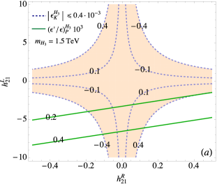
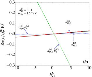
Figure 8: (a) Contours for $(\epsilon^{\prime}/\epsilon)^{H_{3}}_{P}$ (in units of $10^{-3}$) as a function of $h^{L}_{21}$ and $h^{R}_{21}$, where $m_{H_{3}}=1.5$ TeV is used, and the dashed lines and shaded area denote the constraint from $|\epsilon^{H_{3}}_{K}|\leq 0.4\times 10^{-3}$. (b) Each contribution of $a^{1/2}_{H_{3}0}$, $a^{1/2}_{H_{3}6}B^{(1/2)}_{6}$, $a^{3/2}_{H_{3}0}$, and $a^{3/2}_{H_{3}8}B^{3/2}_{8}$ with $m_{H_{3}}=1.5$ TeV and $h^{R}_{21}=0.11$.

VI.3 Chromomagnetic dipole

From Eq. (89), it can be seen that the involved new parameters contributing to $\epsilon^{\prime}/\epsilon$ through the CMOs are $h^{L,R}_{12}$ and simply appear in the form of $h^{R}_{21}-h^{L}_{21}$. With $m_{H_{3}}=1.5$ TeV, we show the contours for $(\epsilon^{\prime}/\epsilon)^{H_{3}}_{8G}$ (in units of $10^{-3}$) as a function of $h^{L}_{21}$ and $h^{R}_{21}$ in Fig. 9, where the shaded area denotes the constraint of $\epsilon^{H_{3}}_{K}\leq 0.4\times 10^{-3}$. From the results, we can see that the $\epsilon^{\prime}/\epsilon$ can be significantly enhanced by the CMOs in the diquark model when the bound from the $\epsilon_{K}$ is satisfied. Due to the dependence of $h^{R}_{21}-h^{L}_{21}$, a negative $h^{L}_{21}$ can lead to a positive $(\epsilon^{\prime}/\epsilon)^{H_{3}}_{8G}$. Comparing the results with those in $(\epsilon^{\prime}/\epsilon)^{H_{3}}_{P}$, it can be found that $(\epsilon^{\prime}/\epsilon)^{H_{3}}_{8G}$ is larger than $(\epsilon^{\prime}/\epsilon)^{H_{3}}_{P}$ in the same allowed parameter space of $h^{L}_{21}$.

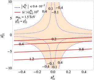
Figure 9: The legend is the same as that in Fig. 8(a) with the exception of $(\epsilon^{\prime}/\epsilon)^{H_{3}}_{8G}$.

VII Summary

We investigated the color-triplet diquark ${\bf H}_{3}$ contributions to the $\Delta S=2$ and $\Delta S=1$ processes in detail. In addition to the ${\bf H}_{3}$ Yukawa couplings to the SM quarks, we also derive the strong and electroweak gauge couplings to ${\bf H}_{3}$. Using the obtained couplings, we calculated renormalized vertex functions for $d\to s(g^{(*)},\gamma^{(*)},Z)$. Based on the results, we studied the implications on the Kaon direct and indirect CP violation.

We found that the box diagrams mediated by one $W(G)$-boson and one ${\bf H}_{3}$ for $\Delta S=2$, which were neglected in Barr:1989fi , play an important role on the constraint of the parameter $h^{R}_{21}$ when the sizable top-quark mass is taken. The constraint on $h^{L}_{21}$ can be achieved through the purely ${\bf H}_{3}$-mediated box diagrams.

It was found that three potential mechanisms could enhance the Kaon direct CP violation parameter $\epsilon^{\prime}/\epsilon$, such as the tree-level diagram, the QCD and electroweak penguins, and the chromomagnetic dipole operators. To clearly see each effect, we separately discuss their contributions. In order to study the $\epsilon^{\prime}/\epsilon$, in this work, we simply assume that the CP violating origin only arises from the so-called KM phase of the CKM matrix in the SM. Using the limited parameters and the hadronic matrix elements provided in Aebischer:2018rrz , we find that the $\Delta S=2$ process cannot give a strict bound on the tree-level parameters $\zeta^{RR,LL}_{21}$ and $\zeta^{RL,LR}_{21}$; therefore, the parameter spaces to significantly enhance $(\epsilon^{\prime}/\epsilon)$ are wide.

The parameters associated with the QCD and electroweak penguins and the chromomagnetic dipole are the same. Although these parameters used to enhance $\epsilon^{\prime}/\epsilon$ are bounded by the Kaon indirect CP violation $\epsilon_{K}$, it was found that $\epsilon^{\prime}/\epsilon$ can still be significantly enhanced by these mechanisms. In addition, in the same parameter space of $h^{L}_{21}$, which can generate a sizable $\epsilon^{\prime}/\epsilon$, the contribution to $\epsilon^{\prime}/\epsilon$ from the chromomagnetic operators is larger than that from the QCD and EW penguins.

Appendix A

A.1 Renormalized two- and three-point diagrams for gluon emission

To deal with the calculations of one-loop Feynman diagrams, we show the useful $d$-dimensional integral as:

$$J(d,m,n,\mu^{2}_{B}) =\int\frac{d^{d}\ell}{(2\pi)^{d}}\frac{(\ell^{2})^{m}}{(\ell^{2}-\mu^{2}_{B})^{n}}$$

$$=i\frac{(-1)^{m-n}(\mu^{2}_{B})^{d/2+m-n}}{(4\pi)^{d/2}}\frac{\Gamma(n-m-d/2)\Gamma(m+d/2)}{\Gamma(d/2)\Gamma(n)}\,.$$ (110)

Using dimensional regulation with $d=4+2\epsilon$, renormalization scale $\mu$, and $\Gamma(-\epsilon)=-1/\epsilon-\gamma_{E}$, the relevant integrals in the study are explicitly written as:

$$J(d,0,2,\mu^{2}_{B}) =i\frac{\mu^{2\epsilon}}{(4\pi)^{2}}\ln\frac{\Lambda^{2}}{\mu^{2}_{B}}\,,$$

$$J(d,0,3,\mu^{2}_{B}) =-i\frac{1}{(4\pi)^{2}\Gamma(3)}\frac{1}{\mu^{2}_{B}}\,,$$

$$J(d,1,3,\mu^{2}_{B}) =\frac{d}{4}J(d,0,2,\mu^{2}_{B})\,,$$ (111)

where we define $\ln\Lambda^{2}=-1/\epsilon-\gamma_{E}+\ln(4\pi\mu^{2})$, and $\gamma_{E}$ is the Euler-Mascheroni constant.

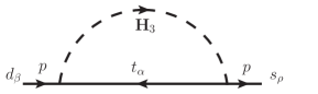
Figure 10: Self-energy diagram for the $d\to s$ transition mediated by color-triplet diquark ${\bf H}_{3}$.

The self-energy diagram mediated by ${\bf H}_{3}$ for the $d\to s$ transition is sketched in Fig. 10. Using the Yukawa couplings in Eq. (11), the result of Fig. 10 can be expressed as:

$$i\Sigma(p) =\bar{s}\,\Gamma\,d=\bar{s}\left[\not{p}\chi^{V}_{21}\int^{1}_{0}dx\,xJ(d,0,2,\mu^{2}_{B1}(p^{2}))\right.$$

$$\left.+m_{t}\chi^{S}_{21}\int^{1}_{0}dx\,J(d,0,2,\mu^{2}_{B1}(p^{2}))\right]d\,,$$ (112)

$$\chi^{V}_{21} =g^{L*}_{32}g^{L}_{31}P_{L}+g^{R*}_{32}g^{R}_{31}P_{R}\,,$$

$$\chi^{S}_{21} =g^{R*}_{32}g^{L}_{31}P_{L}+g^{L*}_{32}g^{R}_{31}P_{R}\,,$$ (113)

where $(K^{a})^{\rho\alpha}(\bar{K}_{a})_{\alpha\beta}=\delta_{\beta}^{\rho}$ is used, and $\mu^{2}_{B1}(p^{2})=m^{2}_{H_{3}}x+m_{t}^{2}(1-x)-p^{2}x(1-x)$. To obtain the renormalized $\Gamma$, we require $\Sigma(p)=0$ when the momentum of the external quark is taken on the mass shell, i.e., $p=p_{d}$ or $p=p_{s}$. If we write the renormalized $\Gamma_{R}$ as:

$$\Gamma_{R}=\Gamma+C_{1}\not{p}P_{L}+C_{2}\not{p}P_{R}+C_{3}P_{R}+C_{4}P_{L}\,,$$ (114)

the requirements of $\Sigma_{R}(p_{d})=0$ and $\Sigma_{R}(p_{s})=0$ lead to

$$C_{1}\simeq-g^{L*}_{32}g^{L}_{31}\int^{1}_{0}dx\,xJ(d,0,2,\mu^{2}_{B1}(0))\,,$$

$$C_{2}\simeq-g^{R*}_{32}g^{R}_{31}\int^{1}_{0}dx\,xJ(d,0,2,\mu^{2}_{B1}(0))\,,$$

$$C_{3}\simeq-g^{L*}_{32}g^{R}_{31}m_{t}\int^{1}_{0}dx\,J(d,0,2,\mu^{2}_{B1}(0))\,,$$

$$C_{4}\simeq-g^{R*}_{32}g^{L}_{31}m_{t}\int^{1}_{0}dx\,J(d,0,2,\mu^{2}_{B1}(0))\,,$$ (115)

where we have dropped the light quark mass effects. We note that the mass dimension in $C_{1(2)}$ is different from that in $C_{3(4)}$.

The color-triplet-mediated three-point diagrams for $d\to sg^{(*)}$ are shown in Fig. 2, where $g^{(*)}$ denotes the on-shell (off-shell) gluon. The result of Fig. 2(a), where the gluon is emitted from the top-quark, is given as:

$$i\Gamma^{A\mu}_{a} =g_{s}(K^{b})^{\rho\sigma}(T^{A})^{\alpha}_{\sigma}(\bar{K}_{b})_{\alpha\beta}\Gamma(3)\int^{1}_{0}dx_{1}\int^{x_{1}}_{0}dx_{2}\int\frac{d^{d}\ell}{(2\pi)^{d}}\frac{1}{(\ell^{2}-\mu^{2}_{B2}(k^{2}))^{3}}$$

$$\times\bar{s}_{\rho}\left\{-A^{\mu}_{1}\chi^{V}_{21}+A^{\mu}_{2}\chi^{S}_{21}\right\}d^{\beta}\,,$$ (116)

$$A^{\mu}_{1} =\not{\ell}\gamma^{\mu}\not{\ell}+[m^{2}_{t}-k^{2}x_{2}(x_{2}-x_{1})]\gamma^{\mu}\,,$$

$$A^{\mu}_{2} =m_{t}[(x_{2}-x_{1})\gamma^{\mu}\not{k}+x_{2}\not{k}\gamma^{\mu}]\,,$$

$$\mu^{2}_{B2}(k^{2}) =m^{2}_{H_{3}}(1-x_{1})+m^{2}_{t}x_{1}+k^{2}x_{2}(x_{2}-x_{1})\,,$$ (117)

where $T^{A}$ are the generators of $SU(3)_{C}$ and their normalizations are taken as $Tr(T^{A}T^{B})=\delta^{AB}/2$. We find that the color factor and the ultraviolet divergent part can be expressed as:

$$(K^{b})^{\rho\sigma}(T^{A})^{\alpha}_{\sigma}(\bar{K}_{b})_{\alpha\beta} =-\frac{(T^{A})^{\rho}_{\beta}}{2}\,,$$

$$\int\frac{d^{d}\ell}{(2\pi)^{d}}\frac{\not{\ell}\gamma^{\mu}\not{\ell}}{(\ell^{2}-\mu^{2}_{B_{2}}(k^{2}))^{3}} =-\gamma^{\mu}\frac{1+\epsilon}{\Gamma(3)}J(d,0,2,\mu^{2}_{B_{2}}(k^{2}))\,.$$ (118)

Accordingly, $\Gamma^{A\mu}_{a}$ can be reformulated as:

$$i\Gamma^{A\mu}_{a} =-i\frac{g_{s}}{2(4\pi)^{2}}\bar{s}\gamma^{\mu}\chi^{V}_{21}T^{A}d\int^{1}_{0}dx_{1}\int^{x_{1}}_{0}dx_{2}$$

$$\times\left[\mu^{2\epsilon}\left(\ln\frac{\Lambda^{2}}{\mu^{2}_{B2}(k^{2})}-1\right)+\frac{m^{2}_{t}+k^{2}x_{2}(x_{2}-x_{1})}{\mu^{2}_{B2}(k^{2})}\right]$$

$$+i\frac{g_{s}}{2(4\pi)^{2}}\bar{s}A^{\mu}_{2}\chi^{S}_{21}T^{A}d\int^{1}_{0}dx_{1}\int^{x_{1}}_{0}dx_{2}\frac{1}{\mu^{2}_{B2}(k^{2})}\,.$$ (119)

Using the diquark-gluon coupling shown in Eq. (17), the result of Fig. 2(b), where the gluon is emitted from the ${\bf H_{3}}$, can be obtained as:

$$i\Gamma^{A\mu}_{b} =g_{s}(K^{a})^{\rho\alpha}(\bar{K}_{b})_{\alpha\beta}(t^{A})^{b}_{a}\Gamma(3)\int^{1}_{0}dx_{1}\int^{x_{1}}_{0}dx_{2}\int\frac{d^{d}\ell}{(2\pi)^{d}}\frac{1}{(\ell^{2}-\mu^{2}_{B3}(k^{2}))^{3}}$$

$$\times\bar{s}_{\rho}\left\{-B^{\mu}_{1}\chi^{V}_{21}+B^{\mu}_{2}\chi^{S}_{21}\right\}d^{\beta}\,,$$ (120)

$$B^{\mu}_{1} =2\ell^{\mu}\not{\ell}\,,~{}~{}B^{\mu}_{2}=m_{t}[p^{\mu}_{s}(2-2x_{1})-k^{\mu}(1-2x_{1}+2x_{2})]\,,$$

$$\mu^{2}_{B3}(k^{2}) =m^{2}_{H_{3}}x_{1}+m^{2}_{t}(1-x_{1})+k^{2}x_{2}(x_{2}-x_{1})\,,$$ (121)

where $(t^{A})^{b}_{a}=2Tr(\bar{K}_{a}T^{A}K^{b})$ denotes the effective color factor. Similar to Eq. (116), the color factor and ultraviolet divergent part of Fig. 2(b) can be obtained as:

$$(K^{a})^{\rho\alpha}(\bar{K}_{b})_{\alpha\beta}(t^{A})^{b}_{a} =2(K^{a})^{\rho\alpha}(\bar{K}_{b})_{\alpha\beta}Tr\bar{K}_{a}T^{A}K^{b}=\frac{(T^{A})_{\beta}^{\rho}}{2}\,,$$

$$\int\frac{d^{d}\ell}{(2\pi)^{d}}\frac{\ell^{\mu}\not{\ell}}{(\ell^{2}-\mu^{2}_{B_{3}}(k^{2}))^{3}} =\frac{\gamma^{\mu}}{2\Gamma(3)}J(d,0,2,\mu^{2}_{B3})\,.$$ (122)

Thus, the vertex function for the gluon emitting from the diquark is given by:

$$i\Gamma^{A\mu}_{b} =-i\frac{g_{s}}{2(4\pi)^{2}}\bar{s}\gamma^{\mu}\chi^{V}_{21}T^{A}d\int^{1}_{0}dx_{1}\int^{x_{1}}_{0}dx_{2}\mu^{2\epsilon}\ln\frac{\Lambda^{2}}{\mu^{2}_{B3}(k^{2})}$$

$$-i\frac{g_{s}}{2(4\pi)^{2}}\bar{s}\chi^{S}_{21}T^{A}d\int^{1}_{0}dx_{1}\int^{x_{1}}_{0}dx_{2}\frac{B^{\mu}_{2}}{\mu^{2}_{B3}(k^{2})}\,.$$ (123)

From the Ward-Takahashi identity, it is known that the three-point vertex correction can be related to the two-point function $\Sigma(p)=\bar{s}\Gamma d$ through the relation:

$$k_{\mu}\Gamma^{A\mu}=k_{\mu}\Gamma^{A\mu}_{a+b}=g_{s}(T^{A})_{\beta}^{\rho}\left[\Sigma(p-k)_{\rho}^{\beta}-\Sigma(p)_{\rho}^{\beta}\right],$$ (124)

with $\Sigma(p)_{\rho}^{\beta}=\bar{s}_{\rho}\Gamma d^{\beta}$. In order to obtain the renormalized $\Gamma^{A\mu}$, we can require that the Ward-Takahashi identity is retained as $k_{\mu}\Gamma^{A\mu}_{R}=g_{s}(T^{A})^{\rho}_{\beta}\left[\Sigma_{R}(p-k)_{\rho}^{\beta}-\Sigma_{R}(p)_{\rho}^{\beta}\right]$ Chia:1983hd ; Davies:1991jt . If we set $\Gamma^{A\mu}_{R}=\Gamma^{A\mu}+X^{A\mu}$, the Ward-Takahashi identity can lead to:

$$X^{A\mu} =\bar{s}\gamma^{\mu}\chi^{V}_{21}T^{A}d\int^{1}_{0}dx\,xJ(d,0,2,\mu^{2}_{B1}(0))$$

$$=\frac{i}{(4\pi)^{2}}\bar{s}\gamma^{\mu}\chi^{V}_{21}T^{A}d\int^{1}_{0}dx\,x\mu^{2\epsilon}\ln\frac{\Lambda^{2}}{\mu^{2}_{B1}(0)}\,.$$ (125)

The ultraviolet divergence of $\Gamma^{A\mu}_{R}$, which is related to $\ln\Lambda^{2}$ terms, can then be cancelled as:

$$\Gamma^{A\mu}_{R}\Big{|}_{\rm div}=\Gamma^{A\mu}_{a+b}\Big{|}_{\rm div}+X^{A\mu}\Big{|}_{\rm div}\propto-\int^{1}_{0}dx_{1}\int^{x_{1}}_{0}dx_{2}\frac{\ln\Lambda^{2}}{2}\times 2+\int^{1}_{0}dx\,x\ln\Lambda^{2}=0\,.$$ (126)

In order to verify the gauge invariance, we can take $k^{2}=0$ for the on-shell gluon; thus, the Ward identity can be satisfied as:

$$k_{\mu}\Gamma^{A\mu}_{R} \propto\int^{1}_{0}dx_{1}\int^{x_{1}}_{0}dx_{2}\frac{1}{2}\left[\left(\ln\frac{\mu^{2}_{B2}(0)}{m^{2}_{H_{3}}}+1\right)-\frac{m^{2}_{t}}{\mu^{2}_{B2}(0)}+\ln\frac{\mu^{2}_{B3}(0)}{m^{2}_{H_{3}}}\right]$$

$$+\int^{1}_{0}dx\,x\,\ln\frac{\mu^{2}_{B1}(0)}{m^{2}_{H_{3}}}$$

$$=\frac{1}{4}+\frac{1}{2}\int^{1}_{0}dx\left[(1-2x)\ln(x+y_{t}(1-x))-\frac{y_{t}(1-x)}{x+y_{t}(1-x)}\right]=0\,,$$ (127)

with $y_{t}=m^{2}_{t}/m^{2}_{H_{3}}$. For $k^{2}\neq 0$, due to $k^{2}\ll m^{2}_{t}$, the leading $k^{2}$ term and chromomagnetic dipole effect of $\Gamma^{A\mu}_{R}$ can be obtained as:

$$i\epsilon^{A}_{\mu}\Gamma^{A\mu}_{R} =-i\frac{g_{s}k^{2}}{(4\pi)^{2}m^{2}_{H_{3}}}I_{G1}(y_{t})\bar{s}\not{\epsilon}^{A}\chi^{V}_{21}T^{A}d+i\frac{g_{s}}{(4\pi)^{2}}\frac{m_{t}}{4m^{2}_{H_{3}}}I_{G2}(y_{t})\bar{s}\sigma^{\mu\nu}\chi^{S}_{21}T^{A}d\,G^{A}_{\mu\nu}\,,$$ (128)

where the loop-integral functions are given as:

$$I_{G1}(y) =\frac{2y^{2}+11y-7}{36(1-y)^{3}}+\frac{(y^{3}+3y-2)\ln y}{12(1-y)^{4}}\,,$$

$$I_{G2}(y) =-\frac{1}{(1-y)}-\frac{\ln y}{(1-y)^{2}}\,.$$ (129)

A.2 Renormalized three-point vertex function for $d\to s\gamma^{(*)}$

In addition to the gluon-penguin diagrams, the electroweak penguin diagrams, i.e. $d\to s\gamma^{*}(Z^{*})$, also make significant contributions to $\epsilon^{\prime}/\epsilon$. Since photon is a massless particle, like the case in the $d\to sg^{*}$ process, the leading effect for the photon emission $d\to s\gamma^{*}$ decay should be proportional to $k^{2}$, so that the off-shell photon propagator of $1/k^{2}$ in the $d\to sq\bar{q}$ processes can be cancelled. Due to the similarity to the gluon case, in this subsection, we first discuss the $d\to s\gamma^{(*)}$ process.

The Feynman diagrams for $d\to s\gamma^{(*)}$ are shown in Fig. 3. It can be seen that with the exception of gauge couplings, the calculations for $d\to s\gamma^{(*)}$ are similar to those for $d\to sg^{(*)}$; therefore, the results of Fig. 3(a) and (b) can be respectively obtained from Eqs. (119) and (123), when the strong interactions are replaced by the electromagnetic interactions. Thus, using $(K^{a})^{\alpha\beta}(\bar{K}_{a})_{\rho\alpha}=\delta^{\beta}_{\rho}$ and gauge coupling in Eq. (22), the results of Fig. 3(a) and (b) can be formulated as:

$$i\Gamma^{\mu}_{\gamma a} =i\frac{e_{t}e}{(4\pi)^{2}}\bar{s}\gamma^{\mu}\chi^{V}_{21}d\int^{1}_{0}dx_{1}\int^{x_{1}}_{0}dx_{2}$$

$$\times\left[\mu^{2\epsilon}\left(\ln\frac{\Lambda^{2}}{\mu^{2}_{B2}(k^{2})}-1\right)+\frac{m^{2}_{t}+k^{2}x_{2}(x_{2}-x_{1})}{\mu^{2}_{B2}(k^{2})}\right]$$

$$-i\frac{e_{t}e}{(4\pi)^{2}}\bar{s}A^{\mu}_{2}\chi^{S}_{21}d\int^{1}_{0}dx_{1}\int^{x_{1}}_{0}dx_{2}\frac{1}{\mu^{2}_{B2}(k^{2})}\,.$$ (130)

$$i\Gamma^{\mu}_{\gamma b} =-i\frac{e_{t}e}{(4\pi)^{2}}\bar{s}\gamma^{\mu}\chi^{V}_{21}d\int^{1}_{0}dx_{1}\int^{x_{1}}_{0}dx_{2}\mu^{2\epsilon}\ln\frac{\Lambda^{2}}{\mu^{2}_{B3}(k^{2})}$$

$$-i\frac{e_{H_{3}}e}{(4\pi)^{2}}\bar{s}\chi^{S}_{21}d\int^{1}_{0}dx_{1}\int^{x_{1}}_{0}dx_{2}\frac{B^{\mu}_{2}}{\mu^{2}_{B3}(k^{2})}\,,$$ (131)

where $\chi^{V(S)}_{21}$, $A^{\mu}_{2}$, and $B^{\mu}_{2}$ can be found in Eqs. (113), (117), and (121), respectively. In order to obtain the renormalized vertex function, we require that the Ward-Takahashi identity, which is defined as:

$$k_{\mu}\Gamma^{\mu}_{\gamma}=k_{\mu}(\Gamma^{\mu}_{\gamma a}+\Gamma^{\mu}_{\gamma b})=e_{d}e[\Sigma(p-k)-\Sigma(p)]\,,$$ (132)

is retained when we renormalize the three-point vertex corrections, i.e., $k_{\mu}\Gamma^{\mu}_{\gamma R}=e_{d}e[\Sigma_{R}(p-k)-\Sigma_{R}(p)]$, where $e_{d}$ denotes the electric charge of a down-type quark, and $\Sigma_{R}(p)$ can be obtained from Eq. (114). If we set $\Gamma^{\mu}_{\gamma R}=\Gamma^{\mu}_{\gamma}+X^{\mu}_{\gamma}$, the renormalization requirement can lead to:

$$X^{\mu}_{\gamma}=i\frac{e_{d}e}{(4\pi)^{2}}\bar{s}\gamma^{\mu}\chi^{V}_{21}d\int^{1}_{0}dx\,x\,\mu^{2\epsilon}\ln\frac{\Lambda^{2}}{\mu^{2}_{B1}(0)}\,.$$ (133)

Similar to the gluon penguin, the $\ln\Lambda^{2}$ ultraviolet divergence related terms in $\Gamma^{\mu}_{R}$ can be cancelled as:

$$\Gamma^{\mu}_{\gamma R}\Big{|}_{\rm div} =\Gamma^{\mu}_{\gamma(a+b)}\Big{|}_{\rm div}+X^{\mu}_{\gamma}\Big{|}_{\rm div}$$

$$\propto(e_{t}-e_{H_{3}})\int^{1}_{0}dx_{1}\int^{x_{1}}_{0}dx_{2}\ln\Lambda^{2}+e_{d}\int^{1}_{0}dx\,x\ln\Lambda^{2}=0\,.$$ (134)

We can verify the $U(1)_{\rm em}$ gauge invariance through the case of $k^{2}=0$ as:

$$k_{\mu}\Gamma^{\mu}_{\gamma R} \propto e_{t}\int^{1}_{0}dx_{1}\int^{x_{1}}_{0}dx_{2}\left[\left(-\ln\frac{\mu^{2}_{B2}(0)}{m^{2}_{H_{3}}}-1\right)+\frac{m^{2}_{t}}{\mu^{2}_{B2}(0)}\right]$$

$$+e_{H_{3}}\int^{1}_{0}dx_{1}\int^{x_{1}}_{0}dx_{2}\ln\frac{\mu^{2}_{B3}(0)}{m^{2}_{H_{3}}}-e_{d}\int^{1}_{0}dx\,x\,\ln\frac{\mu^{2}_{B1}(0)}{m^{2}_{H_{3}}}$$

$$=-\frac{1}{3}-\frac{2}{3}\int^{1}_{0}dx\left[(1-2x)\ln(x+y_{t}(1-x))-\frac{y_{t}(1-x)}{x+y_{t}(1-x)}\right]=0\,.$$ (135)

Hence, the leading $k^{2}$ and electromagnetic dipole effects of $\Gamma^{\mu}_{R}$ can be obtained as:

$$i\epsilon_{\mu}\Gamma^{\mu}_{\gamma R} =-i\frac{ek^{2}}{3(4\pi)^{2}m^{2}_{H_{3}}}I_{\gamma 1}(y_{t})\bar{s}\not{\epsilon}\chi^{V}_{21}d-i\frac{e}{(4\pi)^{2}}\frac{m_{t}}{6m^{2}_{H_{3}}}I_{\gamma 2}(y_{t})\bar{s}\sigma^{\mu\nu}\chi^{S}_{21}d\,F_{\mu\nu}\,,$$ (136)

where the loop-integral functions are given as:

$$I_{\gamma 1}(y) =\frac{25y^{2}-65y+34}{36(1-y)^{3}}+\frac{y^{3}+2(2-3y)}{6(1-y)^{4}}\ln y\,,$$

$$I_{\gamma 2}(y) =-\frac{7-y}{2(1-y)^{2}}-\frac{(2+y)\ln y}{(1-y)^{3}}\,.$$ (137)

A.3 Renormalized three-point vertex function for $d\to sZ^{*}$

To calculate the $Z$-penguin induced three-point vertex for $d\to sZ^{*}$, we write the $Z$-couplings to quarks as:

$${\cal L}_{Zqq} =-\frac{g}{\cos\theta_{W}}\bar{q}\gamma_{\mu}(C^{q}_{L}P_{L}+C^{q}_{R}P_{R})Z^{\mu}\,,$$ (138)

$$C^{q}_{L} =I^{q}-e_{q}\sin^{2}\theta_{W}\,,~{}C^{q}_{R}=-e_{q}\sin^{2}\theta_{W}\,,$$ (139)

where $I^{q}$ and $e_{q}$ are the weak isospin and electric charge of the $q$-quark, respectively. From the $Z$-boson interactions, it can be seen that the $e_{t}\sin^{2}\theta_{W}$ related currents indeed are the same as the electromagnetic currents; that is, the corresponding three-point vertex function should be proportional to $k^{2}$. Since $Z$-boson is a massive particle, unlike the case in $d\to s\gamma^{*}$, the $k^{2}$-related effects will be suppressed by $k^{2}/m^{2}_{Z}$ in the decays such as $d\to sq\bar{q}$ and $d\to s\ell\bar{\ell}$. Thus, we expect that the renormalized $d\to sZ^{*}$ vertex is only related to the weak isospin $I^{t}=1/2$ when the $k^{2}$ effects are neglected. In the following, we show the calculated results.

Using the Yukawa couplings shown in Eq. (11), the relation $(K^{a})^{\rho\alpha}(\bar{K}_{a})_{\alpha\beta}=\delta^{\rho}_{\beta}$, and the integrals in Eq. (111), the results of Fig. 3(a) and (b) can be respectively expressed as:

$$i\Gamma^{\mu}_{Za} =i\frac{g}{(4\pi)^{2}\cos\theta_{W}}\int^{1}_{0}dx_{1}\int^{x_{1}}_{0}dx_{2}$$

$$\times\left[\mu^{2\epsilon}\left(\ln\frac{\Lambda^{2}}{\mu^{2}_{B2}(0)}-1\right)\bar{s}\gamma^{\mu}\xi^{t}_{21}d+\frac{m^{2}_{t}}{\mu^{2}_{B2}(0)}\bar{s}\gamma^{\mu}\eta^{t}_{21}d\right]\,,$$ (140)

$$i\Gamma^{\mu}_{Zb} =i\frac{ge_{H_{3}}\sin^{2}\theta_{W}}{(4\pi)^{2}\cos\theta_{W}}\bar{s}\gamma^{\mu}\chi^{V}_{21}d\int^{1}_{0}dx_{1}\int^{x_{1}}_{0}dx_{2}\mu^{2\epsilon}\ln\frac{\Lambda^{2}}{\mu^{2}_{B3}(0)}\,,$$ (141)

$$\xi^{q}_{21} =g^{L}_{31}g^{L*}_{21}C^{q}_{L}P_{L}+g^{R}_{31}g^{R*}_{32}C^{q}_{R}P_{R}\,,$$

$$\eta^{q}_{21} =g^{L}_{31}g^{L*}_{21}C^{q}_{R}P_{L}+g^{R}_{31}g^{R*}_{32}C^{q}_{L}P_{R}\,,$$

where we have taken $k^{2}=0$ and dropped the small effect from the dipole operators.

The Ward-Takahashi identity for the $d\to sZ^{*}$ vertex is given by:

$$k_{\mu}\Gamma^{\mu}_{Z}=k_{\mu}(\Gamma^{\mu}_{Za}+\Gamma^{\mu}_{Zb})=\frac{g}{\cos\theta_{W}}\left(\Sigma^{\prime}(p-k)-\Sigma^{\prime}(p)\right)\,,$$ (142)

where $\Sigma^{\prime}(p)$ can be obtained from the $\Sigma(p)$ in Eq. (112) using $\xi^{d}_{21}$ instead of $\chi^{V}_{21}$. If the renormalized $\Gamma^{\mu}_{Z}$ is written as $\Gamma^{\mu}_{ZR}=\Gamma^{\mu}_{Z}+X^{\mu}_{Z}$, by requiring $\Gamma^{\mu}_{ZR}$ to obey the same Ward-Takahashi identity as shown in Eq. (142), $X^{\mu}_{Z}$ can be found as:

$$X^{\mu}_{Z}=i\frac{g}{(4\pi)^{2}\cos\theta_{W}}\bar{s}\gamma^{\mu}\xi^{d}_{21}d\int^{1}_{0}dx\,x\,\mu^{2\epsilon}\ln\frac{\Lambda^{2}}{\mu^{2}_{B1}(0)}$$ (143)

Thus, we can check the UV divergence-free as follows:

$$\Gamma^{\mu}_{ZR}\Big{|}_{\rm div}=\Gamma^{\mu}_{Z(a+b)}\Big{|}_{\rm div}+X^{\mu}_{Z}\Big{|}_{\rm div} \propto\bar{s}\gamma^{\mu}P_{L}d\,\ln\Lambda^{2}g^{L}_{31}g^{L*}_{32}\left(C^{t}_{L}+e_{H_{3}}\sin^{2}\theta_{W}+C^{d}_{L}\right)$$

$$+\bar{s}\gamma^{\mu}P_{R}d\,\ln\Lambda^{2}g^{R}_{31}g^{R*}_{32}\left(C^{t}_{R}+e_{H_{3}}\sin^{2}\theta_{W}+C^{d}_{R}\right)=0\,,$$ (144)

where the vanished result arises from $-e_{t}+e_{H_{3}}-e_{d}=0$.

It was mentioned earlier that the contribution of electromagnetism-like $Z$ coupling to top-quark vanishes at $k^{2}=0$. In order to verify this result, we can focus on the effects of $e_{f}\sin^{2}\theta_{W}$ that appear in the $Z$-coupling. Thus, using $e_{t}=e_{H_{3}}-e_{d}$, the renormalized vertex function can be expressed as:

$$i\Gamma^{\mu}_{ZR} \supset-i\frac{ge_{t}\sin^{2}\theta_{W}}{(4\pi)^{2}\cos\theta_{W}}\bar{s}\gamma^{\mu}\chi^{V}_{21}d$$

$$\times\left[\frac{1}{2}+\int^{1}_{0}dx(1-2x)\ln(x+y_{t}(1-x))-\frac{y_{t}(1-x)}{x+y_{t}(1-x)}\right]=0$$ (145)

It can be found that the vanished result indeed is similar to that shown in Eqs. (127) and (135). Hence, the renormalized three-point vertex can be obtained as:

$$i\epsilon^{Z}_{\mu}\Gamma^{\mu}_{ZR}=-i\frac{gI^{t}}{(4\pi)^{2}\cos\theta_{W}}\bar{s}\not{\epsilon}^{Z}\left(g^{L}_{31}g^{L*}_{32}I_{Z}(y_{t})P_{L}-g^{R}_{31}g^{R*}_{32}I_{Z}(y_{t})P_{R}\right)d\,,$$ (146)

where the resulted vertex function is associated with the top-quark weak isospin $I^{t}=1/2$, and the loop integral $I_{Z}(y_{t})$ is defined as:

$$I_{Z}(y) =-\frac{y}{1-y}-\frac{y\ln y}{(1-y)^{2}}\,.$$ (147)

References

- (1) N. Cabibbo, Phys. Rev. Lett. 10, 531 (1963).
- (2) M. Kobayashi and T. Maskawa, Prog. Theor. Phys. 49, 652 (1973).
- (3) P. A. Boyle et al. [RBC and UKQCD Collaborations], Phys. Rev. Lett. 110, no. 15, 152001 (2013) [arXiv:1212.1474 [hep-lat]].
- (4) T. Blum et al., Phys. Rev. Lett. 108, 141601 (2012) [arXiv:1111.1699 [hep-lat]].
- (5) T. Blum et al., Phys. Rev. D 86, 074513 (2012) [arXiv:1206.5142 [hep-lat]].
- (6) T. Blum et al., Phys. Rev. D 91, no. 7, 074502 (2015) [arXiv:1502.00263 [hep-lat]].
- (7) Z. Bai et al. [RBC and UKQCD Collaborations], Phys. Rev. Lett. 115, no. 21, 212001 (2015) [arXiv:1505.07863 [hep-lat]].
- (8) J. R. Batley et al. [NA48 Collaboration], Phys. Lett. B 544, 97 (2002) [hep-ex/0208009].
- (9) A. Alavi-Harati et al. [KTeV Collaboration], Phys. Rev. D 67, 012005 (2003) Erratum: [Phys. Rev. D 70, 079904 (2004)] [hep-ex/0208007].
- (10) E. Abouzaid et al. [KTeV Collaboration], Phys. Rev. D 83, 092001 (2011) [arXiv:1011.0127 [hep-ex]].
- (11) A. J. Buras and J. M. Gerard, JHEP 1512, 008 (2015) [arXiv:1507.06326 [hep-ph]].
- (12) A. J. Buras, M. Gorbahn, S. Jager and M. Jamin, JHEP 1511, 202 (2015) [arXiv:1507.06345 [hep-ph]].
- (13) T. Kitahara, U. Nierste and P. Tremper, JHEP 1612, 078 (2016) [arXiv:1607.06727 [hep-ph]].
- (14) A. J. Buras and J. M. Gèrard, Nucl. Phys. B 264, 371 (1986).
- (15) W. A. Bardeen, A. J. Buras and J. M. Gerard, Phys. Lett. B 180, 133 (1986).
- (16) W. A. Bardeen, A. J. Buras and J. M. Gèrard, Nucl. Phys. B 293, 787 (1987).
- (17) W. A. Bardeen, A. J. Buras and J. M. Gèrard, Phys. Lett. B 192, 138 (1987).
- (18) W. A. Bardeen, A. J. Buras and J. M. Gèrard, Phys. Lett. B 211, 343 (1988).
- (19) A. J. Buras and J. M. Gèrard, Eur. Phys. J. C 77, no. 1, 10 (2017) [arXiv:1603.05686 [hep-ph]].
- (20) A. J. Buras and J. M. Gèrard, arXiv:1803.08052 [hep-ph].
- (21) H. Gisbert and A. Pich, arXiv:1712.06147 [hep-ph].
- (22) A. J. Buras, D. Buttazzo, J. Girrbach-Noe and R. Knegjens, JHEP 1511, 033 (2015) [arXiv:1503.02693 [hep-ph]].
- (23) A. J. Buras, D. Buttazzo and R. Knegjens, JHEP 1511, 166 (2015) [arXiv:1507.08672 [hep-ph]].
- (24) A. J. Buras and F. De Fazio, JHEP 1603, 010 (2016) [arXiv:1512.02869 [hep-ph]].
- (25) A. J. Buras, JHEP 1604, 071 (2016) [arXiv:1601.00005 [hep-ph]].
- (26) M. Tanimoto and K. Yamamoto, PTEP 2016, no. 12, 123B02 (2016) [arXiv:1603.07960 [hep-ph]].
- (27) A. J. Buras and F. De Fazio, JHEP 1608, 115 (2016) [arXiv:1604.02344 [hep-ph]].
- (28) T. Kitahara, U. Nierste and P. Tremper, Phys. Rev. Lett. 117, no. 9, 091802 (2016) [arXiv:1604.07400 [hep-ph]].
- (29) M. Endo, S. Mishima, D. Ueda and K. Yamamoto, Phys. Lett. B 762, 493 (2016) [arXiv:1608.01444 [hep-ph]].
- (30) C. Bobeth, A. J. Buras, A. Celis and M. Jung, JHEP 1704 (2017) 079 [arXiv:1609.04783 [hep-ph]].
- (31) V. Cirigliano, W. Dekens, J. de Vries and E. Mereghetti, Phys. Lett. B 767, 1 (2017) [arXiv:1612.03914 [hep-ph]].
- (32) M. Endo, T. Kitahara, S. Mishima and K. Yamamoto, Phys. Lett. B 771, 37 (2017) [arXiv:1612.08839 [hep-ph]].
- (33) C. Bobeth, A. J. Buras, A. Celis and M. Jung, JHEP 1707, 124 (2017) [arXiv:1703.04753 [hep-ph]].
- (34) A. Crivellin, G. D’Ambrosio, T. Kitahara and U. Nierste, Phys. Rev. D 96, no. 1, 015023 (2017) [arXiv:1703.05786 [hep-ph]].
- (35) C. Bobeth and A. J. Buras, JHEP 1802, 101 (2018) [arXiv:1712.01295 [hep-ph]].
- (36) N. Haba, H. Umeeda and T. Yamada, arXiv:1802.09903 [hep-ph].
- (37) A. J. Buras and J. M. Gèrard, arXiv:1804.02401 [hep-ph].
- (38) C. H. Chen and T. Nomura, arXiv:1804.06017 [hep-ph].
- (39) C. H. Chen and T. Nomura, arXiv:1805.07522 [hep-ph].
- (40) S. Matsuzaki, K. Nishiwaki and K. Yamamoto, arXiv:1806.02312 [hep-ph].
- (41) N. Haba, H. Umeeda and T. Yamada, arXiv:1806.03424 [hep-ph].
- (42) J. Aebischer, A. J. Buras and J. M. Gèrard, arXiv:1807.01709 [hep-ph].
- (43) J. Aebischer, C. Bobeth, A. J. Buras, J. M. Gèrard and D. M. Straub, arXiv:1807.02520 [hep-ph].
- (44) J. Aebischer, C. Bobeth, A. J. Buras and D. M. Straub, arXiv:1808.00466 [hep-ph].
- (45) S. M. Barr, Phys. Rev. D 34, 1567 (1986).
- (46) S. M. Barr and E. M. Freire, Phys. Rev. D 41, 2129 (1990).
- (47) N. Assad, B. Fornal and B. Grinstein, Phys. Lett. B 777, 324 (2018) [arXiv:1708.06350 [hep-ph]].
- (48) T. Han, I. Lewis and T. McElmurry, JHEP 1001, 123 (2010) [arXiv:0909.2666 [hep-ph]].
- (49) S. P. Chia, Phys. Lett. 130B, 315 (1983).
- (50) A. J. Davies, G. C. Joshi and M. Matsuda, Phys. Rev. D 44, 2114 (1991).
- (51) V. Cirigliano, G. Ecker, H. Neufeld, A. Pich and J. Portoles, Rev. Mod. Phys. 84, 399 (2012) [arXiv:1107.6001 [hep-ph]].
- (52) V. Cirigliano, G. Ecker, H. Neufeld and A. Pich, Eur. Phys. J. C 33, 369 (2004) [hep-ph/0310351].
- (53) A. J. Buras, J. M. Gèrard and W. A. Bardeen, Eur. Phys. J. C 74, 2871 (2014) [arXiv:1401.1385 [hep-ph]].
- (54) G. Buchalla, A. J. Buras and M. E. Lautenbacher, Rev. Mod. Phys. 68, 1125 (1996) [hep-ph/9512380].
- (55) A. J. Buras, M. Misiak and J. Urban, Nucl. Phys. B 586, 397 (2000) [hep-ph/0005183].
- (56) A. J. Buras, S. Jager and J. Urban, Nucl. Phys. B 605, 600 (2001) [hep-ph/0102316].
- (57) S. Bertolini, J. O. Eeg, A. Maiezza and F. Nesti, Phys. Rev. D 86, 095013 (2012) Erratum: [Phys. Rev. D 93, no. 7, 079903 (2016)] [arXiv:1206.0668 [hep-ph]].
- (58) C. Patrignani et al. (Particle Data Group), Chin. Phys. C 40, 100001 (2016).
- (59) S. Herrlich and U. Nierste, Nucl. Phys. B 419, 292 (1994) [hep-ph/9310311].
- (60) J. Brod and M. Gorbahn, Phys. Rev. Lett. 108, 121801 (2012) [arXiv:1108.2036 [hep-ph]].
- (61) L. Wolfenstein, Phys. Rev. Lett. 51, 1945 (1983).
- (62) Y. Amhis et al. [HFLAV Collaboration], Eur. Phys. J. C 77, no. 12, 895 (2017) [arXiv:1612.07233 [hep-ex]].
- (63) M. Constantinou et al. [ETM Collaboration], Phys. Rev. D 97, no. 7, 074501 (2018) [arXiv:1712.09824 [hep-lat]].