Improving accuracy of interatomic potentials: more physics or more data? A case study of silica.

Abstract

In this paper we test two strategies to improving the accuracy of machine-learning potentials, namely adding more fitting parameters thus making use of large volumes of available quantum-mechanical data, and adding a charge-equilibration model to account for ionic nature of the SiO₂ bonding. To that end, we compare Moment Tensor Potentials (MTPs) and MTPs combined with the charge-equilibration (QEq) model (MTP+QEq) fitted to a density functional theory dataset of $\alpha$-quartz SiO₂-based structures. In order to make a meaningful comparison, in addition to the accuracy, we assess the uncertainty of predictions of each potential. It is shown that adding the QEq model to MTP does not make any improvement over the MTP potential alone, while adding more parameters does improve the accuracy and uncertainty of its predictions.

1 Introduction

Oxides represent one of the most important class of functional materials deriving their unique properties from the nature of ionic bonding of oxygen. Silicon dioxide (SiO₂, silica), although not rated as a functional material, has been extensively studied as it has many industrial applications including semiconductors [1], metal casting [2], and in the production of glass [3], to name a few. In addition to experimental works [4, 5, 6], there has been extensive efforts in studying SiO₂ computationally. Density functional theory (DFT) is able to correctly describe ionic bonds and Coulombic interaction and hence provides an accurate description of interatomic interaction in the SiO₂ system. However, DFT is too computationally expensive to model some of the critical properties of SiO₂ such as the solidification of molten silicon, for which the interaction model has to be several orders of magnitude more computationally efficient.

Empirical interatomic potentials has thus been the only alternative to DFT for conducting large-scale simulations of SiO₂. Examples of such potentials are the Stillinger-Weber (SW) potential [7, 8] and the Tersoff potential [9]. These potentials have a relatively simple functional form for the short-range interatomic interactions and they do not explicitly capture long-range Coulombic interactions in oxides. For example, the SW potential is a pair-interaction potential with a three-body term penalizing the bond angles that differ from the ones expected to occur in SiO₂. Many efforts have been made to put more physics into the model to make it more accurate. For instance, fixed-charge pair potentials combining short-range and long-range interactions have been proposed in [10, 11]. However, such the potentials cannot readjust to match the electrostatic environment. In [12, 13] the above fixed-charge potentials were extended. In those interatomic interaction models the charges became the parameters which were optimized and the effects of dipole polarization of the oxygen ions were taken into account. The charge-equilibration (QEq) model is a more sophisticated model proposed by Rappe and Goddard [14]. QEq allows the charges to respond to changes in the electrostatic environment. Some interatomic interaction models, such as modified Tersoff [15], reactive force field (ReaxFF) [16] and charge optimized many-body (COMB) potential [17] were constructed on the basis of the QEq model. These potentials have been successfully used in the description of SiO₂. However, application of these potentials to large-scale systems may be limited due to the fact that the QEq method requires a significantly larger computational effort than conventional empirical potentials.

Another research direction intended to increase the accuracy of the interatomic potentials is the so-called machine-learning interatomic potentials [18, 19, 20, 21, 22, 23, 24, 25, 26, 27, 28, 29, 30, 31, 32, 33, 34, 35, 36, 37, 38, 39, 40, 41]. Ideologically, they are different from the empirical interatomic potentials in the way that machine-learning potentials attempt to increase accuracy not by putting more physics into the model, but through a flexible functional form that allows large amounts of DFT data to be used for the fitting. The first work on this topic was published by Behler and Parinello [18]. They constructed a neural network potential (NNP) and successfully applied it to modelling of silicon; in particular, their potential predicted the radial distribution function of a silicon melt at 3000 K with high accuracy. In [19] on the basis of the idea of Gaussian process regression, the Gaussian approximation potential (GAP) was proposed and successfully applied for prediction of various properties of carbon, silicon and germanium. Thereafter, many works appeared that propose or validate interatomic potentials based on neural networks [25, 26, 27, 21, 28, 29, 30, 31, 32, 33, 34, 42], Gaussian processes [20, 35, 36, 37] and other methods [22, 23, 24, 38]. In the above works only short-range interaction was taken into account. Behler and his collaborators extended their NNP by including electrostatic interactions explicitly in the functional form [43] and testing it for ZnO, not reporting, however, that it improves the accuracy of their potential. A similar model directly predicting atomic charges has recently been proposed in [44]. The field of machine-learning interatomic potentials is ideologically and methodologically close to the field of machine-learning cheminformatics—developing of models predicting the properties of molecules and materials directly, without a molecular simulation [45, 46, 47, 48, 49, 50, 51, 52, 53].

Many studies on machine-learning potentials report [18, 19, 20, 28, 33, 35] that these potentials are more accurate than off-the-shelf empirical potentials. A conceptually interesting study was [20], where the authors considered a growing set of quantities of interest (phonons, elastic constants, defects, surfaces, etc.) and show that it is possible to construct a series of potentials that reproduce this growing set without losing accuracy by increasing the number of parameters in a potential. Another interesting paper is [21], where the authors show that when the potentials are fitted on a very large configurational space (containing bulk, surfaces, clusters, etc.) for pure gold, a machine-learning potential was significantly more accurate than ReaxFF. Gold has largely delocalized metallic bonds that are hard to represent explicitly in an empirical potential with high accuracy, however, SiO₂ has ionic/covalent bonding which empirical potentials are expected to represent sufficiently accurately. It would hence be interesting to repeat a similar study for SiO₂, however, this goes beyond the scope of the present study because the parametrization of empirical potentials is methodologically very different from the parametrization of machine-learning potentials.

The main purpose of this work was to assess and compare two possible strategies for improving the accuracy of a machine-learning potential. The first strategy is adding more parameters to a machine-learning potential thereby utilizing large amounts of available DFT data. The second approach is to add a charge-equilibration model, and hence capture the ionic nature of SiO₂ bonding better. To that end, we compare two classes of models, the Moment Tensor Potential (MTP) and the MTP with the additional charge-equilibration model (MTP+QEq). MTP was first proposed in [22] for the case of single-component materials and extended in [23, 24] to multi-component materials.

This paper is organized as follows. In Section 2 we describe the methodology namely, the interatomic potentials, their fitting, and our uncertainty quantification method. In Section 3 we present and discuss the results of numerical experiments. In particular, we compare the training errors in energies, forces and stresses for different models, as well as elastic constants, vacancy formation energies (VFEs), phonon spectra and radial distribution functions (RDFs) obtained by these models. Finally, in Section 4 we give the concluding remarks.

2 Methodology

In order to address the main question of this study, namely to what extent the accuracy of the description of ionic bonds can be improved by adding a charge-equilibration (QEq) model, we introduce the MTP and the combined MTP+QEq model (Section 2.1). Since our main focus is the machine-learning potentials, we consider a local optimization method for finding the parameters (Section 2.2). Finally, in order to better analyze the results, we introduce an uncertainty quantification method in Section 2.3.

2.1 Interatomic potentials

Let $\bm{x}=\{(x_{i},z_{i}):i=1,\ldots,n\}$ be a configuration with $n$ atoms, each atom is encoded by its position $x_{i}$ and atomic type $z_{i}$. We assume that the $i$-th atom interacts with its neighbors and we refer to the $j$-th atom as the neighbor of the $i$-th atom if the distance between them is not greater than a cutoff radius $R_{\rm cut}$. The locality of interaction is expressed by expanding the total interaction energy as a sum of contributions of individual atoms: $E(\bm{x})=\sum_{i}V_{i}:=\sum_{i}V(\bm{r}_{i})$, where ${\bm{r}_{i}}=(r_{i\;\!1},\ldots,r_{ij},\ldots,r_{i\;\!n})$ is the neighborhood of the $i$-th atom, $r_{ij}=x_{j}-x_{i}$ is the position of the $j$-th atom relative to the $i$-th atom.

Now we introduce MTP, first proposed in [22] and then generalized to multiple components in [24, 23]. It has the following form:

$$\displaystyle V^{\rm MTP}_{i} :=\sum_{\alpha}\xi_{\alpha}B_{\alpha}(\bm{r}_{i}),$$ (1)

where $\xi_{\alpha}$ are the parameters to be fitted and $B_{\alpha}(\bm{r}_{i})$ are the basis functions. In order to define these functions we introduce the so-called moment tensor descriptors:

$$M_{\mu,\nu}(\bm{r}_{i})=\sum_{j}f_{\mu}(|r_{ij}|,z_{i},z_{j})\underbrace{r_{ij}\otimes...\otimes r_{ij}}_{\text{$\nu$ times}},$$ (2)

where the symbol “$\otimes$” stands for the outer product of vectors and therefore the angular part $r_{ij}\otimes...\otimes r_{ij}$ resembles the moments of inertia, $f_{\mu}(|r_{ij}|,z_{i},z_{j})$ is the radial part of the following form:

$$f_{\mu}(|r_{ij}|,z_{i},z_{j})=\sum_{\beta}c^{(\beta)}_{\mu,z_{i},z_{j}}\varphi_{\beta}(|r_{ij}|),$$

in which $c^{(\beta)}_{\mu,z_{i},z_{j}}$ are the parameters to be fitted and $\varphi_{\beta}(|r_{ij}|)$ are the radial basis functions (3):

$$\displaystyle\varphi_{\alpha}(r)=\begin{cases}T^{\alpha}(r)(R_{\rm cut}-r)^{2}&r<R_{\rm cut}\\ 0&r\geq R_{\rm cut},\end{cases}$$ (3)

where $T^{\alpha}(r)$ is the Chebyshev polynomial of degree $\alpha$ on the interval $[R_{\rm min},R_{\rm cut}]$, the term $(R_{\rm cut}-r)^{2}$ is introduced to ensure a smooth cutoff to 0 at $r\geq R_{\rm cut}$, and $R_{\rm min}$ is some lower bound on minimal interatomic distances. For illustration, we plot the first six radial basis functions on the interval $[1.5\,\mbox{\AA},5\,\mbox{\AA}]$ in Figure 1.

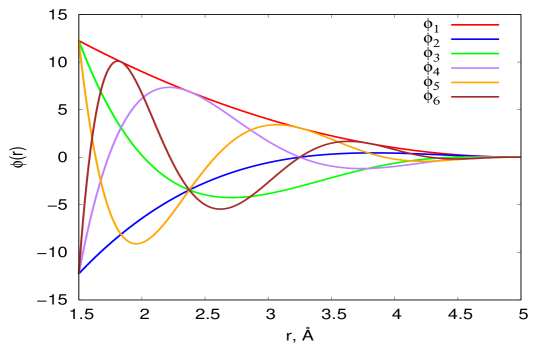
Figure 1: Radial basis $\varphi_{1},\ldots,\varphi_{6}$.

We construct our basis functions $B_{\alpha}$ as all possible contractions of the moment tensor descriptors (2) to scalar, e.g.:

$$B_{0}(\bm{r}_{i}) =M_{0,0}(\bm{r}_{i}),$$

$$B_{1}(\bm{r}_{i}) =(M_{1,2}(\bm{r}_{i})M_{0,1}(\bm{r}_{i}))\cdot M_{1,1}(\bm{r}_{i}),$$

$$B_{2}(\bm{r}_{i}) =M_{0,2}(\bm{r}_{i}):M_{2,2}(\bm{r}_{i}),$$

$$...$$

where “$\cdot$” is the dot product, “:” is the Frobenius product, $M_{0,0}(\bm{r}_{i})$ is a scalar ($\nu=0$), $M_{0,1}(\bm{r}_{i})$ and $M_{1,1}(\bm{r}_{i})$ are vectors ($\nu=1$), while $M_{0,2}(\bm{r}_{i})$, $M_{1,2}(\bm{r}_{i})$ and $M_{2,2}(\bm{r}_{i})$ are matrices ($\nu=2$). We denote the free parameters of MTP by ${\bm{\theta}}^{\rm MTP}:=(\xi_{\alpha},c^{(\beta)}_{\mu,z_{i},z_{j}})$. The total interaction energy is $E^{\rm MTP}=E({\bm{\theta}}^{\rm MTP};\bm{x})=\sum_{i=1}^{n}V^{\rm MTP}_{i}$.

Next we describe the QEq model. This model was proposed in [14] and we use it in the following form:

$$\displaystyle E^{\rm QEq} :=E(\bm{\theta}^{\rm QEq};\bm{x},\bm{q})=\sum_{i=1}^{n}\Bigl{(}\chi_{z_{i}}q_{i}+\dfrac{J_{z_{i}}q_{i}^{2}}{2}+\sum_{j<i}\dfrac{q_{i}q_{j}}{|r_{ij}|}\Bigr{)},$$ (4)

where $\chi_{z_{i}}$ is the electronegativity of the atom of type $z_{i}$, $J_{z_{i}}$ describes repulsion between two electrons, $q_{i}$ and $q_{j}$ are the partial charges of the $i$-th and the $j$-th atom, respectively. The third sum in (4) describing the Coulombic interaction converges only conditionally, therefore we use the Ewald summation [54] for its calculation. We denote the free parameters of the QEq model by ${\bm{\theta}}^{\rm QEq}:=(\chi_{z_{i}},J_{z_{i}})$ and the collection of partial charges in a configuration by $\bm{q}:=(q_{1},\ldots,q_{n})$. It should be emphasized that (4) is a long-range interaction model with no cutoff radius.

We find the partial charges $q_{i}$ by solving the following optimization problem for each configuration $\bm{x}$ occurring in a simulation:

$$\begin{array}[]{c}\displaystyle\bm{q}^{*}=\underset{\bm{q}}{\operatorname{arg\,min}}\,E(\bm{\theta}^{\rm QEq};\bm{x},\bm{q})\\ \displaystyle\mbox{subject to}\leavevmode\nobreak\ \sum_{i=1}^{n}q_{i}=0.\end{array}$$ (5)

This expresses equilibration of charges, see [14] for details.

The second interatomic interaction model used in this work is, thus, the combination of the MTP and the QEq model:

$$E^{\rm MTP+QEq}:=E(\bm{\theta}^{\rm MTP+QEq};\bm{x},\bm{q})=E({\bm{\theta}}^{\rm MTP};\bm{x})+E(\bm{\theta}^{\rm QEq};\bm{x},\bm{q}),$$ (6)

where $\bm{\theta}^{\rm MTP+QEq}:=({\bm{\theta}}^{\rm MTP},{\bm{\theta}}^{\rm QEq})$.

2.2 Fitting

We now describe the optimization problems for finding the free parameters of the models described above. Let us consider a training set which consists of $K$ configurations $\bm{x}^{(k)}$ ($k=1,\ldots,K$). Suppose also that we have the DFT energies $E^{{\rm DFT},(k)}$, forces $\bm{f}^{{\rm DFT},(k)}$, and stresses $\bm{\sigma}^{{\rm DFT},(k)}$, where by $\bm{f}^{{\rm DFT},(k)}$ we mean the collection of forces on each atom of the $k$-th configuration and by $\bm{\sigma}^{{\rm DFT},(k)}$ the collection of stresses of the $k$-th configuration. In order to find the free parameters of the MTP we solve the following optimization problem:

$$\begin{array}[]{r@{}l}\displaystyle L({\bm{\theta}}^{\rm MTP})=\sum_{k=1}^{K}\Bigl{[}&w_{\rm e}\left(E^{{\rm DFT},(k)}-E({\bm{\theta}}^{\rm MTP};\bm{x}^{(k)})\right)^{2}\\ \displaystyle\hfil&+w_{\rm f}\sum_{i}\left|f^{{\rm DFT},(k)}_{i}-f_{i}({\bm{\theta}}^{\rm MTP};\bm{x}^{(k)})\right|^{2}\\ \displaystyle\hfil&+w_{\rm s}\sum_{i,j=1}^{3}\left(\sigma^{{\rm DFT},(k)}_{ij}-\sigma_{ij}({\bm{\theta}}^{\rm MTP};\bm{x}^{(k)})\right)^{2}\Bigr{]}\to\operatorname{min},\end{array}$$ (7)

where $w_{\rm e}$, $w_{\rm f}$ and $w_{\rm s}$ are some nonnegative weights. We solve a similar problem in order to find the MTP parameters.

Because of partial charges in the combined model (6) we apply a slightly different algorithm for finding the free parameters of MTP+QEq. Before each iteration of minimizing the objective function

$$\begin{array}[]{r@{}l}\displaystyle L({\bm{\theta}}^{\rm MTP+QEq})=\sum_{k=1}^{K}\Bigl{[}&w_{\rm e}\left(E^{{\rm DFT},(k)}-E({\bm{\theta}}^{\rm MTP+QEq};\bm{x}^{(k)},\bm{q}^{*,(k)})\right)^{2}\\ \displaystyle\hfil&+w_{\rm f}\sum_{i=1}^{N^{(k)}}\left|f^{{\rm DFT},(k)}_{i}-f_{i}({\bm{\theta}}^{\rm MTP+QEq};\bm{x}^{(k)},\bm{q}^{*,(k)})\right|^{2}\\ \displaystyle\hfil&+w_{\rm s}\sum_{i,j=1}^{3}\left(\sigma^{{\rm DFT},(k)}_{ij}-\sigma_{ij}({\bm{\theta}}^{\rm MTP+QEq};\bm{x}^{(k)},\bm{q}^{*,(k)})\right)^{2}\Bigr{]}\to\operatorname{min},\end{array}$$ (8)

we optimize the charges $q^{*,(k)}$ for each configuration by solving the problem (5). Thus, we have different equilibrated charges $q^{*,(k)}$ during each iteration of solving (8).

Since the models depend nonlinearly on the parameters $\bm{\theta}$, we use a quasi-Newton optimization method, namely, the Broyden–Fletcher–Goldfarb–Shanno algorithm (BFGS). To that end, we explicitly implemented the gradients of the loss function with respect to the parameters $\bm{\theta}$ for each of the methods. In particular, for MTP, we have implemented an efficient back-propagation algorithm which has a favorable scaling when the number of parameters is large.

2.3 Uncertainty quantification

The fitted potential is a random quantity: it depends on the random training set and/or a particular local minimum that the optimization routine has found. Therefore the predictions of such potentials are also, strictly speaking, random. In order to quantify such randomness (uncertainty), we fit an ensemble of potentials of each type starting from random initial values of parameters and analyze the distribution of predictions by each type of potential, not just a single value of the “best” potential. In particular, we analyze the standard deviation (sometimes called predictive variance) of predictions of the ensemble of potentials and compare it to the actual error. As we will see, in our tests the standard deviation gives a good estimation of the actual error in all the quantities of interest considered in this study. Such technique of estimating the uncertainty of predictions is known as query by committee [55].

3 Numerical Testing

We fit two potentials, MTP and MTP+QEq, and test how well they predict the elastic constants, VFE, phonon spectrum, and RDFs of the $\alpha$-quartz SiO₂. $\alpha$-quartz is the stable crystalline structure of SiO₂ at normal temperature and pressure.

3.1 Training dataset

We composed the training dataset by perturbing and introducing defects to the $\alpha$-quartz SiO₂. This structure has a trigonal unit cell with the lattice parameters $a=b=5.022\leavevmode\nobreak\ \mbox{\AA}$, $c=5.551\leavevmode\nobreak\ \mbox{\AA}$, $\alpha=\beta=90^{\circ}$, and $\gamma=120^{\circ}$. The unit cell contains 3 atoms of silicon and 6 atoms of oxygen.

We first generated 22 (all possible) supercells with 9, 18, 27 and 36 atoms by replicating the unit cell in different axes and applying shear. Next, in addition to pristine crystals, we generated a number of structures with a single O-vacancy defects, which were then relaxed (equilibrated). We used the VASP code [56, 57, 58, 59] for DFT calculations with the PBE functional [60], the PAW pseudopotentials [61], k-point meshes were equivalent to the $4\times 4\times 3$ k-point mesh in the unit cell and a cutoff energy was 400 eV. After the configurations were relaxed, we randomly displaced every atom in each configuration by about $0.1\leavevmode\nobreak\ \mbox{\AA}$. From each “undisplaced” configuration several configurations with displaced atoms were generated. In addition, in order to predict elastic constants, we added 13 more configurations to the training dataset: 12 of them are relaxed configurations without atomic defects and with lattice vectors extended, compressed, or sheared by 2%, i.e., two configurations with extensions/compressions along each of six directions ($xx$, $yy$, $zz$, $yz$, $xz$, $xy$) and one of them is the relaxed configuration without any defects and extensions/compressions of lattice vectors. Thus, our dataset contains 418 SiO₂ atomic configurations with oxygen vacancies, random displacements of atomic positions and shear/compression.

3.2 Comparison of Potentials

We fit two types of potentials: MTP (1) and MTP+QEq (6). For all the potentials we choose $R_{\rm min}=1.4\,\mbox{\AA}$, $R_{\rm cut}=5\,\mbox{\AA}$, and eight radial functions (3). We consider the MTPs with 9, 29 and 92 basis functions $B_{\alpha}$. We denote these potentials by MTP₁, MTP₂ and MTP₃, respectively. The total number of free parameters in these potentials are 150, 250, and 500, respectively. MTPs in the MTP+QEq models contain 9 and 29 basis functions, thus we consider MTP₁+QEq and MTP₂+QEq models. The weights in the objective functions (7), (8) were $w_{\rm e}=1$, $w_{\rm f}=10^{-2}\,\mbox{\AA}^{2}$, and $w_{\rm s}=10^{-3}$.

Potential	energy error	force error	stress error	Si partial charge
	meV/atom	meV/Å (%)	GPa ($\%$)	in ideal crystal
MTP1	2.66 $\pm$ 0.14	202.3 $\pm$ 7.8	0.32 $\pm$ 0.04	-
		(11.0 $\pm$ 0.4%)	(13.6 $\pm$ 1.7%)
MTP1+QEq	2.71 $\pm$ 0.42	206.2 $\pm$ 20.7	0.29 $\pm$ 0.01	0.57 $\pm$ 0.11
		(11.1 $\pm$ 1.1%)	(12.3 $\pm$ 0.5%)
MTP2	1.87 $\pm$ 0.11	141.5 $\pm$ 7.0	0.20 $\pm$ 0.02	-
		(7.7 $\pm$ 0.4%)	(8.3 $\pm$ 0.9%)
MTP2+QEq	1.96 $\pm$ 0.18	146.0 $\pm$ 11.8	0.21 $\pm$ 0.03	0.66 $\pm$ 0.11
		(8.0 $\pm$ 0.6%)	(8.9 $\pm$ 1.1%)
MTP3	1.70 $\pm$ 0.08	130.5 $\pm$ 5.6	0.17 $\pm$ 0.01	-
		(7.1 $\pm$ 0.3%)	(7.3 $\pm$ 0.6%)

Table 1: Comparison of the average absolute and relative training root-mean-square errors and their standard deviations for the five ensembles of models on the same dataset. In the last column the average silicon partial charge in the ideal $\alpha$-quartz crystal and its standard deviation are shown. MTP and MTP+QEq models with the same number of basis functions have similar accuracy. Increase in the number of basis functions in MTP improves the accuracy, whereas adding QEq to MTP does not.

For each model type we fit an ensemble of five potentials in order to be able to estimate uncertainty due to randomness of the fitting. We have manually verified that in each ensemble all five potentials converged to a different minimum. The average fitting errors and the standard deviations for each family of potentials are reported in Table 1. We trained five ensembles of potentials: MTP₁, MTP₂, MTP₃, MTP₁+QEq and MTP₂+QEq. Each ensemble includes five potentials. We can see that MTP and MTP+QEq with the same number of basis functions have rather close training errors and, thus, adding QEq to MTP does not improve the accuracy. On the other hand, the increase in the number of functions $B_{\alpha}$ in MTP improves the accuracy and reduces the deviation in errors within an ensemble of potentials. In other words, judging by training errors alone, adding more basis functions to the potential improves the accuracy, but adding the QEq model does not.

In order to check the predictive power of the potentials we compared average elastic constants, VFEs, phonon spectra and RDFs calculated by these potentials to the results computed with DFT.

	DFT	MTP1			MTP1+QEq			MTP2			MTP2+QEq			MTP3
C11	91.1	82.2	$\pm$	21.5	104.1	$\pm$	4.4	96.7	$\pm$	16.9	94.8	$\pm$	11.9	88.5	$\pm$	9.2
C12	5.9	1.5	$\pm$	15.8	23.7	$\pm$	5.2	12.1	$\pm$	13.5	1.2	$\pm$	11.3	1.2	$\pm$	13.1
C13	16.0	14.0	$\pm$	13.2	33.9	$\pm$	7.2	20.2	$\pm$	10.1	5.2	$\pm$	15.2	8.4	$\pm$	10.0
C14	15.8	13.7	$\pm$	4.1	10.0	$\pm$	1.6	13.7	$\pm$	4.2	14.4	$\pm$	3.7	18.7	$\pm$	4.5
C33	93.8	89.2	$\pm$	13.7	108.7	$\pm$	11.9	97.7	$\pm$	14.4	83.4	$\pm$	22.1	87.8	$\pm$	8.9
C44	53.2	59.6	$\pm$	7.0	63.9	$\pm$	4.1	61.2	$\pm$	5.9	62.5	$\pm$	2.6	54.5	$\pm$	6.2
C66	42.6	40.3	$\pm$	3.0	39.6	$\pm$	1.8	42.3	$\pm$	5.0	46.5	$\pm$	1.2	43.6	$\pm$	3.7
bias		5.0			13.0			4.9			7.2			4.4
UE				12.8			6.1			11.0			12.0			8.5

Table 2: Average elastic constants of SiO₂ $\alpha$-quartz (in GPa) calculated by DFT, MTPs and MTP+QEq models, and their standard deviations due to randomness in fitting. Bias is the root-mean-square deviation of the average predicted elastic constants from the reference DFT results. The last line shows the root-mean-square standard deviations (uncertainty estimate, UE) of the predictions. The errors in the average elastic constants prediction reduce while the number of basis functions in MTP increases. Adding QEq to MTP worsens the accuracy of elastic constants prediction, but the uncertainty in quantification is either close (MTP₂+QEq) or better (MTP₁+QEq) to the ones calculated on the plain MTPs.

The average elastic constants and their standard deviations for three ensembles of MTPs and two ensembles of MTP+QEq models are given in Table 2 together with their root-mean-square error compared to the reference DFT values (bias) and root-mean-square standard deviation (uncertainty due to randomness in the fitting). One can see that the errors in the average elastic constants reduce as the number of basis functions in MTP increases. The combination of MTP and QEq yields even worse elastic constants as compared to the plain MTP with the same number of basis functions.

	DFT	MTP1			MTP1+QEq			MTP2			MTP2+QEq			MTP3
VFE	2.23	1.85	$\pm$	0.25	1.69	$\pm$	0.23	2.00	$\pm$	0.12	1.96	$\pm$	0.19	2.13	$\pm$	0.02
Bias		0.38			0.54			0.23			0.27			0.10

Table 3: Average vacancy formation energies (eV) of SiO₂ $\alpha$-quartz as calculated by the ensembles of MTPs and MTP+QEq models, their standard deviations. In the last line the absolute errors (eV) in vacancy formation energy calculations (biases) are presented. MTP₁ and MTP₁+QEq as well as MTP₂ and MTP₂+QEq gave close average VFEs, the uncertainty in predictions of the VFEs reduces and the accuracy of the VFEs calculation improves while increasing the number of basis functions.

In order to obtain the average VFEs and their standard deviations we relaxed and calculated the energies of two configurations: the first configuration is the $2\times 2\times 2$ supercell of 72 atoms and the second configuration is the same supercell with the oxygen atom vacancy. The average VFEs and their standard deviations calculated by the five ensembles of potentials and the reference DFT VFE are presented in Table 3. The findings are similar to those for elastic constants: MTP₁ and MTP₁+QEq as well as MTP₂ and MTP₂+QEq gave close average VFEs, the uncertainty in predictions of the VFEs reduces and the accuracy of the VFEs calculation improves with increasing the number of $B_{\alpha}$.

Next we test how well the potentials reproduce the phonon spectrum. Again, we compare average phonon spectra to the reference DFT spectrum, i.e., we take the averaged phonon spectrum for each ensemble of potentials rather than one spectrum from one potential. We used the PHONOPY open-source package [62] to plot the spectra. The results shown in Figure 2 were obtained with the $4\times 4\times 4$ supercell of the nine-atom primitive unit cell. The k-path for this system was $\Gamma$-M-K-$\Gamma$-A-L-H-A$|$L-M$|$K-H (see, e.g., [63]), where $\Gamma$, M, K, A, L and H are the high-symmetry points in the Brillouin zone. Each ensemble of potentials, generally, shows a good agreement with the reference DFT data except for the very high frequencies, but, as it was expected, MTP₁ and MTP₁+QEq appear to be the least accurate among all the ensembles of potentials, and adding QEq to MTP does not improve the spectrum.

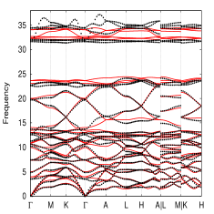
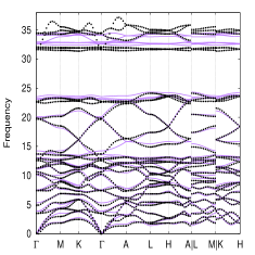
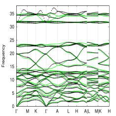
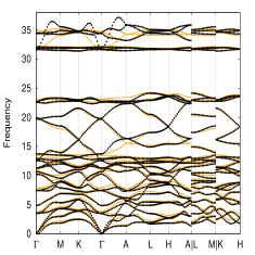
Figure 2: Phonon spectra of SiO₂ $\alpha$-quartz predicted by MTP₁, MTP₁+QEq, MTP₂, MTP₂+QEq and MTP₃ (the figures (a), (b), (c), (d), and (e), respectively) compared to the reference DFT phonon spectrum (black circles). Each ensemble of potentials, generally, shows a good agreement with the reference DFT data except for the very high frequencies. MTP₁ and MTP₁+QEq appear to be least accurate among all the ensembles of potentials, adding QEq to MTP does not improve the spectrum.

Finally, we compare the radial distribution functions. The RDF calculations were performed in a $2\times 2\times 2$ supercell with 72 atoms. To obtain the RDFs for the five ensembles of potentials we ran molecular dynamics on LAMMPS [64] sampling an NVT ensemble with $T=300\,$K and time step of 1 fs. The reference RDFs were obtained by running molecular dynamics on VASP. The RDFs are plotted in Figure 3. MTP₃ showed the best correspondence with the reference RDFs, this is the only potential which correctly described all the peaks of O-O RDF. RDFs predicted with MTP₁ have the worst agreement with the reference RDFs among all the ensembles of the potentials, the rest three potentials have demonstrated the close accuracy to each other in description of the DFT RDFs.

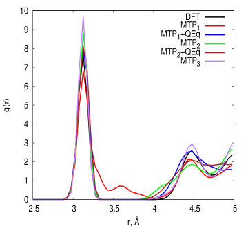
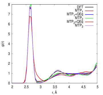
Figure 3: Radial distribution function (a) for Si–Si, and (b) O–O, computed at $T=300$ K. MTP₃ is in the best agreement with DFT, MTP₁ has the worst correspondence to the reference RDFs, the results of the rest three models are close to each other.

4 Conclusion

In this work we investigated two strategies for improving the accuracy of a machine-learning interatomic potential, namely adding more fitting parameters to it and adding a charge-equilibration model to it. To that end we tested the MTP potentials [22, 23, 24] with increasing number of fitting parameters and MTP combined with the charge-equilibration model (MTP+QEq). In order to make a meaningful comparison we assessed the uncertainty of predictions of each potential. The uncertainty was due to the fact that typically the parameters of the fitted potentials are only near a local optimum, and an optimization routine typically finds some random local optimum. Our conclusion is that adding more parameters to MTP does improve its predictive accuracy and reduces uncertainty of its predictions, whereas supplementing MTP with a charge-equilibration model does not reduce the error and often increases the uncertainty of the predictions. We thus conclude that the QEq model could not, at least in a straightforward manner (i.e., by local optimization of model parameters), improve machine-learning potentials.

5 Acknowledgements

The authors thank our colleague, Konstantin Gubaev, for giving advance access to the code implementing MTP. I.N. also thanks Dmitry Aksenov for valuable advices concerning the usage of DFT (VASP) and application of PHONOPY to the computations of phonon spectra. The work was supported by the Russian Science Foundation (grant number 18-13-00479).

6 Data availability

The data used for the fitting of the interatomic potentials are available to download from http://gitlab.skoltech.ru/Novikov/SiO2_training_set.

References

- [1] P. F. Satterthwaite, A. G. Scheuermann, P. K. Hurley, C. E. Chidsey, P. C. McIntyre, Engineering interfacial silicon dioxide for improved metal–insulator–semiconductor silicon photoanode water splitting performance, ACS applied materials & interfaces 8 (20) (2016) 13140–13149.
- [2] T. R. Rao, Metal casting: Principles and practice, New Age International, 2007.
- [3] Z. H. Stachurski, Fundamentals of amorphous solids: structure and properties, John Wiley & Sons, 2015.
- [4] L. Levien, C. T. Prewitt, D. J. Weidner, Structure and elastic properties of quartz at pressure, American Mineralogist 65 (9-10) (1980) 920–930.
- [5] D. Strauch, B. Dorner, Lattice dynamics of alpha-quartz. i. experiment, Journal of Physics: Condensed Matter 5 (34) (1993) 6149.
- [6] R. Ghita, C. Logofatu, C.-C. Negrila, F. Ungureanu, C. Cotirlan, A.-S. Manea, M.-F. Lazarescu, C. Ghica, Study of SiO2/Si interface by surface techniques, in: Crystalline Silicon-Properties and Uses, InTech, 2011.
- [7] T. Watanabe, H. Fujiwara, H. Noguchi, T. Hoshino, I. Ohdomari, Novel interatomic potential energy function for Si, O mixed systems, Japanese journal of applied physics 38 (4A) (1999) L366.
- [8] P. Ganster, G. Tréglia, A. Saúl, Atomistic modeling of strain and diffusion at the Si/SiO2 interface, Physical Review B 81 (4) (2010) 045315.
- [9] S. R. Billeter, A. Curioni, D. Fischer, W. Andreoni, Ab initio derived augmented tersoff potential for silicon oxynitride compounds and their interfaces with silicon, Physical Review B 73 (15) (2006) 155329.
- [10] D. t. Williams, S. Cox, Nonbonded potentials for azahydrocarbons: the importance of the coulombic interaction, Acta Crystallographica Section B 40 (4) (1984) 404–417.
- [11] B. Van Beest, G. J. Kramer, R. Van Santen, Force fields for silicas and aluminophosphates based on ab initio calculations, Physical Review Letters 64 (16) (1990) 1955.
- [12] P. Tangney, S. Scandolo, An ab initio parametrized interatomic force field for silica, The Journal of chemical physics 117 (19) (2002) 8898–8904.
- [13] J. Kermode, S. Cereda, P. Tangney, A. De Vita, A first principles based polarizable O (N) interatomic force field for bulk silica, The Journal of Chemical Physics 133 (9) (2010) 094102.
- [14] A. K. Rappe, W. A. Goddard III, Charge equilibration for molecular dynamics simulations, The Journal of Physical Chemistry 95 (8) (1991) 3358–3363.
- [15] A. Yasukawa, Using an extended tersoff interatomic potential to analyze the static-fatigue strength of SiO2 under atmospheric influence, JSME international journal. Ser. A, Mechanics and material engineering 39 (3) (1996) 313–320.
- [16] A. C. Van Duin, A. Strachan, S. Stewman, Q. Zhang, X. Xu, W. A. Goddard, Reaxffsio reactive force field for silicon and silicon oxide systems, The Journal of Physical Chemistry A 107 (19) (2003) 3803–3811.
- [17] J. Yu, S. B. Sinnott, S. R. Phillpot, Charge optimized many-body potential for the Si/SiO2 system, Physical Review B 75 (8) (2007) 085311.
- [18] J. Behler, M. Parrinello, Generalized neural-network representation of high-dimensional potential-energy surfaces, Physical review letters 98 (14) (2007) 146401.
- [19] A. P. Bartók, M. C. Payne, R. Kondor, G. Csányi, Gaussian approximation potentials: The accuracy of quantum mechanics, without the electrons, Physical review letters 104 (13) (2010) 136403.
- [20] W. J. Szlachta, A. P. Bartók, G. Csányi, Accuracy and transferability of gaussian approximation potential models for tungsten, Physical Review B 90 (10) (2014) 104108.
- [21] J. R. Boes, M. C. Groenenboom, J. A. Keith, J. R. Kitchin, Neural network and reaxff comparison for au properties, International Journal of Quantum Chemistry 116 (13) (2016) 979–987.
- [22] A. V. Shapeev, Moment tensor potentials: A class of systematically improvable interatomic potentials, Multiscale Modeling & Simulation 14 (3) (2016) 1153–1173.
- [23] K. Gubaev, E. V. Podryabinkin, A. V. Shapeev, Machine learning of molecular properties: Locality and active learning, The Journal of Chemical Physics 148 (24) (2018) 241727.
- [24] K. Gubaev, E. V. Podryabinkin, G. L. Hart, A. V. Shapeev, Accelerating high-throughput searches for new alloys with active learning of interatomic potentials, Computational Materials Science 156 (2019) 148–156.
- [25] N. Artrith, A. M. Kolpak, Grand canonical molecular dynamics simulations of Cu–Au nanoalloys in thermal equilibrium using reactive ANN potentials, Comput. Mater. Sci. 110 (2015) 20–28.
- [26] J. Behler, Neural network potential-energy surfaces in chemistry: a tool for large-scale simulations, Phys. Chem. Chem. Phys. 13 (40) (2011) 17930–17955.
-
[27]
J. Behler, Representing
potential energy surfaces by high-dimensional neural network potentials, J.
Phys. Condens. Matter. 26 (18) (2014) 183001.
URL http://stacks.iop.org/0953-8984/26/i=18/a=183001 - [28] P. E. Dolgirev, I. A. Kruglov, A. R. Oganov, Machine learning scheme for fast extraction of chemically interpretable interatomic potentials, AIP Advances 6 (8) (2016) 085318.
- [29] M. Gastegger, P. Marquetand, High-dimensional neural network potentials for organic reactions and an improved training algorithm, J. Chem. Theory Comput. 11 (5) (2015) 2187–2198.
- [30] S. Manzhos, R. Dawes, T. Carrington, Neural network-based approaches for building high dimensional and quantum dynamics-friendly potential energy surfaces, Int. J. Quantum Chem. 115 (16) (2015) 1012–1020.
- [31] S. K. Natarajan, T. Morawietz, J. Behler, Representing the potential-energy surface of protonated water clusters by high-dimensional neural network potentials, Phys. Chem. Chem. Phys. 17 (13) (2015) 8356–8371.
-
[32]
N. Lubbers, J. S. Smith, K. Barros,
Hierarchical modeling of molecular
energies using a deep neural network, J. Chem. Phys. 148 (24) (2018) 241715.
doi:10.1063/1.5011181.
URL https://doi.org/10.1063/1.5011181 -
[33]
J. S. Smith, O. Isayev, A. E. Roitberg,
ANI-1: an extensible neural
network potential with DFT accuracy at force field computational cost,
Chem. Sci. 8 (4) (2017) 3192–3203.
doi:10.1039/c6sc05720a.
URL https://doi.org/10.1039/c6sc05720a -
[34]
B. Kolb, L. C. Lentz, A. M. Kolpak,
Discovering charge density
functionals and structure-property relationships with PROPhet: A general
framework for coupling machine learning and first-principles methods, Sci.
Rep. 7 (1).
doi:10.1038/s41598-017-01251-z.
URL https://doi.org/10.1038/s41598-017-01251-z -
[35]
V. L. Deringer, G. Csányi,
Machine learning
based interatomic potential for amorphous carbon, Phys. Rev. B 95 (2017)
094203.
doi:10.1103/PhysRevB.95.094203.
URL https://link.aps.org/doi/10.1103/PhysRevB.95.094203 - [36] V. L. Deringer, C. J. Pickard, G. Csányi, Data-driven learning of total and local energies in elemental boron, Phys. Rev. Lett. 120 (15) (2018) 156001.
- [37] A. Grisafi, D. M. Wilkins, G. Csányi, M. Ceriotti, Symmetry-adapted machine learning for tensorial properties of atomistic systems, Phys. Rev. Lett. 120 (3) (2018) 036002.
-
[38]
A. Thompson, L. Swiler, C. Trott, S. Foiles, G. Tucker,
Spectral
neighbor analysis method for automated generation of quantum-accurate
interatomic potentials, J. Comput. Phys. 285 (2015) 316 – 330.
doi:http://dx.doi.org/10.1016/j.jcp.2014.12.018.
URL http://www.sciencedirect.com/science/article/pii/S0021999114008353 - [39] V. Botu, R. Ramprasad, Learning scheme to predict atomic forces and accelerate materials simulations, Phys. Rev. B 92 (9) (2015) 094306.
-
[40]
Z. Li, J. R. Kermode, A. De Vita,
Molecular
dynamics with on-the-fly machine learning of quantum-mechanical forces,
Phys. Rev. Lett. 114 (2015) 096405.
doi:10.1103/PhysRevLett.114.096405.
URL http://link.aps.org/doi/10.1103/PhysRevLett.114.096405 - [41] I. Kruglov, O. Sergeev, A. Yanilkin, A. R. Oganov, Energy-free machine learning force field for aluminum, Sci. Rep. 7 (1) (2017) 8512.
- [42] K. Schütt, P.-J. Kindermans, H. E. S. Felix, S. Chmiela, A. Tkatchenko, K.-R. Müller, Schnet: A continuous-filter convolutional neural network for modeling quantum interactions, in: Advances in Neural Information Processing Systems, 2017, pp. 992–1002.
- [43] N. Artrith, T. Morawietz, J. Behler, High-dimensional neural-network potentials for multicomponent systems: Applications to zinc oxide, Physical Review B 83 (15) (2011) 153101.
- [44] B. Nebgen, N. Lubbers, J. S. Smith, A. E. Sifain, A. Lokhov, O. Isayev, A. E. Roitberg, K. Barros, S. Tretiak, Transferable dynamic molecular charge assignment using deep neural networks, Journal of chemical theory and computation 14 (9) (2018) 4687–4698.
- [45] M. Rupp, A. Tkatchenko, K.-R. Müller, O. A. Von Lilienfeld, Fast and accurate modeling of molecular atomization energies with machine learning, Physical review letters 108 (5) (2012) 058301.
- [46] H. Huo, M. Rupp, Unified representation for machine learning of molecules and crystals, preprint.
- [47] J. C. Snyder, M. Rupp, K. Hansen, K.-R. Müller, K. Burke, Finding density functionals with machine learning, Physical review letters 108 (25) (2012) 253002.
- [48] S. De, A. P. Bartók, G. Csányi, M. Ceriotti, Comparing molecules and solids across structural and alchemical space, Physical Chemistry Chemical Physics 18 (20) (2016) 13754–13769.
- [49] F. Faber, L. Hutchison, B. Huang, J. Gilmer, S. Schoenholz, G. Dahl, O. Vinyals, S. Kearnes, P. Riley, O. von Lilienfeld, Fast machine learning models of electronic and energetic properties consistently reach approximation errors better than dft accuracy, arXiv preprint arXiv:1702.05532.
- [50] K. Hansen, F. Biegler, R. Ramakrishnan, W. Pronobis, O. A. Von Lilienfeld, K.-R. Müller, A. Tkatchenko, Machine learning predictions of molecular properties: Accurate many-body potentials and nonlocality in chemical space, The journal of physical chemistry letters 6 (12) (2015) 2326–2331.
- [51] B. Huang, O. A. Von Lilienfeld, Communication: Understanding molecular representations in machine learning: The role of uniqueness and target similarity, Journal of Chemical Physics 145 (16).
- [52] J. Gilmer, S. S. Schoenholz, P. F. Riley, O. Vinyals, G. E. Dahl, Neural message passing for quantum chemistry, arXiv preprint arXiv:1704.01212.
- [53] K. T. Schütt, F. Arbabzadah, S. Chmiela, K. R. Müller, A. Tkatchenko, Quantum-chemical insights from deep tensor neural networks, Nature communications 8 (2017) 13890.
- [54] P. P. Ewald, Die berechnung optischer und elektrostatischer gitterpotentiale, Annalen der physik 369 (3) (1921) 253–287.
- [55] B. Settles, Active learning, Synthesis Lectures on Artificial Intelligence and Machine Learning 6 (1) (2012) 1–114.
- [56] G. Kresse, J. Hafner, Ab initio molecular dynamics for liquid metals, Physical Review B 47 (1) (1993) 558.
- [57] G. Kresse, J. Hafner, Ab initio molecular-dynamics simulation of the liquid-metal–amorphous-semiconductor transition in germanium, Physical Review B 49 (20) (1994) 14251.
- [58] G. Kresse, J. Furthmüller, Efficiency of ab-initio total energy calculations for metals and semiconductors using a plane-wave basis set, Computational materials science 6 (1) (1996) 15–50.
- [59] G. Kresse, J. Furthmüller, Efficient iterative schemes for ab initio total-energy calculations using a plane-wave basis set, Physical review B 54 (16) (1996) 11169.
- [60] J. P. Perdew, K. Burke, M. Ernzerhof, Generalized gradient approximation made simple, Physical review letters 77 (18) (1996) 3865.
- [61] P. E. Blöchl, Projector augmented-wave method, Physical review B 50 (24) (1994) 17953.
- [62] A. Togo, I. Tanaka, First principles phonon calculations in materials science, Scripta Materialia 108 (2015) 1–5.
- [63] A. Jain, S. P. Ong, G. Hautier, W. Chen, W. D. Richards, S. Dacek, S. Cholia, D. Gunter, D. Skinner, G. Ceder, et al., Commentary: The materials project: A materials genome approach to accelerating materials innovation, Apl Materials 1 (1) (2013) 011002.
- [64] S. Plimpton, Fast parallel algorithms for short-range molecular dynamics, Journal of computational physics 117 (1) (1995) 1–19.