Epidemic spreading on time-varying multiplex networks

Abstract

Social interactions are stratified in multiple contexts and are subject to complex temporal dynamics. The systematic study of these two features of social systems has started only very recently mainly thanks to the development of multiplex and time-varying networks. However, these two advancements have progressed almost in parallel with very little overlap. Thus, the interplay between multiplexity and the temporal nature of connectivity patterns is poorly understood. Here, we aim to tackle this limitation by introducing a time-varying model of multiplex networks. We are interested in characterizing how these two properties affect contagion processes. To this end, we study SIS epidemic models unfolding at comparable time-scale respect to the evolution of the multiplex network. We study both analytically and numerically the epidemic threshold as a function of the overlap between, and the features of, each layer. We found that, the overlap between layers significantly reduces the epidemic threshold especially when the temporal activation patterns of overlapping nodes are positively correlated. Furthermore, when the average connectivity across layers is very different, the contagion dynamics are driven by the features of the more densely connected layer. Here, the epidemic threshold is equivalent to that of a single layered graph and the impact of the disease, in the layer driving the contagion, is independent of the overlap. However, this is not the case in the other layers where the spreading dynamics are sharply influenced by it. The results presented provide another step towards the characterization of the properties of real networks and their effects on contagion phenomena

Social interactions take place in different contexts and modes of communication. On a daily basis we interact at work, in the family and across a wide range of online platforms or tools, e.g. Facebook, Twitter, emails, mobile phones etc. In the language of modern Network Science, social networks can be conveniently modeled and described as multilayers networks ginestra18-1 ; kivela2014multilayer ; de2013mathematical ; boccaletti2014structure ; cozzo2018multiplex . This is not a new idea. Indeed, the concept of multiplexity to describe the stratification of interactions dates back several decades wasserman1994social ; verbrugge1979multiplexity ; doi:10.1086/228943 . However, the digitalization of our communications and the miniaturization of devices has just recently provided the data necessary to observe, at scale, and characterize the multilayer nature of social interactions.
As in the study of single layered networks, the research on multilayer graphs is divided in two interconnected areas. The first deals with the characterization of the structural properties of such entities boccaletti2014structure ; ginestra18-1 . One of the central observations is that the complex topology describing each type of interactions (i.e., each layer) might be different. Indeed, the set and intensity of interactions in different contexts (e.g., work, family etc..) or platforms (e.g., Facebook, Twitter etc..) is not the same. Nevertheless, we are present in some, if not all, these layers which are then coupled by different degrees of overlap. Another interesting feature of multilayer graphs is that the connectivity patterns in different layers might be topologically and temporally correlated starnini2017effects . The second area of research instead considers the function, such as sustaining diffusion or contagion processes, of multilayer networks ginestra18-1 ; de2016physics ; salehi2015spreading . A large fraction of this research aims at characterizing how the complex structural properties of multilayer graphs affect dynamical processes unfolding on their fabric. The first important observation is that disentangling connections in different layers, thus acknowledging multiplexity, gives raise to complex and highly non-trivial dynamics function of the interplay between inter and intra-layer connections gomez2013diffusion ; huang2018global ; bianconi2017epidemic ; osat2017optimal ; jiang2018resource ; granell2013dynamical ; massaro2014epidemic ; zhao2014multiple ; buono2014epidemics ; zhao2014immunization ; wang2014asymmetrically ; hu2014conditions ; cozzo2013contact . A complete summary of the main results in the literature is beyond the scope of the paper. We refer the interested reader to these recent resources for details ginestra18-1 ; kivela2014multilayer ; de2013mathematical ; boccaletti2014structure ; cozzo2018multiplex .
Despite the incredible growth of this area of Network Science over the last years, one particular aspect of multilayer networks is still largely unexplored: the interplay between multiplexity and the temporal nature of the connectivity patterns especially when dynamical processes unfolding on their fabric are concerned salehi2015spreading . This should not come as a surprise. Indeed, the systematic study of the temporal dynamics even in single layered graphs is very recent. In fact, the literature has been mostly focused on time-integrated properties of networks holme11-1 ; holme2015modern . As result, complex temporal dynamics acting at shorter time-scales have been traditionally discarded. However, the recent technological advances in data storing and collection are providing unprecedented means to probe also the temporal dimension of real systems. The access to this feature is allowing to discover properties of social acts invisible in time aggregated datasets, and is helping characterizing the microscopic mechanisms driving their dynamics at all time-scales perra12-1 ; karsai13-1 ; ubaldi2015asymptotic ; laurent2015calls ; moro10-1 ; clauset07 ; Isella:2011 ; saramaki2015seconds ; Saramaki21012014 ; Sekara06092016 . The advances in this arena are allowing to investigate the effects such temporal dynamics have on dynamical processes unfolding on time-varying networks. The study of the propagation of infectious diseases, idea, rumours, or memes etc.. on temporal graphs shows a rich and non trivial phenomenology radically different than what is observed on their static or annealed counter parts barrat2015face ; perra12-2 ; perra12-1 ; ribeiro12-2 ; PhysRevLett.112.118702 ; PhysRevE.87.032805 ; 10.1063 ; starnini13-1 ; starnini_rw_temp_nets ; valdano2015analytical ; scholtes2014causality ; Williams160196 ; rocha2014random ; takaguchi2012importance ; rocha2013bursts ; ghoshal2006attractiveness ; sun2015contrasting ; mistry2015committed ; pfitzner13-1 ; takaguchi12-1 ; takaguchi2013bursty ; holme2014birth ; holme2015basic ; wang2016statistical ; gonccalves2015social .
Before going any further, it is important to notice how in their more general form, multilayers networks, might be characterized by different types of nodes in each layers. For example, modern transportation systems in cities can be characterized as a multilayer network in which each layer captures a different transportation mode (tube, bus, public bikes etc..) and the links between layers connect stations (nodes) where people can switch mode of transport boccaletti2014structure ; de2016physics . A particular version of multilayer networks, called multiplex, is typically used in social networks. Here, the entities in each layers are of the same type (i.e., people). The inter-layer links are drawn only to connect the same person in different layers.
In this context, we introduce a model of time-varying multiplex networks. We aim to characterize the effects of temporal connectivity patterns and multiplexity on contagion processes. We model the intra-layer evolution of connections using the activity-driven framework perra12-1 . In this model of time-varying networks, nodes are assigned with an activity describing their propensity to engage in social interactions per unit time perra12-1 . Once active a node selects a partner to interact. Several selection mechanisms have been proposed, capturing different features of real social networks karsai13-1 ; ubaldi2015asymptotic ; ubaldi2016burstiness ; alessandretti2017random ; nadini2018epidemic . The simplest, that will be used here, is memoryless and random perra12-1 . The overlap between layers is modulated by a probability $p$. If $p=1$ all nodes are present in all layers. If $p=0$, the multiplex is formed by $M$ disconnected graphs. We consider $p$ as parameter and explore different regime of coupling between layers. Furthermore, each layer is characterized by an activity distribution. We consider different scenarios in which the activity of overlapping nodes (regulated by $p$) is uncorrelated and others in which is instead correlated. In these settings, we study the unfolding of Susceptible-Infected-Susceptible (SIS) epidemic processes keeling08-1 ; alex12-1 ; pastor2015epidemic . We derive analytically the epidemic threshold for two layers for any $p$ and any distributions of activities. In the limit of $p=1$ we find analytically the epidemic threshold for any number of layers. Interestingly, the threshold is a not trivial generalization of the correspondent quantity in the monoplex (single layer network). In the general case $0<p<1$ we found that the threshold is decreasing function of $p$. Positive correlations of overlapping nodes push the threshold to smaller values respect to the uncorrelated and negatively correlated cases. Furthermore, when the average connectivity of two layers is very different the critical behaviour of the system is driven by the more densely connected layer. In such scenario the epidemic threshold is not affected by the multiplexity, its value is equivalent to the case of a monoplex, and the overlap affects only the layer featuring the smaller average connectivity.
The paper is organized as follow. In Section I we introduce the multiplex model. In Section II we study first both analytically and numerically the spreading of SIS processes. Finally, in Section III we discuss our conclusions.

I Time-varying multiplex network model

We first introduce the multiplex model. For simplicity of discussion, we will consider the simplest case in which the system is characterized by $M=2$ layers $A$ and $B$. However, the same approach can be used to create a multiplex with any number of layers. Let us define $N$ as the total number of nodes in each layer. In general, we have three different categories of nodes: $N^{A}$, $N^{B}$ and $N^{o}$. They describe, respectively, the number of nodes that are present only in layer $A$, $B$, or in both. The last category is defined by a parameter $p$: the overlap between layers. Thus, on average, we have $N^{A}=N^{B}=(1-p)N$ and $N^{o}=pN$. As mentioned in the introduction, the temporal dynamics in each layer are defined by the activity-driven framework perra12-1 . Thus, each non-overlapping node is characterized by an activity extracted from a distribution $f_{A}(a)$ or $f_{B}(a)$ which captures its propensity to be engaged in a social interaction per unit time. Observations in real networks show that activity is typically heterogeneously distributed perra12-1 ; karsai13-1 ; ubaldi2015asymptotic ; ubaldi2016burstiness ; tomasello2014role ; ribeiro12-2 . Here, we assume that activities follow power-laws, thus $f_{\mathbf{x}}(a)=c_{\mathbf{x}}a^{-\gamma_{\mathbf{x}}}$ with $\mathbf{x}=[A,B]$ and $\epsilon\leq a\leq 1$ to avoid divergences. The overlapping nodes instead, are characterized by a joint activity distribution $h(a_{A},a_{B})$. As mentioned in the introduction, real multiplex networks are characterized by correlations across layers starnini2017effects . To account for such feature, we will consider three prototypical cases in which the activities of overlapping nodes in the two layers are i) uncorrelated ii) positively and iii) negatively correlated. To simplify the formulation and to avoid adding other parameters, in case of positive and negative correlations we adopt the following steps. We first extract the activities of the overlapping nodes from the two distributions $f_{\mathbf{x}}(a)$. Then we order them. In the case of positive correlation, a node that has the $r^{th}$ activity in $A$ will be assigned to the correspondent activity in $B$. In the case of negative correlations instead, a node that has the $r^{th}$ activity in $A$ will be assigned the $(pN-r+1)^{th}$ in $B$.

In these settings, the temporal evolution of the multiplex is defined as follow. For each realization, we randomly select $pN$ nodes as overlapping nodes between two layers. At each time step $t$:

• Each node is active with a probability defined by its activity.

• Each active node creates $m_{\mathbf{x}}$ links with randomly selected nodes. Multiple connections with the same node in the same layer within each time step are not allowed.

• Overlapping nodes can be active and create connections in both layers.

• At time step $t+\Delta t$ all connections are deleted and the process restart from the first point.

Connections have all the same duration of $\Delta t$. In the following, we set, without lack of generality, $\Delta t=1$. At each time the topology within each layer is characterized, mostly, by a set of disconnected stars of size $m_{\mathbf{x}}$. Thus, at the minimal temporal resolution each network looks very different than the static or annealed graphs we are used to see in the literature newman10-1 . However, it is possible to show that, integrating links over $T$ time steps in the limit in which $T\ll N$, the resulting network has a degree distribution that follows the activity perra12-1 ; starnini13-2 ; ubaldi2015asymptotic . This is qualitatively similar to what is observed in real temporal networks where the topological features at different time-scales are very different than the late (or time integrated) characteristics Sekara06092016 .
At each time step the average degree in each layer can be computed as:

$$\langle k\rangle^{\mathbf{x}}_{t}=\frac{2E^{\mathbf{x}}_{t}}{N}=2m_{\mathbf{x}}\left[(1-p)\langle a_{\mathbf{x}}\rangle+p\langle a_{\mathbf{x}}\rangle_{o}\right],$$ (1)

where $E^{\mathbf{x}}_{t}$ is the number of links generated in each layer at each time step. Furthermore, $\langle a_{\mathbf{x}}\rangle=\sum_{a}f_{\mathbf{x}}(a)a$ and $\langle a_{\mathbf{x}}\rangle_{o}=\sum_{a_{A}}\sum_{a_{B}}h(a_{A},a_{B})a_{\mathbf{x}}$ are the average activity of non-overlapping and overlapping nodes in each layer respectively. Similarly, the total average degree (often called overlapping degree battiston2014structural ), at each time step, is:

$$\langle k\rangle_{t}=\frac{2\sum\limits_{y\in\mathbf{x}}E^{y}_{t}}{2N-pN}=2\frac{\sum\limits_{y\in\mathbf{x}}m_{y}\left[(1-p)\langle a_{y}\rangle+p\langle a_{y}\rangle_{o}\right]}{(2-p)}.$$ (2)

Thus, the average connectivity, at each time step, is determined by the number of links created in each layer, and by the interplay between the average activity of overlapping and non-overlapping nodes. As shown in Figure 1 (top panel), Eq. 2 describes quite well the behaviour of the average overlapping degree which is an increasing function of $p$. Indeed, the larger the fraction of overlapping nodes, the larger the connectivity of such nodes across layers. As we will see in the next section, this feature affects significantly the unfolding on contagion processes.
In Figure 1 (bottom panel) we show the integrated degree distribution of the overlapping degree for different $p$. The plot clearly shows how the functional form is defined by the activity distributions of the two layers which in this case are equal. An increase in the fraction of overlapping nodes, does not change the distribution of the overlapping degree, it introduces a vertical shift which however is more visible for certain values of $k$.

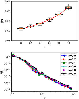
Figure 1: (Top panel) The average overlapping degree of the time-integrated multiplex networks as function of the fraction of the overlapping nodes, $p$. The red line is computed by Eq. (2). (Bottom panel) The distribution of the integrated overlapping degree for different $p$. Both in panels, the activities of the overlapping nodes in the two layers are uncorrelated. The exponents for the distributions of activities are $\gamma_{\mathbf{x}}=2.1$. The simulations are performed on networks of $10^{5}$ nodes with $m_{\mathbf{x}}=1$, integrated over $100$ time steps and averaged over 100 runs.

II Contagion processes

In order to understand how the interplay between multiplexity and temporal connectivity patterns affects dynamical processes, we consider SIS contagion phenomena spreading on the multiplex model introduced in the previous section. In this prototypical epidemic model each node can be in one of two compartments. Healthy nodes are susceptible to the disease and thus in the compartment $S$. Infectious nodes instead join the compartment $I$. The natural history of the disease is defined as follows. A susceptible, in contact with an infected node, might get sick and infectious with probability $\lambda$. Each infected node spontaneously recovers with rate $\mu$ thus staying infectious for $\mu^{-1}$ time steps, on average. One crucial feature of epidemic models is the threshold which determines the conditions above which a disease is able to affect a macroscopic fraction of the population keeling08-1 ; alex12-1 ; pastor2015epidemic . In case of SIS models, below the threshold the disease dies out reaching the so called disease-free equilibrium. Above threshold instead, the epidemic reaches an endemic stationary state. This can be captured running the simulations for longer times and thus estimating the fraction of infected nodes for $t\rightarrow\infty$: $i_{\infty}$. In general, in a multiplex network, such fraction might be different across layers. Thus, we can define: $i_{\infty}^{\mathbf{x}}$. To characterize the threshold we could study the behavior of such fraction(s) as function of $\lambda/\mu$. Indeed, the final number of infected nodes acts as order parameter in a second order phase transition alex12-1 . However, due to the stochastic nature of the process, the numerical estimation of the endemic state, especially in proximity of the threshold is not easy. Thus, we adopt another method measuring the life time of the process, $L$ boguna13-1 . This quantity is defined as the average time the disease needs either to die out or to infect a macroscopic fraction $Y$ of the population. The life time acts as the susceptibility in phase transition thus allows a more precise numerical estimation boguna13-1 .
In the case of single layer activity-driven networks, in which partners of interactions are chosen at random and without memory of past connections, the threshold can be written as (see Ref. perra12-1 for details):

$$\frac{\lambda}{\mu}>\frac{1}{m}\frac{1}{\langle a\rangle+\sqrt{\langle a^{2}\rangle}}.$$ (3)

Thus, the conditions necessary for the spread of the disease are set by the interplay between the features of the disease (left side) and the dynamical properties of the time-varying networks where the contagion unfolds (right side). The latter are regulated by first and second moment of the activity distribution and by the number of connections created by each active node (i.e., $m$). It is important to notice that Eq. 3 considers the case in which the time-scale describing the evolution of the connectivity patterns and the epidemic process are comparable. The contagion process is unfolding on a time-varying network. In the case when links are integrated over time and the SIS process spreads on a static or annealed version of the graph, the epidemic threshold will be much smaller morris93-1 ; morris95-1 ; perra12-1 . This is due to the concurrency of connections which favours the spreading. In this limit of time-scale separation between the dynamics of and on networks, the evolution of the connectivity patterns is considered either much slower (static case) or much faster (annealed case) respect to the epidemic process. In the following, we will only consider the case of comparable time-scales.
What is the threshold in the case of our multiplex and time-varying network model? In the limit $p=0$ the number of overlapping nodes is zero. The two layers are disconnected thus the system is characterized by two independent thresholds regulated by the activity distributions of the two layers. The most interesting question, is then what happens for $p>0$. To find an answer to this conundrum, let us define $I^{\mathbf{x}}_{a}$ ($\mathbf{x}=[A,B]$) as the number of infected nodes of activity class $a$ that are present only in layer A or B. Clearly, $I^{\mathbf{x}}=\sum_{a}I^{\mathbf{x}}_{a}$. Let us instead define $I^{o}_{a_{A},a_{B}}$ the number of infected overlapping nodes in classes of activity $a_{A}$ and $a_{B}$. In this case the total number of infected overlapping nodes is $I^{o}=\sum_{a_{A}}\sum_{a_{B}}I^{o}_{a_{A},a_{B}}$. Similarly, we can define $N^{\mathbf{x}}_{a}$ and $N^{o}_{a_{A},a_{B}}$ as the number of nodes non-overlapping nodes of activity $a$ and as the number of overlapping nodes of activity $a_{A}$ and $a_{B}$. The implicit assumption we are making by dividing nodes according to their activities, is that of statistical equivalence within activity classes barrat08-1 ; alex12-1 . In these settings, we can write the variation of the number of infected non-overlapping nodes as function of time as:

$$d_{t}I_{a}^{\mathbf{x}}=-\mu I_{a}^{\mathbf{x}}+\lambda m_{\mathbf{x}}\left[N_{a}^{\mathbf{x}}-I_{a}^{\mathbf{x}}\right]a\frac{I^{\mathbf{x}}+I^{o}}{N}$$ (4)

$$+\lambda m_{\mathbf{x}}\frac{N_{a}^{\mathbf{x}}-I_{a}^{\mathbf{x}}}{N}\left[\sum\limits_{a^{\prime}}I_{a^{\prime}}^{\mathbf{x}}{a^{\prime}}+\sum\limits_{{a^{\prime}}_{A}}\sum\limits_{{a^{\prime}}_{B}}I_{{a^{\prime}}_{A},{a^{\prime}}_{B}}^{o}{a^{\prime}}_{\mathbf{x}}\right],$$

where we omitted the dependence of time. The first term on the r.h.s. considers nodes recovering thus leaving the infectious compartment. The second and third terms account for the activation of susceptibles in activity class $a$ ($S_{a}^{\mathbf{x}}=N_{a}^{\mathbf{x}}-I_{a}^{\mathbf{x}}$) that select as partners infected nodes (non-overlapping and overlapping) and get infected. The last two terms instead consider the opposite: infected nodes activate, select as partners non-overlapping and overlapping nodes in the activity class $a$ infecting them as result.
Similarly, we can write the expression for the variation of overlapping nodes of activity classes $a_{A}$ and $a_{B}$ as:

$$d_{t}I_{a_{A},a_{B}}^{o}=-\mu I_{a_{A},a_{B}}^{o}$$ (5)

$$+\lambda\left[N_{a_{A},a_{B}}^{o}-I_{a_{A},a_{B}}^{o}\right]\sum\limits_{y\in\mathbf{x}}m_{y}a_{y}\frac{I^{y}+I^{o}}{N}$$

$$+\lambda\frac{N_{a_{A},a_{B}}^{o}-I_{a_{A},a_{B}}^{o}}{N}$$

$$\times\sum\limits_{y\in\mathbf{x}}m_{y}\left[\sum\limits_{{a^{\prime}}}I_{a^{\prime}}^{y}{a^{\prime}}+\sum\limits_{{a^{\prime}}_{A}}\sum\limits_{{a^{\prime}}_{B}}I_{{a^{\prime}}_{A},{a^{\prime}}_{B}}^{o}{a^{\prime}}_{y}\right].$$

The general structure of the equation is similar to the one we wrote above. The main difference is however that overlapping nodes can be infected and can infect in both layers. The first term in the r.h.s. accounts for the recovery process. The next four (two for each element in the sum in $y$) consider the activation of susceptible nodes that select as partners both non-overlapping and overlapping infected nodes and get infected. The last four terms account for the reverse process. In order to compute the epidemic threshold we need to define four auxiliary functions thus defining a closed system of differential equations. In particular, we define $\Theta^{\mathbf{x}}=\sum_{a}I^{\mathbf{x}}_{a}a$ and $\Theta^{o}_{\mathbf{x}}=\sum_{a_{A}}\sum_{a_{B}}I^{o}_{a_{A},a_{B}}a_{\mathbf{x}}$. For simplicity, we will skip the detailed derivation here (see the Appendix for the details). By manipulating the previous three differential equations we can obtain four more, one for each auxiliary function. The condition for the spreading of the disease can be obtained by study the spectral properties of the Jacobian matrix of such system of seven differential equations.

II.1 Two layers and $p=0$

As sanity check, let us consider first the limit $p=0$. In this case, each layer acts independently and we expect the threshold of each to follow Eq. 3. This is exactly what we find. In particular, two of the seven eigenvalues are

$$\Lambda_{\mathbf{x}}=-\mu+\lambda m_{\mathbf{x}}\langle a_{\mathbf{x}}\rangle+\lambda m_{\mathbf{x}}\sqrt{\langle a_{\mathbf{x}}^{2}\rangle},$$ (6)

where $\langle a_{\mathbf{x}}^{n}\rangle=\sum_{a}f_{\mathbf{x}}(a)a^{n}$. Thus, the spreading process will be able to affect a finite fraction of the total population in case either of these two eigenvalues is larger than zero, which implies $\frac{\lambda}{\mu}>(m_{\mathbf{x}}\langle a_{\mathbf{x}}\rangle+m_{\mathbf{x}}\sqrt{\langle a_{\mathbf{x}}^{2}\rangle})^{-1}$ as expected. It is important to notice that in case of a multiplex network the disease might be able to spread in one layer but not in the other. However, in case the condition for the spreading is respected in both layers, they will experience the disease.

II.2 Two layers and $p=1$

Let us consider the opposite limit: $p=1$. As described in details in the Appendix, the condition for the spreading of the disease reads:

$$\frac{\lambda}{\mu}>\frac{1}{\sum\limits_{y\in\mathbf{x}}m_{y}\langle a_{y}\rangle_{o}+\sqrt{2m_{A}m_{B}\langle a_{A}a_{B}\rangle_{o}+\sum\limits_{y\in\mathbf{x}}m_{y}^{2}\langle a_{y}^{2}\rangle_{o}}},$$ (7)

where $\langle a_{\mathbf{x}}^{n}\rangle_{o}=\sum_{a_{A}}\sum_{a_{B}}h(a_{A},a_{B})a_{\mathbf{x}}^{n}$ and $\langle a_{A}a_{B}\rangle_{o}=\sum_{a_{A}}\sum_{a_{B}}h(a_{A},a_{B})a_{A}a_{B}$ . Interestingly, the threshold is function of the first and second moment of the activity distributions of the overlapping nodes which are modulated by the number of links each active node creates, plus a term which encode the correlation of the activities of such nodes in the two layers.
Before showing the numerical simulations to validate the mathematical formulation an important observation is in order. In this limit, effectively, we could think the multiplex as a multigraph: a single layer network with two types of edges. In case the joint probability distribution of activity is $h(a_{A},a_{B})=f(a_{A})\delta(a_{B}-a_{A})$, thus two activities are exactly the same, and $m_{A}=m_{B}$ the threshold reduces to Eq. 3 (valid for a single layer network) in which the number of links created by active nodes is $2m$. However, for a general form of the joint distribution and in case of different number of links created by each active node in different layers this correspondence breaks down.
In all the following simulations, we set $N=10^{5}$, $\epsilon=10^{-3}$, $\mu=0.015$, $Y=0.3$, start the epidemic process from a $1\%$ of nodes selected randomly as initial seeds, and show the averages of $10^{2}$ independent simulations. In Figure 2 we show the first results considering a simple scenario in which $m_{A}=m_{B}=1$ and the exponents for the distributions of activities are the same $\gamma_{\mathbf{x}}=2.1$.

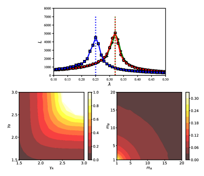
Figure 2: (Top panel) Lifetime of SIS processes on temporal multiplex networks versus $\lambda$ for the uncorrelated (red circles), negative correlated (green triangles) and positively correlated (blue squares) cases. Therein, $\gamma_{\mathbf{x}}=2.1$ and $m_{\mathbf{x}}=1$. The vertical dotted lines with the same colors to the simulations results are the corresponding analytical values obtained from Eq. (7). The simulation results are averaged by $10^{2}$ runs. (Bottom left panel) The analytical thresholds computed by Eq. (7) in the 2-D plane ($\gamma_{A}$,$\gamma_{B}$) when $m_{\mathbf{x}}=1$. (Bottom right panel) The analytical thresholds are calculated from Eq. (7) in the 2-D plane ($m_{A}$,$m_{B}$) when $\gamma_{\mathbf{x}}=1$. In both bottom panels we considered uncorrelated activities.

The first observation is that in all three cases the analytical solutions (vertical dotted lines) agree with the results from simulations. The second observation is that in case of positive correlation between the activities of nodes in two layers, the threshold is significantly smaller than in the other two cases. This is not surprising as the nodes sustaining the spreading in both layers are the same. Thus, effectively, active nodes are capable to infect the double number of other nodes. The thresholds of the uncorrelated and negatively correlated cases are very similar. In fact, due to the heterogeneous nature of the activity distributions, except for few nodes in the tails, the effective difference between the activities matched in reverse or random order is not large, for the majority of nodes. In Figure 2 (bottom panels) we show the behavior of the threshold as function of the activity exponents and the number of links created by active nodes in the two layers. For a given distribution of activity in a layer, increasing the exponent in the other results in an increase of the threshold. This is due to the change of the first and second moments which decrease. In the settings considered here, if both exponents of activity distributions are larger than $2.6$ the critical value of $\lambda$ becomes larger than $1$, as shown in Figure 2 (left bottom). Thus, in such region of parameters, the disease will not spread. For a given number of links created in a layer by each active node, increasing the links created in the other layer results in a quite rapid reduction of the threshold. This is due to the increase of the connectivity and thus the spreading potential of active nodes.

II.3 $M$ layers and $p=1$

In the limit $p=1$, we are able to obtain an expression for the threshold of an SIS process unfolding on $M$ layers. The analytical condition for the spreading of the disease can be written as (see the Appendix for details):

$$\footnotesize\frac{\lambda}{\mu}>\frac{1}{\sum\limits_{y\in\mathbf{x}}\langle a_{y}\rangle_{o}m_{y}+\sqrt{\sum\limits_{y\in\mathbf{x}}\langle a^{2}_{y}\rangle_{o}m^{2}_{y}+\sum\limits_{y=A}^{M-1}\sum\limits_{z>y}^{M}2\langle a_{y}a_{z}\rangle_{o}m_{y}m_{z}}},$$ (8)

where $\mathbf{x}=[A,B,\ldots,Z]$ and $z>y$ implies an alphabetical ordering. The first observation is that in case $h(a_{y},a_{z})=f(a_{y})\delta(a_{z}-a_{y})\;\ \forall y,z\in\mathbf{x}$, thus the activity is the same for each node across each layer, Eq. 8 reduces to:

$$\frac{\lambda}{\mu}>\frac{1}{Mm}\frac{1}{\langle a\rangle+\sqrt{\langle a^{2}\rangle}},$$ (9)

which is the threshold for a single layer activity-driven network in which $m\rightarrow Mm$. This is the generalization of the correspondence between the two thresholds we discussed above for two layers. The second observation is that, in general, increasing the number of layers decreases the epidemic threshold. Indeed, each new layers increases the connectivity potential of each node and thus the fragility of the system to the contagion process. Figure 3 (top panel) shows the analytical behavior of the epidemic threshold up to $M=10$ for the simplest case of uncorrelated (red dots) and positively correlated (blue squares) activities between layers confirming this result. In Figure 3 (bottom panel) we show the comparison between the analytical results and the numerical simulations. The plot shows a perfect match between the two.

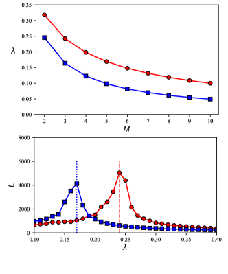
Figure 3: The top panel shows the analytical threshold computed from Eq. (8) versus the number of layers $M$ for the uncorrelated (red circles) and the positively correlated (blue squares) cases. The bottom panel presents the lifetime of SIS processes on temporal multiplex networks when $M=3$ for the uncorrelated (red circles) and the positively correlated (blue squares) cases. The blue dotted line and the red dashed line are the corresponding analytical values. Other parameters are set as $\gamma_{\mathbf{x}}=2.1$, $p=1$ and $m_{\mathbf{x}}=1$.

II.4 Two layers and $0<p<1$

We now turn the attention to the most interesting cases which are different from the two limits of null and total overlap of nodes considered above. For a general value of $p$, we could not find a general closed expression for the epidemic threshold. However, the condition for the spreading can be obtained by investigating, numerically, the spectral properties of the Jacobian (see the Appendix for details). In Figure 4 we show the lifetime of SIS spreading processes unfolding on a multiplex network for three different values of $p$. The top panel shows the uncorrelated case and the dashed vertical lines describe are the analytical predictions. The first observation is that the larger the overlap of nodes between two layers the smaller the threshold. Indeed, by increasing the fraction of nodes active in both layers increases the spreading power of such nodes when they get infected. The second observation is that the analytical predictions match remarkably well the simulations. The bottom panel shows instead the case of positive correlation between the activities of overlapping nodes in the two layers. Also in this case, the larger the overlap the smaller the epidemic threshold. However, the comparison between the two panels clearly show the effects of positive correlations. Indeed, for all the values of $p$ positive correlations push the threshold to smaller values respect to the uncorrelated case. This effect is larger for larger values of overlap. It is important to notice that also here our analytical predictions match remarkably well the numerical simulations.

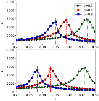
Figure 4: Top panel shows the lifetimes of the SIS processes on the temporal multiplex networks in which the activities of the overlapping nodes in the two layers are uncorrelated for different fraction of overlapping nodes. Bottom panel shows the lifetimes of the SIS processes on the temporal multiplex networks in which the activities of the overlapping nodes in the two layers are positively correlated for different fraction of overlapping nodes. The vertical lines are the corresponding analytical values. Other parameters are set as $\gamma_{\mathbf{x}}=2.1$, $m_{\mathbf{x}}=1$.

In Figure 5 we show the behavior of the (analytical) epidemic threshold as function of $p$ for three types of correlations. The results confirm what discussed above. The larger the overlap the smaller the threshold. Negative and null correlations of overlapping nodes exhibit very similar thresholds. Instead, positive correlations push the critical value to smaller values. Furthermore, the larger the overlap the larger the effect of positive correlations as the difference between the thresholds increases as function of $p$. It is also important to notice how the threshold of a multiplex networks ($p>0$) is always smaller than the threshold of a monoplex ($p=0$) with the same features. Indeed, the presence of overlapping nodes effectively increases the spreading potential of the disease thus reducing the threshold. However, the presence of few overlapping nodes ($p\sim 0$) does not significantly change the threshold, this result and the effect of multiplexity on the spreading power of diseases is in line with what already discussed in the literature for static multiplexes ginestra18-1 ; buono2014epidemics .

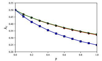
Figure 5: The analytical threshold (Eq. (S18)) is plotted as a function of $p$ for the uncorrelated (red circles), negatively correlated (green triangles) and positively correlated (blue squares) cases. We set $\gamma_{\mathbf{x}}=2.1$ and $m_{\mathbf{x}}=1$.

In Figure 6, we show how the epidemic threshold varies when the average connectivity of the two layers is progressively different and asymmetric. In other words, we investigate what happens when one layer has a much larger average connectivity than the other. This situation simulates individuals engaged in two different social contexts, one characterized by fewer interactions (e.g. close family interactions) and one instead by many more connections (e.g. work environment). In the figure, we consider a multiplex network in which the layer $A$ is characterized by $m_{A}=1$. We then let $m_{B}$ vary from $1$ to $10$ and measure the impact of this variation on the epidemic threshold for different values of $p$. For simplicity, we considered the case of uncorrelated activities in the two layers, but the results qualitatively hold also for the other types of correlations. Few observations are in order. As expected, the case $p=0$ is the upper bound of the epidemic threshold. However, the larger the asymmetry between the two layers, thus the larger the average connectivity in the layer $B$, the smaller the effect of the overlap on the threshold. Indeed, while systems characterized by $m_{B}=1$ and higher overlap feature a significantly smaller threshold respect to the monoplex, for $m_{B}\geq 3$ such differences become progressively negligible and the effects of multiplexity vanish. In this regime, the layer with the largest average connectivity drives the spreading of the disease. The connectivity of layer $B$, effectively determines the dynamics of the contagion, and thus the critical behavior is not influenced by overlapping nodes.

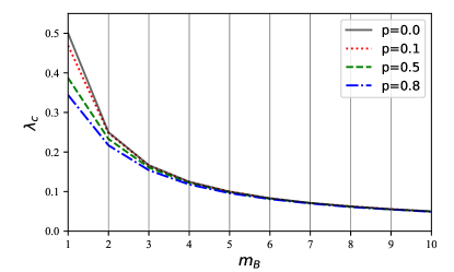
Figure 6: The analytical threshold is plotted as a function of $m_{B}$ when the activities of the overlapping nodes in the two layers are uncorrelated and $m_{A}$ is fixed as 1. We set $\gamma_{\mathbf{x}}=2.1$.

In order to get a deeper understanding on this phenomena, we show the asymptotic number of infected nodes in each layers for $m_{A}=1$ and $m_{B}=10$ in Figure 7. For any $\lambda$ above the threshold the fraction of infected nodes in layer $B$ (bottom panel) is larger than in layer $A$ (top panel ) and is independent on the fraction of overlapping nodes. As discussed above, in these settings the layer $B$ is driving the contagion process and the imbalance between the connectivity patterns is large enough to behave as a monoplex. However, for layer $A$ the contagion process is still highly influenced by $p$. Indeed, as the fraction of overlapping nodes increases layer $A$ is more and more influenced by the contagion process unfolding in $B$. Overall, these results are qualitatively similar with the literature of spreading phenomena in static multilayer networks gomez2013diffusion .

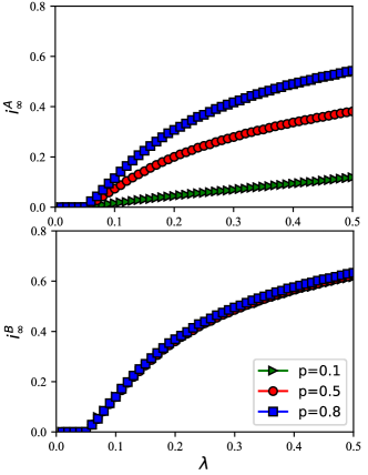
Figure 7: Top panel and bottom panel respectively present the asymptotic fraction of infected nodes in layer $A$ and $B$. The results are averaged by $10^{2}$ simulations. We set $\gamma_{\mathbf{x}}=2.1$ and $m_{\mathbf{x}}=1$.

III Conclusions

We presented a time-varying model of multiplex networks. The intra-layer temporal dynamics follow the activity-driven framework which was developed for single layered networks (i.e. monoplexes). Thus, nodes are endowed with an activity that describes their propensity, per unit time, to initiate social interactions. A fraction $p$ of nodes is considered to be overlapping between layers and their activities are considered, in general, to be different but potentially correlated. In these settings, we studied how multiplexity and temporal connectivity patterns affect dynamical processes unfolding on such systems. To this end, we considered a prototypical model of infectious diseases: the SIS model. We derived analytically the epidemic threshold of the process as function of $p$. In the limit $p=0$ the system is constituted by disconnected networks that behave as monoplexes. In the opposite limit instead ( i.e. $p=1$) the epidemic threshold is function of the first and second moment of the activity distributions as well as by their correlations across layers. We found that, systems characterized by positive correlations are much more fragile to the spreading of the contagion process with respect to negative and null correlations. The threshold also varies as a function of the number of layers $M$. Indeed, with perfect overlapping, each node is present and active in each layer. Thus, the larger $M$ the smaller the epidemic threshold as the spreading potential of each node increases. In the general case $0<p<1$, we could not find a closed expression for the epidemic threshold. However, the critical condition for the spreading can be calculated from the theory by investigating numerically the spectral properties of the Jacobian matrix describing the contagion dynamics. Also in this case, positive correlations of activities across layers help the spreading by lowering the epidemic threshold; while negative and null correlations result in very similar thresholds. Moreover, the larger the overlap between layer the lower the critical condition for the spreading. Indeed, the case of disconnected monoplexes (i.e. $p=0$) is the upper bound for the threshold. Interestingly, the role of the overlap, thus of the multiplexity, is drastically reduced in case the average connectivity in one layer is much larger than the other. In this scenario, which mimics the possible asymmetry in the contact patterns typical of different social contexts (e.g. family VS work environment), one layer drives the contagion dynamics and the critical condition for the spreading is indistinguishable from the monoplex. However, the overlap is still significantly important in the other layer as the fraction of nodes present in both layers largely determines the spreading dynamics.

Some of these results are qualitatively in line with the literature of contagion processes unfolding on static/annealed multiplexes. However, as known in the case of single layered graphs, time-varying dynamics induce large quantitative differences holme11-1 ; holme2015modern . Indeed, the concurrency and order of connections are crucial ingredients for the spreading and neglecting them, in favor of static/annealed representations, generally results in smaller thresholds. While the limits of time-scale separation might be relevant to describe certain types of processes, they might lead to large overestimation of the spreading potential of contagion phenomena.

The model presented here comes with several limitations. In fact, we considered the simplest version of the activity driven framework in which, at each time step, links are created randomly. Future work could explore the role of more realistic connectivity patterns in which nodes activate more likely a subset of (strong) ties and/or nodes are part of communities of tightly linked individuals. Furthermore, we assumed that the activation process is Poissonian and the activity of each node is not a function of time. Future work could explore most realistic dynamics considering bursty activation and ageing processes. All these features of real time-varying networks have been studied at length in the literature of single layered networks but their interplay with multiplexity when dynamical processes are concerned is still unexplored. Thus result presented here are a step towards the understanding of the temporal properties of multiplex networks and their impact on contagion processes unfolding on their fabric.

IV ACKNOWLEDGMENTS

Q.-H Liu would like to acknowledge M. Tang and W. Wang at the Web Science Center for valuable discussions and comments at the beginning of this project. Q.-H Liu acknowledges the support of the program of China Scholarships Council, National Natural Science Foundation of China (Grant No. 61673086) and Science Strength Promotion Programme of UESTC. We thank Alessandro Vespignani and Sandro Meloni for interesting discussions and comments.

V Appendix

V.1 Derivation of the threshold when $M=2$

Integrating over all activity spectrum of Eq. (4), it obtains the following equation,

$$d_{t}I^{\mathbf{x}}=-{\mu}I^{\mathbf{x}}+\lambda m_{\mathbf{x}}\sum\limits_{a}\frac{N_{a}^{\mathbf{x}}-I_{a}^{\mathbf{x}}}{N}a(I^{\mathbf{x}}+I^{o})$$

$$+\lambda m_{\mathbf{x}}\sum\limits_{a}\frac{N_{a}^{\mathbf{x}}-I_{a}^{\mathbf{x}}}{N}\bigg{[}\sum\limits_{a^{\prime}}I_{a^{\prime}}^{\mathbf{x}}a^{\prime}+\sum\limits_{a_{A}^{\prime}}\sum\limits_{a_{B}^{\prime}}I_{a^{\prime}_{A},a^{\prime}_{B}}^{o}a^{\prime}_{\mathbf{x}}\bigg{]}.$$

Initially, $I_{a}^{\mathbf{x}}\approx 0$, $\sum\limits_{a}\frac{N_{a}^{\mathbf{x}}-I_{a}^{\mathbf{x}}}{N}a\approx(1-p)\langle a_{\mathbf{x}}\rangle$. Thus Eq. (V.1) can be further simplified as

$$d_{t}I^{\mathbf{x}}\approx-{\mu}I^{\mathbf{x}}+\lambda m_{\mathbf{x}}(1-p)\langle a_{\mathbf{x}}\rangle(I^{\mathbf{x}}+I^{o})$$

$$+\lambda m_{\mathbf{x}}(1-p)\bigg{[}\sum\limits_{a^{\prime}}I_{a^{\prime}}^{\mathbf{x}}a^{\prime}+\sum\limits_{a_{A}^{\prime}}\sum\limits_{a_{B}^{\prime}}I_{a^{\prime}_{A},a^{\prime}_{B}}^{o}a^{\prime}_{\mathbf{x}}\bigg{]}.$$

Four auxiliary variables defined to simplify Eq. (V.1) are as follows, $\Theta^{A}=\sum\limits_{a}I_{a}^{A}a$, $\Theta^{B}=\sum\limits_{a}I_{a}^{B}a$, $\Theta_{A}^{o}=\sum\limits_{a_{B}}\sum\limits_{a_{A}}I_{a_{A},a_{B}}^{o}a_{A}$ and $\Theta_{B}^{o}=\sum\limits_{a_{A}}\sum\limits_{a_{B}}I_{a_{A},a_{B}}^{o}a_{B}$. Since $\mathbf{x}=[A,B]$, Eq. (V.1) can be expressed as

$$d_{t}I^{A}=-{\mu}I^{A}+\lambda m_{A}(1-p)\langle a_{A}\rangle(I^{A}+I^{o})$$

$$+\lambda m_{A}(1-p)\big{(}\Theta^{A}+\Theta_{A}^{o}\big{)}$$ (S3)

and

$$d_{t}I^{B}=-{\mu}I^{B}+\lambda m_{B}(1-p)\langle a_{B}\rangle(I^{B}+I^{o})$$

$$+\lambda m_{B}(1-p)\big{(}\Theta^{B}+\Theta_{B}^{o}\big{)}.$$ (S4)

Integrating over all activity spectrum of Eq. (5), it obtains the following equation,

$$d_{t}I^{o}=-{\mu}I^{o}+\lambda m_{A}p\langle a_{A}\rangle_{o}(I^{A}+I^{o})$$

$$+\lambda m_{B}p\langle a_{B}\rangle_{o}\big{(}I^{B}+I^{o}\big{)}+p\lambda m_{A}(\Theta^{A}+\Theta_{A}^{o})$$

$$+p\lambda m_{B}(\Theta^{B}+\Theta_{B}^{o}).$$ (S5)

Multiplying both side of Eq. (4) by $a_{\mathbf{x}}$, and integrating over all activity spectrum, we get the following equation

$$d_{t}\Theta^{\mathbf{x}}=-\mu\Theta^{\mathbf{x}}+\lambda m_{\mathbf{x}}(1-p)\langle a_{\mathbf{x}}^{2}\rangle\big{(}I^{A}+I^{o}\big{)}$$

$$+\lambda m_{\mathbf{x}}(1-p)\langle a_{\mathbf{x}}\rangle\big{(}\Theta^{\mathbf{x}}+\Theta_{\mathbf{x}}^{o}\big{)}.$$ (S6)

Replacing $\mathbf{x}$ with A and B in Eq. (V.1) respectively, we have

$$d_{t}\Theta^{A}=-\mu\Theta^{A}+\lambda m_{A}(1-p)\langle a_{A}^{2}\rangle\big{(}I^{A}+I^{o}\big{)}$$

$$+\lambda m_{A}(1-p)\langle a_{A}\rangle\big{(}\Theta^{A}+\Theta_{A}^{o}\big{)}.$$ (S7)

and

$$d_{t}\Theta^{B}=-\mu\Theta^{B}+\lambda m_{B}(1-p)\langle a_{B}^{2}\rangle\big{(}I^{B}+I^{o}\big{)}$$

$$+\lambda m_{B}(1-p)\langle a_{B}\rangle\big{(}\Theta^{B}+\Theta_{B}^{o}\big{)}.$$ (S8)

In the same way, multiplying both sides of Eq. (5) by $a_{\mathbf{x}}$ and integrating over all activity spectrum, it obtains the following two equations

$$d_{t}\Theta_{A}^{o}=-\mu\Theta_{A}^{o}+\lambda m_{A}p\langle a_{A}^{2}\rangle_{o}\big{(}I^{A}+I^{o}\big{)}$$

$$+\lambda m_{B}p\langle a_{A}a_{B}\rangle_{o}\big{(}I^{B}+I^{o}\big{)}+\lambda m_{A}p\langle a_{A}\rangle_{o}\big{(}\Theta^{A}+\Theta_{A}^{o}\big{)}$$

$$+\lambda m_{B}p\langle a_{A}\rangle_{o}\big{(}\Theta^{B}+\Theta_{B}^{o}\big{)}$$ (S9)

and

$$d_{t}\Theta_{B}^{o}=-\mu\Theta_{B}^{o}+\lambda m_{A}p\langle a_{A}a_{B}\rangle_{o}\big{(}I^{A}(t)+I^{o}(t)\big{)}$$

$$+\lambda m_{B}p\langle a_{B}^{2}\rangle_{o}\big{(}I^{B}(t)+I^{o}(t)\big{)}+\lambda m_{A}p\langle a_{B}\rangle_{o}\big{(}\Theta^{A}+\Theta_{A}^{o}\big{)}$$

$$+\lambda m_{B}p\langle a_{B}\rangle_{o}\big{(}\Theta^{B}+\Theta_{B}^{o}\big{)}$$ (S10)

when $\mathbf{x}$ is replaced with A and B, respectively. When the system enters the steady state, we have $d_{t}I^{A}=0$, $d_{t}I^{B}=0$, $d_{t}I^{o}=0$, $d_{t}\Theta^{A}=0$, $d_{t}\Theta^{B}=0$, $d_{t}\Theta_{A}^{o}=0$ and $d_{t}\Theta_{B}^{o}=0$. Set the right hand of Eqs. (V.1)-(V.1) and Eqs. (V.1)-(V.1) as zero, and denote them respectively as F($\Theta^{A}$), F($\Theta^{B}$), F($\Theta_{A}^{o}$), F($\Theta_{B}^{o}$), F($I^{A}$), F($I^{B}$) and F($I^{o}$). Thus, the critical condition is determined by the following Jacobian matrix,

$${J=\left[\begin{array}[]{ccccccc}\frac{\partial F(\Theta^{A})}{\partial\Theta^{A}}&\frac{\partial F(\Theta^{A})}{\partial\Theta^{B}}&\frac{\partial F(\Theta^{A})}{\partial\Theta_{A}^{o}}&\frac{\partial F(\Theta^{A})}{\partial\Theta_{B}^{o}}&\frac{\partial F(\Theta^{A})}{\partial I^{A}}&\frac{\partial F(\Theta^{A})}{\partial I^{B}}&\frac{\partial F(\Theta^{A})}{\partial I^{o}}\\ \frac{\partial F(\Theta^{B})}{\partial\Theta^{A}}&\frac{\partial F(\Theta^{B})}{\partial\Theta^{B}}&\frac{\partial F(\Theta^{B})}{\partial\Theta_{A}^{o}}&\frac{\partial F(\Theta^{B})}{\partial\Theta_{B}^{o}}&\frac{\partial F(\Theta^{B})}{\partial I^{A}}&\frac{\partial F(\Theta^{B})}{\partial I^{B}}&\frac{\partial F(\Theta^{B})}{\partial I^{o}}\\ \frac{\partial F(\Theta_{A}^{o})}{\partial\Theta^{A}}&\frac{\partial F(\Theta_{A}^{o})}{\partial\Theta^{B}}&\frac{\partial F(\Theta_{A}^{o})}{\partial\Theta_{A}^{o}}&\frac{\partial F(\Theta_{A}^{o})}{\partial\Theta_{B}^{o}}&\frac{\partial F(\Theta_{A}^{o})}{\partial I^{A}}&\frac{\partial F(\Theta_{A}^{o})}{\partial I^{B}}&\frac{\partial F(\Theta_{A}^{o})}{\partial I^{o}}\\ \frac{\partial F(\Theta_{B}^{o})}{\partial\Theta^{A}}&\frac{\partial F(\Theta_{B}^{o})}{\partial\Theta^{B}}&\frac{\partial F(\Theta_{B}^{o})}{\partial\Theta_{A}^{o}}&\frac{\partial F(\Theta_{B}^{o})}{\partial\Theta_{B}^{o}}&\frac{\partial F(\Theta_{B}^{o})}{\partial I^{A}}&\frac{\partial F(\Theta_{B}^{o})}{\partial I^{B}}&\frac{\partial F(\Theta_{B}^{o})}{\partial I^{o}}\\ \frac{\partial F(I^{A})}{\partial\Theta^{A}}&\frac{\partial F(I^{A})}{\partial\Theta^{B}}&\frac{\partial F(I^{A})}{\partial\Theta_{A}^{o}}&\frac{\partial F(I^{A})}{\partial\Theta_{B}^{o}}&\frac{\partial F(I^{A})}{\partial I^{A}}&\frac{\partial F(I^{A})}{\partial I^{B}}&\frac{\partial F(I^{A})}{\partial I^{o}}\\ \frac{\partial F(I^{B})}{\partial\Theta^{A}}&\frac{\partial F(I^{B})}{\partial\Theta^{B}}&\frac{\partial F(I^{B})}{\partial\Theta_{A}^{o}}&\frac{\partial F(I^{B})}{\partial\Theta_{B}^{o}}&\frac{\partial F(I^{B})}{\partial I^{A}}&\frac{\partial F(I^{B})}{\partial I^{B}}&\frac{\partial F(I^{B})}{\partial I^{o}}\\ \frac{\partial F(I^{o})}{\partial\Theta^{A}}&\frac{\partial F(I^{o})}{\partial\Theta^{B}}&\frac{\partial F(I^{o})}{\partial\Theta_{A}^{o}}&\frac{\partial F(I^{o})}{\partial\Theta_{B}^{o}}&\frac{\partial F(I^{o})}{\partial I^{A}}&\frac{\partial F(I^{o})}{\partial I^{B}}&\frac{\partial F(I^{o})}{\partial I^{o}}\end{array}\right]}$$ (S18)

If the largest eigenvalue of J is larger than zero, the epidemic will outbreak. Otherwise, the epidemic will die out. Specifically, if $p=0$, two layers are independent and we can get the following two of seven eigenvalues,

$$\Lambda_{A} = -\mu+a_{A}\lambda m_{A}+\lambda m_{A}\sqrt{\langle a_{A}^{2}\rangle}$$

and

$$\Lambda_{B} = -\mu+a_{B}\lambda m_{B}+\lambda m_{B}\sqrt{\langle a_{B}^{2}\rangle},$$

which determine the dynamics on layer A and layer B, respectively. If $p=1$, the largest eigenvalue is

$$\Lambda=-\mu+\lambda\sum\limits_{y\in\mathbf{x}}m_{y}\langle a_{y}\rangle_{o}$$

$$+\lambda\sqrt{2m_{A}m_{B}\langle a_{A}a_{B}\rangle_{o}+\sum\limits_{y\in\mathbf{x}}m_{y}^{2}\langle a_{y}^{2}\rangle_{o}}.$$ (S19)

Further, the critical transmission rate is written as

$$\lambda_{c}=\frac{\mu}{\sum\limits_{y\in\mathbf{x}}m_{y}\langle a_{y}\rangle_{o}+\sqrt{2m_{A}m_{B}\langle a_{A}a_{B}\rangle_{o}+\sum\limits_{y\in\mathbf{x}}m_{y}^{2}\langle a_{y}^{2}\rangle_{o}}}.$$

For $0<p<1$, we could not find a general analytical expression for the eigenvalues of $J$. However, the critical transmission rate can be found by finding the value of $\lambda$ leading the largest eigenvalue of $J$ to zero. In other words, rather the solving explicitly the characteristic polynomial $|J-\Lambda I|=0$ and defining the condition for the spreading $\max{\Lambda}>0$ as done above, we can determined the critical value of $\lambda$ as the value corresponding to the largest eigenvalue to be zero baxter2016unified ; zhuang2017clustering .

V.2 Derivation the threshold for $M$ layers when $p=1$

Assume there are $M$ layers, and let $N_{a_{A},a_{B},...,a_{M}}^{o}$ and $I_{a_{A},a_{B},...,a_{M}}^{o}(t)$ respectively be the number of nodes and the number of infected nodes with activities $(a_{A},a_{B},...,a_{M})$ in layers $(A,B,...,M)$. With the same derivation method of Eq. (5), the evolution equation of $I_{a_{A},a_{B},...,a_{M}}^{o}$ can be written as

$$d_{t}I_{a_{A},...,a_{M}}^{o}=-\mu I_{a_{A},...,a_{M}}^{o}$$

$$+\sum\limits_{i=A}^{M}\lambda m_{i}\big{[}N_{a_{A},...,a_{M}}^{o}-I_{a_{A},...,a_{M}}^{o}\big{]}a_{i}\frac{I^{o}}{N}$$

$$+\frac{N_{a_{A},...,a_{M}}^{o}-I_{a_{A},...,a_{M}}^{o}}{N}\sum\limits_{i=A}^{M}\lambda m_{i}\sum\limits_{a_{A}^{\prime}}\cdots\sum\limits_{a_{M}^{\prime}}I_{a_{A}^{\prime},...,a_{M}^{\prime}}^{o}a_{i}^{\prime},$$

therein, $I^{o}=\sum\limits_{a_{A}^{\prime}}\cdots\sum\limits_{a_{M}^{\prime}}I_{a_{A}^{\prime},...,a_{M}^{\prime}}^{o}$. For the simplicity, let

$$\Theta_{i}^{o}=\sum\limits_{a_{A}^{\prime}}\cdots\sum\limits_{a_{M}^{\prime}}I_{a_{A}^{\prime},...,a_{M}^{\prime}}^{o}a_{i}^{\prime}.$$ (S22)

Multiplying both sides of Eq.(V.2) by $a_{i}$ and integrating over all activity spectrum, it obtains the following equation

$$d_{t}\Theta_{i}^{o}\approx-\mu\Theta_{i}^{o}+\sum\limits_{a_{A}^{\prime}}\cdots\sum\limits_{a_{M}^{\prime}}a_{i}^{\prime}\sum\limits_{j=A}^{M}\lambda m_{j}\frac{N_{a_{A}^{\prime},...,a_{M}^{\prime}}^{o}}{N}a_{j}^{\prime}I^{o}$$ (S23)

$$+\sum\limits_{a_{A}^{\prime}}\cdots\sum\limits_{a_{M}^{\prime}}\frac{N_{a_{A}^{\prime},...,a_{M}^{\prime}}}{N}a_{i}^{\prime}\sum\limits_{j=A}^{M}\lambda m_{j}\Theta_{j}^{o}$$

$$= -\mu\Theta_{i}^{o}+\sum\limits_{j=A}^{M}\lambda m_{j}\langle a_{i}a_{j}\rangle I^{o}+\langle a_{i}\rangle\sum\limits_{j=A}^{M}\lambda m_{j}\Theta_{j}^{o}.$$

Integrating over all activity spectrum of Eq. (V.2), it obtains the following equation

$$d_{t}I^{o}=-\mu I^{o}+\sum\limits_{i=A}^{M}\lambda m_{i}{\langle a_{i}\rangle}I^{o}+\sum\limits_{i=A}^{M}\lambda m_{i}\Theta_{i}^{o}.$$

When the system enters the steady state, $d_{t}I^{o}=0$ and $d_{t}\Theta_{i}^{o}=0$ for $i=A,B,...,M$. Set the right side of Eqs. (S23) and (V.2) as zero, and denote them respectively as $F_{i}(\Theta_{i}^{o})$ and $F(I^{o})$. Thus the critical condition is determined by the following Jacobian matrix

$${J_{M}=\left[\begin{array}[]{cccc}\frac{\partial F_{A}(\Theta_{A}^{o})}{\partial\Theta_{A}^{o}}&\frac{\partial F_{A}(\Theta_{A}^{o})}{\partial\Theta_{B}^{o}}&\cdots&\frac{\partial F_{A}(\Theta_{A}^{o})}{\partial I^{o}}\\ \frac{\partial F_{B}(\Theta_{A}^{o})}{\partial\Theta_{A}^{o}}&\frac{\partial F_{B}(\Theta_{A}^{o})}{\partial\Theta_{B}^{o}}&\cdots&\frac{\partial F_{B}(\Theta_{A}^{o})}{\partial I^{o}}\\ \cdots&\cdots&\cdots&\cdots\\ \frac{\partial F(I^{o})}{\partial\Theta_{A}^{o}}&\frac{\partial F(I^{o})}{\partial\Theta_{B}^{o}}&\cdots&\frac{\partial F(I^{o})}{\partial I^{o}}\end{array}\right].}$$ (S29)

Further, the maximum eigenvalue of matrix $J_{M}$ can be calculated as

$$\Lambda=-\mu+\sum\limits_{i=A}^{M}\lambda\langle a_{i}\rangle m_{i}$$

$$+\sqrt{\sum\limits_{i=A}^{M}\lambda^{2}\langle a_{i}^{2}\rangle m_{i}^{2}+\sum\limits_{i=A}^{M-1}\sum\limits_{j>i}^{M}2\lambda^{2}\langle a_{i}a_{j}\rangle m_{i}m_{j}}$$

Thus, the critical transmission rate is

$$\lambda_{c}=\frac{\mu}{\sum\limits_{i=A}^{M}\langle a_{i}\rangle m_{i}+{\sqrt{\sum\limits_{i=A}^{M}\langle a_{i}^{2}\rangle m_{i}^{2}+\sum\limits_{i=A}^{M-1}\sum\limits_{j>i}^{M}2\langle a_{i}a_{j}\rangle m_{i}m_{j}}}}$$

Further, if the activities of the same node in each layer are the same, the above equation can be simplified as follows,

$$\lambda_{c}=\frac{1}{Mm}\frac{\mu}{\langle a\rangle+{\sqrt{\langle a^{2}\rangle}}}$$ (S32)

References

- (1) Ginestra Bianconi. Multilayer networks. Structure and Function. Oxford University Press, 2018.
- (2) Mikko Kivelä, Alex Arenas, Marc Barthelemy, James P Gleeson, Yamir Moreno, and Mason A Porter. Multilayer networks. Journal of complex networks, 2(3):203–271, 2014.
- (3) Manlio De Domenico, Albert Solé-Ribalta, Emanuele Cozzo, Mikko Kivelä, Yamir Moreno, Mason A Porter, Sergio Gómez, and Alex Arenas. Mathematical formulation of multilayer networks. Physical Review X, 3(4):041022, 2013.
- (4) Stefano Boccaletti, Ginestra Bianconi, Regino Criado, Charo I Del Genio, Jesús Gómez-Gardenes, Miguel Romance, Irene Sendina-Nadal, Zhen Wang, and Massimiliano Zanin. The structure and dynamics of multilayer networks. Physics Reports, 544(1):1–122, 2014.
- (5) Emanuele Cozzo, Guilherme Ferraz de Arruda, Francisco Aparecido Rodrigues, and Yamir Moreno. Multiplex networks basic formalism and structural properties, 2018.
- (6) Stanley Wasserman and Katherine Faust. Social network analysis: Methods and applications, volume 8. Cambridge university press, 1994.
- (7) Lois M Verbrugge. Multiplexity in adult friendships. Social Forces, 57(4):1286–1309, 1979.
- (8) James S. Coleman. Social capital in the creation of human capital. American Journal of Sociology, 94:S95–S120, 1988.
- (9) Michele Starnini, Andrea Baronchelli, and Romualdo Pastor-Satorras. Effects of temporal correlations in social multiplex networks. Scientific Reports, 7(1):8597, 2017.
- (10) Manlio De Domenico, Clara Granell, Mason A Porter, and Alex Arenas. The physics of spreading processes in multilayer networks. Nature Physics, 12(10):901, 2016.
- (11) Mostafa Salehi, Rajesh Sharma, Moreno Marzolla, Matteo Magnani, Payam Siyari, and Danilo Montesi. Spreading processes in multilayer networks. IEEE Transactions on Network Science and Engineering, 2(2):65–83, 2015.
- (12) Sergio Gomez, Albert Diaz-Guilera, Jesus Gomez-Gardenes, Conrad J Perez-Vicente, Yamir Moreno, and Alex Arenas. Diffusion dynamics on multiplex networks. Physical Review Letters, 110(2):028701, 2013.
- (13) Yu-Jhe Huang, Jonq Juang, Yu-Hao Liang, and Hsin-Yu Wang. Global stability for epidemic models on multiplex networks. Journal of mathematical biology, 76(6):1339–1356, 2018.
- (14) Ginestra Bianconi. Epidemic spreading and bond percolation on multilayer networks. Journal of Statistical Mechanics: Theory and Experiment, 2017(3):034001, 2017.
- (15) Saeed Osat, Ali Faqeeh, and Filippo Radicchi. Optimal percolation on multiplex networks. Nature Communications, 8(1):1540, 2017.
- (16) Jian Jiang and Tianshou Zhou. Resource control of epidemic spreading through a multilayer network. Scientific Reports, 8(1):1629, 2018.
- (17) Clara Granell, Sergio Gómez, and Alex Arenas. Dynamical interplay between awareness and epidemic spreading in multiplex networks. Physical Review Letters, 111(12):128701, 2013.
- (18) Emanuele Massaro and Franco Bagnoli. Epidemic spreading and risk perception in multiplex networks: a self-organized percolation method. Physical Review E, 90(5):052817, 2014.
- (19) Dawei Zhao, Lixiang Li, Haipeng Peng, Qun Luo, and Yixian Yang. Multiple routes transmitted epidemics on multiplex networks. Physics Letters A, 378(10):770–776, 2014.
- (20) Camila Buono, Lucila G Alvarez-Zuzek, Pablo A Macri, and Lidia A Braunstein. Epidemics in partially overlapped multiplex networks. PloS one, 9(3):e92200, 2014.
- (21) Dawei Zhao, Lianhai Wang, Shudong Li, Zhen Wang, Lin Wang, and Bo Gao. Immunization of epidemics in multiplex networks. PloS one, 9(11):e112018, 2014.
- (22) Wei Wang, Ming Tang, Hui Yang, Younghae Do, Ying-Cheng Lai, and GyuWon Lee. Asymmetrically interacting spreading dynamics on complex layered networks. Scientific Reports, 4:5097, 2014.
- (23) Yanqing Hu, Shlomo Havlin, and Hernán A Makse. Conditions for viral influence spreading through multiplex correlated social networks. Physical Review X, 4(2):021031, 2014.
- (24) Emanuele Cozzo, Raquel A Banos, Sandro Meloni, and Yamir Moreno. Contact-based social contagion in multiplex networks. Physical Review E, 88(5):050801, 2013.
- (25) Petter Holme and Jari Saramäki. Temporal networks. Physics Reports, 519(3):97–125, 2012.
- (26) Petter Holme. Modern temporal network theory: a colloquium. The European Physical Journal B, 88(9):1–30, 2015.
- (27) N. Perra, B. Gonçalves, R. Pastor-Satorras, and A. Vespignani. Activity driven modeling of time-varying networks. Scientific Reports, 2:469, 2012.
- (28) M. Karsai, N. Perra, and A. Vespignani. Time varying networks and the weakness of strong ties. Scientific Reports, 4:4001, 2014.
- (29) E. Ubaldi, N. Perra, M. Karsai, A. Vezzani, R. Burioni, and A. Vespignani. Asymptotic theory of time-varying social networks with heterogeneous activity and tie allocation. Scientific Reports, 6:35724, 2016.
- (30) Guillaume Laurent, Jari Saramäki, and Márton Karsai. From calls to communities: a model for time-varying social networks. The European Physical Journal B, 88(11):1–10, 2015.
- (31) G. Miritello, E. Moro, and R. Lara. The dynamical strength of social ties in information spreading. Physical Review E, 83:045102, 2010.
- (32) A. Clauset and N. Eagle. Persistence and periodicity in a dynamic proximity network. In DIMACS Workshop on Computational Methods for Dynamic Interaction Networks, pages 1–5, 2007.
- (33) Lorenzo Isella, Juliette Stehlé, Alain Barrat, Ciro Cattuto, Jean-François Pinton, and Wouter Van den Broeck. What’s in a crowd? analysis of face-to-face behavioral networks. Journal of theoretical biology, 271:166, 2011.
- (34) J. Saramäki and E. Moro. From seconds to months: an overview of multi-scale dynamics of mobile telephone calls. The European Physical Journal B, 88(6):1–10, 2015.
- (35) Jari Saramäki, Elizabeth A Leicht, Eduardo López, Sam GB Roberts, Felix Reed-Tsochas, and Robin IM Dunbar. Persistence of social signatures in human communication. Proceedings of the National Academy of Sciences, 111(3):942–947, 2014.
- (36) Vedran Sekara, Arkadiusz Stopczynski, and Sune Lehmann. Fundamental structures of dynamic social networks. Proceedings of the National Academy of Sciences, 113(36):9977–9982, 2016.
- (37) Alain Barrat and Ciro Cattuto. Face-to-face interactions. In Social Phenomena, pages 37–57. Springer International Publishing, 2015.
- (38) N. Perra, A. Baronchelli, D Mocanu, B. Gonçalves, R. Pastor-Satorras, and A. Vespignani. Random walks and search in time varying networks. Physical Review Letter, 109:238701, 2012.
- (39) B Ribeiro, N. Perra, and A. Baronchelli. Quantifying the effect of temporal resolution on time-varying networks. Scientific Reports, 3:3006, 2013.
- (40) Suyu Liu, Nicola Perra, Márton Karsai, and Alessandro Vespignani. Controlling contagion processes in activity driven networks. Physical Review Letters, 112(11):118702, 2014.
- (41) Su-Yu Liu, Andrea Baronchelli, and Nicola Perra. Contagion dynamics in time-varying metapopulation networks. Physical Review E, 87(3):032805, 2013.
- (42) G. Ren and X. Wang. Epidemic spreading in time-varying community networks. Chaos: An Interdisciplinary Journal of Nonlinear Science, 24(2):–, 2014.
- (43) M. Starnini, A. Machens, C. Cattuto, A. Barrat, and R. Pastor-Satorras. Immunization strategies for epidemic processes in time-varying contact networks. Journal of Theoretical Biology, 337:89–100, 2013.
- (44) Michele Starnini, Andrea Baronchelli, Alain Barrat, and Romualdo Pastor-Satorras. Random walks on temporal networks. Physical Review E, 85:056115, May 2012.
- (45) Eugenio Valdano, Luca Ferreri, Chiara Poletto, and Vittoria Colizza. Analytical computation of the epidemic threshold on temporal networks. Physical Review X, 5(2):021005, 2015.
- (46) I. Scholtes, N. Wider, R. Pfitzner, A. Garas, C.J. Tessone, and F. Schweitzer. Causality driven slow-down and speed-up of diffusion in non-markovian temporal networks. Nature Communications, 5:5024, 2014.
- (47) Matthew J Williams and Mirco Musolesi. Spatio-temporal networks: reachability, centrality and robustness. Royal Society Open Science, 3(6):160196, 2016.
- (48) Luis EC Rocha and Naoki Masuda. Random walk centrality for temporal networks. New Journal of Physics, 16(6):063023, 2014.
- (49) Taro Takaguchi, Nobuo Sato, Kazuo Yano, and Naoki Masuda. Importance of individual events in temporal networks. New Journal of Physics, 14(9):093003, 2012.
- (50) Luis EC Rocha and Vincent D Blondel. Bursts of vertex activation and epidemics in evolving networks. PLoS computational biology, 9(3):e1002974, 2013.
- (51) G. Ghoshal and P. Holme. Attractiveness and activity in internet communities. Physica A: Statistical Mechanics and its Applications, 364:603–609, 2006.
- (52) Kaiyuan Sun, Andrea Baronchelli, and Nicola Perra. Contrasting effects of strong ties on sir and sis processes in temporal networks. The European Physical Journal B, 88(12):1–8, 2015.
- (53) Dina Mistry, Qian Zhang, Nicola Perra, and Andrea Baronchelli. Committed activists and the reshaping of status-quo social consensus. Physical Review E, 92(4):042805, 2015.
- (54) R. Pfitzner, I. Scholtes, A. Garas, C.J Tessone, and F. Schweitzer. Betweenness preference: Quantifying correlations in the topological dynamics of temporal networks. Physical Review Letter, 110:19, 2013.
- (55) T. Takaguchi, N. Sato, K. Yano, and N. Masuda. Importance of individual events in temporal networkss. New Journal of Physics, 14:093003, 2012.
- (56) Taro Takaguchi, Naoki Masuda, and Petter Holme. Bursty communication patterns facilitate spreading in a threshold-based epidemic dynamics. PloS one, 8(7):e68629, 2013.
- (57) Petter Holme and Fredrik Liljeros. Birth and death of links control disease spreading in empirical contact networks. Scientific Reports, 4:4999, 2014.
- (58) Petter Holme and Naoki Masuda. The basic reproduction number as a predictor for epidemic outbreaks in temporal networks. PloS one, 10(3):e0120567, 2015.
- (59) Zhen Wang, Chris T Bauch, Samit Bhattacharyya, Alberto d’Onofrio, Piero Manfredi, Matjaž Perc, Nicola Perra, Marcel Salathé, and Dawei Zhao. Statistical physics of vaccination. Physics Reports, 664:1–113, 2016.
- (60) Bruno Gonçalves and Nicola Perra. Social phenomena: From data analysis to models. Springer, 2015.
- (61) E. Ubaldi, A. Vezzani, M. Karsai, N. Perra, and R. Burioni. Burstiness and tie reinforcement in time varying social networks. arXiv preprint arXiv:1607.08910, 2016.
- (62) Laura Alessandretti, Kaiyuan Sun, Andrea Baronchelli, and Nicola Perra. Random walks on activity-driven networks with attractiveness. Physical Review E, 95(5):052318, 2017.
- (63) Matthieu Nadini, Kaiyuan Sun, Enrico Ubaldi, Michele Starnini, Alessandro Rizzo, and Nicola Perra. Epidemic spreading in modular time-varying networks. Scientific Reports, 8(1):2352, 2018.
- (64) M.J. Keeling and P. Rohani. Modeling Infectious Disease in Humans and Animals. Princeton University Press, 2008.
- (65) A. Vespignani. Modeling dynamical processes in complex socio-technical systems. Nature Physics, 8:32–30, 2012.
- (66) Romualdo Pastor-Satorras, Claudio Castellano, Piet Van Mieghem, and Alessandro Vespignani. Epidemic processes in complex networks. Reviews of Modern Physics, 87(3):925, 2015.
- (67) M.V. Tomasello, N. Perra, C.J. Tessone, M. Karsai, and F. Schweitzer. The role of endogenous and exogenous mechanisms in the formation of r&d networks. Scientific Reports, 4:5679, 2014.
- (68) M.E.J. Newman. Networks. An Introduction. Oxford Univesity Press, 2010.
- (69) M. Starnini and R. Pastor-Satorras. Topological properties of a time-integrated activity-driven network. Physical Review E, 87:062807, 2013.
- (70) Federico Battiston, Vincenzo Nicosia, and Vito Latora. Structural measures for multiplex networks. Physical Review E, 89(3):032804, 2014.
- (71) M. Boguña, C Castellano, and R Pastor-Satorras. Nature of the epidemic threshold for the susceptible-infected-susceptible dynamics in networks. Physical Review Letter, 111:068701, 2013.
- (72) M. Morris. Telling tails explain the discrepancy in sexual partner reports. Nature, 365:437, 1993.
- (73) M. Morris and M. Kretzschmar. Concurrent partnerships and transmission dynamics in networks. Social Networks, 17:299, 1995.
- (74) A. Barrat, M. Barthélemy, and A. Vespignani. Dynamical Processes on Complex Networks. Cambridge Univesity Press, 2008.
- (75) Gareth J Baxter, Davide Cellai, Sergey N Dorogovtsev, Alexander V Goltsev, and José FF Mendes. A unified approach to percolation processes on multiplex networks. In Interconnected Networks, pages 101–123. Springer, 2016.
- (76) Yong Zhuang, Alex Arenas, and Osman Yağan. Clustering determines the dynamics of complex contagions in multiplex networks. Physical Review E, 95(1):012312, 2017.