Relativistic charge solitons created due to nonlinear Landau damping: A candidate for explaining coherent radio emission in pulsars

Abstract

A potential resolution for the generation of coherent radio emission in pulsar plasma is the existence of relativistic charge solitons, which are solutions of nonlinear Schrödinger equation (NLSE). In an earlier study, Melikidze et al. (2000) investigated the nature of these charge solitons; however, their analysis ignored the effect of nonlinear Landau damping, which is inherent in the derivation of the NLSE in the pulsar pair plasma. In this paper we include the effect of nonlinear Landau damping and obtain solutions of the NLSE by applying a suitable numerical scheme. We find that for reasonable parameters of the cubic nonlinearity and nonlinear Landau damping, soliton-like intense pulses emerge from an initial disordered state of Langmuir waves and subsequently propagate stably over sufficiently long times, during which they are capable of exciting the coherent curvature radiation in pulsars. We emphasize that this emergence of stable intense solitons from a disordered state does not occur in a purely cubic NLSE; thus, it is caused by the nonlinear Landau damping.

1 INTRODUCTION

Radio pulsars are rotationally powered neutron stars where the radio emission arises well within the neutron star magnetosphere. Observations of pulsar wind nebula suggest that the pulsar wind is composed of a dense electron position pair plasma outflowing from the pulsar. The problem of solving the pulsar magnetosphere equations to obtain estimates of the radiation and pulsar wind from a pulsar, is nontrivial and is a matter of intense research (see, e.g., Spitkovsky 2011; Pétri 2016).

The region around a strongly magnetized ($\mathbf{B}\sim 10^{12}$ G) and fast-spinning neutron star generates enormous electric fields $\mathbf{E}$ and cannot be maintained as vacuum (Goldreich & Julian 1969). Most theories follow the idea that the region around the neutron star is a charge-separated magnetosphere that is force-free, meaning that the electromagnetic energy is significantly larger than all other inertial, pressure, and dissipative forces. To maintain co-rotation in the magnetosphere, the condition $\mathbf{E}\cdot\mathbf{B}=0$ should be satisfied, and this corresponds to a charge number density equal to the Goldreich–Julian density $n_{GJ}=\Omega\,B/(2\pi ce)$, where $\Omega=2\pi/P$, $P$ is the rotational period of the pulsar, $c$ is the velocity of light, and $e$ is the electron charge. The magnetosphere is initially charge-starved, and a supply of charged particles can come from the neutron star or due to pair creation in strong magnetic fields. It was first suggested by Sturrock (1971a) that the region above the polar cap is the most likely place of electron–positron pair generation by magnetic field, and an electromagnetic cascading effect can multiply the pairs to reach density of about $10^{4}-10^{5}n_{GJ}$ (see, e.g., Timokhin & Harding 2015). This value agrees very well with the evidence available from observations of pulsar wind nebula (see, e.g., Blasi & Amato (2011) for a recent review). Thus, pair creation in the polar cap is an essential feature of any pulsar model.

In the last few decades, significant progress has been made in understanding the global force-free magnetosphere physics. In the presence of a copious supply of pair plasma and for the commonly assumed dipolar magnetic field configuration, the steady state global current distribution, the pulsar wind, and the resultant magnetic field structure can be found numerically. A large number of studies has been devoted to finding the global magnetospheric structure (e.g. Contopoulos et al. 1999;Spitkovsky 2006; Timokhin 2006;Kalapotharakos & Contopoulos 2009), and hence the global current distribution is considered to be known. However, most of these global magnetosphere studies do not include the effect of how the plasma is generated in the polar cap. To address this shortcoming, Timokhin & Arons (2013) and Timokhin (2010) revisited two earlier models by Arons & Scharlemann (1979) and Ruderman & Sutherland (1975), where charges can and cannot, respectively, be extracted from the neutron star surface. They combined properties of the global force-free magnetosphere and the local mechanism of pair creation and obtained the solution for the plasma generation in the polar cap numerically. Importantly, Timokhin & Arons (2013) and Timokhin (2010) found that the plasma flow along the open dipolar field lines is non-stationary, as it was suggested by Ruderman & Sutherland (1975).

Radio emission from pulsar is thought to arise from the development of plasma instabilities in the electron–positron plasma streaming relativistically along open dipolar magnetic field lines in the pulsar magnetosphere. However, identifying the physical process that can explain the radio emission properties in pulsars is a challenging problem in astrophysics. The key issues here are:  (i)  to explain the problem of coherency, which manifests itself as observed pulsar radio emission with unrealistically high brightness temperatures $\sim 10^{28}\ldots\;10^{30}$K; and  (ii)  to explain the range of pulsar phenomena, such as micropulses, subpulse drift, nulling/moding, pulsar profile stability, polarization properties, etc.. Generally, the coherent pulsar radio emission can be generated by means of either a maser or a coherent curvature mechanism (e.g., Ginzburg & Zhelezniakov 1975; Ruderman & Sutherland 1975; Melikidze & Pataraya 1980; Melikidze & Pataraya 1984; Kazbegi et al. 1991; Melikidze et al. 2000) emitted in strongly magnetized electron–positron plasma well inside the light cylinder. However, as we will discuss in section 2 (see also Mitra (2017) for a recent review), a large body of observations appear to suggest that the pulsar radio emission is excited via a mechanism of coherent curvature radiation. This radiation emerges from regions of about 500 km above the neutron star surface. The high brightness temperature of this coherent radiation can be explained only if it is excited by charge bunches containing a very large number of charged particles rather than by a single charge. The physics of how these charge bunches are formed and how they emit coherent radio emission is still poorly understood. In this work we will focus on the problem of formation of charge bunches and their stability, and will also address the problem of coherency in pulsar radio emission.

We will rely on a commonly used approximation whereby the non-stationary flow of the plasma along open dipolar field lines is one-dimensional. This approximation is justified because of the strong confinement of the plasma along those lines. We also note that the recent time-dependent model of Timokhin (2010) qualitatively reproduces the non-stationary plasma flow that was proposed in the classical radio pulsar emission model of Ruderman & Sutherland (1975, hereafter RS75). While the RS75 model does not solve for the detailed time-dependent effect of pair creation, it does give a prescription of how to estimate the plasma parameters in the radio emission region. Since we are primarily interested in simple estimates of the plasma parameters, we will use the RS75 model as the starting point of our study.

RS75 were amongst the first to propose a model that attempted to explain the overall aspect of the pulsar emission, i.e., both coherency and radio pulsar observational phenomenology. In their model, there exists an inner acceleration region close to the polar cap, where a relativistic non-stationary flow of the electron–positron pair plasma can be established. To address the problem of coherent radio emission, RS75 suggested that charge bunches could be formed due to development of a two-stream instability that results from the overlap between fast-moving and slow-moving particles of the non-stationary plasma. This instability leads to the formation of linear electrostatic Langmuir waves, whose frequency is the plasma frequency. As the Langmuir wave propagates along the magnetic field, each type of particles is subject to the sinusoidal electric field, where for half of its period the field bunches together charges of one sign, while for the next half-period it bunches together charges of the opposite sign. RS75 proposed that these charge bunches can excite the coherent radio emission.

However, the explanation of coherent emission as occurring from such charge bunches has the following fundamental difficulty, as was pointed out by Lominadze et al. (1986) and Melikidze et al. (2000) (hereafter MGP00). On one hand, the spatial dimension $\Lambda_{b}$ of an emitting bunch (along the magnetic field lines) should be smaller than the period of the coherently emitted wave $\lambda_{c}$:

$$\lambda_{c}>\Lambda_{b}.$$ (1a)

Indeed, if $$\lambda_{c}<\Lambda_{b} \lambda_{l} \Lambda_{b}\approx\lambda_{l}/2 \omega=2\pi c/\lambda$$, then different regions of the bunch would emit independently and hence incoherently. As described above, the bunching is caused by linear Langmuir waves (having wavelength ), and the size of a bunch is about half of the wave’s period; i.e., . Since Langmuir waves have an approximately vacuum dispersion relation, , the condition (1a) that the emission be coherent amounts to

$$\omega_{c}<2\omega_{l},$$ (1b)

where $\omega_{c}$ and $\omega_{l}$ the characteristic frequency of the emitted waves and the Langmuir waves, respectively. On the other hand, the temporal period of the emitted wave, i.e. $\mathcal{T}_{c}=2\pi/\omega_{c}$, cannot exceed the time window over which the emitting bunch exists; this time window is half of the period of the Langmuir wave, i.e. $\mathcal{T}_{b}=\pi/\omega_{l}$. Indeed, if the condition

$$\mathcal{T}_{c}<\mathcal{T}_{b}$$ (2a)

does not hold, the charge bunch would disperse away before it has the chance to emit a radio wave. Equivalently to (2a), one must have

$$\omega_{c}>2\omega_{l}\,.$$ (2b)

Clearly, the above two conditions: (1b) (coherency of the emission) and (2b) (non-dispersal of the charge bunch) are in contradiction with each other.

In the last few decades, significant refinement of the basic physical ideas that were postulated by RS75 has been achieved both theoretically and observationally (e.g., MGP00; Gil et al. 2004; Mitra et al. 2009; Melikidze et al. 2014). To circumvent the fundamental difficulty described in the previous paragraph, MGP00 accounted for nonlinear effects due to sufficiently strong two-stream instability in the relativistic plasma. Their theory led to the nonlinear Schrödinger equation (NLSE) with a nonlinear Landau damping term, which describes propagation of the slowly varying envelope of Langmuir waves. It is important to clarify that the same mechanism — the interaction between packets of Langmuir waves and charged particles in the plasma — leads to the appearance of both the local and nonlocal nonlinear terms in the NLSE (see section 4 for details). Therefore, strictly speaking, both these terms are to be kept in a comprehensive analysis of the problem. However, no analytical solution of the NLSE with the nonlocal nonlinear Landau damping term is known. Thus, by way of approximation, MGP00 neglected the nonlinear Landau damping term, assuming it to be small, and showed that for reasonable pulsar parameters, the solution of the NLSE leads to formation of a nonlinear solitary wave, i.e., a soliton, which carries an effective charge. Unlike the “half-period" charge bunches in the linear RS75 theory, the charge solitons can exist for times much longer than $\pi/\omega_{l}$. Thus, since $\mathcal{T}_{b}$ is no longer related to $\pi/\omega_{l}$, condition (2b) can no longer be deduced from condition (2a). (Let us note, in passing, that for solitons, condition (1b) also does not follow from condition (1a), because the soliton’s length is much greater than the spatial period of the carrier Langmuir wave.) Hence, the bunch non-dispersal condition (1b) no longer contradicts the coherency condition (1a), and therefore charge solitons, at least in principle, can excite coherent radio emission in the plasma.

Yet, an explanation of the coherent emission relying on solitons of the “pure" NLSE without a nonlinear Landau damping term has a shortcoming of its own. A stably propagating soliton (or a few solitons) is known to emerge only from a certain class of initial conditions — a localized one. However, there is no reason to assume that such an initial state actually occurs in a magnetospheric plasma; rather, the initial condition there is likely to be a nonlocalized Langmuir wave with a randomly modulated envelope. A solution developing from such an initial condition is known to be a disordered ensemble of solitons and a non-solitonic part of the solution (so-called linear dispersive waves). In this disordered state, solitons continuously appear and disappear as a result of their interaction with one another and with linear dispersive waves; see, e.g., Solli et al. (2007); Fedele et al. (2010); Lakoba (2015); Agafontsev & Zakharov (2015); Gelash & Agafontsev (2018). Consequently, such “flickering" solitons do not exist for times long enough that would let conditions (2a) and (1a) hold simultaneously. Thus, a mechanism that would preserve a soliton’s individuality for a sufficiently long time, is required for the MGP00 theory to become a strong contender in explaining the pulsar coherent radio emission.

In this paper we demonstrate that taking into account the effect of nonlinear Landau damping in the MGP00 theory provides such a soliton-stabilizing mechanism. The main part of this paper is organized as follows. In section 2 we briefly describe the observational evidence from radio pulsars that motivates invoking the charge soliton model. In section 3 we briefly outline the generation mechanism and features of the radio emitting plasma based on the polar-cap RS75 class of models. In section 4 we introduce the concept of the NLSE in pulsar plasma, and in section  5 we discuss the range of parameters which are reasonable to expect in charge bunches of plasma near a pulsar. In section 6 we present the main results: a numerical observation of an intense long-living electrostatic pulse with an internal structure, which is formed in the NLSE model due to the nonlinear Landau damping. In section 7 we summarize the results. Appendix A contains a description of the numerical method, Appendix B discusses the appropriateness of using periodic boundary conditions in the numerical simulations, and Appendix C lists definitions of notations used in this work.

2 OBSERVATIONAL EVIDENCE OF COHERENT CURVATURE RADIATION OF PULSARS

Radio pulsar phenomenological studies performed over the years provide a sound basis for understanding some general properties of the pulsar radio emission (see, e.g., Mitra 2017). Pulsars emit periodic signals with period ranging from about 1 msec to 8.5 sec, and the pulsed emission is restricted to an emission window which is typically 10% of the pulse period. In this study we will focus on properties of so-called normal pulsars, whose periods, $P$, are longer than $\sim$50 msec and whose surface dipolar magnetic field is about $\sim 10^{12}$ G. In normal pulsars the average pulse profile, which is obtained by averaging a large number of single pulses, is seen to be highly structured and can consists of one to several Gaussian-like components.

Pulsars are also highly linearly polarized, and the polarization position angle (PPA) across the pulsar profile shows a characteristic S-shaped swing. This has been interpreted by the rotating vector model (Radhakrishnan & Cooke 1969) as a signature of emission arising due to curvature radiation from charge bunches moving along the open dipolar magnetic field lines. The steepest gradient (SG) point of the PPA traverse corresponds to the fiducial magnetic plane which contains the rotation and magnetic axes.

Pulsar profile along with linear polarization information is used in a statistical sense to infer that the pulsar radio emission beam is composed of a central core emission surrounded by nested conal emission. The components in the single pulses are more dynamic in their location inside the pulse window, which leads to such phenomena as:  (i)  subpulse drifting, where in subsequent single pulses the emission components are seen to systematically move across the pulse window;  (ii)  the small-scale quasiperiodic temporal structures seen in components of single pulses called "micro-structures"; and  (iii)  nulling and moding, where the average or radio emission either switches off completely or changes its pattern for a certain duration, and then returns back to its original state. All these phenomena can be considered as non-stationary effects in the pulsar magnetospheric plasma.

In the following three subsections we will briefly summarize the basic outcome from pulsar radio observations and point out the constraints they provide in formulation of the theory of coherent radio emission from pulsar.

2.1 Emission height

There are three different techniques that can be used to determine the location where the radio emission detaches from the pulsar magnetosphere. Two of these techniques, namely the geometrical method and the aberration and retardation (A/R) method, rely on the fact that pulsar emission arises in the region of open dipolar diverging magnetic field lines; merits, drawbacks, and usage of these height estimation methods can be found in Mitra & Li (2004) and Dyks (2008). Between these two methods, the A/R method, proposed by Blaskiewicz et al. (1991), is known to give more robust estimates for radio emission locations in normal pulsars. Moreover, the A/R method revealed that emission heights can be estimated independently of pulsar’s geometry (see Dyks et al. 2004). The A/R effect is seen as a shift between the center of the total intensity profile and the fiducial plane containing the magnetic and spin axes, which is often identified as the steepest gradient point of the PPA traverse or the peak of the core emission. The A/R methods suggest that the core and conal emission, i.e. the overall emission across the pulsar beam, arises from approximately the same height (Mitra et al. 2016). A few notable studies dedicated to finding emission heights using the A/R method are: Blaskiewicz et al. (1991), von Hoensbroech & Xilouris (1997), Mitra & Li (2004), Mitra & Rankin (2011), Weltevrede & Johnston (2008). These studies suggest that the radio emission arises from about $\sim$500 km above the neutron star’s surface (see also Fig. 3 of Mitra 2017) The third method for finding emission heights is based on using pulsar scintillation. In this method, one uses the fact that the emission from the compact emission region of the pulsar passes through the interstellar medium which can act as a varying lens, thus modulating the pulsar signal. The nature of this modulation depends on the spatial transverse extent of the source, which can be recovered by performing extremely high spatial resolution interferometry. The method has been applied successfully on a few pulsars, and accurate results are only available for the Vela pulsar which imply that the spatial transverse extent of the emission source is about 4 km and the corresponding radio emission altitude is estimated to be about 340 km, in agreement with the other methods (Johnson et al. 2012).

The pulsar radio emission height $R_{em}\sim 500$ km is a very significant input to the pulsar radio emission mechanism problem. The only plasma instability that can develop at these heights (where the magnetic field is very strong and the plasma is constrained to move along the magnetic field lines) is the two–stream instability. Hence, resonance-type instabilities like the cyclotron maser instability (which can develop only near the light cylinder, where the magnetic field is weak), can be ruled out.

2.2 Evidence for curvature radiation

The estimated emission heights $R_{em}$ is the location where the emission detaches from the pulsar magnetosphere. It is quite possible that the pulsar emission is generated in the emitting plasma at a certain height $R_{g}<R_{em}$, and then emerges out of the plasma at $R_{em}$. There is, however, no direct way to probe this effect, and one has to resort to wave propagation properties in electron–positron plasma at such strong magnetic fields. Once the radiation is generated in the plasma, it naturally splits as ordinary, or O-mode (polarized in the plane of the wave vector $\mathbf{k}$ and the magnetic field $\mathbf{B}$) and the extraordinary, X-mode (polarized perpendicularly to the $\mathbf{k}$ and $\mathbf{B}$ plane). The O-mode strongly interacts with the plasma and is ducted along the magnetic field lines or can be damped, while the X-mode can escape the plasma at $R_{g}\sim R_{em}$ as if it were in vacuum (see Gil et al. 2004, Mitra et al. 2009, and Melikidze et al. 2014 for details).

It turns out that there is multiple observational evidence that allows determination of the orientation of the emerging polarization direction with respect to the dipolar magnetic field planes. The most direct evidence comes from the x-ray image of the Vela pulsar wind nebula and fiducial or the SG point of the absolute PPA, which can be used to establish that the electric vector emanating out of the pulsar is orthogonal to the magnetic field planes, and hence represents the extraordinary (X) mode. Lai et al. (2001) also showed that the proper motion direction (PM) of the pulsar is aligned with the rotation axis. Johnston et al. (2005) and Rankin (2007) produced a distribution of the quantity $|{\rm PM}-\mbox{absolute PPA}|$ for a few pulsars and found a bimodal distribution around zero and 90^∘. Assuming that the pulsar’s PMs are parallel to the rotation axis, the bimodality could be explained as occurring due to the emerging radiation being either parallel or perpendicular to the magnetic field planes, since pulsars are known to have orthogonal polarization modes. Alternatively, PMs of pulsars can also be parallel or perpendicular to the rotation axis. While both the above explanations are possible, it is clear that the electric vectors of the waves which detach from the pulsar magnetosphere to reach the observer follow the magnetic field planes.

These observations can hence be interpreted as suggesting that the observed emission is associated with curvature radiation mechanism, since this is the only known emission mechanism that can distinguish the magnetic field planes. Further evidence of curvature radiation can also be obtained from single pulse polarization, where Mitra et al. (2009) demonstrated that the instantaneous polarization of components of single pulses closely follow the average PPA.

2.3 Evidence for non-dipolar surface magnetic field

At a distance of $R_{em}$ where the pulsar radio emission originates, the magnetic field is significantly dipolar. However, the magnetic field at the surface of the neutron star needs to be significantly non-dipolar, so that a sufficient amount of the electron–positron pair plasma can be generated to explain the observed pulsar radiation. Pulsars are known to slow down at a certain rate $\dot{P}$, and this slow-down can be used to estimate only the surface dipolar magnetic field component to be $B_{d}\sim 6\times 10^{19}\sqrt{P\dot{P}}$ G; here $P$ is the pulsar rotation period (in seconds) and $\dot{P}$ is non-dimensional. There is, however, observational evidence that suggests the presence of a surface non-dipolar magnetic field. The strongest piece of such evidence, from which the existence of non-dipolar magnetic field can be inferred, comes from the discovery of a long-period ($P=8.5$ sec) pulsar PSR J2144$-$3933 (Young et al. 1999). Gil & Mitra (2001) argued that significant creation of pair plasma in this pulsar, which is essential for producing the radio emission, can only happen if the radius of curvature of the surface magnetic field is $\rho\sim 10^{5}$ cm, which is about an order of magnitude smaller than $\rho$ values in normal pulsars with $P\sim 1$. The smaller value of $\rho_{c}$ in PSR J2144$-$3933 implies that the magnitude of the surface non-dipolar magnetic field there is about 10¹⁴ G, which is about 100 times higher than the dipolar magnetic field. Furthermore, in some radio pulsars, soft x-ray blackbody radiation is seen from hot polar caps, and the estimated area of the polar cap is often found to be smaller than the dipolar area, suggesting the presence of a strong non-dipolar field on the neutron star surface (see, e.g., Table 1 of Geppert (2017) and references therein).

Thus, in summary, the basic input to the pulsar emission models from observations is that coherent radio emission is excited in a non-stationary plasma flowing away from a pulsar and detaches from it at a height of about a few hundred km above the pulsar’s surface, in a region of open dipolar magnetic field lines. The magnetic field on the neutron star surface, however, is significantly non-dipolar.

3 Plasma condition in the magnetosphere and Mechanism for Radio Emission in Pulsars

As we have described in the Introduction, the RS75 class of the polar cap models provide a framework whereby the observed coherent curvature radiation is attributed to the emission of radio waves by charge bunches in the plasma. In this section we will summarize subsequent stages of creation of this radio emission. We will refer to a pulsar, i.e., a neutron star, having the following parameters: radius $R_{s}$, pulsar period $P$ (measured in seconds), pulsar slow-down rate $\dot{P}$, surface magnetic field $B_{s}$, and dipolar magnetic field $B_{d}$ (see the beginning of section 2.3). For future use we also introduce the ratio $b=B_{s}/B_{d}$, a non-dimensional parameter $\dot{P}_{-15}=\dot{P}/(10^{-15})$, which is assumed to be of order one, and the vector of angular velocity of the rotating star, whose magnitude is $\Omega=2\pi/P$.

3.1 Gap formation

RS75 suggested that if the condition $\mathbf{\Omega\cdot B_{s}}<0$ holds above the pulsar polar cap, then the polar cap is positively charged. They envisaged a situation where initially there is only a limited supply of stray positive charges above the polar cap, which is relativistically flowing away from the pulsar along open magnetic field lines as a pulsar wind. Consequently, if the binding energy of the ions in the neutron star surface is sufficiently strong, then the region above the polar cap will be deficient in positive charges, and a vacuum gap can be created, where an enormously high electric field exists. Photons of energy $>2m_{e}c^{2}$, where $m_{e}$ is the mass of electron, are split inside the vacuum gap into electron–positron pairs, and the electric field in the gap separates these two types of charges. They are then further accelerated along the curved magnetic field lines (hence the term ‘curvature radiation’) and can generate high-energy curvature photons, which, in their turn, after traveling some mean free path, can produce other electron–positron pairs. In terms of pulsar parameters, the potential drop $\Delta V$ across the gap and the gap’s height $h$ can be expressed as

$$\Delta V\sim 2\times 10^{12}b^{-1/7}P^{-3/14}\dot{P}_{-15}^{-1/14}\rho_{6}^{4/7}~{}~{}\rm{V},$$ (3)

$$h\sim 5\times 10^{3}b^{-4/7}P^{1/7}\dot{P}_{-15}^{-2/7}\rho_{6}^{2/7}~{}~{}\rm{cm}\,\gtrsim 10^{4}~{}\mathrm{cm}\,.$$ (4)

Here $\rho_{6}\equiv\rho\,({\rm cm})\,\times\,10^{-6}$, where $\rho$ is the curvature radius of magnetic field lines in the gap region. To obtain the numeric estimate in (4), we used the values $\rho_{6}\sim P\sim\dot{P}_{-15}\sim 1$ and $b\sim 10$.

3.2 Spark formation

A number of such localized discharges can be formed in the gap, and each such a discharge causes a pair creation cascade. The electric field in the gap accelerates the electrons towards the stellar surface, while the positrons are accelerated away from the surface. At the top of the gap these positrons acquire Lorentz factors of $\gamma_{b}$ such that

$$\gamma_{b}\approx e\Delta V/m_{e}c^{2}\,\sim\,2\times 10^{6}.$$ (5)

As these particles move away from the gap to the region where $\mathbf{E\cdot B}=0$, they continue to create high energy photons, which further create pairs, and this cascade leads to the generation of a cloud of secondary electron–positron plasma, which has a significantly lower Lorentz factor with a mean value of $\gamma_{p}$. If the positron number density in the primary beam is $n_{b}$, then the number density of pairs in the secondary plasma can be estimated as $n_{p}\sim(0.5\gamma_{b}/\gamma_{p})n_{b}$, and thus the density of the secondary plasma increases by a factor $\kappa=n_{p}/n_{b}$. In this work we will use the value $\kappa\sim 10^{4}$ (Sturrock 1971b). The burst of pair production process increases the charge density along the gap discharge stream and screens the potential in the gap. This process develops exponentially, and after a certain distance from the star, which is estimated to be $\sim 30-40h\sim 500~{}{\rm m}$ (RS75), the charge density becomes close to $n_{GJ}$, and the particle acceleration process stops. During this time the discharge spreads in the lateral direction thus acquiring a width of $\sim h$. We will call this fully formed discharge a spark, and each spark is associated with a secondary plasma cloud. According to the above description, such a cloud has the shape of a column with a longitudinal dimension of $\sim 500~{}{\rm m}$ and a diameter of $\gtrsim 10~{}{\rm m}$ near the pulsar’s surface. As the cloud moves away from the star to a distance $R$ from its center, the cloud’s diameter grows proportionally to $(R/R_{s})^{1.5}$ due to the divergence of dipolar magnetic field lines.

The charge number density of the primary beam, $n_{b}=n_{GJ}$, can be expressed in terms of pulsar parameters as

$$n_{GJ}\sim 6\times 10^{5}\left(\dot{P}_{-15}/P\right)^{0.5}R^{-3}_{50}\rm{cm^{-3}},$$ (6)

where $R_{50}=R/(50R_{s})$; and a value of $R_{s}=10$ km will be used for subsequent calculations in this paper. Here and below we normalize the distance to $50R_{s}$ since the coherent radio emission occurs around that altitude (see next subsection); hence $R_{50}\sim 1$. The number density of the secondary plasma is $n_{p}=\kappa n_{GJ}$, and hence the mean Lorentz factor of the secondary plasma can be estimated to be

$$\gamma_{p}\approx\gamma_{b}/(2\kappa)\sim 100\,.$$ (7)

The plasma frequency $\omega_{p}$ is given by

$$\omega_{p}\sim 4\times 10^{9}R_{50}^{-1.5}\kappa_{4}^{0.5}(\dot{P}_{-15}/P)^{0.25}~{}\rm{s}^{-1},$$ (8)

where $\kappa_{4}=\kappa/10^{4}\,\sim\,1$.

For later use in the next subsection, we will also mention that once the spark-associated plasma cloud leaves the polar cap and the gap’s potential can no longer be screened, the next discharge can be initiated. Thus, the distance between two consecutive plasma clouds is estimated to be $\sim h$.

3.3 Development of linear two-stream instability in secondary plasma

The overall sparking process leads to a non-stationary flow of successive plasma clouds flowing along a bundle of magnetic dipolar field lines. Indeed, since the magnetic field is strong and the ratio of the plasma frequency to cyclotron frequency $\omega_{p}/\omega_{B}\ll 1$ at the radio emission heights, the charges are confined to move tightly along the magnetic field lines. Therefore, we will hence restrict ourselves to discussing the plasma properties in a one-dimensional flow.

It should be mentioned that within each plasma cloud, distribution functions of electrons and positrons differ from each other (see the discussion around Eq. (11) below). RS75 pointed out that it could be a reason for the two-stream instability. On the other hand, Usov 1987 suggested that due to an overlap of the slow- and fast- moving particles of two successive clouds, a two-stream instability can develop. Asseo & Melikidze (1998) showed that this two-stream instability provides a sufficiently strong Langmuir turbulence in the plasma, with the frequency of Langmuir waves $\omega_{l}$ being

$$\omega_{l}\approx\gamma_{p}\omega_{p}\sim 4\times 10^{11}R_{50}^{-1.5}\,.$$ (9)

Moreover, disturbances of the envelope of these slowly modulated Langmuir waves, obeying the NLSE (MGP00), propagate with the group velocity that can coincide with the velocity of some portion of the charged particles. This occurs because of the aforementioned spread of particle velocities, both within one species and well as between the two species. This synchronism is behind the mechanism of the nonlinear Landau damping, first derived for this situation by MGP00. To quantify that effect, as well as the magnitude of nonlinear and dispersive terms in the NLSE in the next section, we will need to refer to the velocity distribution functions of electrons and positrons in the secondary plasma. They can be approximated by a Gaussian function centered around momentum $p_{\alpha}$ and having a spread of $p_{T}$:

$$f_{\alpha}\propto\exp[-((p-p_{\alpha})/p_{T})^{2}]\sim\exp[-((\gamma-\gamma_{s,\,\alpha})/\gamma_{T})^{2}].$$ (10)

Here $\alpha=+$ or $-$, corresponding to positron or electron species of the plasma, and $\gamma_{s,\,\alpha}$ and $\gamma_{T}$ are the Lorentz factors corresponding to the momenta $p_{\alpha}$ and $p_{T}$. It is important to notice that due to the flow of plasma along the curved magnetic field lines, the distribution functions of positrons and electrons become unequal: $f_{+}\neq f_{-}$ (Cheng & Ruderman 1979). It was further shown by Asseo & Melikidze (1998) that

$$|\gamma_{s,\,+}-\gamma_{s,\,-}|/\gamma_{p}\equiv\Delta\gamma/\gamma_{p}\approx\Delta\sigma\gamma_{p}^{3}/\gamma_{b}\,,$$ (11)

where the value of parameter $\Delta\sigma$ depends on whether the surface magnetic field at polar cap region is assumed to be strictly dipolar or to have a multipolar structure (MGP00); see section 2.3. Importantly for the estimate of the nonlinear Landau damping parameter is section 5 below, it was shown in MGP00 that $\Delta\gamma/\gamma_{p}$ is in the range $0.5\ldots 2$.

Finally, an important parameter when solving the NLSE in subsequent sections is the distance from the pulsar’s surface where the two-stream instability develops, thereby leading to strong Langmuir turbulence and hence strong radio emission. Simple kinematic estimates performed by MGP00 show that the distance at which this instability can set in is $\sim 2\gamma_{p}^{2}h\gtrsim 200$ km. In terms of pulsar parameters, this can be written as

$$R_{\rm onset}\sim 20R_{s}\times\gamma_{2}^{2}\rho_{6}^{2/7}b^{-4/7}B_{12}^{-4/7}P^{3/7}\,,$$ (12a)

where $$B_{12}=B_{d}/10^{12}~{}~{}{\rm{G}} \gamma_{2}=\gamma_{p}/10^{2} (R/R_{s})^{1.5}$$ and . The longitudinal dimension of the instability region is limited by the divergence of the magnetic field lines, which leads to a decrease of the plasma charge density in proportion to . As suggested in Asseo & Melikidze (1998), the dimension of this region is

$$\Delta R\sim 500~{}~{}{\rm km}.$$ (12b)

Therefore, we can estimate that most of the radiation comes from the middle (or the second half) of this region, where, on one hand, the Langmuir turbulence is already strong because the two-stream instability has had sufficient time to develop, and, on the other hand, is still strong enough, having not been weakened by the divergence of the magnetic field lines. Thus, the location of the radiating region can be estimated to be

$$R_{em}\sim(R_{\rm onset}+\Delta R/2)\sim 500~{}~{}{\rm km}$$ (12c)

from the star. Equivalently, one has $R_{50}\sim 1$ in this region. This is the value we used in (8) to obtain the estimate (9). Let us note that estimate (12c) is in good agreement with observations, as discussed in section 2.1.

In the next two sections we will discuss the nonlinear equation satisfied by the envelope of the Langmuir waves and the range of parameters for which it should be solved. Then, in section 6, we will demonstrate that the solution of that equation is capable of explaining features of the observed coherent radiation from pulsars.

4 Nonlinear dynamics and creation of relativistic charge solitons

The nonlinear interaction of an electric field with plasma, which involves the nonlinear Landau damping as an integral part, has been studied for a long time. In one of the early studies, Ichikawa & Tanuiti (1973) derived the NLSE with the nonlinear Landau damping term for the non-relativistic electron–ion plasma. This equation has the form:

$$i\frac{\partial E_{\|}}{\partial\tau}+G\frac{\partial^{2}E_{\|}}{\partial\chi^{2}}+qE_{\|}\left(\big{|}E_{\|}\big{|}^{2}+\frac{s}{\pi q}\;-\int\frac{|E_{\|}(\chi^{\prime},\tau)|^{2}\;d\chi^{\prime}}{\chi-\chi^{\prime}}\;\right)\,=\,0.$$ (13)

where $E_{\|}$ is the amplitude of the electric field and $\tau$ and $\chi$ are the space and time coordinates. More details about these variables and the coefficients in (13) will be given when we discuss its application to the pulsar plasma. Nonlinear Landau damping is

Later on, Pataraia & Melikidze (1980) and Melikidze & Pataraya (1980) showed that the evolution of the envelope of Langmuir wave packets is also governed by the NLSE (13) for the relativistic electron–ion and electron–positron plasmas, respectively. Here, as well as for other types of plasmas, the interaction between the charged particles of the plasma and those packets of Langmuir waves whose group velocity coincides with the velocity of the particles, leads both to the purely cubic, local term in the NLSE and the nonlocal, nonlinear Landau damping term. Let us also note that the NLSE of the same form (13) has been derived for other types of plasmas; see, e.g., Ehsan et al. (2009); Chatterjee & Misra (2015); Misra et al. (2017); Chaudhuri & Roy Chowdhury (2018); to name just a few studies. Related plasma models that also account for nonlinear Landau damping can be found, e.g., in Meiss & Morrison (1983); Roy Chowdhury et al. (1988); Flå et al. (1989); Misra & Barman (2015); Barman & Misra (2017).

MGP00 applied the NLSE (13) to the pulsar plasma. In that context, $E_{\|}$ in (13) is the amplitude of the electric field which is parallel to the external magnetic field and $\chi$ and $\tau$ are the dimensional space and time coordinates in the moving frame of reference (MFR). They are related to the coordinates $\chi_{\circ}$ and $\tau_{\circ}$ in the observer frame of reference (OFR) by:  $\chi=\gamma_{\circ}(\chi_{\circ}-v_{g}\tau_{\circ})$ and $\tau=\gamma_{\circ}(\tau_{\circ}-(v_{g}/c^{2})\chi_{\circ})$, where $v_{g}$ is the group velocity of Langmuir waves and $\gamma_{\circ}\approx\gamma_{p}$ is the corresponding Lorentz factor. In particular, any length and time intervals in the OFR are related to such intervals in the MFR by:  $\delta\chi_{\circ}=\delta\chi/\gamma_{p}$ and $\delta\tau_{\circ}=\delta\tau/\gamma_{p}$. The coefficients $G$, $q$ and $s$ in Eq. (13) correspond to the dispersion, cubic nonlinearity, and nonlinear Landau damping terms, respectively. These coefficients depend on the distribution functions $f_{\alpha}(p)$ (see section 3.3) and other parameters of the plasma and are given by Eq. (A20) in MGP00:

$$G = \frac{1}{4}\frac{\gamma_{p}^{2}c^{2}}{\omega_{p}}G_{d}\,,$$ (14)

$$q = \left(\frac{e^{2}}{m_{e}c}\right)^{2}\frac{1}{\gamma_{p}^{2}\omega_{p}}q_{d}\,,$$ (15)

$$s = \left(\frac{e^{2}}{m_{e}c}\right)^{2}\frac{1}{\gamma_{p}^{2}\omega_{p}}s_{d}\,,$$ (16)

where $G_{d}$, $q_{d}$ and $s_{d}$ depend only on the distribution functions of the plasma. Typical plots of the coefficient $G_{d}$ and the ratio $s_{d}/q_{d}$ as functions of the thermal spread $\gamma_{T}/\gamma_{p}$ of the plasma (see section 3.3) are shown in Fig. 1.

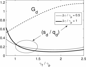
Figure 1: Parameters $G_{d}$ and $s_{d}/q_{d}$ in (15) and (16) as functions of the thermal spread of the plasma $\gamma_{T}/\gamma_{p}$, plotted for two representative values of the relative shift $\Delta\gamma/\gamma_{p}=0.5,\,1$ between the centers of the electron and positron distributions; see (11). The ellipse indicates grouping of the two $s_{d}/q_{d}$-curves, to distinguish them from the $G_{d}$-curve.

Two comments are in order about the coefficients in the NLSE (13). First, Eqs. (15) and (16) and Fig. 1 explicitly demonstrate the point that we have mentioned earlier. Namely, the same nonlinear process of resonant interaction between relativistic charged particles and packets of Langmuir waves gives rise to both nonlinear terms: the purely cubic one (proportional to to $q_{d}$) and the nonlocal one (describing nonlinear Landau damping and proportional to $s_{d}$). Thus, a comprehensive analysis of the NLSE (13) is to take into account both these terms.  Second, it follows from Fig. 1 of MGP00 that for the considered ranges of thermal spread $\gamma_{T}/\gamma_{p}$ and relative shift $\Delta\gamma/\gamma_{p}$ of the positrons’ and electrons’ distribution functions, $q_{d}$, and hence $q$ in (13), is positive. Since also $G>0$ (see (14) and Fig. 1 above), then the NLSE (13) is of the so-called focusing type ($G\cdot q>0$). It is widely known that in the focusing, purely cubic NLSE, solitons can form from an appropriate — i.e., localized, — initial state.

MGP00 exhibited and analyzed the soliton solution of the NLSE without taking into account the effect of nonlinear Landau damping. This approximation had to be made since no analytical solution of that equation with the nonlinear Landau damping terms is known. Physically, this approximation is justified only when the nonlinear Landau damping term, $\propto s$, is so small compared to the nonlinear term, $\propto q$, that it does not have the chance to affect the evolution of the Langmuir wave’s envelope over typical times considered. However, we will show below for reasonable parameters of pulsar plasma, this assumption does not necessarily hold; hence the effect of nonlinear Landau damping over such sufficiently long times cannot be neglected.

Our study extends that of MGP00 in two ways. First, obviously, we take into account the nonlinear Landau damping term by carrying out numerical simulations of the NLSE (13). Second, and more importantly, we study the evolution of a disordered initial state instead of a soliton and find a striking difference between these two evolutions. It should be mentioned that the approximate evolution of the NLSE soliton under the effect of a small nonlinear Landau damping has been considered in a number of studies: see, e.g., Weiland et al. (1978); Flå et al. (1989); Ehsan et al. (2009); Chatterjee & Misra (2015); Misra et al. (2017); Chaudhuri & Roy Chowdhury (2018). They all have found that this perturbation leads to the decay and acceleration of the soliton. In contrast, we will demonstrate that due to the interaction of the intense pulse (which, as we will argue, is a soliton) with the surrounding field, the pulse’s amplitude will grow to significantly exceed that of the said field.

With this motivation, we will now proceed to nondimensionalizing the NLSE (13) with nonlinear Landau damping, so as to later solve it numerically.

5 Nondimensionalization of Eq. (13)

We begin by nondimensionalizing the space variable in the MFR:

$$\chi=l\,\theta\,x,$$ (17a)

where $$x \theta l$$ is the nondimensional space variable, factor is to be defined shortly, and the characteristic scale is defined as:

$$l=c/\omega_{p}=\lambda_{p}/(2\pi)\,,$$ (17b)

with $\lambda_{p}$ being the spatial period of Langmuir waves in the MFR, and the plasma frequency $\omega_{p}$ is given by Eq. (8). The parameter $2\pi\,l$ is of the same order of magnitude as the Langmuir spatial period $\lambda_{p}$ (in the MFR) at some intermediate location of the plasma cloud (see section 3). Therefore, factor $\theta/(2\pi)$ in (17a) characterizes the ratio of spatial scales of the Langmuir wave envelope to the Langmuir period $\lambda_{p}$. In what follows we will consider this ratio to be on the order of $10^{2}\ldots 10^{3}$, whence $\theta=10^{3}\ldots 10^{4}$.

We would like to stress that the above assumption about the range for $\theta$ does not impact the main conclusion of our study, for two reasons. First, as we will show below, a value of $\theta$ results merely in a ball-park estimate of the maximum nondimensional simulation time, while the freedom to adjust the nonlinearity coefficient in the nondimensional equation will still allow us to observe the important changes in the electric field’s evolution. Second, it is realistic to assume that there exists a wider range of $\theta$ values than what we assumed above; this simply corresponds to the envelope of the initial electric field having a wider range of spatial scales. Then, for a given amplitude of the electric field’s envelope (i.e., for a given magnitude of nonlinear terms in Eq. (13)), only those of its fluctuations whose wavelength fall into a narrow(er) range of values will exhibit the phenomenon of pulse formation described below. In other words, the fluctuations with the spatial scale of interest to us will be selected by the governing Eq. (13) and not by our assumption of the range of $\theta$ (as long as that range is sufficiently broad).

In addition to an uncertainty in the value range of our nondimensional parameters that occur due to an uncertainty of the scaling parameter $\theta$, there is also a (much smaller) uncertainty due to these parameters’ dependence on the height $R$ above the pulsar surface where the coherent radiation is emitted. In (12c) we estimated that this occurs around 500 km above the surface. Correspondingly, $R_{50}\sim 1$, as defined after Eq. (6), and this value is to be used to estimate the plasma frequency $\omega_{p}$ in (8) and hence the parameter $l$ in (17b). For other values of $R_{50}$, one has $l\propto R_{50}^{1.5}$. We will use this fact in section 6.1 below.

Next, we normalize $E_{\|}$ to a typical magnitude of the electric field, $E_{0}$, at a location where the two-stream instability sets in in the cloud of secondary plasma (see (12a)):

$$E_{\|}=E_{0}\,u;$$ (18)

thus $u$ is the nondimensional electric field. Note that by this definition, $u=O(1)$ initially.

Finally, we introduce the nondimensional time, $t$, via

$$\tau=\frac{(l\theta)^{2}}{G}\,t=\frac{4\theta^{2}}{\gamma_{p}^{2}\omega_{p}\,G_{d}}\;t,$$ (19)

where we have used formula (17b) and the relation (14). Then, upon dividing through by $G/(l\theta)^{2}$, Eq. (13) attains the form:

$$i\frac{\partial u}{\partial t}+\frac{\partial^{2}u}{\partial x^{2}}+Q\,u\left(|u|^{2}+\frac{s}{\pi q}\;-\int\frac{|u(x^{\prime},t)|^{2}\;dx^{\prime}}{x-x^{\prime}}\,\right)\,=\,0.$$ (20)

where using Eqs. (14) and (15) we have:  $Q=qE_{0}^{2}(l\,\theta)^{2}/G=\big{(}2E_{0}\theta\,e^{2}/(\gamma_{p}^{2}m_{e}c\omega_{p})\big{)}^{2}\,q_{d}/G_{d}$. The initial condition to this equation has, by design, the nondimensional magnitude and spatial scale of order one: $|u|\sim 1$ and $|u|/|u_{x}|\sim 1$.

Let us now estimate the maximum nondimensional simulation time. First, the dimensional prototype of that time, $\tau_{\max}$, is that needed for a Langmuir wave packet to travel, within the cloud of secondary plasma, a length ${\Delta R}$, where the Langmuir turbulence is sufficiently strong (i.e. the nonlinear and dispersive terms in (13) significantly affect the wave packet’s evolution). As estimated in Eq. (12b), ${\Delta R}\sim 500$ km. Since that length is referenced in the OFR while $\tau$ is measured in the MFR, the Lorentz factor $\gamma_{p}\sim 10^{2}$ (see Eq (7)) needs to be accounted for; thus

$$\tau_{\max}\approx\frac{\Delta R}{c\,\gamma_{p}}\sim 10^{-5}{\rm s}.$$ (21a)

Using now relation (19), where $$G_{d}\sim 1 \omega_{p}\sim 4\times 10^{9} P\sim\dot{P}_{-15}\sim\kappa_{4}\sim R_{50}\sim 1$$ (see Fig. 1), and an estimate s^-1 for a typical pulsar with (see Eq. (8))), one obtains that:

$$t_{\max}\sim 10^{8}/\theta^{2}\,\sim\,1\ldots 10^{2}.$$ (21b)

Here the last estimate follows from our earlier assumption $\theta=10^{3}\ldots 10^{4}$.

Now, as we will demonstrate in the next section, the hallmark of the evolution of a Langmuir wave packet governed by Eq. (13) is the formation, out of an initially disordered state, of an intense pulse with an internal structure. In light of this, we should consider such values of nonlinear parameters $Q$ and $(s/q)$ in the nondimensional Eq. (20) that result in such formation over the times estimated in (21b). As for parameter $(s/q)$, which characterizes the strength of nonlinear Landau damping relative to the purely cubic nonlinearity (and does not depend on details of nondimensionalization; see (15) and (16)), its size can be estimated from Fig.1. For moderately large values of the thermal spread, $\gamma_{T}/\gamma_{p}\sim 1\ldots 2$, one finds the size of the nonlinear Landau damping term relative to the size of the purely cubic nonlinear term fall in the range

$$s/q\,=\,s_{d}/q_{d}\,=\,0.05\ldots 0.2.$$ (22)

On the other hand, it is not possible to estimate the correct order of magnitude of the nondimensional parameter $Q$ in (20) based on physical grounds, because one does not have an estimate for the unknown electric field $E_{0}$. Therefore, we simply had to use trial and error to find a range of values of $Q$ such that, for $(s/q)$ being in the range (22), the times of intense pulse formation are in the range (21b). As we will demonstrate in the next section, such $Q$ have the magnitude $O(1)$.

6 Numerical simulations of Eq. (20)

In order to solve Eq. (20), we used a numerical method recently proposed in Lakoba (2016). This method combines the leap-frog (LF) solver with the idea of the integrating factor (IF) method and hence will be referred to as IF-LF. For the reader’s convenience we present its details in Appendix A. The non-physical parameters of the simulations, such as time step $\Delta t$ and mesh size $\Delta x$, are also listed there.

As we mentioned in the Introduction and in section 3, the nonlinear evolution of Langmuir waves commences at a distance of around 200 km from the pulsar; see text before (12a). It is reasonable to assume that the electric field there, amplified by the two-stream instability, does not have any regular structure but is, instead, disordered. Therefore, we take the initial condition $u(x,0)$ for the envelope of the Langmuir wave in Eq. (20) in the form of a mixture of a constant and a zero-mean random field. In the simulations we vary both the ratio $r$ of these two parts in the mixture and the correlation length $l_{\rm corr}$ of the random part, since the actual range of these physical parameters in the plasma is not known. Thus:

$$u(x,0)=(1-r)+r\,\int\frac{\exp[-0.5(k/k_{\rm corr})^{2}-ikx]}{\sqrt{\sqrt{\pi}\,k_{\rm corr}}}\;\widehat{w}(k)\,dk;$$ (23a)

where $$k_{\rm corr}=2\pi/l_{\rm corr} \widehat{w}$$ and is a white noise in Fourier space:

$$\langle\hat{w}^{*}(k_{1})\hat{w}(k_{2})\rangle=2\boldsymbol{\delta}(k_{1}-k_{2}),\qquad\langle\hat{w}(k_{1})\hat{w}(k_{2})\rangle=0;$$ (23b)

here $\langle\cdots\rangle$ stand for the ensemble averaging and $\boldsymbol{\delta}$, for the delta-function.

As we have announced in the previous section, we will be interested in an evolution that leads to the emergence of an intense pulse from an initially disordered state (23b). Due to nonlinear Landau damping, spectral components of the evolving electric field’s envelope shift off-center during the evolution, which causes the forming pulse to move (with non-zero acceleration) in the reference frame of Eq. (20). Modeling realistically such a moving pulse would require a very large spatial computational domain, which is out of reach for our computational resources. We therefore resorted to a common numerical trick: We impose periodic boundary conditions on a finite-length domain, thereby modeling repeated passing of a pulse (or some disordered field) through this domain. For the simulations reported in the main part of this work, we restricted our consideration to the nondimensional value $L=40\pi\approx 126$. In Appendix B we demonstrate that increasing the length of the computational domain does not alter our principal finding, which is the formation of an intense pulse from an initially disordered field due to nonlinear Landau damping (see next section). Moreover, we explain there why the periodicity of the boundary conditions does not affect this formation at all, as long as the domain is sufficiently long.

Thus, in our simulations we have four physical parameters that we varied: ratio $r$ of the random and constant components in the initial state of the field (23b); correlation length $l_{\rm corr}$ of the random component there; nonlinear Landau damping coefficient $(s/q)$, and the cubic nonlinearity coefficient $Q$ in (20).

6.1 Main results

6.1.1 Formation of an intense pulse due to nonlinear Landau damping

We will now present the first of the two key findings of this study: the formation, due to nonlinear Landau damping, of a long-living intense pulse from a disordered initial field. At this point, it is appropriate to remind the reader (see, e.g., Solli et al. 2007; Fedele et al. 2010; Lakoba 2015; Agafontsev & Zakharov 2015; Gelash & Agafontsev 2018) that in the purely cubic NLSE, intense pulses do routinely emerge from a disordered state, with this emergence occurring on a time scale that is several times faster than $O(1/Q)$. However, they dissolve about as quickly as they emerge. (Typically, the greater the pulse’s amplitude, the shorter time it “lives".) In contrast to this “flickering pulse" behavior in the purely cubic NLSE, in the NLSE with nonlinear Landau damping an intense pulse forms over a time on the order of $O(1/Q)$ and then propagates stably over a long time without showing any sign of decay. We will now present a detailed description of this process.

A typical evolution of the field and its Fourier spectrum, representative of such a process, is illustrated in Fig. 2. At first, there is a transitional time interval (approximately until $t=40$ in the case shown in Fig. 2), during which the field and its spectrum remain statistically similar to the initial ones. Some moderately intense field fluctuations occur during that time, but they keep on quickly dissolving, thus mimicking a disordered field evolution in the purely cubic NLSE described in the previous paragraph. Then, a new phenomenon appears due to nonlinear Landau damping: Within a short period (somewhere in $40\lesssim t<45$ in the case of Fig. 2 (b)), an intense pulse begins to form and, most importantly, no longer dissolves back into a disordered state. As the pulse keeps on becoming taller and narrower, its spectrum develops a secondary peak (circled in Fig. 2), which begins to shift exceedingly fast away from the original central wavenumber of the field. This shift of the field’s spectral components occurs due to nonlinear Landau damping, whereby energy from Fourier harmonics with $k>0$ is transferred to those with $k<0$ (for $(s/q)>0$ in Eq. (20)). This stage, where the pulse “matures", takes a relatively short time (approximately corresponding to $45<t<55$ in the case of Fig. 2), after which the growth and narrowing of the pulse in physical space slow down and then cease. In the “mature" stage, the only two effects of the nonlinear Landau damping on the pulse evolution are: the accelerated moving (in the reference frame of Eq. (20)) in the physical space and the moving of the secondary peak in the Fourier space. For the parameters used in this simulation, one is able to reliably observe this “mature" stage of the pulse evolution only for a relatively short time. The reason is that by $t\sim 65$, the secondary peak has already moved too close to the left edge of the computational spectral domain, so that spectral components of the solution near $k\approx-k_{\max}$ have increased considerably above the initial noise level. To prevent those components from invalidating the numerical solution, we stopped simulations when the Fourier amplitude of those components would reach (an arbitrarily chosen) value $10^{-4}$. A detailed observation and examination of the “mature" stage of the pulse evolution is possible either for a wider computational spectral domain (see below) or for smaller values of $Q$ or $(s/q)$. However, the latter would increase the time needed for the pulse formation to several hundred units, which is beyond the physically relevant range (21b), and therefore is not presented here.

The unbounded widening of the solution’s spectrum presents an issue for the validity of that solution not only from the numerical, but also from a physical perspective. Indeed, one of the key assumptions under which the governing equation (13) is valid is that the characteristic scale of the initial perturbation in the plasma must be much greater than the Langmuir wavelength. After Eqs. (17b), we assumed that the ratio of these two spatial scales, denoted there as $\theta/(2\pi)$, is on the order of $10^{2}\,\ldots\,10^{3}$. When the solution’s spectrum widens $M$ times, its characteristic spatial scale decreases by the same factor. Therefore, the governing model remains valid only as long as $\theta/(2\pi M)\gg 1$, whence one must require that the spectrum widening factor be limited by $M<10^{2}$. If the initial (nondimensional) spectral half-width of the solution is $k\sim 2$, as in Fig. 2, then the solution will remain physically valid as long as the separation between the secondary and primary spectral peaks does not exceed $\sim 100$ units.

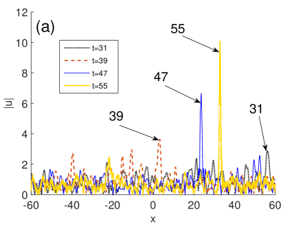
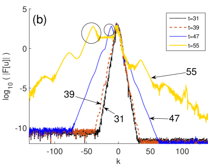
Figure 2: (Color online)  Field (a) and spectrum (b) of the solution of Eq. (20) with the initial condition (23b) for $Q=0.25$, $r=1$, $l_{\rm corr}=\pi$, and $s/q=0.05$. (Only part of the spectral domain is shown for better visibility of details.) The arrows mark the times at which the solution is plotted. The circles in panel (b) mark the “solitonic" part of the pulse, corresponding to the intense peak, as discussed in the text.

A closer examination of the solution’s Fourier spectrum reveals that while the remnants of the original spectral peak remain “noisy" (i.e., jagged in Fig. 2), the secondary, “breakaway" peak, corresponding to the intense pulse, is smooth and has clearly seen exponentially decaying tails. This leads us to hypothesize that the created pulse is a soliton of the perturbed NLSE (20). Creation of a long-living intense pulse out of a disordered initial condition has been reported before (Jordan & Josserand 2001; Genty et al. 2010) for the generalized NLSE. However, in those cases, the size of the perturbation, interpreted as the difference between the given NLSE and the purely cubic one, was not small. Namely, either the nonlinearity was considerably different from cubic (Jordan & Josserand (2001) and references therein) or a higher-order dispersion term in the cubic NLSE was of order one (Genty et al. 2010). Moreover, there are two differences in our observation of the pulse’s emergence compared to such observations in those earlier studies. First, our Eq. (20) contains only a small perturbation to the NLSE: $(s/q)\lesssim 0.1$. This makes the second difference even more surprising: in strongly non-cubic generalized NLSE considered earlier by Jordan & Josserand (2001), the time that it took an intense pulse to emerge was about two to three orders of magnitude greater than in the slightly perturbed NLSE (20). A theoretical explanation of these differences, as well as of the very fact that a small nonlinear Landau damping causes the emergence of an intense pulse from a disordered state, remains an open problem. At a qualitative level, the emerging pulse appears to harvest energy from the surrounding field. However, what triggers the event after which the pulse begins doing so, and why its growth eventually ceases, is unknown.

Thus, to summarize our first key finding: A small nonlinear Landau damping leads to two qualitative changes of a disordered initial field. First, unexpectedly, it causes formation of an intense pulse that exists over a long time (at least as long as the model (13) remains physically and numerically valid). Second, expectedly, it leads to an (accelerated) shift of that pulse in the spectral domain towards lower wavenumbers (for $(s/q)>0$).

6.1.2 Internal structure of the pulse, and features of radiation

Our second key finding concerns the wavelength of the radiation emitted by the plasma where an intense pulse has formed due to the mechanism described above. The intense pulse creates a ponderomotive force which prevents the charge bunch from collapsing. The ponderomotive force is $\propto\nabla|E_{\|}|^{2}$, which, when used in conjunction with the Poisson equation and restricted to the one-dimensional motion along magnetic field lines (see section 1), gives the charge density across the pulse to be proportional to $\partial^{2}|E_{\|}|^{2}/\partial x^{2}$ (see MGP00). The charge density, in turn, is a coherent structure bounded by the width of the intense pulse, which moves along curved magnetic field lines to produce coherent curvature radiation. To illustrate that finding, in Figs. 3 and 4 we compare the quantity $\partial^{2}|u|^{2}/\partial x^{2}$ (recall $u$ is the nondimensional electric field given by Eq.(18)), in the initial state (Fig. 3) and in a state where a pulse has formed (Fig. 4). The simulation was run for the same parameters as in Fig. 2, except that, in order to resolve a high-wavenumber ripple in Fig. 4, we used a three-time wider spectral window and a correspondingly smaller time step (see Appendix A). Since the time of formation of an intense pulse is sensitive to the initial condition (and hence the computational spectrum), in Figs. 3 and  4 it is different from that in Fig. 2.

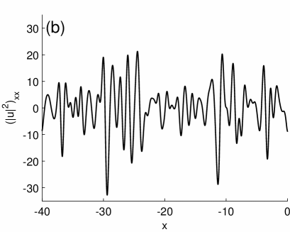
Figure 3: Quantities proportional to the intensities of the electric field (a) and radiation (b) in the initial state ($t=0$). Simulation parameters are the same as in Fig. 2, except that the computational spectrum is three times broader. Only part of the spatial computational domain is shown for clarity.

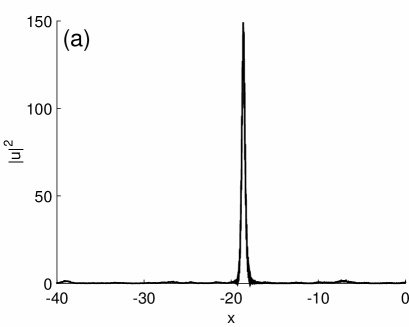
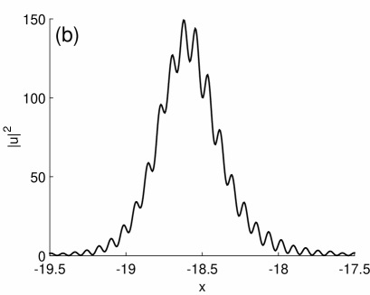
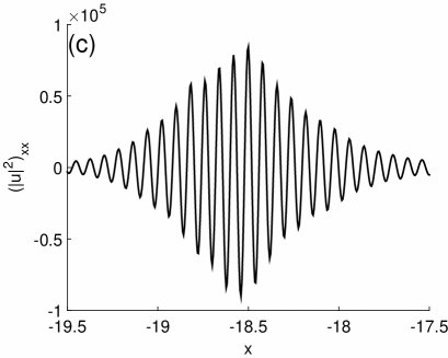
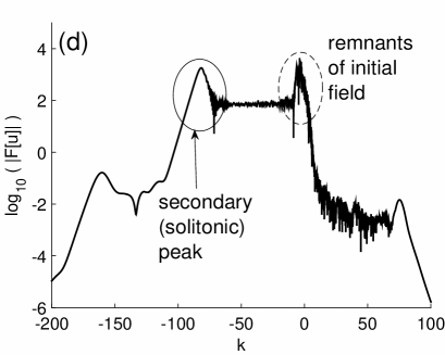
Figure 4: Same simulation as in Fig. 3, but at $t=66$, after an intense pulse has formed and “matured". Panel (a) is a counterpart of that in Fig. 3. Note that most of the computational domain is occupied by the field whose intensity is some two orders of magnitude smaller than that of the main pulse. Panel (b) is a close-up of (a) focusing on the vicinity of the pulse. Panel (c) is a counterpart of Fig. 3(b). Panel (d) shows part of the Fourier spectrum of the numerical solution.

A comparison of Fig. 3(b) and Fig. 4(c) shows a more than three-order of magnitude increase of the radiation’s intensity. It is important to note that this increase occurs due to two separate reasons: first, formation of a pulse whose amplitude, i.e. $\max|u|$, is an order of magnitude greater than that of the initial field (compare Fig. 3(a) to Fig. 4(a)), and second, existence of a highly oscillatory ripple “on top" of the pulse (see Fig. 4(b)). The spatial period of this ripple is about an order of magnitude smaller than unity, which adds approximately two orders of magnitude to the size of the second derivative of $|u|^{2}$ (see Fig. 4(c)).

The wavelength of the ripple $\delta x_{\rm ripple}$ “on top" of the intense pulse is explained by the spectrum of the field: see Fig. 4(d). Specifically, the “bulk" of the pulse corresponds to the “solitonic" spectral peak located at $k\approx-80$ in that figure. On the other hand, “remnants" of the initial field have $k\approx 0$. Thus, the intensity of the superposition of these two parts of the field, i.e.

$$|u|^{2}\approx\big{|}A_{1}e^{-i80x}+A_{2}e^{i0x}\big{|}^{2}=(|A_{1}|^{2}+|A_{2}|^{2})+2|A_{1}||A_{2}|\cos(80x+\phi),$$ (24)

has the approximate wavelength of the ripple as, $\delta x_{\rm ripple}=(2\pi)/80\approx 0.07$. (In (24), $A_{1},A_{2}$, and $\phi$ are some constants.) This wavelength is the smallest scale of a coherent structure inside the intense solitonic pulse and is clearly visible in Fig. 4(b) and 4(c). In section 7 we will demonstrate that while this structure is “short-lived" compared to the pulse itself, it still can be a source of coherent emission.

Thus, we have found two types of structures that emerge from an initially disordered state of electric field in the pulsar plasma:  (i) an intense pulse of the envelope of Langmuir waves and  (ii) a “ripple" on top of this pulse. We will conclude this subsection with an estimation of their characteristic spatial scales and the corresponding frequencies that they can emit. We will begin with the intense pulse and use the parameters reported for, and shown in, Fig. 4. In dimensional units, the width of the pulse, $\delta\chi_{\rm pulse,\,\circ}\,$, in the OFR can be estimated as follows. First, since the nondimensional time that it takes the intense pulse to form is $t\approx 60\sim 100$, then (21b) implies that $\theta\sim 10^{3}$. Using this value and $\omega_{p}\sim 4\times 10^{9}$ s^-1 in Eqs. (17b) and a value $\gamma_{p}\sim 10^{2}$ to convert between the OFR and MFR variables, one obtains:

$$\delta\chi_{\rm pulse,\,\circ}=\delta\chi/\gamma_{p}=l\theta\delta x_{\rm pulse}/\gamma_{p}\sim 3\times 10^{8}~{}~{}{\rm m\cdot s}^{-1}/(4\times 10^{9}~{}~{}{\rm s}^{-1})\cdot 10^{3}\cdot 1/10^{2}\sim 70~{}~{}{\rm cm}.$$ (25a)

This corresponds to the radiation’s frequency of about  $$c/\delta\chi_{\rm pulse,\,\circ}\sim 400 R_{em} 500 \delta x_{\rm ripple}$$ MHz and thus falls in the mid-range of the spectrum of observed pulsar coherent radio emission, which extends from several tens of MHz to a few GHz. Let us note that this estimate can go down by a factor of two or so if one allows for the possibility that the radiation is emitted from altitudes that are lower than the value of km assumed in (12c); see the paragraph before Eq. (18). Similarly, since the nondimensional wavelength of the ripple on top of the pulse is seen to be about an order of magnitude smaller, then

$$\delta\chi_{\rm ripple,\,\circ}\sim 7~{}~{}{\rm cm},$$ (25b)

and the corresponding frequency is about 4 GHz. In the next subsection we will show that both frequencies following from estimates (25b) may go down by about an order of magnitude if one assumes a higher value of the nonlinearity coefficient. In section 7 we will further discuss the relevance of our numerical observations to the problem of coherent emission by change bunches in plasma.

Having presented our main findings, we now describe how the formation of an intense pulse is affected by the physical parameters of the governing equation (20).

6.2 Dependence of pulse formation on $Q$

Predictably, as one increases $Q$ without changing other parameters in (20), the field evolution due to nonlinear terms (both purely cubic and Landau-damping ones) occurs faster, and the time required for the pulse formation decreases. This is illustrated in Table 1, where we list the times $t_{4\times}$ that it takes the pulse’s amplitude, $\max_{x}|u|$, to exceed an arbitrarily set threshold of 4, which is four times the average amplitude of the initial state (23b). These times are seen to decrease with the increase of $Q$, as expected. At the same time, we found that the spatial scale of the intense pulse is not significantly affected by $Q$. This fact will play a role in the forthcoming estimate of the dimensional wavelength and frequency of the coherent radio emission that such a pulse can generate.

	0.3	0.4	0.5	0.6	0.7	0.8	0.9	1.0	1.1	1.2	1.3	1.4	1.5
0.05	40	30	20	12	6.1	5.8	4.0	3.0	3.4	2.9	2.0	1.8	1.5
0.10	21	11	7.5	5.5	4.4	3.5	3.0	3.5	2.8	2.1	2.0	1.6	1.5

Table 1: Evolution times $t_{4\times}$ that it takes the pulse’s amplitude to exceed four times the average amplitude of the initial state. The initial condition (23b) has parameters $r=0.9$ and $l_{\rm corr}=\pi$. All simulations use the same seed of the random number generator, leading to the same initial pulse profile. Since details of the pulse evolution depend on the (randomly chosen) initial profile, the times $t_{4\times}$ are listed only to two significant figures, which suffices to illustrate the general trend.

Namely, we can accept that the distance $\Delta R$ that it takes for the instability in the secondary plasma cloud to lead to formation of an intense pulse is given by (12b); then the dimensional time of pulse formation continues to be given by (21a). In such a case, the decrease in the nondimensional time, seen in Table 1 as $Q$ increases, implies that $\theta$ takes on values from the upper part of its range, e.g., $\theta\sim 10^{4}$: see (21b). Now, for a greater $\theta$, a given nondimensional spatial scale corresponds to a greater dimensional scale: see (17b). Thus, as $Q$ increases, the dimensional scale of both the solitonic pulse and the fine structure on top of it can go up by an order of magnitude compared to (25b). Consequently, the frequencies of the coherent emission can be found in the range from several tens to several hundreds of MHz for the pulse and the “ripple", respectively.

We should be careful to note that this is only one interpretation of the observed decrease of $t_{4\times}$ with $Q$; other interpretations may be possible. For example, one can assume that the increase of $Q$ implies that the Langmuir turbulence in the plasma cloud is so strong that the formation of an intense pulse occurs not over 500 km, as in (12b), but much sooner, say, over 100 km. In this case, both $\theta$ in (21b) and $R_{50}$ in (8) would change compared to their values in (25b). However, a more detailed analysis of such a possibility is outside the scope of this study.

Coming back to Table 1, we note that for the two different values of the nonlinear Landau damping coefficient $(s/q)$, the most pronounced decrease of $t_{4\times}$ occurs for a higher range of $Q$ values for the smaller $(s/q)$: for $Q\in(0.4,\,1.0)$ for $(s/q)=0.05$, and for $Q\in(0.3,\,0.5)$ for $(s/q)=0.10$. For both values of $(s/q)$, the decrease of $t_{4\times}$ significantly slows down for $Q$ values above those respective ranges.

In the next subsection we will discuss other changes in the pulse evolution that occur with changing the nonlinear Landau damping coefficient $(s/q)$.

6.3 Dependence of pulse formation on $(s/q)$

The expected effect of varying the nonlinear Landau damping coefficient is that the formation time of an intense pulse decreases as $(s/q)$ increases. However, and perhaps less expectedly, an increase of nonlinear Landau damping beyond a certain point begins to have less effect on the speed of the pulse formation. This can be seen from the data reported for larger values of $(s/q)$ in Table 2. Moreover, at least four other changes occur with the increase of nonlinear Landau damping. First, the shape of the pulse becomes visibly asymmetric, with a “tail" forming behind the pulse; see Fig. 5(a). Second, this change in the shape is accompanied by a decrease of the amplitude of the “matured" pulse; compare Fig. 5(a) to Figs. 4(a,b). Third, the intensity of the radiation emitted by the pulse decreases, whereas its wavelength increases: compare Fig. 5(b) to Fig. 4(c) and note that respective horizontal and vertical scales are different. These effects are manifested in the Fourier space as follows:  (i)  the spectral peak corresponding to the intense pulse is now much less prominent over a spectral “plateau" that is observed immediately on its right side, and  (ii) “remnants" of the initial field with spectral components near $k=0$ have been considerably reduced for the larger value of $(s/q)$. Thus, the spectrum of the field is considerably narrower for the larger values of nonlinear Landau damping. Finally, and perhaps unexpectedly, the shift of the spectrum occurs much slower for larger values of $(s/q)$. Specifically, the pulse shown in Fig. 5 for $(s/q)=0.15$ forms around $t=25$, whereas that shown in Fig. 4 for $(s/q)=0.05$ forms around $t=50$. The spectrum of the latter pulse approaches the left edge of the computational domain (i.e., $-k_{\max}\approx-600$ in this case) already for $t=75$, by which time the numerical solution becomes invalid (see the beginning of section 6). On the contrary, the spectrum of the pulse for $(s/q)=0.15$ is seen not to reach even one half of the computational spectral window by $t=100$.

	0.01	0.02	0.04	0.06	0.08	0.10	0.13	0.16	0.20
$(1;\;\pi)$	14	8.0	4.5	4.1	3.5	3.4	3.1	3.0	2.6
$(1;\;1)$	$>100$	65	32	27	16	12	12	9.2	9.4
$(2;\;1)$	$30$	14	11	7.0	6.1	4.6	3.5	2.5	4.4

Table 2: Dependence of the times $t_{4\times}$ on the nonlinear Landau damping coefficient. The initial condition for each simulation is the same and has $r=0.9$.

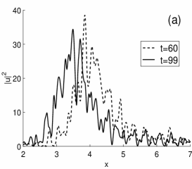
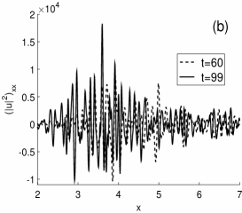
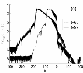
Figure 5: Same simulation parameters as for Fig. 4, but for a larger value of nonlinear Landau damping $(s/q)=0.15$. Solution at two times are shown to illustrate slow evolution of the field’s spectrum for larger values of $(s/q)$. The two times are chosen so that the locations of the intense pulse would nearly coincide, to facilitate visual comparison of the two pulses. Only part of spatial and spectral domains is shown for better visibility.

For completeness, we also verified that as $(s/q)$ increases to become of order one, a pulse no longer forms. Instead, a “step" with an oscillatory “tail" is formed. The spectrum of this solution is approximately flat at the top, with the top’s width increasing with time.

6.4 Dependence of pulse formation on $l_{\rm corr}$

The effect of the spatial scale of the initial condition on the field evolution is predictable, at least withing some range. Namely, as $l_{\rm corr}$ decreases, the effect of the dispersive term $u_{xx}$ in Eq. (20) increases compared to that of the nonlinear term. Thus, having a smaller $l_{\rm corr}$ in the initial condition is, essentially, similar to having a smaller $Q$: it delays pulse formation. This is confirmed by comparing the first and second lines in Table 2, which show the effect of decreasing $l_{\rm corr}$. In comparison, the third and second lines of the same Table show that a similar effect of pulse formation delay occurs when $Q$ is decreased, as has already been noted in section 6.2.

6.5 Dependence of pulse formation on $r$

Finally, we investigated how the “degree of randomness" of the initial state affects the pulse formation. Initially, we expected that the formation times would increase with the share of the random component in the initial state. However, in numerical experiments we observed that while those times indeed initially increase with $r$, they reach a maximum around $r=0.5$ and then begin to decrease. Representative results are shown in Fig. 6(a). We observed qualitatively the same results for several other values of parameters $Q$ and $(s/q)$ than reported in Fig. 6, as well as for a different initial random state (controlled by the seed of the random number generator in the numerical code).

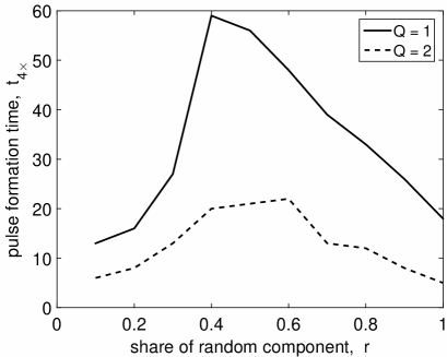
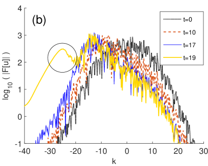
Figure 6: (a)  Typical dependence of the pulse formation time on the share of the random component in the initial field. Parameters are: $l_{\rm corr}=1$ and $(s/q)=0.05$. To generate the random part of the initial condition, we used the same seed of the random number generator for all $r$.  (b)  (Color online)  Fourier spectra illustrating the evolution of an initial random state ($r=1.0$) into an intense pulse, as explained in the text; $Q=1$. Only part of the spectral domain is shown for better visibility of details.

In Fig. 6(b) we show different stages of the field evolution, which were found to be similar for all $r\gtrsim 0.4$. Initially, nonlinear Landau damping leads mostly to a (rather slow) shift of the field’s Fourier spectrum, with only minor changes of the spectrum’s shape; compare the curves for $t=0$ and $t=10$. In physical space, the field appears disordered during that stage. Then, the spectrum begins to become noticeably narrower and asymmetric; it is shown at $t=17$, which is shortly before the formation of an intense pulse. (Incidentally, the spectral narrowing corresponds to the increase of the correlation length of the field, and, according to the previous subsection, this facilitates the pulse formation.) Finally, an intense pulse forms within a relatively short time interval; see the curve for $t=19$ in Fig. 6(b). In the spectrum, the formation of a pulse corresponds to the emergence of a secondary peak around $k\approx-30$, marked with a circle; compare it with Figs. 2(b) and 4(d). Once the pulse is formed, its height and width remain almost unchanged, until the numerical solution loses its validity due to a significant part of the spectrum shifting near the left edge of the spectral window (see section 6.1.1).

7 Summary and Discussion

We have addressed the open problem of explaining a mechanism of coherent curvature radio emission by the electron–positron plasma in pulsar magnetosphere. As the mathematical model of this phenomenon we considered the generalized nonlinear Schrödinger equation (NLSE) proposed by Melikidze et al. (2000) (MGP00), which includes effects of group velocity dispersion, nonlinearity of electric susceptibility, and resonant interaction between Langmuir waves and plasma particles (nonlinear Landau damping). In the absence of nonlinear Landau damping, the purely cubic NLSE can, in principle, support solitons, which in the plasma would be manifested as charge bunches that propagate stably and therefore are capable of emitting coherent radiation. However, formation of solitons in the purely cubic NLSE requires that initially, the Langmuir wave have the envelope that is either localized or consists of several well-separated localized “bumps". It is only then that the emerging charge solitons can maintain their shape for a sufficiently long time to radiate coherently. There is no reason to expect that such a special initial condition of Langmuir waves would exist in a disordered pulsar plasma. Then, it is known (see section 6.1.1) that evolution of a disordered initial state in the purely cubic NLSE leads to an ensemble of strongly interacting pulses, which constantly appear, disappear, and change their shape due to the interaction. Such a disordered, in both time and space, ensemble of pulses cannot be expected to emit coherently.

Motivated by this inability of the purely cubic NLSE to identify a candidate mechanism of coherent emission, we numerically solved the NLSE with the nonlinear Landau damping term, as derived by MGP00. We found that for a range of realistic values of pulsar parameters, the presence of nonlinear Landau damping leads to the formation of an intense, soliton-like pulse out of an initially disordered Langmuir wave. Such a stable pulse can emit coherently and thus is a reasonable candidate as a source of coherent radio emission. However, an analytical explanation of this emergence of a long-living intense pulse remains an open problem.

Let us point out a key difference between this result and the results of earlier studies (Weiland et al. 1978; Flå et al. 1989; Ehsan et al. 2009; Chatterjee & Misra 2015; Misra et al. 2017; Chaudhuri & Roy Chowdhury (2018)), which considered the effect of nonlinear Landau damping on an isolated soliton. Those earlier studies found that such a soliton will experience decay and a frequency shift of the carries. Both of these phenomena are consequences of the fact that the nonlocal term in the NLSE (13) describes energy transfer from one side of the pulse spectrum to the other. In contrast, in our simulations, a pulse emerges from an initially disordered state and, during its “maturation" stage, appears to absorbs energy from the surrounding field.

Two important notes about this pulse formation are in order. First, the nonlinear Landau damping coefficient has to fall in a certain range (namely, the lower part of (22)). If it is too high, then the intensity of the emerging pulse is lower, or a stable pulse may even not form at all; see section 6.3. On the other hand, if the nonlinear Landau damping is too low, the pulse may not have the time to form during the stage when the charge density in the plasma cloud is sufficiently large to produce strong radiation; see section 5.

Second, the intense pulse, formed for appropriate values of the nonlinear Landau damping coefficient, has an internal structure whose spatial scale can be about an order of magnitude smaller than the spatial extent of the pulse itself; see Fig. 4(b). In this work we did not undertake an actual calculation of the coherent emission by such stable pulses, containing a large number of charged particles; this clearly requires a separate study. Without such a calculation, one cannot tell to what extent each of these structures: the “bulk" solitonic pulse itself and the finer “ripple" on top of it, contribute to the coherent emission. It appears intuitively plausible that frequencies in the lower end of the observed spectrum (tens to hundreds of MHz) are generated by the pulse as a whole, while frequencies from the higher end (up to several GHz) are generated by the “ripple". This is because the spatial scale of the pulse is about an order of magnitude greater than that of the “ripple"; see sections 6.1.2 and 6.2. However, a calculation of the spectrum emitted by such a two-scale structure of charges remains an open problem.

Let us now demonstrate that while the “ripple" on top of the solitonic pulse keeps changing its shape on a time scale that is small compared to the time scale where such a pulse exists, those changes are still “slow enough" to allow the “ripple" to emit coherently in the range of frequencies estimated in section 6.1.2 (several GHz), and even at lower frequencies. To that end, note that in order for the “ripple" to be a source of coherent radiation, it must exist long enough to guarantee condition (2a). Namely, the time ${\mathcal{T}}_{b}$ over which the shape of this “ripple" remains mostly unchanged must be much greater than the period ${\mathcal{T}}_{c}$ of the coherent radio emission. Let us demonstrate, using the illustrating example of Fig. 4, that this is indeed the case. In Fig. 7 we show that the profiles of both the electric field’s intensity $|u|^{2}$ and the ponderomotive force $|u|^{2}_{xx}$ are mostly preserved over $t\approx 0.01$. Now, if $t\sim 100$ corresponds to $500$ km (see section 5), then ${\mathcal{T}}_{b}\sim 0.01$ corresponds to about $50$ m. Then, condition (2a) implies that the lower limit of frequencies $\omega_{c}$ is about $c/(50\;{\rm m})\sim 10$ MHz. This is consistent (within a two-order of magnitude margin) with the value of several GHz mentioned after estimate (25b).

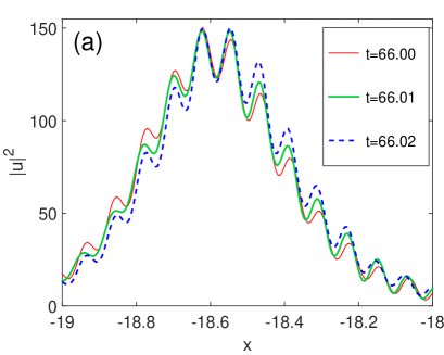
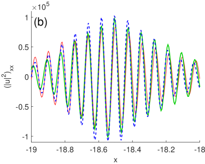
Figure 7: (Color online)  Same quantities as in Fig. 4(b),(c), respectively, but for $t=66.00,\,66.01,\,66.02$. Line colors and styles are as shown in the legend in panel (a). The $x$-window is smaller than in Fig. 4(b),(c) in order to make the details appear more clearly. In both panels, the centers of the pulses at the different times are manually superimposed in order to clearly show the changes of the profile. (If a pulse moves without changing its shape, its does not affect its ability to emit coherently.) We also observed that at $t=66.10$ the profile of the “ripple" has changed completely relatively to that at $t=66.00$; the corresponding curves are not shown in order not to clutter the picture.

Note that since the solitonic pulse itself stably propagates over $t>O(10)$ nondimensional units, there is, for practical purposes, no lower limit from condition (2a) on the frequencies that it, as a whole, can emit coherently.

Finally, let us note that since we had to use periodic boundary conditions in our numerical simulations (see the preamble to section 6), we always observed that only one intense pulse forms as a result of many collisions with smaller pulses. In an actual plasma cloud, where the pulse passes through it only once rather than repeatedly, many well-separated and long-living solitonic pulses may form. Then, taking into account emission by this ensemble of stable charge bunches, as opposed to by a single charge bunch, is yet another open problem.

Appendix A: Numerical method for solving Eq. (20)

We will present this method for equations of the form

$$iu_{t}+{\mathcal{L}}u+{\mathcal{N}}=0,$$ (26)

where ${\mathcal{L}}$ is a linear operator with spatially constant coefficients and ${\mathcal{N}}$ includes all other terms. The generalized NLS (20) is a special case of (26), with ${\mathcal{L}}=\partial^{2}/\partial x^{2}$ and ${\mathcal{N}}$ being the entire nonlinear term. Below we will label the Fourier transform of any quantity with an over-hat:

$$\widehat{u}(k,t)=\frac{1}{\sqrt{2\pi}}\int_{-\infty}^{\infty}u(x,t)\,e^{-ikx}dx,\qquad u(x,t)=\frac{1}{\sqrt{2\pi}}\int_{-\infty}^{\infty}\widehat{u}(k,t)\,e^{ikx}dx.$$

Similarly, $\widehat{\mathcal{L}}\equiv\widehat{\mathcal{L}}(k)$ and $\widehat{\mathcal{N}}\equiv\widehat{\mathcal{N}}(k)$ will denote the Fourier symbols of operators ${\mathcal{L}}$ and ${\mathcal{N}}$, respectively. For example, in (20), $\widehat{\mathcal{L}}=-k^{2}$. Taking the Fourier tranform of (26) yields

$$i\widehat{u}_{t}+\widehat{\mathcal{L}}\widehat{u}+\widehat{\mathcal{N}}=0.$$ (27)

Solving this from $t_{1}$ to $t_{2}$ as a linear inhomogeneous equation yields:

$$e^{-i\widehat{\mathcal{L}}t_{2}}\,\widehat{u}(t_{2})-e^{-i\widehat{\mathcal{L}}t_{1}}\,\widehat{u}(t_{1})=\int_{t_{1}}^{t_{2}}e^{-i\widehat{\mathcal{L}}t^{\prime}}\,i\widehat{\mathcal{N}}(t^{\prime})\,dt^{\prime},$$ (28)

where we have suppressed the obvious $k$-dependence of variables. Thus, the linear term in (26) is accounted for exactly by (28).

In Lakoba (2016) it was proposed to use the leap-frog scheme to discretize the integral on the r.h.s. of Eq. (28) and thereby turn that equation into a numerical method. The leap-frog scheme is well-known to quasi-preserve the $L_{2}$-norm of the numerical solution. Choosing it is, therefore, appropriate for the wide class of equations (26) where this norm is conserved; the generalized NLS (20) with nonlinear Landau damping belongs to that class. It should also be noted that the leap-frog scheme is explicit and hence easy to implement.

Within the leap-frog scheme, two versions of the discretization of the integral in (28) are still possible. As discussed in Lakoba (2016), one of them significantly distorts the solution’s spectrum at the edges of the spectral computational window, while the other does not. For our purposes of modeling nonlinear Landau damping, which constitutes a transfer of energy from higher- to lower-$k$ Fourier harmonics (for $(s/q)>0$), it is essential to have the spectrum undistorted at the edges. Therefore, in this study we used the latter method, which was called IF-LF (integrating factor–leap-frog) in Lakoba (2016). The form of the IF-LF method is Lakoba (2016):

$$e^{-i\widehat{\mathcal{L}}t_{n+1}}\,\widehat{u}(t_{n+1})-e^{-i\widehat{\mathcal{L}}t_{n-1}}\,\widehat{u}(t_{n-1})=2\Delta t\,e^{-i\widehat{\mathcal{L}}t_{n}}\,i\widehat{\mathcal{N}}(t_{n})\,,$$ (29a)

where $$\Delta t$$ is the time discretization step. For the generalized NLS (20) this simplifies to:

$$e^{ik^{2}\Delta t}\,\widehat{u}(t_{n+1})-e^{-ik^{2}\Delta t}\,\widehat{u}(t_{n-1})=2i\Delta t\,\widehat{\mathcal{N}}(t_{n})\,.$$ (29b)

This method has accuracy $O(\Delta t^{2})$ in time; the discrete Fourier transform yields an exponential accuracy in space, provided that the solution with all its derivatives is continuous.

An extra step is now required to turn method (29b) into a useful tool. Namely, if implemented just as above, the method will become numerically unstable over a time $t_{\rm inst}$, which is on the order of a hundred time units for $Q=O(1)$. This numerical instability occurs for low-$k$ Fourier harmonics and is caused by a so-called “parasitic" solution, which is well-known to be engendered by the leap-frog scheme. As discussed in Lakoba (2016), for $Q<0$ this instability is essentially a linear, modulational-type instability. On the other hand, for $Q>0$, the instability is nonlinear and, to our knowledge, was first analyzed in Briggs et al. (1983); Sloan & Mitchell (1986). A method to suppress the instability caused by the “parasitic" solution was demonstrated and extensively tested in Lakoba (2016). It consists of averaging the solution every $t_{\rm stab}$ time units, with $\Delta t\ll t_{\rm stab}\ll t_{\rm instab}$, in a way that distorts the solution by a negligible amount. In this study, we used $t_{\rm stab}=1$. We will now describe the aforementioned averaging procedure which we used to stabilize the numerical solution.

Denote $\widehat{v}_{n}=\widehat{u}_{n}e^{ik^{2}\,t_{n}}\equiv\widehat{u}_{n}e^{ik^{2}\,n\Delta t}$. Note that (29b) is then rewritten as:

$$\widehat{v}_{n+1}-\widehat{v}_{n-1}=2i\Delta t\,e^{ik^{2}\,t_{n}}\,\widehat{\mathcal{N}}(t_{n})\,,$$ (30)

where $\widehat{\mathcal{N}}(t_{n})$ depends on $\widehat{v}_{n}$. Suppose one has computed the solution up to time $t_{n+3}$ inclusively. Using the solution computed in the last eight time steps, do the following. First, find the average at $t=t_{n}$:

$$\widehat{\overline{v}}_{n}=\frac{11}{64}\widehat{v}_{n}+\frac{15}{64}(\widehat{v}_{n-1}+\widehat{v}_{n+1})-\frac{3}{32}(\widehat{v}_{n-2}+\widehat{v}_{n+2})+\frac{1}{64}(\widehat{v}_{n-3}+\widehat{v}_{n+3}).$$ (31a)

One can verify that $$|\widehat{v}_{n}-\widehat{\overline{v}}_{n}|=O(\Delta t^{6}) t=t_{n-1}$$. Next, repeat this for :

$$\widehat{\overline{v}}_{n-1}=\frac{11}{64}\widehat{v}_{n-1}+\frac{15}{64}(\widehat{v}_{n-2}+\widehat{v}_{n})-\frac{3}{32}(\widehat{v}_{n-3}+\widehat{v}_{n+1})+\frac{1}{64}(\widehat{v}_{n-4}+\widehat{v}_{n+2}).$$ (31b)

Finally, use $\widehat{\overline{v}}_{n}$ and $\widehat{\overline{v}}_{n-1}$ to restart the IF-LF method (30) by replacing, on the l.h.s., $\widehat{v}_{n-1}$ with $\widehat{\overline{v}}_{n-1}$ and, on the r.h.s., $\widehat{v}_{n}$ with $\widehat{\overline{v}}_{n}$. As demonstrated in Lakoba (2016), this procedure suppresses the numerical instability while introducing only negligible dissipation to the solution. A logical flow-chart for implementing this stabilizing averaging in Matlab is found at:
http://www.cems.uvm.edu/~tlakoba/recent_publications/stabilization_step_Eq28
_logical_flowchart.txt.

The IF-LF method with a stabilization step based on (31b) needs to use a time step $\Delta t$ satisfying

$$\Delta t<\Delta x^{2}/\pi\equiv\pi/k_{\max}^{2}$$ (32)

in order to guarantee numerical stability of high-$k$ Fourier harmonics Lakoba (2016). In simulations reported in this study, we used the spatial domain of length $L=40\pi$ and $N=2^{13}$ equally spaced grid points; this corresponds to $\Delta x\approx 0.0153$ and $k_{\max}\approx 205$. According to (32), the threshold for high-$k$ numerical stability is $\Delta t_{\rm thresh}=7.5\times 10^{-5}$, and we used $\Delta t=5\times 10^{-5}$ in all simulations with the above $L$ and $N$. Whenever we needed to use different values of $L$ and $N$, as explained in the text, we adjusted $\Delta t$ according to (32).

Appendix B: Appropriateness of using periodic boundary conditions to simulate emergence of an intense pulse

The reader may wonder whether the formation of an intense pulse, reported in section 6, is not a numerical artefact caused by the imposed periodic boundary conditions. Indeed, can the fact that the field passes through, and hence “sees", the same computational domain multiple times lead to an unphysical amplification of some of the field’s components? Here we present evidence that this is not the case.

First, despite the periodic boundary conditions, the field does not have any considerable periodic component. We verified this by computing the spatial correlation function

$$C_{x}(\delta x)=\langle u^{*}(x,t)u(x+\delta x,t)\rangle\,/\,\langle|u(x,t)|^{2}\rangle\,,$$ (33)

where the angular brackets denote averaging that is performed both over $x$ at a given time as well as over several time instances; see details in Lakoba (2016). The so computed spatial correlation of the field was found to decay over distances $\delta x\sim 5$ (see Fig. 8(b) and its description below), which is much smaller than length $L$ of the computational domain. Thus, despite “visiting" the same locations of the computational domain multiple times, the field (and the emerging pulse in particular) “sees" a completely different environment every time.

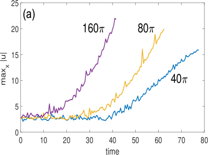
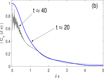
Figure 8: (a) Evolution of maximum amplitude of the field for three different lengths of the computational domain, listed in the figure.  (b) Magnitude of the spatial correlation function of the field for $L=160\pi$; see text for more details.

Second, if, hypothetically, the periodicity of the computational domain had played any constructive role in the pulse formation, then this formation would be impeded by increasing the domain’s length (since the longer the computational domain, the more it is similar to a true infinite domain). Therefore, to test this hypothesis, we repeated the simulation reported in Fig. 4, except that we used two longer computational domains: $L=80\pi$ and $L=160\pi$. The number of grid points was increased proportionally, so that the mesh size $\Delta x$ and hence the time step $\Delta t$ remained the same (see end of Appendix A).

In Fig. 8(a) we plot the maximum (over $x$) amplitude of the field for three different values of the domain length $L$. One can see that pulse formation is facilitated, rather than impeded, by an increased domain. This is manifested in both that the pulse forms sooner and that it reaches a greater amplitude in a longer domain. While a rigorous explanation of these facts is unknown to us, the following are plausible reasons behind them. First, an intense pulse begins to form out of some part of the field that already has an above-average amplitude. It seems likely that there are more locations with a stronger field in a longer domain, and hence the pulse can begin to form sooner. Second, the pulse can reach a greater amplitude in a longer domain because it has the opportunity to “harvest" energy from a larger “reservoir", which is the area where the field has about-average magnitude.

Finally, we return to our argument made after (33) that the correlation length of the field is much smaller than the domain length. To refute the possibility that the periodicity of the field (with period $L$) can affect pulse formation, it seems to make the most sense to compare $L$ with the field’s correlation length at a time when the formation commences. For the results shown in Fig. 8(a), these times are approximately 40, 30, and 20 for $L=40\pi$, $80\pi$, and $160\pi$, respectively. In Fig. 8(b) we show the correlation function (33) for $L=160\pi$ near $t=20$; for completeness we also show the same function near $t=40$, where the computation is terminated. The correlation functions for $L=40\pi$ and $80\pi$ look qualitatively similar and therefore are not shown. It is clear from Fig. 8(b) that the field become decorrelated over distances that are more than an order of magnitude smaller than the length of the computational domain.

Appendix C:  List of notations and acronyms used throughout the text

$\alpha=(+)$ or $(-)$:  labels positrons or electrons, respectively, in secondary plasma.

$B_{d}$:  dipolar component of magnetic field.

$B_{s}$:  magnetic field on surface of pulsar.

$b=B_{s}/B_{d}$.

$c$:  speed of light in vacuum.

$\Delta\gamma=|\gamma_{s,\,(+)}-\gamma_{s,\,(-)}|$:  difference between mean Lorentz factors of positrons and electrons in secondary plasma.

$\Delta R$:  distance along magnetic field lines where Langmuir turbulence is thought to be strong enough to lead to formation of coherent structures in charge density.

$\Delta V$:  potential drop across vacuum gap.

$E_{\|}$:  envelope of Langmuir wave.

$E_{0}$:  typical magnitude of $E_{\|}$ at a distance $R_{\rm onset}$.

$e$:  charge of electron ($e>0$).

$f_{\alpha}$:  momentum distribution function of type $\alpha$ particles in secondary plasma.

$\gamma_{b}\sim 2\times 10^{6}$: average Lorentz factor of primary plasma beam particles.

$\gamma_{p}\sim 10^{2}$: average Lorentz factor of electrons and positrons in secondary plasma;  $\gamma_{2}=\gamma_{p}/10^{2}$.

$\gamma_{\alpha},\,\gamma_{T}$:  mean and standard deviation of Lorentz factor $\gamma$ in the secondary plasma of type $\alpha$ particles.

$h\gtrsim 10^{3}$ cm:  height of the vacuum gap above the polar cap.

$G$:  group velocity dispersion coefficient in NLSE (13).

$G_{d}$:  related to $G$ by (14).

$\kappa=n_{p}/n_{b}\sim 10^{4}$;  $\kappa_{4}=\kappa/10^{4}$.

$\lambda_{l}$:  Langmuir wavelength in OFR.

$\lambda_{p}$:  Langmuir wavelength in MFR at some reference location (around $R\sim 50R_{s}$).

$L$:  nondimensional length of the computational domain used in section 6.

$l=c/\omega_{p}$:  characteristic scale of Lamgmuir waves in MFR, used for normalization in section 5.

$l_{\rm corr}$:  nondimensional correlation length of random field in initial condition (23a) for Langmuir wave.

$m_{e}$:  mass of electron.

MFR:  moving frame of reference.

$n_{G}J$:  Goldreich–Julian density.

$n_{b},\,n_{p}$:  density of electron-positron pairs in primary and secondary plasma, respectively.

NLSE:  nonlinear Schrödinger equation.

$\Omega=2\pi/P$:  angular frequency of pulsar (nondimensional).

$\omega_{l}\sim 4\times 10^{11}$ s^-1:  Langmuir frequency (in OFR).

$\omega_{p}\approx\omega_{l}/\gamma_{p}\sim 4\times 10^{9}$ s^-1:  Langmuir frequency (in MFR) at some reference location (around $R\sim 50R_{s}$).

OFR:  observer frame of reference.

$P\sim 1$:  period of pulsar rotation (in seconds).

$\dot{P}$:  rate of pulsar slow-down (nondimensional);  $\dot{P}_{-15}=\dot{P}/10^{-15}$.

$p_{\alpha},\,p_{T}$:  mean and standard deviation of the momentum distribution function $f_{\alpha}$ in the secondary plasma.

$q$:  dimensional nonlinearity coefficient in NLSE (13).

$q_{d}$:  related to $q$ by (15).

$Q$:  nondimensional nonlinearity coefficient in NLSE (20).

$\rho\sim 10^{6}$ cm:  curvature radius of magnetic field lines in the vacuum gap;  $\rho_{6}=\rho/(10^{6}\,{\rm cm})$.

$R_{s}$:  radius of pulsar (assumed to be 10 km in this paper).

$R$:  distance from pulsar;  $R_{50}=R/(50R_{s})\sim 1$.

$R_{em}$:  distance from the pulsar where coherent radio emission takes place.

$R_{\rm onset}\sim 200$ km:    distance from the pulsar where Langmuir turbulence is thought to begin to develop.

$r$:  relative part of random field in initial condition (23a) for Langmuir wave.

$s$:  coefficient of nonlinear Landau damping in NLSE (13).

$(s/q)$:  magnitude of nonlinear Landau damping relative to purely cubic nonlinearity in NLSE.

$s_{d}$:  related to $s$ by (16).

$\theta$:  ratio of the characteristic scales of the envelope and carrier of the Langmuir wave, defined after (17b);  $\theta\sim 10^{3}\ldots 10^{4}$.

$\tau,\,\tau_{\circ}$:  dimensional time variables in MFR and OFR, respectively; their relation is given after (13).

$t$:  nondimensional time in MFR, related to $\tau$ by (19).

$t_{4\times}$:  time that it takes amplitude of intense pulse to exceed four times average amplitude of initial state; see section 6.2.

$u$:  nondimensional envelope of Langmuir wave; see (18).

$\chi,\,\chi_{\circ}$:  dimensional spatial variables along magnetic field lines in MFR and OFR, respectively; their relation is given after (13).

$x$:  nondimensional space variable in MFR, related to $\chi$ by (17b).

References

- Agafontsev & Zakharov (2015) Agafontsev, D., & Zakharov, V. 2015, Nonlinearity, 28, 2791
- Arons & Scharlemann (1979) Arons, J., & Scharlemann, E. T. 1979, ApJ, 231, 854
- Asseo & Melikidze (1998) Asseo, E., & Melikidze, G. I. 1998, MNRAS, 301, 59
- Barman & Misra (2017) Barman, A., & Misra, A. 2017, Phys. Plasmas, 24, 052116
- Blasi & Amato (2011) Blasi, P., & Amato, E. 2011, Astrophysics and Space Science Proceedings, 21, 624
- Blaskiewicz et al. (1991) Blaskiewicz, M., Cordes, J. M., & Wasserman, I. 1991, ApJ, 370, 643
- Briggs et al. (1983) Briggs, W., Newell, A. C., & Sarie, T. 1983, J. Comp. Phys., 51, 83
- Chatterjee & Misra (2015) Chatterjee, D., & Misra, A. 2015, Phys. Rev. E, 92, 063110
- Chaudhuri & Roy Chowdhury (2018) Chaudhuri, S., & Roy Chowdhury, A. 2018, Phys. Scr., 93, 075601
- Cheng & Ruderman (1979) Cheng, A. F., & Ruderman, M. A. 1979, ApJ, 229, 348
- Contopoulos et al. (1999) Contopoulos, I., Kazanas, D., & Fendt, C. 1999, ApJ, 511, 351
- Dyks (2008) Dyks, J. 2008, MNRAS, 391, 859
- Dyks et al. (2004) Dyks, J., Rudak, B., & Harding, A. K. 2004, ApJ, 607, 939
- Ehsan et al. (2009) Ehsan, Z., Tsintsadze, N., Vranjes, J., & Poedts, S. 2009, Phys. Plasmas, 16, 053702
- Everett & Weisberg (2001) Everett, J. E., & Weisberg, J. M. 2001, ApJ, 553, 341
- Fedele et al. (2010) Fedele, F., Cherneva, Z., Tayfun, M. A., & Guedes Soares, C. 2010, Phys. Fluids, 22, 036601
- Flå et al. (1989) Flå, T., Mjølhus, E., & Wyller, J. 1989, Phys. Scr., 40, 219
- Gelash & Agafontsev (2018) Gelash, A., & Agafontsev, D. 2018, arXiv:1804.00652v3
- Genty et al. (2010) Genty, G., de Sterke, C. M., Bang, O., et al. 2010, Phys. Lett. A, 374, 989
- Geppert (2017) Geppert, U. 2017, Journal of Astrophysics and Astronomy, 38, 46
- Gil et al. (2004) Gil, J., Lyubarsky, Y., & Melikidze, G. I. 2004, ApJ, 600, 872
- Gil & Mitra (2001) Gil, J., & Mitra, D. 2001, ApJ, 550, 383
- Ginzburg & Zhelezniakov (1975) Ginzburg, V. L., & Zhelezniakov, V. V. 1975, ARA&A, 13, 511
- Goldreich & Julian (1969) Goldreich, P., & Julian, W. H. 1969, ApJ, 157, 869
- Ichikawa & Tanuiti (1973) Ichikawa, Y., & Tanuiti, T. 1973, J. Phys. Soc. Japan, 34, 513
- Johnson et al. (2012) Johnson, M. D., Gwinn, C. R., & Demorest, P. 2012, ApJ, 758, 8
- Johnston et al. (2005) Johnston, S., Hobbs, G., Vigeland, S., et al. 2005, MNRAS, 364, 1397
- Jordan & Josserand (2001) Jordan, R., & Josserand, C. 2001, Math. Comp. Simul., 55, 443
- Kalapotharakos & Contopoulos (2009) Kalapotharakos, C., & Contopoulos, I. 2009, A&A, 496, 495
- Kazbegi et al. (1991) Kazbegi, A. Z., Machabeli, G. Z., & Melikidze, G. I. 1991, MNRAS, 253, 377
- Lai et al. (2001) Lai, D., Chernoff, D. F., & Cordes, J. M. 2001, ApJ, 549, 1111
- Lakoba (2015) Lakoba, T. I. 2015, Phys. Lett. A, 379, 1821
- Lakoba (2016) —. 2016, J. Sci. Comp., 72, 14
- Lominadze et al. (1986) Lominadze, D. G., Machabeli, G. Z., Melikidze, G. I., & Pataraia, A. D. 1986, Soviet J. Plasma Phys., 12, 712
- Meiss & Morrison (1983) Meiss, J., & Morrison, P. 1983, Phys. Fluids, 26, 983
- Melikidze et al. (2000) Melikidze, G. I., Gil, J. A., & Pataraya, A. D. 2000, ApJ, 544, 1081
- Melikidze et al. (2014) Melikidze, G. I., Mitra, D., & Gil, J. 2014, ApJ, 794, 105
- Melikidze & Pataraya (1980) Melikidze, G. I., & Pataraya, A. D. 1980, Astrophysics, 16, 104
- Melikidze & Pataraya (1984) —. 1984, Astrophysics, 20, 100
- Misra & Barman (2015) Misra, A., & Barman, A. 2015, Phys. Plasmas, 22, 073708
- Misra et al. (2017) Misra, A., Chatterjee, D., & Brodin, G. 2017, Phys. Rev. E, 96, 053209
- Mitra (2017) Mitra, D. 2017, Journal of Astrophysics and Astronomy, 38, 52
- Mitra et al. (2009) Mitra, D., Gil, J., & Melikidze, G. I. 2009, ApJ, 696, L141
- Mitra & Li (2004) Mitra, D., & Li, X. H. 2004, A&A, 421, 215
- Mitra et al. (2016) Mitra, D., Rankin, J., & Arjunwadkar, M. 2016, MNRAS, 460, 3063
- Mitra & Rankin (2011) Mitra, D., & Rankin, J. M. 2011, ApJ, 727, 92
- Pataraia & Melikidze (1980) Pataraia, A., & Melikidze, G. 1980, Ap&SS, 68, 61
- Pétri (2016) Pétri, J. 2016, J. Plasma Phys., 82, 635820502
- Radhakrishnan & Cooke (1969) Radhakrishnan, V., & Cooke, D. J. 1969, Astrophys. Lett., 3, 225
- Rankin (2007) Rankin, J. M. 2007, ApJ, 664, 443
- Roy Chowdhury et al. (1988) Roy Chowdhury, A., Pakira, G., & Paul, S. 1988, Phys. C, 151, 518
- Ruderman & Sutherland (1975) Ruderman, M. A., & Sutherland, P. G. 1975, ApJ, 196, 51
- Sloan & Mitchell (1986) Sloan, D. M., & Mitchell, A. R. 1986, J. Comp. Phys., 67, 372–395
- Solli et al. (2007) Solli, D. R., Ropers, C., Koonath, P., & Jalali, B. 2007, Nature, 450, 1054
- Spitkovsky (2006) Spitkovsky, A. 2006, ApJ, 648, L51
- Spitkovsky (2011) —. 2011, Astrophysics and Space Science Proceedings, 21, 139
- Sturrock (1971a) Sturrock, P. A. 1971a, ApJ, 164, 529
- Sturrock (1971b) —. 1971b, ApJ, 164, 529
- Timokhin (2006) Timokhin, A. N. 2006, MNRAS, 368, 1055
- Timokhin (2010) —. 2010, MNRAS, 408, 2092
- Timokhin & Arons (2013) Timokhin, A. N., & Arons, J. 2013, MNRAS, 429, 20
- Timokhin & Harding (2015) Timokhin, A. N., & Harding, A. K. 2015, ApJ, 810, 144
- Usov (1987) Usov, V. V. 1987, ApJ, 320, 333
- von Hoensbroech & Xilouris (1997) von Hoensbroech, A., & Xilouris, K. M. 1997, A&A, 324, 981
- Weiland et al. (1978) Weiland, J., Ichikawa, Y., & Wilhelmsson, H. 1978, Phys. Scr., 17, 517
- Weltevrede & Johnston (2008) Weltevrede, P., & Johnston, S. 2008, MNRAS, 391, 1210
- Young et al. (1999) Young, M. D., Manchester, R. N., & Johnston, S. 1999, Nature, 400, 848