Linked and knotted synthetic magnetic fields

Abstract

We show that the realisation of synthetic magnetic fields via light-matter coupling in the $\Lambda$-scheme implements a natural geometrical construction of magnetic fields, namely as the pullback of the area element of the sphere to Euclidean space via certain maps. For suitable maps, this construction generates linked and knotted magnetic fields, and the synthetic realisation amounts to the identification of the map with the ratio of two Rabi frequencies which represent the coupling of the internal energy levels of an ultracold atom. We consider examples of maps which can be physically realised in terms of Rabi frequencies and which lead to linked and knotted synthetic magnetic fields acting on the neutral atomic gas. We also show that the ground state of the Bose-Einstein condensate may inherit topological properties of the synthetic gauge field, with linked and knotted vortex lines appearing in some cases.

I Introduction

Lord Kelvin’s conjecture 150 years ago that atoms are made of knotted vortex structures Thomson (1867) anticipated today’s study, both theoretical and experimental, of topological structures in nature. Non-trivial topological structures have been studied in classical fluids Moffatt (1969); Moffatt and Tsinober (1992); Kleckner and Irvine (2013); Enciso and Peralta-Salas (2013); Scheeler et al. (2014), plasma physics Chandrasekhar and Woltjer (1958); Berger (1999); Thompson et al. (2014), nuclear physics Battye and Sutcliffe (1998); Sutcliffe (2007), condensed matter physics Sutcliffe (2017), DNA Taylor (2000); Suma and Micheletti (2017), soft matter Tkalec et al. (2011) and light Irvine and Bouwmeester (2008); Irvine (2010); Kedia et al. (2013, 2018). There has also been interest in the physics of topological magnetic field lines, with research focusing on their construction Kedia et al. (2016) and stability Kleckner and Irvine (2013); Scheeler et al. (2014); Kleckner et al. (2016). Understanding the behaviour of matter in non-trivial topological magnetic fields is also important in the study of plasma physics and the determination of stable confining magnetic field configurations in thermonuclear reactors Moffatt (2014, 2015).

Ultracold atoms allow the realisation of synthetic gauge fields in such a way that neutral atoms mimic the dynamics of charged particles in a magnetic field Lin et al. (2009a, b, 2011); Zhu et al. (2006); Dalibard et al. (2011); Goldman et al. (2014). One method of creating a synthetic gauge field is to exploit atom-light couplings by driving internal transitions of the atoms to realize static Abelian gauge fields which are tunable via the applied laser Juzeliūnas and Öhberg (2004); Juzeliūnas et al. (2005, 2006). There has also been significant interest in creating knotted structures in quantum gases Liang et al. (2009); Liu and Yang (2013); Liu et al. (2014); Proment et al. (2014); Bidasyuk et al. (2015), with the first knots in quantum matter having been realised in spinor BECs Kawaguchi et al. (2008); Hall et al. (2016). Further experiments have investigated the formation of a Shankar skyrmion in the spinor BECs with knotted spin structure Shankar (1977); Lee et al. (2018). The imprinting of linked and knotted vortex structures has also been proposed using driving schemes of the internal energy levels Ruostekoski and Dutton (2005); Maucher et al. (2016).

The formation of knotted vortex lines (or knotted solitons) has been extensively investigated in superfluids and superconductors Babaev et al. (2002); Babaev (2002, 2004), including the conditions for their stability in multicomponent superconductors Rybakov et al. (2018). In addition, there have been proposals for fault-tolerant Shor (1995) topologically protected quantum computations Kitaev (2003); Nayak et al. (2008) using vortices in superconductors Read and Green (2000); Das Sarma et al. (2006) and spin interactions in optical lattices Jaksch et al. (1999); Duan et al. (2003). The knotted vortices considered in superconductors are of a different nature from those we consider here. However, as we will explain in Sec. V, that knotted or linked magnetic fields generically open up new avenues for quantum computing.

In this paper, we point out and exploit a remarkably direct link between the realisation of synthetic magnetic fields in ultracold atoms and a mathematical construction of knotted and linked magnetic fields, due to Rañada Rañada (1989); Ranada (1990), out of a map from Euclidean 3-space to the 2-sphere. In a nutshell, we show that this map can be realised as the ratio of two complex Rabi frequencies describing the atom-light coupling in a three-level atomic $\Lambda$-scheme.

The mathematically most natural choice of the Rañada map for a given link or knot is challenging to implement directly in an experiment, but our results suggest that one can implement an approximation to this map which, crucially, preserves the topology of the knot or link. We propose a general method for constructing this approximation, and illustrate it with three examples of maps, called $f_{H},f_{L}$ and $f_{T}$, whose associated magnetic field lines are, respectively, Hopf circles, linked rings and the trefoil knot.

Finally, we find that some of the topological structure of the synthetic gauge field lines is inherited by the ground state of the dark-state wavefuntion in the $\Lambda$-scheme. The details of this depend on the potential and magnetic field which appear in the effective Hamiltonian. For instance, if the scalar potential is peaked along a knot or link, the wavefunction reflects this through a vortex structure along that knot or link. This happens for the trefoil knot and linked rings, but not for the Hopf circles, where the scalar potential is spherically symmetric. A similar interplay between linked magnetic field lines and vortex lines in a spinorial wavefunction was recently studied in Ref. Ross and Schroers (2018).

II Rañada’s knotted light

In the 1980s, Rañada proposed a systematic mathematical construction of linked or knotted electric and magnetic fields Rañada (1989); Ranada (1990). This construction has a beautiful geometrical interpretation in terms of the geometry of the 2-sphere which we review briefly in Appendix A. It leads to an explicit formula for a magnetic field in terms of a map $f:\mathbb{R}^{3}\rightarrow S^{2}$. Identifying the 2-sphere with $\mathbb{C}\cup\{\infty\}$ via the stereographic projection, the magnetic field is

$$\mathbf{B}=\frac{1}{2\pi i}\frac{\nabla f^{*}\times\nabla f}{\left(1+\lvert f\rvert^{2}\right)^{2}}.$$ (1)

This field has vanishing divergence, and therefore satisfies the static Maxwell equations, generally with a non-trivial current. Moreover, one checks that field lines are determined by the (complex) condition $f=$ constant. In this way one can therefore construct topologically interesting magnetic fields by drawing on the extensive mathematical literature studying links and knots as level curves of complex functions. The formulation of the magnetic field in Eq. (1), along with the definition of the maps, has been utilised to study the properties of topologically non-trivial vector fields Irvine and Bouwmeester (2008); Besieris and Shaarawi (2009); Kedia et al. (2013); Thompson et al. (2014); Kedia et al. (2016, 2018).

The maps $\mathbb{R}^{3}\rightarrow S^{2}$ considered by Rañada and in this paper go via $S^{3}$, i.e. they are compositions

$$f:\mathbb{R}^{3}\rightarrow S^{3}\rightarrow S^{3}\rightarrow S^{2},$$ (2)

where the first step is the inverse stereographic projection in three dimensions, and the last step is projection of the Hopf fibration. The details of the map are encoded in the intermediate step $S^{3}\rightarrow S^{3}$. Using complex coordinates $u,v\in\mathbb{C}$ satisfying $\lvert u\rvert^{2}+\lvert v\rvert^{2}=\mathit{l}^{2}$ to parametrise the 3-sphere of radius $\mathit{l}$, the inverse stereographic projection maps $(x,y,z)\in\mathbb{R}^{3}$ to

$$u=\frac{2\mathit{l}^{2}\left(x+iy\right)}{\mathit{l}^{2}+r^{2}},\>\>v=\frac{2\mathit{l}^{2}z+i\mathit{l}\left(r^{2}-\mathit{l}^{2}\right)}{\mathit{l}^{2}+r^{2}},$$ (3)

with $r^{2}=x^{2}+y^{2}+z^{2}$ and $\mathit{l}$ setting the unit of length. The map (2) then takes the form

$$f\left(x,y,z\right)=\frac{g\left(u\left(x,y,z\right),v\left(x,y,z\right)\right)}{h\left(u\left(x,y,z\right),v\left(x,y,z\right)\right)},$$ (4)

where $g$ and $h$ are complex functions of $u$, $v$ which must not vanish simultaneously.

In this paper we focus on three examples; the standard Hopf map $f_{H}=u/v$ (defining Hopf circles), the quadratic Hopf map $f_{L}=u^{2}/(u^{2}-v^{2})$ (defining linked rings) and the map $f_{T}=u^{3}/(u^{3}+v^{2})$ which defines the trefoil knot. The first two define links whose topology is independent of the chosen (complex) level; the level curves of $f_{H}$ are circles or the $z$-axis (an “infinite circle”), and any two circles link once. The level curves of $f_{L}$ are linked rings or the $z$-axis; different level curves link each other four times. The third map defines a trefoil knot for level $\infty$ or sufficiently large.

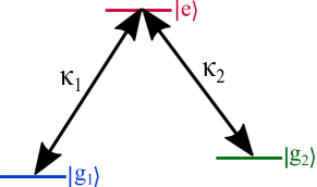
Figure 1: Illustration of the $\Lambda$-scheme, with internal atomic energy levels $|{e}\rangle$, $|{g_{1}}\rangle$ and $|{g_{2}}\rangle$ coupled by lasers $\kappa_{1}$ and $\kappa_{2}$.

III The $\Lambda$-scheme

Synthetic gauge potentials for ultracold atoms can be realised in many ways Dalibard et al. (2011); Goldman et al. (2014). We consider an ensemble of atoms with three internal energy levels where two ground states $|g_{1}\rangle$ and $|g_{2}\rangle$ are coupled by two laser beams to a third excited state $|{e}\rangle$. This configuration of energy levels is called a $\Lambda$-scheme, and is illustrated in Fig. 1. The strength of the atom-light coupling is characterised through space-dependent, complex Rabi frequencies $\kappa_{1},\kappa_{2}$. We assume the lasers are resonant with the transitions, and with zero two-photon detuning, resulting in the atom-light coupling Hamiltonian

$$H_{\mathrm{int}}=\left(\begin{matrix}0&0&\kappa_{1}\\ 0&0&\kappa_{2}\\ \kappa_{1}^{*}&\kappa_{2}^{*}&0\end{matrix}\right).$$ (5)

A general state of the light-matter coupled system can then be written as $|\Psi\rangle=\sum_{i=D,+,-}\psi_{i}(x)|i\rangle$ where $|D\rangle,|+\rangle,|-\rangle$ depend parametrically on space and are the three eigenstates of $H_{\mathrm{int}}$. The eigenstate for eigenvalue zero is the dark state

$$|{D}\rangle=\frac{1}{\sqrt{|\kappa_{1}|^{2}+|\kappa_{2}|^{2}}}\begin{pmatrix}\phantom{-}\kappa_{2}^{*}\\ -\kappa_{1}^{*}\\ \phantom{-}0\end{pmatrix}.$$ (6)

It has no contribution from the excited state and is therefore also robust against detrimental spontaneous decay.

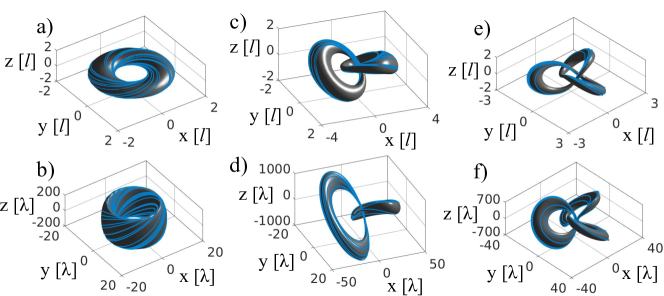
Figure 2: Exact and approximated magnetic field lines, realised as level curves of the complex field $f$ and its Laguerre-Gauss approximation $\zeta$ . We show level surfaces of $|f|$ and $|\zeta|$, and, on each level surface, we show magnetic field lines in light blue. a) Exact Hopf circles ($f_{H}$). b) Realised Hopf circles ($\zeta_{H}$). c) Exact linked rings ($f_{L}$). d) Realised linked rings ($\zeta_{L}$). e) Exact trefoil knot ($f_{T}$). f) Realised trefoil knot ($\zeta_{T}$). The unit of length for the exact magnetic fields is $l$ and for the realised fields it is the laser wavelength $\lambda$ with $\alpha=100$.

If we include the kinetic term and a confining potential $V$ in the full Hamiltonian $H=\frac{\mathbf{p}^{2}}{2m}+H_{\mathrm{int}}+V$ and, using the adiabatic approximation, project the corresponding Schrödinger equation $i\hbar\partial_{t}|\Psi\rangle=H|\Psi\rangle$ onto the dark state while neglecting the coupling to the other dressed states, then $\psi_{D}$ is governed by the equation of motion

$$i\hbar\frac{\partial}{\partial t}\psi_{D}=\left[\frac{\left(\mathbf{p}-\mathcal{A}\right)^{2}}{2m}+\Phi+V\right]\psi_{D}.$$ (7)

The vector potential $\mathcal{A}$, the corresponding magnetic field $\mathcal{B}$ and geometric potential $\Phi$ are fully determined by the Rabi coefficients $\kappa_{1},\kappa_{2}$, with the magnetic field and scalar potential conveniently expressed in terms of $\zeta=\kappa_{1}/\kappa_{2}$. Explicitly we have

$$\mathcal{A}=\frac{i\hbar(\kappa_{1}\nabla\kappa^{*}_{1}+\kappa_{2}\nabla\kappa^{*}_{2}-\kappa^{*}_{1}\nabla\kappa_{1}-\kappa^{*}_{2}\nabla\kappa_{2})}{2(|\kappa_{1}|^{2}+|\kappa_{2}|^{2})},$$ (8)

$$\mathcal{B}=i\hbar\frac{\nabla\zeta\times\nabla\zeta^{*}}{\left(1+\lvert\zeta\rvert^{2}\right)^{2}},$$ (9)

$$\Phi=\frac{\hbar^{2}}{2m}\frac{\nabla\zeta^{*}\cdot\nabla\zeta}{\left(1+\lvert\zeta\rvert^{2}\right)^{2}}.$$ (10)

Note, that expressing $\mathcal{A}$ in terms of $\zeta$ would lead to a singular gauge.

For the synthetic magnetic field and its corresponding gauge potential to be experimentally viable, the life-time of the dark state needs to be long enough. For example, spontaneous emissions from the excited state would change the life time of the dark state, but this is mitigated if the Rabi frequency is large enough to ensure the adiabatic approximation is valid. In addition, strong collisional interactions should be avoided, as any atom-atom interactions will be detrimental to the stability of the dark state. This can be addressed by ensuring the atoms are in the dilute limit or the scattering length is tuned to be small. We also require that any Zeeman coupling terms between the two ground states of the $\Lambda$-scheme are sufficiently small to allow them to be neglected.

If we identify $\zeta\equiv f$ then the magnetic fields of Rañada, Eq. (1), and the $\Lambda$-scheme, Eq. (9), are equivalent (in fact, equal with $\hbar=1/2\pi$). Therefore, to realize the topological magnetic field of a particular $f$ we are required to drive the atomic transitions by the Rabi frequencies such that their ratio, $\zeta$, forms the mapping $f$. The Rabi frequencies $\kappa_{1}$ and $\kappa_{2}$ can be chosen independently, giving a considerable amount of flexibility and allowing us, in principle, to realise any link or knot which is the level curve of a function $f:\mathbb{R}\rightarrow S^{2}$. However, we can not set the Rabi frequencies to be any arbitrary function of space and phase, as they are realised by laser beams which need to fulfil Maxwell’s equations. This restriction on the allowed forms of the Rabi frequencies is at the heart of our discussion in the next section.

IV Realisation of topological fields.

Our approach is inspired by Refs. Dennis et al. (2010); Romero et al. (2011); Padgett et al. (2011), where linked and knotted optical vortex lines were realised in laser beams as a superposition of Laguerre-Gaussian (LG) modes. These superpositions of LG modes are usually obtained by the use of Spatial Light Modulators (SLMs) McGloin et al. (2003); Bergamini et al. (2004); Boyer et al. (2006); Olson et al. (2007); Gaunt et al. (2013); Nogrette et al. (2014); van Bijnen et al. (2015). LG beams are characterised by their azimuthal, $n$, and radial, $p$, indices, and we will denote a single LG mode as $\mathcal{L}_{pn}$, with the full definition of a LG mode discussed in Appendix B. Our method of constructing the topological synthetic magnetic fields consists of the following steps:

1. Starting from a map $f$ of the form (4), restrict it to the $z=0$ plane, where $z$ is the direction of propagation for the lasers, and note that the result is a ratio of polynomials $p$ and $q$ in $x$ and $y$.

2. Expand the polynomials $p$ and $q$ in terms of LG modes restricted to the $z=0$ plane and without the common Gaussian factor.

3. Replace $p$ and $q$ in $f$ by the expansions in the LG modes, including their $z$-dependence (and note that the common Gaussian factor cancels).

4. Check numerically if the level curves of the resulting function $\zeta$ have the same topology as the level curves of $f$.

5. If they do, realise the level curves as synthetic magnetic field lines via $\zeta=\kappa_{1}/\kappa_{2}$, where $\kappa_{1}$ and $\kappa_{2}$ are the LG modes approximating $g$ and $h$.

All three examples considered in this work pass the check in step 4, but we are not aware of a mathematical proof that this should be true generally.

IV.1 Form of the topological magnetic fields

Expanding in terms of LG modes we find the following approximations for the Hopf map $f_{H}$, the quadratic Hopf map $f_{L}$ and the map $f_{T}$ for the trefoil knot:

$$\zeta_{H}=\frac{2\alpha\mathcal{L}_{0-1}}{i\left[\left(\frac{\alpha^{2}}{2}-1\right)\mathcal{L}_{00}-\frac{\alpha^{2}}{2}\mathcal{L}_{10}\right]},$$ (11)

$$\zeta_{L}=\frac{(2\alpha)^{2}\mathcal{L}_{0-2}}{(2\alpha)^{2}\mathcal{L}_{0-2}+c_{0}\mathcal{L}_{00}+c_{1}\mathcal{L}_{10}+c_{2}\mathcal{L}_{20}},$$ (12)

$$\zeta_{T}=\frac{(2\alpha)^{3}\mathcal{L}_{0-3}}{(2\alpha)^{3}\mathcal{L}_{0-3}+c^{\prime}_{0}\mathcal{L}_{00}+c^{\prime}_{1}\mathcal{L}_{10}+c^{\prime}_{2}\mathcal{L}_{20}+c^{\prime}_{3}\mathcal{L}_{30}},$$ (13)

where we have defined $\alpha=\omega_{0}/l$ with $\omega_{0}$ the beam waist of the laser. Definitions of the coefficients $c_{i}$ and $c^{\prime}_{i}$, which are polynomials in $\alpha$, can be found in Appendix B.

A comparison of the exact and realised magnetic fields for all three cases considered is shown in Fig. 2. For all realised fields we have chosen a beam width of $\alpha=100$ and work in units of the wavelength of the laser $\lambda$. The realised fields are found to be stretched out in the $z$-direction compared to the exact fields. For all three examples considered the topological nature of the realised magnetic field lines is clear, as the level set of each have similar forms to that of the exact fields.

IV.2 Beam shaping realisation

We note here that the specific combinations of LG modes discussed in the previous subsection is entirely a beam shaping excercise. That is, the superposition of the LG modes in the denominators of Eqs. (11-13) results in a single beam with the required intensity and phase profiles. This single beam is then used as $\kappa_{2}$ in the driving of the $\Lambda$-scheme.

The atomic transitions accessed in a $\Lambda$-scheme are typically in the optical regime and thus the diffraction limit of $0.2~{}\mu m-~{}0.4~{}\mu m$ sets the length scale limit. Furthermore, the resolution of current beam shaping technology imposes limits on the spatial resolution of the resulting gauge field and on the field strength. The atomic cloud size ($\sim 100\mu m$ Jaouadi et al. (2010)) is typically smaller than the usual beam waists considered (e.g. $\sim 1mm$ Leach et al. (2005)). Nonetheless, we do not foresee that the gauge field configurations discussed here will fall outside what is currently experimentally achievable, as it is not unusual to focus optical beams down to beam waists of $50-200\mu m$ in other settings Roger et al. (2016); Caspani et al. (2016).

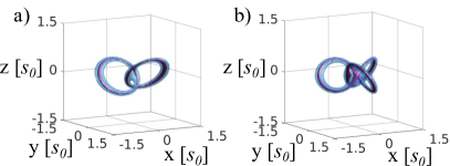
Figure 3: Vortex structure of the ground states of the Hamiltonian in (7) with a vector potential constructed from a) $f_{L}$ and b) $f_{T}$. Shown are level sets of the probability density ($|\psi|^{2}=\mathrm{const.}$) for a small constant, which visualises the vortex core structure. The vortices form linked rings in a) and a trefoil knot in b), thus replicating the form of the magnetic field lines in both cases.

IV.3 Ground state of the quantum gas

In order to illustrate the effect the knotted synthetic magnetic fields can have on atoms, we envisage a non-interacting gas of atoms forming a three-dimensional Bose-Einstein condensate which is trapped by a harmonic external potential $V=m\omega^{2}r^{2}/2$, where $\omega$ is the trap frequency. We are interested in the properties of the ground state of such a condensate which is interacting with a linked or knotted magnetic field and a geometric potential via Eq. (7). We solve for the ground state $\psi=\psi_{\mathrm{D}}$ using imaginary time propagation Chiofalo et al. (2000); Roy et al. (2001); Bader et al. (2013) on a $201^{3}$ numerical grid and for the three exact gauge fields defined via the maps $f_{\mathrm{H}}$, $f_{\mathrm{L}}$ and $f_{\mathrm{T}}$. We choose our unit of length to be $s_{0}=\sqrt{\hbar/m\omega}$ and take $l=1$. It is not immediately obvious what the properties of the ground states of this system should be. The ground state is dependent on the interplay between the strength and shape of the topologically non-trivial magnetic field, the corresponding scalar potential, and the trapping potential. The ground states discussed here reflect the choice of considering a cloud of cold atoms confined in a harmonic potential.

We observe the presence of vortex structures in the ground states for the linked rings and the trefoil knot, which are shown in Fig. 3 by the level sets of $|\psi|^{2}$ and in the supplemental movies Sup . However, there is no vortex structure in the ground state for the Hopf circles shown in Fig. 4, for this choice of parameters. The vortex structures in the other ground states are determined by the maxima of the scalar potential $\Phi$, whose level sets for near-maximal values are very similar to the level sets for small probability density shown in Fig. 3. We are not aware of a simple mathematical reason for the relation between the level sets of $\Phi$ and the magnetic field lines which we observe for the linked rings and the trefoil knot.

The detection of such topological structures in the gas requires a tomographic approach where 3D vortex core structure are imaged using a non-destructive measurement of the density Higbie et al. (2005). Alternatively, the presence of non-trivial gauge fields can be indirectly detected by measuring the shape oscillations of the gas Murray et al. (2007).

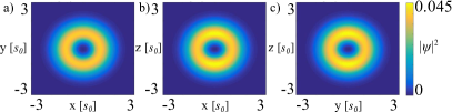
Figure 4: Ground state of the Hamiltonian in (7) with a vector potential constructed from $f_{H}$. The probability density is shown in the a) $xy$-plane ($z=0$), b) $xz$-plane ($y=0$) and c) $yz$-plane ($x=0$). The ground state is real valued and forms a shell structure which is close to spherical but slightly elongated in the $z$-direction. Note that the geometric potential $\Phi$ is spherically symmetric in this case, but the magnetic field is not

V Conclusions

We have shown that certain magnetic fields which are the pullback of the normal area element of the 2-sphere to Euclidean 3-space can be realised as a synthetic magnetic field in the resonant $\Lambda$-scheme. Based on this observation, we propose a five-step method of realising general synthetic topological magnetic fields using a superposition of LG modes. We have derived the required LG superpositions for three examples – the Hopf circles, the linked rings and the trefoil knot – and shown their topological nature. In some cases, the topological form of these magnetic fields can be transferred to the ground states of the ultracold gas in the form of linked and knotted vortex cores. The general method presented in this work is not limited to the three examples considered, and we expect more links and knots defined by a map $f$ to be realisable.

The 3D-nature of the generated states and the versatility of our method opens a possible avenue for a physical realisation of the motion group of links or knots Goldsmith (1981); Aneziris et al. (1991). This group is a generalisation of the braid group of a surface, and includes elements which describe truly three-dimensional motions, for example motions where one circle is pulled through another. If such motions proceed through configurations which are the level sets of a complex-valued function they can, in principle, be realised in our scheme. The quantum states of the condensate would potentially pick up exotic and non-abelian phases in such motions, reflecting the intricate (and little studied) representation theory of the motion group. It would clearly be interesting to investigate this possibility and to study its potential use in fault-tolerant topologically protected quantum computing.

Appendix A Differential geometry behind Rañada’s construction

Rañada’s construction of a magnetic field in terms of a map $f:\mathbb{R}^{3}\rightarrow S^{2}$ is most easily stated in the language of differential forms and pull-backs. This clarifies the coordinate-independent nature of the formula for the magnetic field, and provides a basis for generalisations. We give a succinct summary here, referring the reader to textbooks like Fecko (2006) for the differential-geometric background.

A fundamental role is played by the 2-form representing the area element $\Omega$ of the 2-sphere. Parametrising the 2-sphere via stereographic projection in terms of a complex coordinate $\mathcal{Z}\in\mathbb{C}\cup\{\infty\}$, this 2-form is

$$\Omega=\frac{1}{2\pi i}\frac{d\mathcal{Z}^{*}\wedge d\mathcal{Z}}{\left(1+\lvert\mathcal{Z}\rvert^{2}\right)^{2}}.$$ (14)

It is manifestly closed, i.e. satisfies $d\Omega=0$, and normalised to unit area. Given a map $f:\mathbb{R}^{3}\rightarrow S^{2}$, Rañada’s magnetic field is the pull-back

$$f^{*}\Omega=\frac{1}{2\pi i}\frac{df^{*}\wedge df}{\left(1+\lvert f\rvert^{2}\right)^{2}}$$ (15)

of $\Omega$ with $f$. This pull-back is a 2-form on $\mathbb{R}^{3}$ and automatically closed: it satisfies $d(f^{*}\Omega)=0$ because pull-back commutes with the exterior derivative. The magnetic field $\mathbf{B}$ given by Eq. (1) in the main text is the vector field associated to $f^{*}\Omega$ using the metric and volume element of Euclidean space. The closure of $f^{*}\Omega$ is then equivalent to $\mathbf{B}$ having vanishing divergence.

Appendix B Laguerre-Gaussian expansion technique

We provide the details for the expansions of the three example maps

$$f_{H}=\frac{u}{v},\quad f_{L}=\frac{u^{2}}{u^{2}-v^{2}},\quad f_{T}=\frac{u^{3}}{u^{3}+v^{2}},$$ (16)

considered in the main text in terms of the complete set of Laguerre-Gaussian (LG) beams, following the five-step method also proposed in the main text. The LG modes are

$$\mathcal{L}_{pn}\left(\rho,\phi,z\right)=\frac{C}{\sqrt{1+\frac{z^{2}}{z_{R}^{2}}}}\left(\frac{\rho\sqrt{2}}{w\left(z\right)}\right)^{|n|}L^{|n|}_{p}\left(\frac{2\rho^{2}}{w^{2}\left(z\right)}\right)e^{-\frac{\rho^{2}}{w^{2}\left(z\right)}}e^{-\frac{ik\rho^{2}z}{2\left(z^{2}+z_{R}^{2}\right)}}e^{-in\phi}e^{i\left(2p+|n|+1\right)\arctan\frac{z}{z_{R}}},$$ (17)

with $(\rho,\phi,z)$ being the cylindrical coordinates, $n$ the azimuthal index giving the angular momentum, $p$ the radial index and $C$ a normalisation constant. We use the usual optical definitions of the beam waist $w(z)=\omega_{0}\sqrt{1+(z/z_{R})^{2}}$ and Rayleigh range $z_{R}=\pi\omega_{0}^{2}/\lambda$. For $z=0$, the LG modes can be written as

$$\mathcal{L}_{pn}\left(\rho,\phi,0\right)=\frac{\tilde{C}}{w_{0}}e^{-\frac{\rho^{2}}{w_{0}^{2}}}L^{n}_{p}\left(\frac{2\rho^{2}}{w_{0}^{2}}\right)\left(\frac{x-iy}{w_{0}}\right)^{n}.$$ (18)

The functions $f_{H},f_{L}$ and $f_{T}$ are ratios of polynomials $g$ and $h$ in the complex coordinates $u$ and $v$, which, in turn, are functions of the Cartesian coordinates $(x,y,z)$ as given in the main text. Restricting $f_{H},f_{L}$ and $f_{T}$ to $z=0$, we obtain ratios of polynomials $p$ and $q$ in the variables $x$ and $y$. Expanding in LG modes without the overall Gaussian factor $\exp(-\rho^{2}/{w_{0}^{2}})$ we obtain an expansions with coefficients which are polynomials in the parameter $\alpha\equiv\omega_{0}/l$.

In this way, we arrive at the following exact identities:

$$\left.f_{H}\right|_{z=0} =\left.\frac{2\alpha\mathcal{L}_{0-1}}{i\left[\left(\frac{\alpha^{2}}{2}-1\right)\mathcal{L}_{00}-\frac{\alpha^{2}}{2}\mathcal{L}_{10}\right]}\right|_{z=0},$$

$$\left.f_{L}\right|_{z=0} =\left.\frac{(2\alpha)^{2}\mathcal{L}_{0-2}}{(2\alpha)^{2}\mathcal{L}_{0-2}-\left(-\frac{\alpha^{4}}{2}+\alpha^{2}-1\right)\mathcal{L}_{00}-\left(\alpha^{4}-\alpha^{2}\right)\mathcal{L}_{10}+\frac{\alpha^{4}}{2}\mathcal{L}_{20}}\right|_{z=0},$$

$$\left.f_{T}\right|_{z=0} =\left.\frac{(2\alpha)^{3}\mathcal{L}_{0-3}}{(2\alpha)^{3}\mathcal{L}_{0-3}+\frac{1}{4}\left[\left(-4+2\alpha^{2}+2\alpha^{4}-3\alpha^{6}\right)\mathcal{L}_{00}+\alpha^{2}\left(-2-4\alpha^{2}+9\alpha^{4}\right)\mathcal{L}_{10}+\left(2\alpha^{4}-9\alpha^{6}\right)\mathcal{L}_{20}+3\alpha^{6}\mathcal{L}_{30}\right]}\right|_{z=0}.$$

Dropping the restriction on the expressions on the right-hand-side to $z=0$ defines the approximations $\zeta_{H},\zeta_{L}$ and $\zeta_{T}$ to the functions $f_{H},f_{L}$ and $f_{T}$ which we used in the main text. The coefficients $c_{i}$ and $c_{i}^{\prime}$ used there are defined by the above expansions.

As discussed in the main text, the $\Lambda$-configuration synthetic magnetic fields are obtained using two laser beams with Rabi frequencies $\kappa_{1}$ and $\kappa_{2}$ given by the numerator and denominator of $\zeta_{H},\zeta_{L}$ and $\zeta_{T}$. In all cases, $\zeta=\kappa_{1}/\kappa_{2}$ provides a physically realisable approximation to the given function $f$ and yields synthetic magnetic field lines whose topology agrees with that of the level curves of the complex function $f$.

References

- Thomson (1867) W. Thomson, Philosophical Mag. 34, 15 (1867).
- Moffatt (1969) H. K. Moffatt, J. Fluid Mech. 35, 117 (1969).
- Moffatt and Tsinober (1992) H. Moffatt and A. Tsinober, Annu. Rev. Fluid Mech. 24, 281 (1992).
- Kleckner and Irvine (2013) D. Kleckner and W. T. Irvine, Nat. Phys. 9, 253 (2013).
- Enciso and Peralta-Salas (2013) A. Enciso and D. Peralta-Salas, Proc. IUTAM 7, 13 (2013).
- Scheeler et al. (2014) M. W. Scheeler, D. Kleckner, D. Proment, G. L. Kindlmann, and W. T. M. Irvine, Proc. Natl. Acad. Sci. USA 111, 15350 (2014).
- Chandrasekhar and Woltjer (1958) S. Chandrasekhar and L. Woltjer, Proc. Natl. Acad. Sci. USA 44, 285 (1958).
- Berger (1999) M. A. Berger, Plasma Phys. Contr. F. 41, B167 (1999).
- Thompson et al. (2014) A. Thompson, J. Swearngin, A. Wickes, and D. Bouwmeester, Phys. Rev. E 89, 043104 (2014).
- Battye and Sutcliffe (1998) R. A. Battye and P. M. Sutcliffe, Phys. Rev. Lett. 81, 4798 (1998).
- Sutcliffe (2007) P. Sutcliffe, P. Roy. Soc. Lon. A: Math., 463, 3001 (2007).
- Sutcliffe (2017) P. Sutcliffe, Phys. Rev. Lett. 118, 247203 (2017).
- Taylor (2000) W. R. Taylor, Nature 406, 916 (2000).
- Suma and Micheletti (2017) A. Suma and C. Micheletti, Proc. Natl. Acad. Sci. USA , 201701321 (2017).
- Tkalec et al. (2011) U. Tkalec, M. Ravnik, S. Čopar, S. Žumer, and I. Muševič, Science 333, 62 (2011).
- Irvine and Bouwmeester (2008) W. T. Irvine and D. Bouwmeester, Nat. Phys. 4, 716 (2008).
- Irvine (2010) W. T. Irvine, J. Phys. A: Math. Theor. 43, 385203 (2010).
- Kedia et al. (2013) H. Kedia, I. Bialynicki-Birula, D. Peralta-Salas, and W. T. M. Irvine, Phys. Rev. Lett. 111, 150404 (2013).
- Kedia et al. (2018) H. Kedia, D. Peralta-Salas, and W. T. M. Irvine, J. Phys. A: Math. Theor. 51, 025204 (2018).
- Kedia et al. (2016) H. Kedia, D. Foster, M. R. Dennis, and W. T. Irvine, Phys. Rev. Lett. 117, 274501 (2016).
- Kleckner et al. (2016) D. Kleckner, L. H. Kauffman, and W. T. Irvine, Nat. Phys. 12, 650 (2016).
- Moffatt (2014) H. K. Moffatt, Proc. Natl. Acad. Sci. USA 111, 3663 (2014).
- Moffatt (2015) H. K. Moffatt, J. Plasma Phys. 81 (2015), 10.1017/S0022377815001269.
- Lin et al. (2009a) Y.-J. Lin, R. L. Compton, A. R. Perry, W. D. Phillips, J. V. Porto, and I. B. Spielman, Phys. Rev. Lett. 102, 130401 (2009a).
- Lin et al. (2009b) Y.-J. Lin, R. L. Compton, K. Jimenez-Garcia, J. V. Porto, and I. B. Spielman, Nature 462, 628 (2009b).
- Lin et al. (2011) Y.-J. Lin, R. L. Compton, K. Jimenez-Garcia, W. D. Phillips, J. V. Porto, and I. B. Spielman, Nat. Phys. 7, 531 (2011).
- Zhu et al. (2006) S.-L. Zhu, H. Fu, C.-J. Wu, S.-C. Zhang, and L.-M. Duan, Phys. Rev. Lett. 97, 240401 (2006).
- Dalibard et al. (2011) J. Dalibard, F. Gerbier, G. Juzeliūnas, and P. Öhberg, Rev. Mod. Phys. 83, 1523 (2011).
- Goldman et al. (2014) N. Goldman, G. Juzeliūnas, P. Öhberg, and I. B. Spielman, Rep. Prog. Phys. 77, 126401 (2014).
- Juzeliūnas and Öhberg (2004) G. Juzeliūnas and P. Öhberg, Phys. Rev. Lett. 93, 033602 (2004).
- Juzeliūnas et al. (2005) G. Juzeliūnas, P. Öhberg, J. Ruseckas, and A. Klein, Phys. Rev. A 71, 053614 (2005).
- Juzeliūnas et al. (2006) G. Juzeliūnas, J. Ruseckas, P. Öhberg, and M. Fleischhauer, Phys. Rev. A 73, 025602 (2006).
- Liang et al. (2009) J. Liang, X. Liu, and Y. Duan, Europhys. Lett. 86, 10008 (2009).
- Liu and Yang (2013) Y.-K. Liu and S.-J. Yang, Phys. Rev. A 87, 063632 (2013).
- Liu et al. (2014) Y.-K. Liu, S. Feng, and S.-J. Yang, Europhys. Lett. 106, 50005 (2014).
- Proment et al. (2014) D. Proment, M. Onorato, and C. F. Barenghi, J. Phy.: Conf. Ser. 544, 012022 (2014).
- Bidasyuk et al. (2015) Y. M. Bidasyuk, A. V. Chumachenko, O. O. Prikhodko, S. I. Vilchinskii, M. Weyrauch, and A. I. Yakimenko, Phys. Rev. A 92, 053603 (2015).
- Kawaguchi et al. (2008) Y. Kawaguchi, M. Nitta, and M. Ueda, Phys. Rev. Lett. 100, 180403 (2008).
- Hall et al. (2016) D. S. Hall, M. W. Ray, K. Tiurev, E. Ruokokoski, A. H. Gheorghe, and M. Möttönen, Nat. Phys. 12, 478 (2016).
- Shankar (1977) R. Shankar, Journal de Physique 38, 1405 (1977).
- Lee et al. (2018) W. Lee, A. H. Gheorghe, K. Tiurev, T. Ollikainen, M. Möttönen, and D. S. Hall, Sci. Adv. 4, eaao3820 (2018).
- Ruostekoski and Dutton (2005) J. Ruostekoski and Z. Dutton, Phys. Rev. A 72, 063626 (2005).
- Maucher et al. (2016) F. Maucher, S. A. Gardiner, and I. G. Hughes, New J. Phys. 18, 063016 (2016).
- Babaev et al. (2002) E. Babaev, L. D. Faddeev, and A. J. Niemi, Phys. Rev. B 65, 100512 (2002).
- Babaev (2002) E. Babaev, Phys. Rev. Lett. 88, 177002 (2002).
- Babaev (2004) E. Babaev, Phys. Rev. D 70, 043001 (2004).
- Rybakov et al. (2018) F. N. Rybakov, J. Garaud, and E. Babaev, arXiv:1807.02509 (2018).
- Shor (1995) P. W. Shor, Phys. Rev. A 52, R2493 (1995).
- Kitaev (2003) A. Kitaev, Annals of Physics 303, 2 (2003).
- Nayak et al. (2008) C. Nayak, S. H. Simon, A. Stern, M. Freedman, and S. Das Sarma, Rev. Mod. Phys. 80, 1083 (2008).
- Read and Green (2000) N. Read and D. Green, Phys. Rev. B 61, 10267 (2000).
- Das Sarma et al. (2006) S. Das Sarma, C. Nayak, and S. Tewari, Phys. Rev. B 73, 220502 (2006).
- Jaksch et al. (1999) D. Jaksch, H.-J. Briegel, J. I. Cirac, C. W. Gardiner, and P. Zoller, Phys. Rev. Lett. 82, 1975 (1999).
- Duan et al. (2003) L.-M. Duan, E. Demler, and M. D. Lukin, Phys. Rev. Lett. 91, 090402 (2003).
- Rañada (1989) A. F. Rañada, Lett. Math. Phys. 18, 97 (1989).
- Ranada (1990) A. F. Ranada, J. Phy. A: Math. Gen. 23, L815 (1990).
- Ross and Schroers (2018) C. Ross and B. J. Schroers, Lett. Math. Phys. 108, 949 (2018).
- Besieris and Shaarawi (2009) I. M. Besieris and A. M. Shaarawi, Opt. Lett. 34, 3887 (2009).
- Dennis et al. (2010) M. R. Dennis, R. P. King, B. Jack, K. O’Holleran, and M. J. Padgett, Nat. Phys. 6, 118 (2010).
- Romero et al. (2011) J. Romero, J. Leach, B. Jack, M. R. Dennis, S. Franke-Arnold, S. M. Barnett, and M. J. Padgett, Phys. Rev. Lett. 106, 100407 (2011).
- Padgett et al. (2011) M. J. Padgett, K. O’Holleran, R. P. King, and M. R. Dennis, Contemp. Phys. 52, 265 (2011).
- McGloin et al. (2003) D. McGloin, G. Spalding, H. Melville, W. Sibbett, and K. Dholakia, Opt. Express 11, 158 (2003).
- Bergamini et al. (2004) S. Bergamini, B. Darquié, M. Jones, L. Jacubowiez, A. Browaeys, and P. Grangier, J. Opt. Soc. Am. B 21, 1889 (2004).
- Boyer et al. (2006) V. Boyer, R. Godun, G. Smirne, D. Cassettari, C. Chandrashekar, A. Deb, Z. Laczik, and C. Foot, Phys. Rev. A 73, 031402 (2006).
- Olson et al. (2007) S. E. Olson, M. L. Terraciano, M. Bashkansky, and F. K. Fatemi, Phys. Rev. A 76, 061404 (2007).
- Gaunt et al. (2013) A. L. Gaunt, T. F. Schmidutz, I. Gotlibovych, R. P. Smith, and Z. Hadzibabic, Phys. Rev. Lett. 110, 200406 (2013).
- Nogrette et al. (2014) F. Nogrette, H. Labuhn, S. Ravets, D. Barredo, L. Béguin, A. Vernier, T. Lahaye, and A. Browaeys, Phys. Rev. X 4, 021034 (2014).
- van Bijnen et al. (2015) R. M. W. van Bijnen, C. Ravensbergen, D. J. Bakker, G. J. Dijk, S. J. J. M. F. Kokkelmans, and E. J. D. Vredenbregt, New J. of Phys. 17, 023045 (2015).
- Jaouadi et al. (2010) A. Jaouadi, N. Gaaloul, B. Viaris de Lesegno, M. Telmini, L. Pruvost, and E. Charron, Phys. Rev. A 82, 023613 (2010).
- Leach et al. (2005) J. Leach, M. R. Dennis, J. Courtial, and M. J. Padgett, New J. Phys. 7, 55 (2005).
- Roger et al. (2016) T. Roger, C. Maitland, K. Wilson, N. Westerberg, D. Vocke, E. M. Wright, and D. Faccio, Nat. Comm. 7, 13492 (2016).
- Caspani et al. (2016) L. Caspani, R. P. M. Kaipurath, M. Clerici, M. Ferrera, T. Roger, J. Kim, N. Kinsey, M. Pietrzyk, A. Di Falco, V. M. Shalaev, A. Boltasseva, and D. Faccio, Phys. Rev. Lett. 116, 233901 (2016).
- Chiofalo et al. (2000) M. L. Chiofalo, S. Succi, and M. P. Tosi, Phys. Rev. E 62, 7438 (2000).
- Roy et al. (2001) A. K. Roy, N. Gupta, and B. M. Deb, Phys. Rev. A 65, 012109 (2001).
- Bader et al. (2013) P. Bader, S. Blanes, and F. Casas, J. Chem. Phys. 139, 124117 (2013).
- (76) See Supplemental Material at [URL will be inserted by publisher] for movies of the three example ground state wavefunctions.
- Higbie et al. (2005) J. M. Higbie, L. E. Sadler, S. Inouye, A. P. Chikkatur, S. R. Leslie, K. L. Moore, V. Savalli, and D. M. Stamper-Kurn, Phys. Rev. Lett. 95, 050401 (2005).
- Murray et al. (2007) D. R. Murray, S. M. Barnett, P. Öhberg, and D. Gomila, Phys. Rev. A 76, 053626 (2007).
- Goldsmith (1981) D. L. Goldsmith, Michigan Math. J. 28, 3 (1981).
- Aneziris et al. (1991) C. Aneziris, A. Balachandran, L. Kauffman, and A. Srivastava, Int. J. Mod. Phys. A 06, 2519 (1991).
- Fecko (2006) M. Fecko, Differential Geometry and Lie Groups for Physicists (Cambridge University Press, 2006).