Hierarchical Block Sparse Neural Networks

Abstract

Sparse deep neural networks(DNNs) are efficient in both memory and compute when compared to dense DNNs. But due to irregularity in computation of sparse DNNs, their efficiencies are much lower than that of dense DNNs on regular parallel hardware such as TPU. This inefficiency leads to poor/no performance benefits for sparse DNNs. Performance issue for sparse DNNs can be alleviated by bringing structure to the sparsity and leveraging it for improving runtime efficiency. But such structural constraints often lead to suboptimal accuracies. In this work, we jointly address both accuracy and performance of sparse DNNs using our proposed class of sparse neural networks called HBsNN (Hierarchical Block sparse Neural Networks). For a given sparsity, HBsNN models achieve better runtime performance than unstructured sparse models and better accuracy than highly structured sparse models.

1 Introduction

Deep learning is playing a pivotal role in advancing artificial intelligence. Modern day deep neural networks(DNNs) use millions of parameters to perform well on the task at hand. For instance, Convolutional Neural Networks(CNNs) such as Resnet-50 He et al. (2016) and Inception-v3 Szegedy et al. (2016) use $\sim$25 and $\sim$23.8 million parameters respectively to achieve state of the art accuracies for image classification task. In general, deep learning methods are data savvy and with increase in data, models with more complexity i.e, more number of parameters are required to achieve better accuracies. This results in an increase in both memory footprint, and compute of the model.

In neural networks, each parameter is equally important before the training begins. As the training progresses, importance of these parameters vary. One can prune away least important parameters during or after the training process with minimal/no loss to the model accuracy. Pruning parameters leads to two benefits: 1) Memory footprint of the model is reduced as we need not store pruned parameters. 2) Computational complexity is decreased as we need not do multiplications involved with pruned parameters. Thus models which are both memory and compute efficient can be generated using pruning techniques. Early studies by Cun et al. (1990); Hassibi et al. (1993), have shown the efficacy of pruning technique in reducing the model complexity. More recently, pruning techniques were successfully applied on many classes of neural networks: On Convolutional Neural Networks(CNNs), Han et al. (2015) was able to generate sparse CNNs by pruning parameters from a pretrained dense CNNs and follow it by finetuning. On recurrent neural networks(RNNs), Narang et al. (2017a) was able to generate sparse RNNs by pruning away parameters at regular intervals during the training process. And also, pruning serves as an effective technique for model compression and can be used alongside with other model compression techniques.

Most common way of pruning a neural network is fine grained pruning, where pruning is performed at the level of individual element and the sparsity obtained due to it is unstructured. For a given neural network, if K% of the model parameters are uniformly pruned across all layers, the computational complexity of the model reduces by a factor of 100/(100-K). For example, pruning half of the parameters in a model decreases the computational complexity by 2x. But for fine grained pruning, the runtime benefit obtained by decrease in computational complexity is far from ideal on regular parallel hardware such as TPU. Specialized sparse accelerators Han et al. (2016), Parashar et al. (2017) have to be built to cash in benefits of reduced computational complexity from fine grained pruning.

To deal with runtime performance issue of unstructured sparse neural networks, researchers have resorted to pruning parameters in a more structured way and leverage the structure for runtime performance. Towards that end, Narang et al. (2017b) have performed block pruning in Recurrent Neural Networks(RNNs), and (Wen et al., 2016), have performed filter pruning. But the common observation is that for a given sparisty, the model obtained by these highly structured pruning(block, filter) have less accuracy than fine grained pruning.

Fine grained pruning lacks runtime performance, and highly structured pruning lacks model accuracy. But we would like our sparse networks to have both accuracy and performance. In this work, we arrive at such sparse models using our proposed class of sparse neural networks called HBsNN (Hierarchical Block sparse Neural Networks). The main idea is to have multiple hierarchical structural components which caters for both accuracy and performance. In Table 1, we compare HBsNN on three important metrics with other sparsity types.

	Sparsity type
Metrics	Unstructured sparsity	Highly Structured sparsity	Hierarchical block sparsity(HBS)
Low Memory foot print	✓	✓	✓
Model accuracy	✓	✗	✓
Performance	✗	✓	✓

Table 1: Fixing sparsity in Neural Networks.

Contributions

• Proposed a class of sparse neural networks called HBsNN(Hierarchical Block Sparse Neural Networks), which caters for both accuracy and performance.

• Designed a performance model for the compute in HBsNN.

2 HBsNN

2.1 Motivation

Importance of a parameter in a neural network is strongly correlated with it’s magnitude. When we perform highly structured pruning like block sparse, we lose significant number of high magnitude parameters due to the imposed structural constraints. Row 1 in Table 2, shows the percentage of top {10,20,30,40,50}% elements retained after pruning 50% of elements in a block sparse manner using 32x1 block size on a pretrained Resnet-v2-50 model. One can see that  24% of the top 10% elements are pruned out. It has been found empirically that high magnitude parameters play a significant role in generating sparse models with good model accuracies. One simple way to retain high magnitude weights is to bring fluidity to the sparsity structure. In Table 2, one can see that for a given sparsity of 50%, incorporating multiple levels of structure leads to improved top-* percentages. Based on this observation, we propose a class of sparse neural networks called Hierarchical Block sparse Neural Networks(HBsNN) which are more fluid and can retain high magnitude parameters. Sparse models obtained by fine grained pruning or block sparsity are a subset of HBsNN.

(block-heightx1)/sparsity	top-10	top-20	top-30	top-40	top-50
32/50	76.04	69.81	65.80	62.82	60.42
(32,16)/(75, 75)	80.25	72.95	68.16	64.63	61.80
(32,16,8)/(75, 87.5, 87.5)	85.00	76.56	70.91	66.77	63.40
(32,16,8,4)/(75, 87.5, 93.75, 93.75)	89.83	80.06	73.49	68.63	64.75
(32,16,8,4,1)/(75, 87.5, 93.75, 96.875, 96.875)	100	90.71	79.23	72.03	66.84

Table 2: HBS configuration vs Retained percentage on ResNet-v2-50 model.

2.2 Description

In HBsNN (Hierarchical Block Sparse Neural Networks), sparse parameter matrix $M$ of a given layer is composed of multiple sparse parameter matrices i.e, $M=M_{1}+...+M_{N}$, where each $M_{i}$ is a block sparse matrix with different block dimensions. As it is suboptimal to split the value of a non-zero in $M$ across many matrix levels, a non-zero element in M is contributed by only one $M_{i}$ i.e, $\forall_{j,k\in N}M_{j}.*M_{k}=0$. Apart from this, matrices have to satisfy hierarchical structure, where dimensions of block in $M_{i+1}$ should divide dimensions of block in $M_{i}$ i.e, $Dim(M_{i})\%Dim(M_{i+1})=0$. In Figure 1, we have a 3 level configuration with block dimensions 4x4,2x2 and 1x1 respectively.

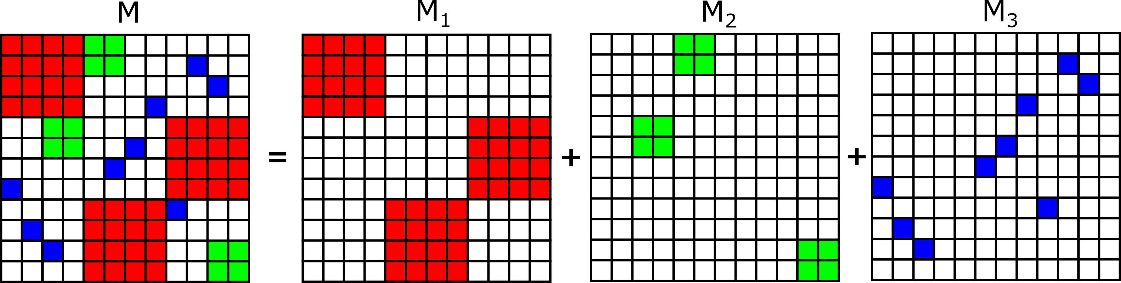
Figure 1: Hierarchical block sparse(HBS) configuration with 3 levels[(4x4),(2x2) and (1x1)].

2.3 Pruning methodology

For a given matrix $I$, block dimensions $(bh,bw)$ and sparsity $sp$, block sparsity is generated by dividing the matrix $I$ into a grid, where each grid element is of size $(bh,bw)$. Each grid element is then given a rank using the absolute summation values of that grid block. We then sort these values and prune away $sp$ % of blocks to generate a block sparse matrix. In case of hierarchical block sparsity with $N$ levels, block sizes $BS=[(bh_{1},bw_{1}),\dots(bh_{N},bw_{N})]$ and sparsities $SP={sp_{1},\dots sp_{N}}$ are provided for all the levels. Let $I_{k}$ and $M_{k}$ be the input and output matrices at level $k$. In level $k$, we perform a block sparse pruning with block size $(bh_{k},bw_{k})$ and sparsity $sp_{k}$ to generate $M_{k}$. We then generate input to layer $k+1$ by removing elements of $M_{k}$ from $I_{k}$ i.e, $I_{k+1}=I_{k}-M_{k}$. Figure 2, shows an example of 2 level HBS pruning on 4x4 matrix with BS=[(2,2),(1,1)] and SP=[50,75]. In case of networks where parameters of a layer are arranged in more than two dimensions, block dimensions correspond to outer two dimensions. For example, in case of CNNs, blocking is performed on ofm(output feature maps) and ifm(input feautre maps).

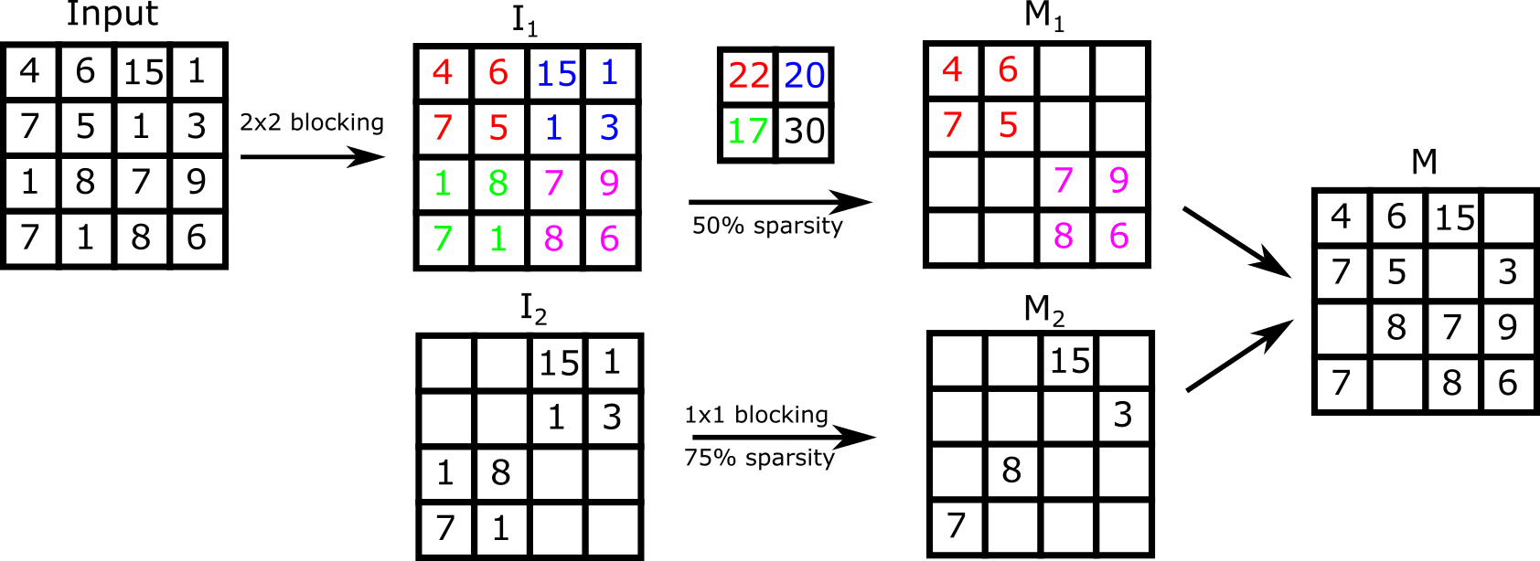
Figure 2: 2-Level block sparse generation : Block sizes=[(2x2),(1x1)] sparsities=[50,75]

2.4 Performance model

In this section, we describe a performance model for evaluating performance of a layer in HBsNN. For a given HBS configuration, let $F_{dense}$ and $F_{sparse}$ be the amount of compute for dense and sparse operations respectively. As a layer in HBsNN has multiple levels($L_{1},\dots,L_{N}$), $F_{sparse}=\sum_{i=1}^{i=N}F_{sparse}^{L_{i}}$, where $F_{sparse}^{L_{i}}$ is the amount of compute in $i^{th}$ level of the layer. Due to irregularity in sparse computation, it is not always possible to realize the ideal speed up i.e, $F_{dense}/F_{sparse}$. The achievable speedup depends primarily on two factors: 1)Amount of sparsity and 2)Dimensions of blocks. We quantify the sub-optimal speedup with an irregular factor function $irf(sparsity,blockDimensions)$ parameterized by those two factors. By taking these factors into effect, the cost of dense($C_{dense}$), and the cost of sparse neural network($C_{sparse}$) are defined according to equation 1 and 2. Achievable speedup can then be defined as $C_{dense}/C_{sparse}$. $irf(\dots)$ function varies from a system to system and has to be obtained by running micro benchmarks on that system. But on a regular parallel hardware such as TPU, $irf$ function is inversely proportional to block size. So, inorder to maximize performance, one needs to maximize sparsity for levels with smaller block sizes, and minimize sparsity for levels with larger block sizes.

$$C_{dense}=F_{dense}$$ (1)

$$C_{sparse}=\sum_{i=1}^{i=N}\dfrac{F_{sparse}^{L_{i}}}{irf(Sparsity(L_{i}),BlockDims(L_{i}))}$$ (2)

$$SpeedUp=\dfrac{C_{dense}}{C_{sparse}}$$ (3)

3 Results

3.1 ResNet-v2-50/Imagenet

We took a pretrained Renset-v2-50 model with top-1 and top-5 accuracy of 76.13% and 92.86% respectively and then generated sparse models from it using prune and retrain methodology from Han et al. (2015). Except for the first convolution layer and the last fc layer, all layers are pruned. The pruned model is then trained for 18 epochs with the same set of hyper parameters as that of the pretrained model. The initial learning rate for training is set to ${1/100}^{th}$ of the base learning rate used for pretrained model. A step based learning rate decay is followed, where learning rate is decreased by a factor of 10 and 100 respectively at $9^{th}$ and $14^{th}$ epoch respectively.

Varying sparsity : In this experiment, we would like to study how accuracy varies with respect to sparsity. We vary sparsity from 50 to 87.50 with block size set to 1x1. From Table 3, we can see that accuracy decreases with sparsity and the rate at which it decreases is exponential. This is due to the fact that more number of elements are pruned away with increase in sparsity and this reduces the model capacity.

Sparsity	Top-1 Accuracy	Top-5 Accuracy
50	76.42 (+0.29)	93.03 (+0.17)
75	75.12 (-1.01)	92.34 (-0.52)
87.50	71.58 (-4.55)	90.58 (-2.28)

Table 3: Varying sparsity with block size set to 1x1.

Varying block size : In this experiment, we would like to study how accuracy varies with respect to block size. Other parameters like sparsity and number of levels are kept same. From Table 4 and 5, we can see that accuracy decreases with increase in block size. This is due to the fact that as we increase block size, more number of high magnitude elements are pruned away due to increased structural constraint.

Block-size	Top-1 Accuracy	Top-5 Accuracy
4x1	75.73 (-0.40)	92.70 (-0.16)
8x1	75.19 (-0.94)	92.49 (-0.37)
16x1	75.03 (-1.10)	92.36 (-0.50)
32x1	74.52 (-1.61)	91.99 (-0.87)

Table 4: Varying block size with sparsity set to 50%.

Block-size/sparsity		Accuracy
Level-1 (L1)	Level-2 (L2)	Top-1	Top-5
4x1/53	1x1/97	75.93 (-0.20)	92.81 (-0.05)
8x1/53	1x1/97	75.67 (-0.46)	92.65 (-0.21)
16x1/53	1x1/97	75.55 (-0.58)	92.75 (-0.11)
32x1/53	1x1/97	75.26 (-0.87)	92.48 (-0.38)

Table 5: Varying block size with two levels. (Cumulative-Sparsity=50)

Varying sparsity distribution: In this experiment, we set sparsity to 50% and distribute it across multiple levels with block sizes ranging from 32x1 to 1x1 in a hierarchical fashion. Each row in Table 6 corresponds to a Hierarchical block sparse configuration and we can see that accuracy increases by having more fluidity in the structure imposed on sparsity. Another way of bringing fluidity and retaining structure is through Quasi block sparse configuration, which is a subset of Hierarchical block sparse configuration. In this case, there are two levels where one level has block sparsity and another level has unstructured sparsity with block size 1x1. In Quasi block sparse configuration, block sparsity caters for performance and unstructured sparsity caters for accuracy. From Table 7, we can see that the accuracy increases with increase in fluidity and with minimal loss to accuracy, significant amount of compute can be made regular.

Sparsity					Accuracy
L1-(32x1)	L2-(16x1)	L3-(8x1)	L4-(4x1)	L5-(1x1)	Top-1	Top-5
50	-	-	-	-	74.52 (-1.61)	91.99 (-0.87)
75	75	-	-	-	74.85 (-1.28)	92.37 (-0.49)
75	87.50	87.50	-	-	75.18 (-0.95)	92.49 (-0.37)
75	-	75	-	-	75.22 (-0.91)	92.43 (-0.43)
75	87.50	93.75	93.75	-	75.31 (-0.82)	92.50 (-0.36)
75	-	-	75	-	75.44 (-0.69)	92.63 (-0.23)
75	87.50	93.75	96.875	96.875	75.63 (-0.50)	92.67 (-0.19)

Table 6: Hierarchical block structure with varying sparsity distribution. (Cumulative-Sparsity=50)

Sparsity		Accuracy
L1-(32x1)	L2-(1x1)	Top-1	Top-5
62.50	87.50	75.92 (-0.21)	92.79 (-0.07)
56.25	93.75	75.64 (-0.49)	92.62 (-0.24)
53	97	75.26 (-0.87)	92.48 (-0.38)

Table 7: Quasi block sparsity with varying sparsity distribution. (Cumulative-Sparsity=50)

4 Conclusion

In HBsNN models, levels with smaller block sizes cater for bridging accuracy gap and levels with larger block sizes cater for improving performance. Thus HBsNN models have better accuracies than highly structured sparse models and have better performance than unstructured sparse models. This fluidity in structure in HBsNN models is essential to obtain better sparse models which are both accurate and performant.

References

- Cun et al. (1990) Yann Le Cun, John S. Denker, and Sara A. Solla. Optimal brain damage. In Advances in Neural Information Processing Systems, pp. 598–605. Morgan Kaufmann, 1990.
- Han et al. (2015) Song Han, Jeff Pool, John Tran, and William Dally. Learning both weights and connections for efficient neural network. In Advances in neural information processing systems, pp. 1135–1143, 2015.
- Han et al. (2016) Song Han, Xingyu Liu, Huizi Mao, Jing Pu, Ardavan Pedram, Mark A. Horowitz, and William J. Dally. Eie: Efficient inference engine on compressed deep neural network. SIGARCH Comput. Archit. News, 44(3):243–254, June 2016. ISSN 0163-5964. doi: 10.1145/3007787.3001163. URL http://doi.acm.org/10.1145/3007787.3001163.
- Hassibi et al. (1993) Babak Hassibi, David G. Stork, and Stork Crc. Ricoh. Com. Second order derivatives for network pruning: Optimal brain surgeon. In Advances in Neural Information Processing Systems 5, pp. 164–171. Morgan Kaufmann, 1993.
- He et al. (2016) Kaiming He, Xiangyu Zhang, Shaoqing Ren, and Jian Sun. Identity mappings in deep residual networks. In European Conference on Computer Vision, pp. 630–645. Springer, 2016.
- Narang et al. (2017a) Sharan Narang, Gregory F. Diamos, Shubho Sengupta, and Erich Elsen. Exploring sparsity in recurrent neural networks. CoRR, abs/1704.05119, 2017a. URL http://arxiv.org/abs/1704.05119.
- Narang et al. (2017b) Sharan Narang, Eric Undersander, and Gregory F. Diamos. Block-sparse recurrent neural networks. CoRR, abs/1711.02782, 2017b. URL http://arxiv.org/abs/1711.02782.
- Parashar et al. (2017) Angshuman Parashar, Minsoo Rhu, Anurag Mukkara, Antonio Puglielli, Rangharajan Venkatesan, Brucek Khailany, Joel S. Emer, Stephen W. Keckler, and William J. Dally. SCNN: an accelerator for compressed-sparse convolutional neural networks. CoRR, abs/1708.04485, 2017. URL http://arxiv.org/abs/1708.04485.
- Szegedy et al. (2016) Christian Szegedy, Vincent Vanhoucke, Sergey Ioffe, Jon Shlens, and Zbigniew Wojna. Rethinking the inception architecture for computer vision. In Proceedings of the IEEE Conference on Computer Vision and Pattern Recognition, pp. 2818–2826, 2016.
- Wen et al. (2016) Wei Wen, Chunpeng Wu, Yandan Wang, Yiran Chen, and Hai Li. Learning structured sparsity in deep neural networks. In Proceedings of the 30th International Conference on Neural Information Processing Systems, NIPS’16, pp. 2082–2090, USA, 2016. Curran Associates Inc. ISBN 978-1-5108-3881-9. URL http://dl.acm.org/citation.cfm?id=3157096.3157329.