Localization and delocalization of fermions in a background of correlated spins

Abstract

We study the (de)localization phenomena of one-component lattice fermions in spin backgrounds. The O(3) classical spin variables on sites fluctuate thermally through the ordinary nearest-neighbor coupling. Their complex two-component (CP¹-Schwinger boson) representation forms a composite U(1) gauge field on bond, which acts on fermions as a fluctuating hopping amplitude in a gauge invariant manner. For the case of antiferromagnetic (AF) spin coupling, the model has close relationship with the $t$-$J$ model of strongly-correlated electron systems. We measure the unfolded level spacing distribution of fermion energy eigenvalues and the participation ratio of energy eigenstates. The results for AF spin couplings suggest a possibility that, in two dimensions, all the energy eigenstates are localized. In three dimensions, we find that there exists a mobility edge, and estimate the critical temperature $T_{\rm\scriptscriptstyle{L}D}(\delta)$ of the localization-delocalization transition at the fermion concentration $\delta$.

I Introduction

Localization-delocalization (LD) transition of fermions has been one of the most important problems in quantum statistical physics and random systems. After the seminal work by Anderson anderson , its relation to the scaling theory, nonlinear sigma models, and the universality class of random matrix theory have been studied extensively matrix . The effect of interactions among fermions on the localization has been studied mostly by using the perturbation theory fukuyama . Recently, effects of strong correlations between fermions on a localization have attracted interests in modern perspectives. Among others, Smith et al.smith1 considered fermions in one dimension (1D) coupled with the $z$-component of $s=1/2$ spins, and studied many-body localization (MBL) driven by spontaneously generated disorders and its relation to disentanglement, etc.

As another interesting work, Kovacs et.al. kovacs studied a LD-like transition in quantum chromodynamics (QCD) by directly analyzing the eigenstates of relativistic kernel of quarks moving in gluon backgrounds. They employed a quenched approximation; i.e., gluon configurations are generated by the SU(N) pure gauge theory, ignoring the back-reaction by quarks. This system is substantially different from the Anderson model on the following points; (i) the background gluon field acts on fermions not as a random site potential but as a fluctuating hopping amplitude on link, and (ii) the hopping amplitudes are not independent link by link but correlate each other via the SU(N) gauge-field dynamics. QCD is a strong-coupling system due to large fluctuations of gluons, and it is regarded as a strongly-correlated system, even though there exist no self-couplings of quarks.

Recently, there appeared a couple of interesting systems sharing similar properties to the above mentioned QCD. The spin model by Kitaev kitaev is represented in terms of Majorana fermions moving in a static Z(2) gauge field. Smith et.al. smith2 introduced fermion models coupled with a Z(2) gauge field to study the MBL, focusing on the role of local gauge symmetry.

The purpose of the present work is to study yet another type of random-gauge system; spinless fermions coupled with a composite U(1) gauge field, which comes from the Schwinger-boson (CP¹) representation of the O(3) spins. This gauge theory of fermions is not only simple and universal but also is closely related with the $t$-$J$ model tjmodel of strongly-correlated electron system in the slave-fermion representation sf1 ; sf . Strong interactions between electrons induce fluctuating spin degrees of freedom with nontrivial correlations. In this perspective, the fermions in the present model are nothing but doped holes in the spin background. As far as we know, the problem of localization of doped holes in strongly-correlated electron systems has not been addressed yet.

In this work, we shall study the system in two and three spatial dimensions by numerically measuring quantities concerning to the localization phenomena. These numerical studies show that this system exhibits a LD transition in three dimensions (3D) for the antiferromagnetic (AF) case, and we estimate the critical temperature of the LD transition as a function of the fermion concentration. Together with the numerical results for the ferromagnetic (FM) case, we suggest a coherent structure of the phase diagram of LD transition.

This paper is organized as follows. In Sec. II, we introduce the target model and explain its relation to the $t$-$J$ model of strongly-correlated electrons. In the model, a spinless fermion moves in the spin background with nontrivial O(3) correlations. We also explain the outline how to prepare the spin configurations and use them to calculate physical quantities studied in the successive sections. In Sec. III, we show the numerical results of the unfolded level spacing distribution (ULSD) for the 2D and 3D cases. We find that the system-size dependence of ULSD reveals an important difference in the 2D and 3D cases, which allows us to determine the location of the mobility edge for the 3D system. In Sec. IV, we investigate the participation ration (PR), which is another useful quantity used for the study on LD transitions. Numerical results verify the observations obtained in Sec. III. In Sec. V, we use these results to locate the LD transition temperature as a function of fermion concentration. In Sec. VI, we present the results for the FM spin background, and discuss a possible behavior of the LD transition temperature. Section VII is devoted for conclusion.

II Model

Before going to study on the target model, let us consider the Anderson model to fix the notations and concepts that we will use in the rest of this work. The Hamiltonian of the Anderson model is given as follows anderson ;

$$\hat{H}_{\rm\scriptscriptstyle{A}}=-t\sum_{x,i}\left(\hat{\psi}^{\dagger}_{x+i}\hat{\psi}_{x}+{\rm H.c.}\right)+\sum_{x}V_{x}\hat{\psi}^{\dagger}_{x}\hat{\psi}_{x},$$ (2.1)

where $\hat{\psi}_{x}$ is the annihilation operator of fermion at site $x$ of the $D$-dimensional lattice without self-interactions, satisfying $[\hat{\psi}_{x},\hat{\psi}^{\dagger}_{y}]_{+}=\delta_{xy}.$ $t$ is the hopping amplitude from $x$ to $x\pm i$ with $i=1,\cdots,D$. $V_{x}$ is a random potential distributing uniformly in $[-\frac{U}{2},+\frac{U}{2}]$. We measure the energy eigenvalue $\lambda$ of $\hat{H}_{\rm\scriptscriptstyle{A}}$ from the band center ($\lambda=0$). For $D=2$, all the energy eigenstates for $U>0$ are localized, while in 3D, there exists a mobility edge (ME) at $\lambda=\pm\lambda_{\rm\scriptscriptstyle{ME}}(U)$ ucrit . ME separates extended states for $-\lambda_{\rm\scriptscriptstyle{ME}}<\lambda<\lambda_{\rm\scriptscriptstyle{ME}}$ and localized states for $|\lambda|>\lambda_{\rm\scriptscriptstyle{ME}}$. Fermi energy $\lambda_{\rm\scriptscriptstyle{F}}(\delta)$ is an increasing function of fermion density $\delta\ (\equiv$ average fermion number/site). The critical density $\delta_{c}$ of the LD transition is defined by $\lambda_{\rm\scriptscriptstyle{F}}(\delta_{c})=-\lambda_{\rm\scriptscriptstyle{ME}}$. Then as $\delta$ crosses $\delta_{c}$ from below, there appear extended states. If fermions are charged, the system changes from an insulator to a metal at $\delta=\delta_{c}$. The energy spectrum of the target model has a similar structure to that of the Anderson model. The primary concern is whether the ME exists or not.

The Hamiltonian of the target model $\hat{H}_{\psi}$ is given by

$$\hat{H}_{\psi} = -t\sum_{x,i}\left(Q_{xi}\hat{\psi}^{\dagger}_{x+i}\hat{\psi}_{x}+{\rm H.c.}\right),$$

$$Q_{xi} \equiv \bar{z}_{x}z_{x+i}=\sum_{\sigma=1}^{2}{z}^{*}_{x\sigma}z_{x+i,\sigma}.$$ (2.2)

Hereafter, we put $t=\frac{1}{2}$ as the unit of energy. The complex fermion hopping amplitude $Q_{xi}$ is defined on each link $(x,x+i)$ in terms of the CP¹ variable cp1 or Schwinger bosons $z_{x\sigma}$. $z_{x\sigma}\ (\sigma=1,2)$ is the two-component complex site variables on $x$ and satisfies the following local constraint;

$$z_{x} = (z_{x1},z_{x2})^{\rm t},\ z_{x\sigma}(\sigma=1,2)\in{\bf C}$$

$$\bar{z}_{x}z_{x} \equiv \sum_{\sigma}z^{*}_{x\sigma}z_{x\sigma}=1.$$ (2.3)

(The bar symbol denotes Hermitian conjugate.) This $z_{x}$ forms a background classical O(3) spin vector $\vec{S}_{x}$ as

$$\vec{S}_{x}=\bar{z}_{x}\vec{\sigma}z_{x},\ \vec{S}_{x}\cdot\vec{S}_{x}=1,$$ (2.4)

where $\vec{\sigma}$ are the Pauli matrices.

The target Hamiltonian $\hat{H}_{\psi}$ in Eq. (2.2) can be regarded as a model describing dynamics of holes doped in many-body spin degrees of freedom that are generated by the strong correlations between electrons. A typical model of such strongly-correlated electron systems is the $t$-$J$ model tjmodel whose Hamiltonian is given as

$$\hat{H}_{tJ} = -t\sum_{x,i,\sigma}\left(\tilde{C}_{x+i,\sigma}^{\dagger}\tilde{C}_{x\sigma}+{\rm H.c.}\right)$$ (2.5)

$$+ J\sum_{x,i}\left(\hat{\vec{S}}_{x+i}\hat{\vec{S}}_{x}-\frac{1}{4}\hat{n}_{x+i}\hat{n}_{x}\right),$$

$$\tilde{C}_{x\sigma} \equiv \left(1-\hat{C}^{\dagger}_{x\bar{\sigma}}\hat{C}_{x\bar{\sigma}}\right)\hat{C}_{x\sigma},$$ (2.6)

$$\hat{\vec{S}}_{x} \equiv \frac{1}{2}\hat{C}^{\dagger}_{x}\vec{\sigma}\hat{C}_{x},\ \hat{n}_{x}\equiv\sum_{\sigma}\hat{C}^{\dagger}_{x\sigma}\hat{C}_{x\sigma},$$

where $\hat{C}_{x\sigma}$ is the annihilation operator of electron at the site $x$ with the spin $\sigma=1(\uparrow),2(\downarrow)$, and $\bar{\sigma}=1(2)$ for $\sigma=2(1)$. The physical states of the $t$-$J$ model exclude the double-occupancy states such as $\hat{C}^{\dagger}_{x\uparrow}\hat{C}^{\dagger}_{x\downarrow}|0\rangle$ due to the strong electron correlations, i.e, the strong on-site repulsion of electrons. Due to this local constraint, the specific operators $\tilde{C}_{x\sigma}$ in Eq. (2.6) have been introduce and the hopping term in Eq. (II) is expressed in terms of them. The same on-site repulsion also induces the spin-spin interaction in $\hat{H}_{tJ}$ in Eq. (2.5).

The local constraint is faithfully treated by using the slave-fermion representation sf1 ; sf . In the slave-fermion representation of electron, $\hat{C}_{x\sigma}$ is represented as a composite,

$$\hat{C}_{x\sigma}=\hat{\psi}_{x}^{\dagger}\hat{a}_{x\sigma},$$ (2.7)

where $\psi_{x}^{\dagger}$ is the creation operator of one-component fermionic hole [we use the same notation $\psi_{x}$ as the fermion operator in Eq. (2.2) because they are to be regarded as the same thing] and $a_{x\sigma}$ is the annihilation operator of two-component bosonic spin. The physical states are defined by imposing the no-double occupancy condition such as,

$$\sum_{\sigma}\hat{a}_{x\sigma}^{\dagger}\hat{a}_{x\sigma}+\hat{\psi}_{x}^{\dagger}\hat{\psi}_{x}=1.$$ (2.8)

We introduce a set of bosonic operators, $z_{x\sigma}$, and the following parametrization;

$$\hat{a}_{x\sigma} = (1-\hat{\psi}^{\dagger}_{x}\hat{\psi}_{x})^{1/2}\hat{z}_{x\sigma}$$ (2.9)

$$= (1-\hat{\psi}^{\dagger}_{x}\hat{\psi}_{x})\hat{z}_{x\sigma},$$

where we have used the fact that the eigen-values of $\hat{\psi}^{\dagger}_{x}\hat{\psi}_{x}$ are $0$ and $1$. Then, Eq. (2.8) is reduced to the so-called CP¹ constraint,

$$\sum_{\sigma}\hat{z}^{\dagger}_{x\sigma}\hat{z}_{x\sigma}=1.$$ (2.10)

It is rather straightforward to derive the Hamiltonian $\hat{H}_{\psi}$ in Eq. (2.2) from the hopping term in $\hat{H}_{tJ}$ in Eq. (2.5). In particular, for the low doping case, where the hole concentration $\delta=\langle\hat{\psi}^{\dagger}_{x}\hat{\psi}_{x}\rangle$ is small, one may set $\hat{a}_{x}\simeq\hat{z}_{x}$ in Eq. (2.9) and the electron hopping term in Eq. (2.5) becomes smalldelta

$$\tilde{C}_{x+i,\sigma}^{\dagger}\tilde{C}_{x\sigma}+\mbox{H.c.}\to\hat{z}^{\dagger}_{x+i,\sigma}\hat{\psi}_{x+i}\hat{\psi}^{\dagger}_{x}\hat{z}_{x\sigma}+\mbox{H.c.}$$ (2.11)

This is just the hopping term of the Hamiltonian $\hat{H}_{\psi}$ of Eq. (2.2).

In the present work, we treat $\{z_{x}\}$ in $\hat{H}_{\psi}$ as random variables obeying certain distribution density $\rho(z)$. Explicitly we take $\rho(z)$ as the Boltzmann distribution at the temperature $T$ with the energy $E_{z}$ of the following O(3) spin model;

$$E_{z}=-J\sum_{x,i}\vec{S}_{x+i}\cdot\vec{S}_{x},$$

$$\rho(z)=\frac{\exp(-\beta E_{z})}{\int[dz]\exp(-\beta E_{z})},$$ (2.12)

where $J$ is the ferromagnetic (FM $J>0$) or AF ($J<0$) exchange coupling, $\beta\equiv 1/(k_{\rm\scriptscriptstyle{B}}T)$, and $[dz]=\prod_{x}dz_{x}$ is the Haar measure. Eq. (2.12) is obviously motivated by the spin-spin interactions in the $t$-$J$ model in Eq. (2.5) sgnj . It should be remarked here that the above treatment of the spin and hole variables is motivated by the recent works on MBL for systems in which fast and slow particles exist and slow particles serve as a random quasi-static background potential for fast particles Schiulaz ; yao . Namely, our treatment is viewed as a quenched approximation for the total Hamiltonian $\hat{H}_{\psi z}=\hat{H}_{\psi}+E_{z}$ regarding $\{z_{x}\}$ as quenched variables and neglecting the back-reaction from fermions to spins. It is quite straightforward to extend the present formalism to other cases of spin correlation. In the practical calculation below, we prepare $M(\simeq 1000)$ such $z$-samples, each of which is chosen in every 10 sweeps of the Hybrid Monte Carlo simulations.

$\hat{H}_{\psi}$ of Eq. (2.2) and $\vec{S}_{x}$ of Eq. (2.4) are invariant under the local U(1) gauge transformation cinv ,

$$z_{x\sigma}\to e^{i\varphi_{x}}z_{x\sigma},\hat{\psi}_{x}\to e^{i\varphi_{x}}\hat{\psi}_{x},$$ (2.13)

where $\varphi_{x}$ is an arbitrary phase for a local gauge transformation. This way to couple fermions with O(3) spins $\vec{S}_{x}$ by introducing $z_{x}$ in a gauge-invariant manner reminds us the well known way to couple charged particles with electromagnetic field by introducing gauge field $A_{x\mu}$. Because $\psi_{x}$ represents doped holes in Ref. sf1 ; sf , the present model may have some universality common to hole-doped spin models. In the present work, we study the simplest case in Eq. (2.12).

We consider the $D$-dimensional spatial lattice with $N=L^{D}$ sites and the periodic boundary condition. For each $z$-sample, we calculate numerically $N$ eigenvalues $\lambda$ and eigenfunctions $\phi_{x}(\lambda)$ of the Hermitian fermion kernel $\Gamma$ in $\hat{H}_{\psi}$,

$$\hat{H}_{\psi} = \sum_{x,y}\hat{\psi}^{\dagger}_{x}\Gamma_{xy}(z)\hat{\psi}_{y},$$

$$\Gamma_{xy} = -\frac{1}{2}\sum_{i}\bar{z}_{y}z_{x}(\delta_{y,x-i}+\delta_{y,x+i}).$$ (2.14)

In the eigenvalue equation,

$$\sum_{y}\Gamma_{xy}\phi_{y}(\lambda)=\lambda\phi_{x}(\lambda),$$ (2.15)

$\Gamma_{xy}$ and $\phi_{x}$ gauge-transform covariantly as $\Gamma_{xy}\to e^{i\varphi_{x}}\Gamma_{xy}e^{-i\varphi_{y}}$ and $\phi_{x}\to e^{i\varphi_{x}}\phi_{x}$, whereas $\lambda$’s are gauge-invariant. By using $\lambda$ and $|\phi_{x}(\lambda)|$, we calculate the ULSD and PR. Then, we average these quantities over $M$ $z$-samples. The obtained results give important informations about (de)localization of fermions $\hat{\psi}_{x}$.

To understand the $\beta$-dependence of the results given below, it is useful to recall that the O(3) spin model (2.12) has a symmetry under AF $\leftrightarrow$ FM with $J\leftrightarrow-J$, and the 2D model has only the paramagnetic (PM) phase, whereas the 3D model exhibits the second-order AF(FM)-PM phase transition at $\beta J\simeq-1.4(1.4)$. The two amplitudes on the link $(x,x+i)$, (i) FM spin-pair amplitude $Q_{xi}=\bar{z}_{x}z_{x+i}$ and (ii) AF(resonating-valence bond) amplitude,

$$R_{xi}\equiv z_{x1}z_{x+i,2}-z_{x2}z_{x+i,1},$$ (2.16)

satisfy the identity,

$$|Q_{xi}|^{2}+|R_{xi}|^{2}=1,$$ (2.17)

and the each term in $E_{z}$ is expressed as $\vec{S}_{x+i}\cdot\vec{S}_{x}=|Q_{xi}|^{2}-|R_{xi}|^{2}=1-2|R_{xi}|^{2}=2|Q_{xi}|^{2}-1$.

As $\beta J$ increase from $-\infty$ (deep AF phase) to $\infty$ (deep FM phase), the average squared magnitude $\langle|Q_{xi}|^{2}\rangle$ increases monotonically from zero to 1. In particular, in the strong paramagnetic phase ($|\beta J|\sim 0$), $\langle|Q_{xi}|^{2}\rangle\simeq\langle|R_{xi}|^{2}\rangle\simeq\frac{1}{2}$. Generally speaking, as we see below, the population of delocalized states (if any) in the whole spectrum increases as $|Q_{xi}|$ increases.

III Unfolded level spacing distribution (ULSD)

III.1 Definition of ULSD

The ULSD is one of the commonly used quantities matrix ; kovacs to find a ME in an energy spectrum. Due to the sublattice symmetry of the system (2.14), $\lambda$’s distribute symmetrically around $\lambda=0$, and we focus on the half of them ($\lambda\geq 0$). For each $z$-sample, we sort $N/2$ $\lambda$’s as $\lambda_{m}\ (m=1,\cdots,N/2$) with $\lambda_{m}\leq\lambda_{m+1}$. We group these $\lambda$’s into $K$ successive sets (cells) $C_{k}(k=1,\cdots,K)$ such that $C_{k}$ contains $\Lambda_{k}$ successive $\lambda$’s as $C_{k}=(\lambda^{k}_{1},\cdots,\lambda^{k}_{\Lambda_{k}})$, where $\lambda^{k}_{\alpha}\equiv\lambda_{T_{k}+\alpha}$ with $T_{k}\equiv\sum_{\ell=1}^{k-1}\Lambda_{\ell}$. For each $C_{k}$, we introduce $\Lambda_{k}-1$ unfolded level spacings $s^{k}_{\alpha}\ (\alpha=1,\cdots,\Lambda_{k}-1)$ defined as

$$s^{k}_{\alpha} \equiv \frac{\lambda^{k}_{\alpha+1}-\lambda^{k}_{\alpha}}{\Delta\lambda^{k}},\ \Delta\lambda^{k}\equiv\frac{\lambda^{k}_{\Lambda_{k}}-\lambda^{k}_{1}}{\Lambda_{k}-1},$$ (3.1)

where $\Delta\lambda^{k}$ is the average of the $(\Lambda_{k}-1)$ nearest-neighbor level spacings over $C_{k}$.

Then we assemble these $s\ (=\{s^{k}_{\alpha}\})$ for each cell $C_{k}$ over $M$ $z$-samples, and calculate their distribution $P_{k}(s)$. By definition, $P_{k}(s)$ satisfies the following identities;

$$\int_{0}^{\infty}dsP_{k}(s)=1,\ \ \int_{0}^{\infty}dssP_{k}(s)=1$$ (3.2)

(owing to the unfolding). In the following calculations, we choose the parameters as $K=40,\Lambda_{k}\simeq N/(2K)$.

In the random matrix theory matrix , typical behaviors of $P(s)$ ($=P_{k}(s)$ for each cell $C_{k}$ in the present context) are known as

$${\rm Poisson\ type}\ P_{\rm\scriptscriptstyle{P}}(s)\propto\exp(-s),$$ (3.3)

$${\rm Wigner\ type}\ P_{\rm\scriptscriptstyle{W}}(s)\propto s^{c}\exp(-ds^{2}),$$

with certain positive constants $c$ and $d$. The behavior of $P_{k}(s)$ near $s\simeq 0$ clarifies whether the eigenstates in the $k$-th cell are localized or extended, i.e.,

$$P_{k}(0)\left\{\begin{array}[]{ll}\neq 0,&{\rm Poisson,\ localized\ state}\\ \simeq 0,&{\rm Wigner,\ extended\ state.}\\ \end{array}\right.$$ (3.6)

Because localized eigenstates have a same shape with a finite extension (localization length) and to be distinguished by their locations (centers). These states are degenerate in energy $(s=0)$, giving rise to $P_{k}(0)>0$. On the other hand, extended eigenstates are made of superpositions of localized basis states as in Bloch wave so that the degeneracy is removed $P_{k}(0)=0$. As $K$ becomes sufficiently large, one can identify the ME as $\lambda_{\rm\scriptscriptstyle{ME}}\simeq\lambda^{k}_{1}$ where $P_{k}(0)\sim 0$ and $P_{k+1}(0)\neq 0$. The whole range of positive $\lambda$ axis is partitioned into the following sections; (i) extended states; $0\leq\lambda\leq\lambda_{\rm\scriptscriptstyle{ME}}$, (ii) localized states; $\lambda_{\rm\scriptscriptstyle{ME}}<\lambda\leq\lambda_{\rm\scriptscriptstyle{M}AX}$, (iii) no states; $\lambda_{\rm\scriptscriptstyle{M}AX}<\lambda$.

III.2 Results of ULSD

Let us turn to numerical results. In Fig. 1, we show 2D AF ULSD, $P_{k}(s)$, for various linear lattice sizes $L$. Fig. 1(a) for $\beta J=-0.1$ shows that $P_{k}(s)$’s with both $k=2$ and $k=40$ look the Wigner type for $L=12$. However, the curve for $k=40$ seems to approach to the Poisson type as $L$ increases. In Fig. 1(b), we show $P_{k}(s_{0})$, where $s_{0}$ is the smallest value of $s$ in each cell $C_{k}$. $P_{k}(s_{0})$ shows that this $L$-dependence is systematic. That is, as $L$ increases, the region of $k$ with the Poisson type increases toward the lower $k$ monotonically. Figs. 1(c) and (d) for $\beta J=-10.0$ slightly amplify this $L$-dependence as expected because localization is more favored than $\beta J=-0.1$. This peeling-off phenomenon continues down to some value $k=k_{c}$ in $L\to\infty$, and then $k_{c}$ is the ME, although the precise determination of $k_{c}$ by $P_{k}(s_{0})$ alone requires scaling arguments using the date for larger $L$’s. We shall discuss the ME by using more efficient methods below.

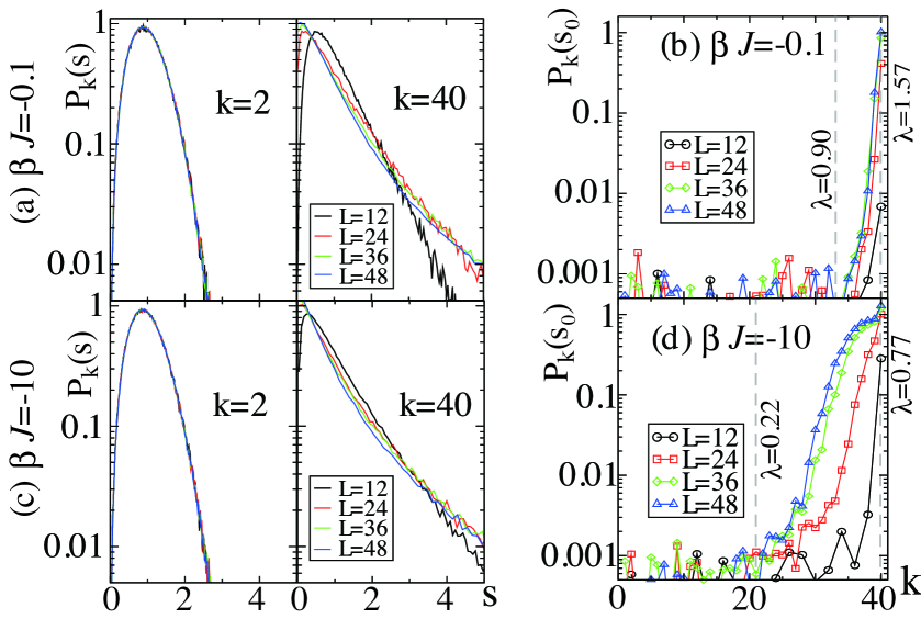
Figure 1: 2D AF ULSD $P_{k}(s)$ ($K=40$) for various $L$’s. (a) $P_{k}(s)$ for $k=2$ and 40 ($\beta J=-0.1$). For $L=12$, both $P_{k}(s)$’s look the Wigner type. However, as $L$ increases, $P_{40}(s)$ approaches to the Poisson type. (b) $P_{k}(s_{0})$ at $s_{0}$, the smallest value of $s$ ($s_{0}$ is $0.005\sim 0.015)$. The region of $k$ for the Poisson type [$P_{k}(s_{0})>0$] extends to lower $k$’s as $L$ increases. (c), (d) Same plots for $\beta J=-10.0$. They show similar but stronger $L$-dependence of $P_{k}(s_{0})$. The dashed lines in Figs. (b) (d) show the locations of $\lambda_{\rm\scriptscriptstyle{M}AX}(K=40)$ (Right) and possible $\lambda_{\rm\scriptscriptstyle{M}E}$ or a crossover suggested by the data up to $L=48$ (Left).

In Fig. 2, we show the results of 3D AF ULSD for $\beta J=-0.1$, and $-10.0$. Fig. 2(a) shows that, as $L$ increases, $P_{2}(s)$ remains the Wigner type, whereas $P_{40}(s)$ changes to the Poisson type. $P_{k}(s_{0})$ in Fig. 2(d) for $\beta J=-10.0$ shows that the regions of lower and higher value of $P_{k}(s_{0})$ are more clearly separate than the 2D case of Fig. 1(d).

The above observation by using the ULSD seems to indicate that, both in the 2D and 3D cases, a LD transition or a crossover takes place at finite $\lambda_{\rm\scriptscriptstyle{ME}}$. As mentioned, we shall see that further analyses below provide us with certain signals for differences in the LD properties of the 2D and 3D systems.

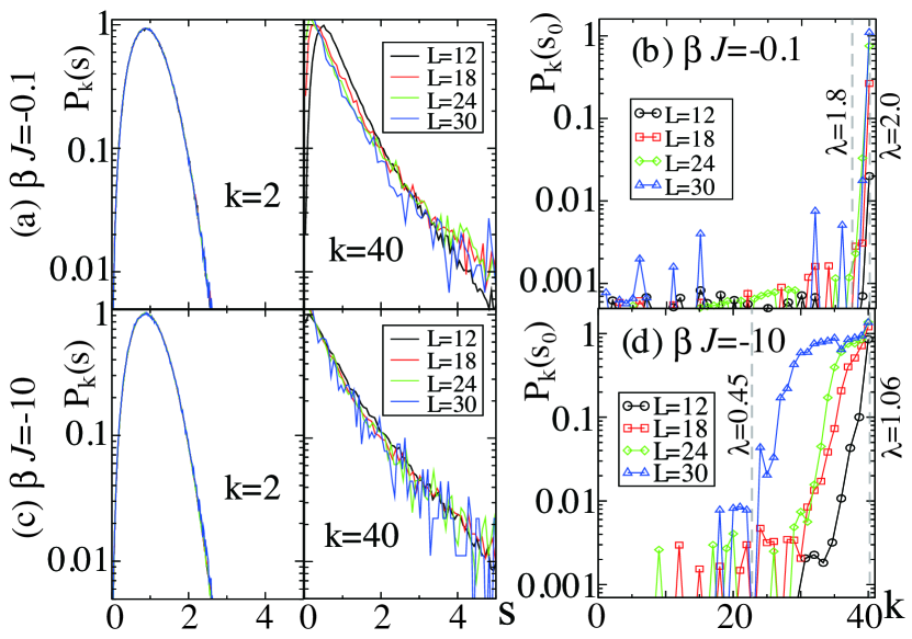
Figure 2: ​3D AF ULSD $P_{k}(s)$ ($K\!=\!40$) for various $L$’s. ​​​(a) $P_{k}(s)$ for $k=2$ and 40 ($\beta J=-0.1$). As $L$ increases, $P_{40}(s)$ approaches to the Poisson type, while $P_{2}(s)$ remains in the Wigner type. (b) $P_{k}(s_{0})$ ($\beta J=-0.1$). Its high-value region looks narrower than the 2D case of Fig. 1(b). (c),(d) Same plots for $\beta J=-10.0$. $P_{k}(s_{0})$ there separates its high-value region and low-value region at $k\sim 23$ more sharply than Fig. 2(d) of the 2D case with long tails, suggesting a ME. For the dashed lines, see Fig. 1.

III.3 ULSD and Mobility edge

A way to determine the location of ME, $\lambda_{\rm\scriptscriptstyle{ME}}$, in a systematic manner was proposed in Refs. kovacs ; integral . It uses the following integral;

$$I_{k}=\int_{0}^{\bar{s}}dsP_{k}(s),$$ (3.7)

where we put $\bar{s}\simeq 0.508$ 508 in the practical calculation following Refs. kovacs ; integral ; 196 , but the qualitative results are the same for other values of $\bar{s}(\approx 0.5)$. Physical meaning of the integral $I_{k}$ is the following. For small $\bar{s}$, $I_{k}$ picks up the behavior of $P_{k}(s)$ in the regime $s\sim 0$, so $I_{k}$ is small for the Wigner distribution and large for the Poisson distribution. Let us regard $I_{k}$ as a function of the smallest $\lambda$ in $C_{k}$, i.e., $\lambda^{k}_{1}$ and define $I(\lambda^{k}_{1})\equiv I_{k}$. For large $K$, $\lambda^{k}_{1}$ becomes sufficiently dense, and so $I(\lambda^{k}_{1})$ becomes a smooth function $I(\lambda)$, which equals $I_{k}$ for $\lambda=\lambda^{k}_{1}$. As we mentioned above, one can determine $\lambda_{\rm\scriptscriptstyle{M}E}$, from the behavior of $I(\lambda)$. Explicitly, we compare below $I(\lambda)$ with its three typical values;

$$I_{\rm\scriptscriptstyle{W}} \simeq 0.12 \ {\rm for}\ P_{\rm\scriptscriptstyle{W}}(s),$$

$$I_{\rm\scriptscriptstyle{P}} \simeq 0.40 \ {\rm for}\ P_{\rm\scriptscriptstyle{P}}(s),$$

$$I_{c} \simeq 0.196 \ {\rm for}\ P_{c}(s),$$ (3.8)

where the first two correspond to the Wigner and Poisson distributions of Eq. (3.3), respectively integral ; 508 . On the other hand, $P_{c}(s)$ is the critical distribution at the transition point between them integral ; 196 .

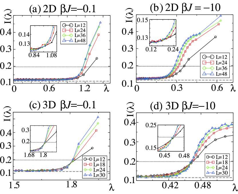
Figure 3: $I(\lambda)$ of Eq.(3.7) for $\beta J=-0.1,-10.0$. (a), (b) 2D $I(\lambda)$. For both $\beta$’s, as $L$ increases, $I(\lambda)$ peels off upward monotonically. (c), (d) 3D $I(\lambda)$. For both $\beta$’s, four curves with different $L$’s cross approximately at a single point in contrast with the 2D case. This almost $L$-independent point is a candidate of ME. The lower dashed lines show $I_{\rm\scriptscriptstyle{W}}$ and the upper dashed lines show $I_{c}$ of the critical statistics $P_{c}(s)$.

In Fig. 3, we show $I(\lambda)$ for $\beta J=-0.1$, and $-10.0$ and various $L$’s. In Figs. 3(a) and (b), 2D $I(\lambda)$ remains near the value $I_{\rm\scriptscriptstyle{W}}$ in the lower-$\lambda$ region, and it starts to deviate upward as $\lambda$ increases. As $L$ increases, the point of deviation shifts to lower $\lambda$’s monotonically.

In Figs. 3(c) and (d), 3D $I(\lambda)$ increases toward $I_{\rm\scriptscriptstyle{P}}$ as $\lambda$ increases, as expected ipoisson . The four curves of $I(\lambda)$ for four $L$’s show systematic size-dependence such that the transition gets sharper as $L$ increases, and interestingly enough, these four curves seem to cross with each other almost at the same point [Insets of Figs. 3(c) and (d)]. This is in sharp contrast with the 2D case. This crossing point is $L$-independent and to be a candidate for the ME in the infinite-volume limit. Another candidate of the ME is given by $I(\lambda_{\rm\scriptscriptstyle{M}E})=I_{\rm c}$ for the critical statistics at the transition point between the Poisson and the Wigner distributions, although the critical statistics itself of the present model may differ from $P_{c}(s)$ due to the correlated hopping. It is interesting that the above two methods give almost the same estimation of $\lambda_{\rm\scriptscriptstyle{ME}}$.

IV Participation ratio (PR)

Another quantity that we use to study the LD transition is the PR kovacs ; prn , which is defined by using a normalized eigenfunction $\phi_{x}$ of eigenvalue $\lambda$ as follows;

$${\rm PR}(\lambda)=\frac{1}{\sum_{x}|\phi_{x}|^{4}\cdot N}.$$ (4.1)

To see typical behavior of the PR, let us calculate PR of a state with $|\phi_{x}|^{2}=$ constant on $S$ sites and $\phi_{x}=0$ on the other $(N-S)$ sites;

$$\sum_{x}|\phi_{x}|^{2} = S\cdot|\phi_{x}|^{2}=1,\ {\rm PR}=\frac{1}{S\cdot S^{-2}\cdot N}=\frac{S}{N}.$$ (4.2)

Eq. (4.2) shows that ${\rm PR}$ is the ratio of numbers of participated (occupied) sites and the total sites.

In Fig. 4(a), we show the averaged value of 2D AF PR($\lambda$) over $M$ $z$-samples for $\beta J=-0.1$ and $-10.0$. As $\beta$ increases, the width of PR [the range of $\lambda=(-\lambda_{\rm\scriptscriptstyle{M}AX},\lambda_{\rm\scriptscriptstyle{M}AX})]$ decreases reflecting the fact that the magnitude of the FM hopping amplitude $Q_{xi}$ reduces as the AF correlation increases. Although PR exhibits a crossover between high and low-value regions suggesting existence of a finite $\lambda_{\rm\scriptscriptstyle{ME}}$, PR decreases monotonically as $L$ increases for all $\lambda$’s. To study the $L$-dependence of PR($\lambda)$ systematically, we fit the obtained data of PR as

$${\rm PR}(\lambda)=CL^{\gamma(\lambda)}.$$ (4.3)

In Fig. 4(b), we show the exponent $\gamma(\lambda)$. It shows that $\gamma$ is negative $(\lesssim-0.3)$ for all $\lambda$’s, suggesting that the $L$-dependence is strong enough, and all the states get localized (PR$\to 0$) as $L\to\infty$. If the state consists of a single localized region with finite localization length $\ell$, $S$ in Eq. (4.2) is $\propto\ell^{D}\sim L^{0}$ and $\gamma\to-D$ as $L\to\infty$ b . $\gamma$ in Fig. 4(b) certainly converges to this value for $\lambda\gtrsim 0.4$.

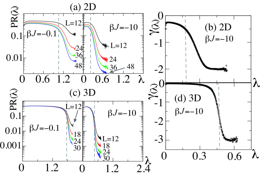
Figure 4: 2D and 3D AF PR($\lambda$). (a) 2D PR($\lambda$) for $\beta J=-0.1$ and $-10.0$. (We plot it only for $0\leq\lambda$ because PR$(\lambda)$ is an even function). In the small-$\lambda$ region, PR is fairly large corresponding to extended states, and as $\lambda$ increases, PR decreases rapidly toward localized states. As $L$ increases, PR’s for both $\beta J$ reduce monotonically in the entire region. (b) 2D exponent $\gamma(\lambda)$ in the fitting PR($\lambda$) = $CL^{\gamma}$. $\gamma(\lesssim-0.3)$ is negative for all $\lambda$, suggesting that PR $\to 0$ as $L\to\infty$. For large $\lambda$’s $\gamma$ converges to $-2(=-D)$ corresponding to localized states (See the text). The dashed lines in (a),(b) locate approximate crossover points. (c) 3D AF PR($\lambda$) for $\beta J=-0.1$ and $-10.0$. In contrast with the 2D PR of Fig.(a), $L$-dependence of PR in the small-$\lambda$ region is quite weak. (d) 3D exponent $\gamma(\lambda)$. It stays around zero for small $\lambda$’s and converges to $-D=-3$ for large $\lambda$’s. Figs. (c) and (d) suggest ME around the dashed lines.

In Fig. 4(c), we show 3D AF PR($\lambda$) for $\beta J=-0.1$ and $-10.0$. In contrast with the 2D PR in Fig. 4(a), the $L$-dependence in the small-$\lambda$ region is very weak and the location of the sharp reduction at $\lambda\simeq 0.47$ is stable, suggesting existence of a finite ME in the 3D case. In Fig. 4(d) we show the exponent $\gamma$. For $\lambda\lesssim 0.3$, $\gamma$ remains almost vanishing, suggesting the states in that regime are delocalized, and around $\lambda\simeq 0.47$, $\gamma$ shifts quickly to $\simeq-D$ of localized states. Therefore we conclude that there is a ME for $\beta J=-10.0$ at $\lambda_{\rm\scriptscriptstyle{M}E}\simeq 0.47$, and similarly $\lambda_{\rm\scriptscriptstyle{M}E}\simeq 1.8$ for $\beta J=-0.1$ [See the dashed lines in Figs. 4 (c) and (d)]. These values are in good agreement with the estimation by using $I(\lambda)$ of Figs. 3(c) and (d). We note that the 3D Anderson model has a similar behavior of PR$(\lambda)$, i.e., it has strong depression for localized states as $L$ increases, whereas it has almost no $L$-dependence for extended states.

Let us summarize the $L$-dependence of the AF 2D and 3D systems. Although $P_{k}$ in Figs. 1 and 2 show weaker signals, all the quantities, $P_{k}(s),I(\lambda)$, PR have similar behavior, i.e., the 2D system shows monotonic $L$-dependence, while the 3D system has some fixed point in $\lambda$ that indicates the existence of a ME. If the 2D monotonic behavior continues down to $\lambda\to 0$ as $L\to\infty$, all the states are to be localized.

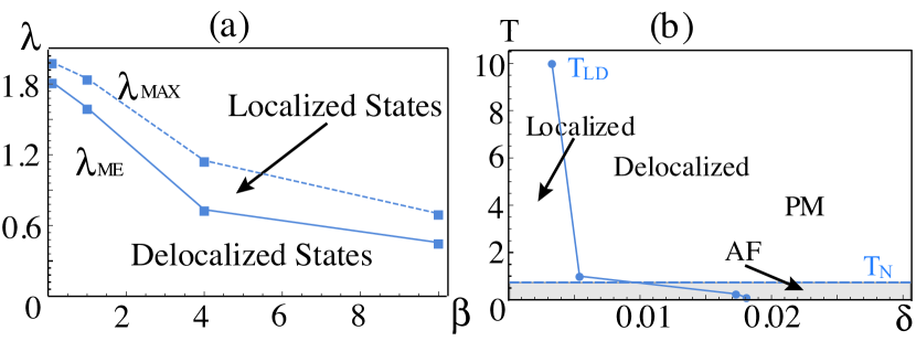
Figure 5: (a) 3D ME. $\lambda_{\rm\scriptscriptstyle{M}E}$ and $\lambda_{\rm\scriptscriptstyle{M}AX}$ vs. $\beta$ (we set $J=-1$). $\lambda_{\rm\scriptscriptstyle{M}E}$ are determined by $I(\lambda)$ of Fig. 3.7(c,d) and similar data for other $\beta$’s. (b) 3D $T_{\rm\scriptscriptstyle{L}D}(\delta)$ vs. $\delta-T$. The dashed line shows the Néel temperature $T_{\rm\scriptscriptstyle{N}}\simeq 1/1.4$ of the O(3) model of Eq. (2.12). In the AF phase, the region of localized states increases.

V Critical temperature of the LD transition

From the numerical studies explained in the previous sections, we can estimate the LD transition temperature as a function of the fermion concentration $\delta$. This problem is addressed in this section.

As the fermion concentration $\delta$ increases from zero to the critical density $\delta_{\rm c}$, Fermi energy increases from $-\lambda_{\rm\scriptscriptstyle{M}AX}$ to $-\lambda_{\rm\scriptscriptstyle{M}E}$. Because $\lambda_{\rm\scriptscriptstyle{M}E}$ depends on $T$ in the present AF 3D system through Eq. (2.12), $\delta_{\rm c}$ is determined as a function of $T$, i.e., we have the critical temperature of the LD transition, $T_{\rm\scriptscriptstyle{L}D}(\delta)$. To estimate $T_{\rm\scriptscriptstyle{L}D}(\delta)$, we first show $\lambda_{\rm\scriptscriptstyle{ME}}$ as a function of $\beta J$ in Fig. 5 (a), which is determined by $I(\lambda)$ of Fig. 3 and the PR of Fig. 4 for various $\beta J$. To relate $\lambda_{\rm\scriptscriptstyle{ME}}$ and $\delta_{c}$ at sufficiently low $T$’s, we obtain $\lambda(\delta)$ just by counting the number of states with the eigenvalue between $(-\lambda_{\rm\scriptscriptstyle{MAX}},-\lambda)$. In Fig. 5(b), we plot $T_{\rm\scriptscriptstyle{L}D}(\delta)$ in the $(\delta-T)$-plane. The slope of $T_{\rm\scriptscriptstyle{L}D}(\delta)$ reduces drastically as it crosses the Néel temperature from above. It may reflect the fact that $Q_{xi}$ fluctuates more in the AF phase than in the PM and FM phases, thus favoring localized states. Fig. 5(b) should be compared with the phase diagrams of various strongly-correlated systems including high-$T$ superconductors sf ; hight ; im2 . In particular, the observation of the enhancement of the localization in the Néel state compared with the paramagnetic state verifies the validity of the present study.

VI FM coupling

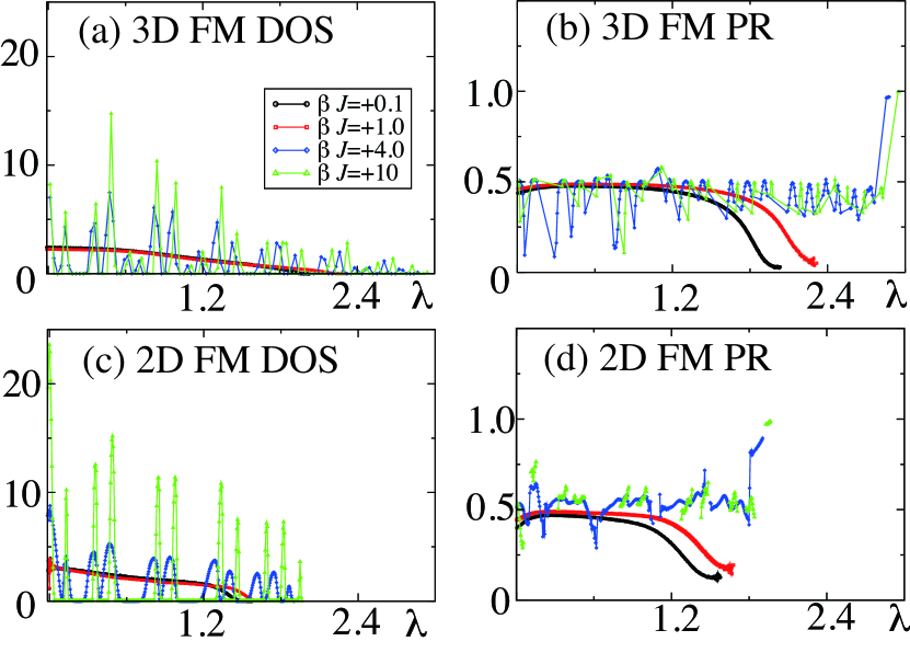
Figure 6: (a) DOS $D(\lambda)$ and (b) PR$(\lambda)$ of the 3D FM system for $L=12$ and $0.1\leq\beta J\leq 10$. $D(\lambda)$ is smooth for $\beta J=0.1,1.0$, whereas it is spiky for $\beta J=4.0,10.0$. For $\beta J=0.1,1.0$, PR$(\lambda)$ decreases as $\lambda$ approaches to the band edges. In contrast, for $\beta J=4.0,10.0$, PR$(\lambda)$ increases sharply near the band edges. (c) DOS $D(\lambda)$ and (d) PR$(\lambda)$ of the 2D FM system for $L=12$ and $0.1\leq\beta J\leq 10$. These quantities exhibit similar behavior with those in the 3D case.

The target system in the FM case ($\beta J>0$) may exhibit qualitatively different behaviors from the AF case because $\langle|Q_{xi}|^{2}\rangle$ increases from 0 to 1 as $\beta J$ varies from $-\infty$ to $\infty$. In Figs. 6 (a),(c), we show FM density of state (DOS), $D(\lambda)$ defined by

$$D(\lambda)=\frac{d\delta}{d\lambda},$$ (6.1)

for $L=12$ and various $\beta J$’s. In Figs. 6 (b),(d), we show the corresponding PR’s.

Let us see the 3D case first. In the $\beta J=0.1$ and $1.0$ cases, which correspond to the PM phase ($0<\beta J\lesssim 1.4$), both $D(\lambda)$ and PR$(\lambda)$ are rather smooth, and PR of Fig. 6 (b) has a similar behavior to PR of Fig. 4 (c) for $\beta J=-0.1$ in the PM phase. However as $\beta J$ increases into the FM phase ($\beta J\gtrsim 1.4$), the FM DOS and PR’s for $\beta J=4.0$ and $10.0$ in Figs. 6 (a),(b) develop spiking structures, while the AF PR for $\beta J=-10.0$ in Fig. 4 (c) remains smooth. This reminds us of the plane wave state of a free fermion with a uniform hopping ($Q_{xi}\to q=|q|e^{i\alpha}$). The energy $\lambda_{\rm\scriptscriptstyle{f}ree}$ and $\phi^{\rm\scriptscriptstyle{f}ree}_{x}$ of a free fermion are given by

$$\lambda_{\rm\scriptscriptstyle{f}ree} = -|q|\sum_{i=1}^{D}\cos(k_{i}+\alpha),\ k_{i}=\frac{2\pi n_{i}}{L},n_{i}=1,\cdots,L,$$

$$\phi^{\rm\scriptscriptstyle{f}ree}_{x} = \frac{1}{\sqrt{L^{D}}}\exp(i\sum_{i}k_{i}x_{i}).$$ (6.2)

$\lambda_{\rm\scriptscriptstyle{f}ree}$ exhibits similar spikes in $D(\lambda)$ in its interval $\lambda_{\rm\scriptscriptstyle{f}ree}=(-D|q|,D|q|)$ and PR$(\lambda)$ = 1. Its origin is just the discreteness of the momentum $k_{i}$.

For sufficiently large $\beta J$, this similarity can be understood as follows; The O(3) model of Eq. (2.12) for $\beta J\gg 1$ forces $|Q_{xi}|\simeq 1$. This implies $Q_{xi}\simeq\exp(i\varphi_{x})\exp(-i\varphi_{x+i})$ for each $z$-sample, and furthermore the phase $\varphi_{x}$ can be absorbed into $\hat{\psi}_{x}$ giving rise to the free fermion system with $q=1$. However, Fig. 6 (b) shows PR $\lesssim 0.5$ instead of PR $\simeq 1$ except for the states in the vicinity of the band edge. This unexpected reduction of PR by factor $\sim 2$ is attributed to the slight deviation $1-\langle|Q_{xi}|^{2}\rangle\neq 0$ for $\beta J<\infty$ [we estimated it as $1-\langle|Q_{xi}|^{2}\rangle\simeq 0.03$ for $\beta J=10.0$]. Although it generates certainly a small change in thermodynamical quantities such as the internal energy, it induces interference effect on the wave function and the energy of fermions in destructive manner. Similar discrepancy is observed in the random-phase hopping model (RPHM) rphm , although the RPHM does not have the local gauge symmetry.

Let us turn to the 2D case. In Fig. 6, we show (c) 2D FM $D(\lambda)$ and (d) 2D FM PR$(\lambda)$ for $L=12$ and various $\beta J$’s. Both the DOS and PR are smooth for smaller $\beta J$ (= 0.1, 1.0) and exhibit a spike structure for larger $\beta J$ (= 4.0, 10.0) as in the 3D case. Explicitly, for all $\beta J$’s, PR$(\lambda)$ keeps $\sim 0.5$ in the central region. For $|\lambda|\gtrsim 0.2$, PR$(\lambda)$ decreases rather sharply for $\beta J=0.1,1.0$, whereas it keeps the similar values and even approaches $\sim 1$ in the vicinity of the band edges for $\beta J=4.0$ and $10.0$. This behavior is quite similar to the 3D $D(\lambda)$ of Fig. 6 (b). We expect that, in the limit $\beta J\to\infty$, the 2D eigenstates converge to the plane-wave states of Eq. (6.2).

These contrasting behaviors (i.e., smooth and spiky) of the 2D and 3D PR$(\lambda)$ near the band edges for two regions of $\beta J$, (1) $\beta J\in(-10.0,+1.0)$ and (2) $\beta J\in(4.0,10.0)$ imply that some critical value $\beta J=(\beta J)_{\rm c}$ exists at which all the states become delocalized, i.e., $\lambda_{\rm\scriptscriptstyle{M}E}=\lambda_{\rm\scriptscriptstyle{M}AX}$. This may be expected as one extends Fig. 5 (a) for $J=-1$ into the positive-$J$ region. This critical point is to be induced because the squared hopping amplitude $|Q_{xi}|^{2}$ runs from 0 to 1 as $\beta J$ runs from $-\infty$ to $\infty$ both for the 2D and 3D systems. The 2D O(3) spin model has no phase transitions in contrast with the 3D model. Therefore the phase transition of the correlated-spin background itself is not a necessary condition for the existence of $(\beta J)_{\rm c}$ itself. Calculation of $(\beta J)_{\rm c}\in(1.0,4.0)$ requires further analyses of PR$(\lambda)$, etc.

VII Conclusion

In summary, we studied the LD of a realistic gauge model of fermions in the correlated spin background by using the conventional techniques for random systems and level statistics. As emphasized in introduction, the strong correlations between the original electrons generate the fluctuating spin background with the correlation of the O(3) model in the present model. We assume that the spin serves as a random quasi-static background controlling the fermion hopping amplitude.

First, we studied the model in 2D and 3D for the AF spin coupling by the ULSD. Finite-size scaling analysis of the ULSD indicates the existence of the ME in the 3D case, whereas it does not give a clear conclusion for the 2D case. Then, we investigated the PR and its finite-size scaling. The results imply that all the states are localized in the 2D case, but more detailed study is required to obtain a clear conclusion. In fact, for some related models of a 2D electron gas in a random magnetic field and an on-site random potential, a Kosterlitz-Thouless-type metal-insulator transition was pointed out xie and also existence of a hidden degree of freedom was suggested nguyen . As the amplitude and phase of the hopping $Q_{xi}$ are both random variables, the model in the present work may have some resemblance with the above ones. This is a future problem. In any case, these methods work well allowing us to calculate the 3D critical temperature $T_{\rm LD}(\delta)$ of the LD transition. It shows that the region of localized states is enhanced in the AF phase. The result of PR for the FM spin coupling indicated some critical point $(\beta J)_{\rm c}$ at which all the states become delocalized ($\lambda_{\rm\scriptscriptstyle{M}E}=\lambda_{\rm\scriptscriptstyle{M}AX}$).

Concerning to the relation between the magnetic phase transition of the O(3) spin model and the LD phase transition, one might expect some strong correlation between them. In fact, our result that a ME exists in the 3D AF case while no clear evidence of ME (probably a crossover) in the 2D AF case is compatible with the fact that the O(3) transition existing in the 3D case disappears in the 2D case. However, we think that this is just accidental coincidence. In fact, Anderson model and related models with uncorrelated randomness show a ME in 3D but not in 2D, which is explained without additional phase transitions. Also our result of Fig. 5(b) shows that the ME generally takes place not on the O(3) transition line. The O(3) spin transition is a thermodynamic transition concerning to a global change in nature of the system, while the LD transition is related with the transport properties, and the details of each eigenstate are an essential ingredient for that. This point shares some common aspect with the discussion at the end of Sec. VI for the critical value at which $\lambda_{\rm\scriptscriptstyle{M}E}=\lambda_{\rm\scriptscriptstyle{M}AX}$.

References

- (1) P. W. Anderson, Phys. Rev., 109, 1492 (1958).
-
(2)
E. Abrahams et al. Phys. Rev. Lett., 42, 673 (1979);
H. Grussbach, M. Schreiber, Phys. Rev. B 51, 663 (1995);
S. Hikami, Phys. Rev. B 24,2671 (1981);
K. B. Effetov, A. I. Larkin, D. E. Khmel’nitsukii, JETP 52, 568 (1980);
K. B. Effetov, ”Supersymmetry in Disorder and Chaos”, Cambridge Univ. Press (1977). -
(3)
H. Fukuyama, J. Phys. Soc. Jpn., 50, 3652 (1981);
C. Castellani, C. Di. Castro, P. A. Lee, and M. Ma,
Phys. Rev. B 30, 527 (1984). -
(4)
A. Smith, J. Knolle, D. L. Kovrizhin, and R. Moessner,
Phys. Rev. Lett. 118, 266601 (2017);
A. Smith, J. Knolle, R. Moessner, and D. L. Kovrizhin,
Phys. Rev. Lett. 119, 176601 (2017). -
(5)
T. G. Kovács and F. Pittler, Phys. Rev. Lett. 105, 192001 (2010);
S. M. Nishigaki, M. Giordano, T. G. Kovács, and
F. Pittler, https://pos.sissa.it/187/018/pdf;
L. Ujfalusi, M. Giordano, F. Pittler, T. G. Kovács, and
I. Varga, Phys. Rev. D 92, 094513 (2015). - (6) A. Kitaev, Ann. Phys. 321, 2 (2006).
-
(7)
A. Smith, J. Knolle, R. Moessner, and D. L. Kovrizhin,
Phys. Rev. B 97, 245137 (2018). -
(8)
P. W. Anderson, Science 235, 1196(1987);
P. W. Anderson, G. Baskaran, Z. Zou and T. Hsu, Phys. Rev. Lett. 58, 2790(1987);
A. E. Ruckenstein, P. J. Hirschfeld and J. Appel, Phys. Rev. B 36, 857(1987);
G. Baskaran, Z. Zou and P. W. Anderson, Solid State Comm. 63, 973(1987). - (9) G. Kotliar and A. Ruckenstein, Phys. Rev. Lett. 57, 2790 (1987).
- (10) I. Ichinose and T. Matsui, Phys. Rev. B 45, 9976 (1992).
-
(11)
For the cubic lattice,
extended states disappear, i.e., as
from below.
See A. Mac Kinnon and B. Kramer, Phys. Rev. Lett. 47, 1546
(1981);
Z. Phys. B 53, 1 (1983), B. Kramer, A. Mac Kinnon, and M. Shreiber, Physica A 167, 163 (1990). - (12) The complex projective space CPN-1 is defined as . This equivalence class is incorporated by the U(1) local gauge invariance. For , with , CP.
- (13) The case of moderate doping is discussed comprehensively in Ref. sf .
- (14) In of Eq. (2.12), we flipped the signature of from the AF spin coupling of the - model (2.6).
- (15) M. Schiulaz and M. Muller, AIP Conf. Proc. 1610, 11 (2014).
- (16) N. Y. Yao, C. R. Laumann, J. I. Cirac, M. D. Lukin, and J. E. Moore, Phys. Rev. Lett. 117, 240601 (2016).
- (17) The electron operator in Eq. (2.6) is also invariant under the corresponding local gauge transformation,
- (18) The value is chosen so that the difference between two intermediate integrals of ULSD, , for the Poisson type and the Wigner type () in Eq. (3.3) becomes maximum.
-
(19)
B.I. Shklovskii, B. Shapiro, B.R. Sears, P. Lambrianides
and H.B. Shore, Phys. Rev. B 47, 11487(1993);
E. Hofstetter, Phys. Rev. B 57, 12763(1998). -
(20)
M. Giordano, T. G. Kovács, and F. Pittler, Phys. Rev. Lett. 112, 102002 (2014);
T. G. Kovács and R. A. Vig, Phys. Rev. D 97, 014502 (2018). - (21) Both in the 2D and 3D cases, exceeds for some ’s, which implies that there favors localized states more than the Poisson type.
- (22) A Rodriguez, L. J. Vasquez, K. Slevin, and R. A. Römer, Phys. Rev. Lett. 105, 046403 (2010).
- (23) If such regions with each volume are assembled quasiperiodically and superposed to make a Bloch-type delocalized state, and .
- (24) P. A. Lee, N. Nagaosa, and X. G. Wen, Rev. Mod. Phys. 78, 17 (2006).
-
(25)
H. Yamamoto, G. Tatara, I. Ichinose and T. Matsui, Phys. Rev. B 44, 7654 (1991);
I. Ichinose and T. Matsui, Phys. Rev. B 51, 11860 (1995). -
(26)
The random phase hopping model is defined by replacing
of Eq. (2.2) by a random phase factor with the unit magnitude,
, where is a uniformly distributed
random angle independently defined link by link.
T. Ohthuki, Y. Ono, and B. Kramer, J. Phys. Soc. Jpn. 63, 685 (1994);
For the 2D model, see T. Sugiyama and N. Nagaoka, Phys. Rev. Lett 70, 1980 (1993);
C. Pryor and A. Zee, Phys. Rev. B 46, 3116 (1992);
Y. Avishai, Y. Hatsugai and M. Kohmoto, Phys. Rev. B47, 9561 (1993);
V. Kalmeyer, D. Wei, D. P. Arovas, and S. C. Zhang, Phys. Rev. B48, 11095 (1993). - (27) X. C. Xie, X. R. Wang, and D. Z. Liu, Phys. Rev. Lett. 80, 3563 (1998).
- (28) H. K. Nguyen, Phys. Rev. B 66, 144201 (2002).