Flows, Fixed Points and Duality in Chern-Simons-matter theories

Abstract

It has been conjectured that 3d fermions minimally coupled to Chern-Simons gauge fields are dual to 3d critical scalars, also minimally coupled to Chern-Simons gauge fields. The large $\displaystyle N$ arguments for this duality can formally be used to show that Chern-Simons-gauged critical (Gross-Neveu) fermions are also dual to gauged ‘regular’ scalars at every order in a $\displaystyle 1/N$ expansion, provided both theories are well-defined (when one fine-tunes the two relevant parameters of each of these theories to zero). In the strict large $\displaystyle N$ limit these ‘quasi-bosonic’ theories appear as fixed lines parameterized by $\displaystyle x_{6}$, the coefficient of a sextic term in the potential. While $\displaystyle x_{6}$ is an exactly marginal deformation at leading order in large $\displaystyle N$, it develops a non-trivial $\displaystyle\beta$ function at first subleading order in $\displaystyle 1/N$. We demonstrate that the beta function is a cubic polynomial in $\displaystyle x_{6}$ at this order in $\displaystyle 1/N$, and compute the coefficients of the cubic and quadratic terms as a function of the ’t Hooft coupling. We conjecture that flows governed by this leading large $\displaystyle N$ beta function have three fixed points for $\displaystyle x_{6}$ at every non-zero value of the ’t Hooft coupling, implying the existence of three distinct regular bosonic and three distinct dual critical fermionic conformal fixed points, at every value of the ’t Hooft coupling. We analyze the phase structure of these fixed point theories at zero temperature. We also construct dual pairs of large $\displaystyle N$ fine-tuned renormalization group flows from supersymmetric $\displaystyle{\cal N}=2$ Chern-Simons-matter theories, such that one of the flows ends up in the IR at a regular boson theory while its dual partner flows to a critical fermion theory. This construction suggests that the duality between these theories persists at finite $\displaystyle N$, at least when $\displaystyle N$ is large.

1 Introduction and summary

This paper is devoted to the study of a web of five closely related classes of Chern-Simons-matter theories, with gauge groups $\displaystyle SO(N)$, $\displaystyle SU(N)$ or $\displaystyle U(N)$ and matter in the fundamental representation. The five classes of three dimensional quantum field theories that we study include several conformal field theories. More general theories are obtained by deforming these fixed points with relevant operators. Distinct theories in this web are related by renormalization group flows and by quantum-corrected Legendre transformations at large $\displaystyle N$. Less trivially, several distinct theories that we study are also conjectured to be related to each other by strong-weak coupling dualities that exchange bosons and fermions.

There are many reasons to be interested in Chern-Simons-matter theories of the type studied in this paper. Despite the fact that they are effectively solvable in the large $\displaystyle N$ limit, these theories are dynamically very rich and display properties that are unusual for quantum field theories. As already mentioned, these theories enjoy invariance under strong-weak coupling bosonization dualities even in the absence of supersymmetry. Moreover, both S matrices and thermal partition functions of these theories have very unusual properties, including modified transformations under crossing symmetry of the S matrix (see below for references). The effective solvability of these models at large $\displaystyle N$ permits the detailed study of these interesting phenomena. It is possible that the lessons learned from this study will apply more generally to all Chern-Simons-matter theories, even away from the large $\displaystyle N$ limit.

The next set of motivations for the study of these theories comes from the AdS/CFT correspondence. The theories we study have been suggested Klebanov:2002ja ; Sezgin:2002rt ; Giombi:2009wh ; Giombi:2011kc ; Chang:2012kt to have another dual description at large $\displaystyle N$, in terms of theories of classical high-spin gravity on $\displaystyle AdS_{4}$ (see Giombi:2016ejx and references therein). While this duality is precise only in the strict large $\displaystyle N$ limit, the field theories are well-defined even at finite $\displaystyle N$, and provide the only known quantization of the bulk dual higher spin theories.

Next, there are many known results for highly supersymmetric cousins of these theories, including conjectured field theory dualities and also conjectured dualities of some of these theories at strong coupling to bulk supergravity, string theory or M theory Aharony:2008ug . The combination of the large $\displaystyle N$ techniques used in this paper with the exact results from supersymmetry could lead to unanticipated synergies.

Yet another set of motivations for the study of the theories considered in this paper comes from condensed matter physics. Finite $\displaystyle N$ versions of the theories studied herein have already found applications in condensed matter physics in the study of the quantum Hall effect (see below for some references). It does not seem implausible that more such applications will be found over the coming years.

This self-contained introductory section is divided into two subsections. In subsection 1.1 we introduce the Chern-Simons-matter theories studied in this paper and present a brief summary of known results about these theories. In subsection 1.2 we summarize the main results of this paper.

1.1 The theories we study

1.1.1 Listing of theories

The five classes of theories of interest to this paper are the following $\displaystyle U(N)$ gauge theories :

• The $\displaystyle{\cal N}=2$ supersymmetric (S) Chern-Simons-matter theory with a single chiral multiplet in the fundamental representation:

  $$\displaystyle S_{S}(\phi,\psi) \displaystyle=\int d^{3}x\biggl{[}i\varepsilon^{\mu\nu\rho}\frac{\kappa}{4\pi}\mathrm{Tr}(A_{\mu}\partial_{\nu}A_{\rho}-\frac{2i}{3}A_{\mu}A_{\nu}A_{\rho})+D_{\mu}\bar{\phi}D^{\mu}\phi+\bar{\psi}\gamma^{\mu}D_{\mu}\psi$$

  $$\displaystyle\qquad\qquad\qquad+\frac{4\pi^{2}}{\kappa^{2}}(\bar{\phi}\phi)^{3}+\frac{4\pi}{\kappa}(\bar{\psi}\psi)(\bar{\phi}\phi)+\frac{2\pi}{\kappa}(\bar{\psi}\phi)(\bar{\phi}\psi)\biggl{]}.$$ (1)

• The critical bosonic (CB) theory (the critical $\displaystyle U(N)$ model coupled to a Chern-Simons (CS) gauge field):

  $$S_{CB}(\phi,\sigma_{B})=\int d^{3}x\biggl{[}i\varepsilon^{\mu\nu\rho}\frac{\kappa_{B}}{4\pi}\mathrm{Tr}(A_{\mu}\partial_{\nu}A_{\rho}-{2i\over 3}A_{\mu}A_{\nu}A_{\rho})+D_{\mu}\bar{\phi}D^{\mu}\phi+\sigma_{B}\bar{\phi}\phi\biggl{]}.$$ (2)

• The regular fermion (RF) theory (fermions coupled to a CS gauge field):

  $$S_{RF}(\psi)=\int d^{3}x\bigg{[}i\varepsilon^{\mu\nu\rho}{\kappa_{F}\over 4\pi}\mathrm{Tr}(A_{\mu}\partial_{\nu}A_{\rho}-{2i\over 3}A_{\mu}A_{\nu}A_{\rho})+\bar{\psi}\gamma_{\mu}D^{\mu}\psi\bigg{]}.$$ (3)

• The regular boson (RB) theory (scalars coupled to a CS gauge field):

  $$S_{RB}(\phi)=\int d^{3}x\biggl{[}i\varepsilon^{\mu\nu\rho}{\kappa_{B}\over 4\pi}\mathrm{Tr}(A_{\mu}\partial_{\nu}A_{\rho}-{2i\over 3}A_{\mu}A_{\nu}A_{\rho})+D_{\mu}\bar{\phi}D^{\mu}\phi+\frac{(2\pi)^{2}}{\kappa_{B}^{2}}\left(x^{B}_{6}+1\right)(\bar{\phi}\phi)^{3}\biggl{]}.$$ (4)

• The critical fermion (CF) theory (the Gross-Neveu model coupled to a CS gauge field):

  $$S_{CF}(\psi,\sigma_{F})=\int d^{3}x\bigg{[}i\varepsilon^{\mu\nu\rho}{\kappa_{F}\over 4\pi}\mathrm{Tr}(A_{\mu}\partial_{\nu}A_{\rho}-{2i\over 3}A_{\mu}A_{\nu}A_{\rho})+\bar{\psi}\gamma_{\mu}D^{\mu}\psi-\frac{4\pi}{\kappa_{F}}\zeta\bar{\psi}\psi+\frac{(2\pi)^{2}}{\kappa_{F}^{2}}x^{F}_{6}\zeta^{3}\bigg{]}.$$ (5)

The RF and CB theories were together called ‘quasi-fermionic’ theories in Maldacena:2011jn ; Maldacena:2012sf while the RB and CF theories were referred to as ‘quasi-bosonic’ theories. We will employ this nomenclature in the rest of this paper.

In the rest of this subsection we briefly review the definition and key properties of the five classes of theories listed above.

1.1.2 Supersymmetric theories S

The supersymmetric (SUSY) theories S are quite well understood. The Lagrangian (1) (in the dimensional reduction regulation scheme) is known to define a superconformal fixed point Gaiotto:2007qi with four supercharges. At least at weak coupling, this fixed point has three relevant and no marginal deformations.

These superconformal fixed points are conjectured Benini:2011mf ; Park:2013wta ; Aharony:2013dha to enjoy invariance under a strong-weak coupling self-duality similar to the Giveon-Kutasov duality Giveon:2008zn (see appendix E for some details). This duality reshuffles bosons and fermions within supermultiplets Jain:2013gza ; Inbasekar:2015tsa ; Gur-Ari:2015pca , and so can be thought of as a bosonization duality. There is considerable evidence that this duality holds for all values of $\displaystyle N$ and $\displaystyle\kappa$ for which the theory has a supersymmetric vacuum. The evidence for this duality includes several calculational checks using the method of supersymmetric localization Kapustin:2010mh ; Willett:2011gp ; Kapustin:2011gh , as well as the relation of this duality by flows to many other supersymmetric dualities (see, for instance, Intriligator:2013lca ; Aharony:2013dha ).

1.1.3 Quasi-Fermionic theories

The critical boson and regular fermion theories are also relatively well understood. The CB theory may be thought of as the $\displaystyle U(N)$ Wilson-Fisher theory gauged by a Chern-Simons gauge field. The RF theory is even simpler; it may be thought of as a collection of $\displaystyle N$ free complex fermions minimally coupled to a $\displaystyle U(N)$ Chern-Simons gauge field. Neither of the Lagrangians (5) or (3) has a continuous dimensionless parameter. It follows that the path integrals with these Lagrangians define isolated conformal field theories (in dimensional reduction regulation schemes) Aharony:2011jz ; Giombi:2011kc whenever they are well-defined. The resultant conformal theories both have a single relevant deformation - a mass term for the bosons or fermions respectively.

The theories CB and RF – the so called ‘quasi-fermionic theories’ – have been conjectured to be related to each other via a strong weak coupling duality that exchanges (2) and (3). The existence of such a duality was first suggested in Giombi:2011kc ; the first concrete conjecture for this duality was made in Aharony:2012nh based partly on the results of Maldacena:2011jn ; Maldacena:2012sf . See Aharony:2015mjs for a recent and relatively precise statement of the conjectured dualities, and Seiberg:2016gmd for an even more precise version.

Below we review a proposed ‘derivation’ of this duality. Here we merely note that there exists substantial independent calculational evidence for the conjectured duality between theories CB and RF in the ’t Hooft large $\displaystyle N$ limit $\displaystyle N\to\infty$, $\displaystyle\kappa\to\infty$ with the ’t Hooft coupling $\displaystyle\lambda=N/\kappa$ held fixed. In this limit these theories all have high-spin symmetries which severely constrain their dynamics Maldacena:2011jn ; Maldacena:2012sf . The evidence for duality includes the matching of correlators Aharony:2012nh ; GurAri:2012is ; Bedhotiya:2015uga , S matrices Jain:2014nza ; Dandekar:2014era ; Yokoyama:2016sbx and thermal partition functions Giombi:2011kc ; Jain:2012qi ; Aharony:2012ns ; Jain:2013py ; Takimi:2013zca ; Yokoyama:2013pxa ; Yokoyama:2012fa on the two sides of the duality. Independent evidence for these dualities at large but finite $\displaystyle N$ includes the matching of part of the baryon and monopole spectra between these theories Radicevic:2015yla ; Aharony:2015mjs . There is also some evidence that these dualities continue to hold at small values of $\displaystyle N$; in particular at specific small values of $\displaystyle N$ and $\displaystyle\kappa$ they may be related to independently conjectured dualities that show up in condensed matter systems Seiberg:2016gmd ; Karch:2016sxi .

The CB and RF theories, and the conjectured duality between them, are reviewed in more detail in section 2 below.

1.1.4 A ‘derivation’ of quasi-fermionic dualities from SUSY dualities

In this subsubsection we review the ‘derivation’ Jain:2013gza ; Gur-Ari:2015pca of the duality between the quasi-fermionic theories CB and RF starting from the assumed self-duality of the supersymmetric theories S.

As mentioned above, the supersymmmetric theory S admits at least 3 relevant deformations at large $\displaystyle N$. It follows that there exists an (at least) 2 parameter set of renormalization group (RG) flows originating at this theory. The self-duality of theory S identifies pairs of naively different RG flows.

The authors of Jain:2013gza identified a one parameter tuning of the large $\displaystyle N$ flows that originate at S, with the property that all these flows end up in the IR at the critical boson theory CB. They then demonstrated that the duals to these flows all end up at the regular fermion theory RF. At large $\displaystyle N$ the duality of the CB and RF theories thus follows as a consequence of the duality of theory S.

Now consider two flows: the infinite $\displaystyle N$ flow $\displaystyle F$ of Jain:2013gza ; Gur-Ari:2015pca and a large but finite $\displaystyle N$ flow $\displaystyle F^{\prime}$ that coincides with $\displaystyle F$ in the deep UV. As the $\displaystyle\beta$ functions that govern $\displaystyle F^{\prime}$ differ only slightly from the $\displaystyle\beta$ functions that govern $\displaystyle F$, the two flows will deviate only slightly from each other over RG flow ‘times’ that are independent of $\displaystyle N$. It follows that the flow $\displaystyle F^{\prime}$ will approach very near to the quasi-fermion fixed point, before eventually being repelled away from it along the direction of its relevant operator. However any flow that approaches a neighborhood of the IR fixed point can generically be retuned to ensure that it actually ends up precisely at the fixed point, provided the number of parameters characterizing the UV RG flows (in this case 2) is greater than or equal to the number of relevant operators about the IR fixed point (in this case 1). These considerations suggest that the duality between the CB and RF theories continues to hold for finite large values of $\displaystyle N$. It may hold also for smaller values.

1.1.5 Quasi-Bosonic theories

We now turn to the theories that are the main focus of our paper, namely the regular boson and critical fermion theories. These theories are harder to define than their quasi-fermionic counterparts. In order to explain why this is the case, we first review the situation with the simplest of these theories, the regular boson theory at $\displaystyle\kappa_{B}=\infty$, i.e. $\displaystyle\lambda_{B}=0$. To keep the action (4) finite we need to define a new coupling $\displaystyle\lambda_{6}=x_{6}^{B}\lambda_{B}^{2}$ which remains finite as $\displaystyle\lambda_{B}\to 0$. In this special case the Lagrangian (4) is free when the classically marginal parameter $\displaystyle\lambda_{6}=0$, and the two relevant operators $\displaystyle|\phi|^{2}$ and $\displaystyle|\phi|^{4}$ are tuned to zero. It is no longer free at $\displaystyle\lambda_{6}\neq 0$. A one-loop computation (see e.g. Pisarski:1982vz ) establishes that the deformation about the free theory parameterized by $\displaystyle\lambda_{6}$, while classically marginal, is actually marginally irrelevant at positive values of $\displaystyle\lambda_{6}$ . It follows that the theories at positive $\displaystyle\lambda_{6}$ cannot be defined by renormalization group flows away from the free theory, and have no obvious definition.

The situation is, however, better in the large $\displaystyle N$ limit. The $\displaystyle\beta$ function of this theory (still at $\displaystyle\kappa_{B}=\infty$) was computed by Pisarski at first non-trivial order at large $\displaystyle N$ but at all values of $\displaystyle\lambda_{6}$, and turns out Pisarski:1982vz to take the form

$$\beta_{\lambda_{6}}=\frac{1}{N}\left(a(\lambda_{6})^{2}-b(\lambda_{6})^{3}\right)+{\cal O}(1/N^{2}),$$ (6)

where $\displaystyle a$ and $\displaystyle b$ are known positive constants of order unity. In addition to $\displaystyle\lambda_{6}=0$, the $\displaystyle\beta$ function (6) vanishes at $\displaystyle\lambda_{6}=\frac{a}{b}$. Moreover the operator $\displaystyle|\phi|^{6}$ is relevant about this new fixed point. RG flows that originate in this fixed point define the $\displaystyle\kappa_{B}=\infty$ large $\displaystyle N$ RB theory at every positive value of $\displaystyle\lambda_{6}$. As the $\displaystyle\beta$ function of the theory at finite but large values of $\displaystyle N$ deviates only slightly from (6) at values of $\displaystyle\lambda_{6}$ that are of order unity, it follows that this fixed point continues to exist, continues to be repulsive and continues to define the $\displaystyle\kappa_{B}=\infty$ RB theory at finite but large $\displaystyle N$ .

In this paper (see the next subsection for more details) we compute the generalization of the leading large $\displaystyle N$ beta function (6) to non-zero $\displaystyle\lambda_{B}$, and thereby provide a definition of the RB theories at finite but large values of $\displaystyle N$ and $\displaystyle\kappa_{B}$ .

We now turn to the second quasi-bosonic theory, namely the critical fermion theory. In this case the theory (5) has no obvious free point. To the best of our knowledge, the RG flows of $\displaystyle x_{6}^{F}$ in this model have not previously been studied at any value of $\displaystyle N$ or $\displaystyle\kappa_{F}$, not even in the effectively ungauged limit $\displaystyle\kappa_{F}\rightarrow\infty$. In this paper we compute the $\displaystyle\beta$ function for $\displaystyle x_{6}^{F}$ in the large $\displaystyle N$ limit, and use the results of our computation to propose a definition for the CF theories at all values of $\displaystyle\lambda_{F}$, even at finite (but large) values of $\displaystyle N$. Note that the results of our paper also give a precise definition of the large $\displaystyle N$ ungauged $\displaystyle 3d$ Gross-Neveu model.

1.2 The principal results of this paper

The principal new results of this paper are a computation of the leading large $\displaystyle N$ beta functions of the two quasi-bosonic theories, an analysis of their large $\displaystyle N$ zero temperature phase structure, and the construction of dual pairs of RG flows from the $\displaystyle{\cal N}=2$ superconformal fixed points to the two different quasi-bosonic theories, supporting the conjectured existence and duality of these theories. In this subsection we review each of these results in turn. We discuss in this paper only the special case of a single matter field.

1.2.1 Beta functions for quasi-bosonic theories

In this paper we analyze the leading large $\displaystyle N$ $\displaystyle\beta$ functions of $\displaystyle x_{6}$ in the two quasi-bosonic theories. We show that for all values of the ’t Hooft coupling these beta functions are third-order polynomials in $\displaystyle x_{6}$, and we explicitly compute the coefficient of $\displaystyle x_{6}^{3}$. This is enough to understand the qualitative form of the renormalization group flows. The lower coefficients are known perturbatively, but not for all values of the ’t Hooft coupling. One way to compute these coefficients more generally is by computing and summing the infinite number of leading non-planar Feynman diagrams in the quasi-bosonic theories that contribute to this beta function. Instead of doing this explicitly, we relate these coefficients to computations in the quasi-fermionic theories.

As we explain in detail below (see around (102)), each quasi-bosonic theory may be viewed as a (quantum) Legendre transform of its quasi-fermionic counterpart. The Legendre transform is taken with respect to the lowest dimension scalar operator $\displaystyle J_{0}$ of the corresponding quasi-fermionic theory. Schematically

$$\begin{split}Z_{\rm{reg~{}boson}}&=\int D\zeta<e^{\int\zeta J_{0}+x_{6}\zeta^{3}}>_{\rm{crit~{}boson}}\\ Z_{\rm{crit~{}fermion}}&=\int D\zeta<e^{\int\zeta J_{0}+x_{6}\zeta^{3}}>_{\rm{reg~{}fermion}}\\ \end{split}$$ (7)

(see (94) and (97) for non-cartoon versions of these equations).

In order to evaluate the quasi-bosonic partition functions on the left-hand side of (7) we first evaluate the expectation values in the integrand of the right-hand side. The result is an effective action for $\displaystyle\zeta$ whose $\displaystyle n^{th}$ order vertices are the $\displaystyle n$-point Green’s functions of $\displaystyle J_{0}$ in the corresponding quasi-fermionic theory. This effective action is less formal than it might first seem, as its leading terms, related to the two, three and four point functions of $\displaystyle J_{0}$, are explicitly known at all values of $\displaystyle\lambda$ in the large $\displaystyle N$ limit, as we review in some detail below.

Note that the leading large $\displaystyle N$ effective action for $\displaystyle\zeta$ comes from integrating out $\displaystyle N$ fundamental fields, and so it is (in a natural normalization) proportional to $\displaystyle N$. Note also that the correlators of $\displaystyle J_{0}$ of the two different quasi-fermionic theories are already known (or conjectured) to map to each other under duality, so the effective actions (7) for $\displaystyle\zeta$ are automatically duality-covariant.

At the next step in the computation of our $\displaystyle\beta$ function, we perform the path integral over the Lagrange multiplier fields $\displaystyle\zeta$. As the action for the Lagrange multiplier fields has an overall factor of $\displaystyle N$, the leading large $\displaystyle N$ contribution to the $\displaystyle\beta$ function is given only by one loop graphs from this effective action (see Pomoni:2008de for a similar observation in a different context). This is true at all values of $\displaystyle\lambda$ and $\displaystyle x_{6}^{B}$ (or $\displaystyle x_{6}^{F}$). Evaluating the divergent pieces of these one loop graphs we find that the $\displaystyle\beta$ function for $\displaystyle x_{6}=x_{6}^{B}=x_{6}^{F}$, for flows towards the UV, is given by

$$\begin{split}&\frac{dx_{6}}{d\ln(\Lambda)}=-a+bg_{3}-cg_{3}^{3},\\ &g_{3}\equiv 24\pi^{2}\left(x_{6}-\frac{4}{3}\cot^{2}\left(\frac{\pi\lambda_{B}}{2}\right)\right)=24\pi^{2}\left(x_{6}-\frac{4}{3}\tan^{2}\left(\frac{\pi\lambda_{F}}{2}\right)\right).\\ \end{split}$$ (8)

Note in particular that $\displaystyle g_{3}$ is linearly related to $\displaystyle x_{6}$, and so the $\displaystyle\beta$ function in (8) is a cubic function of $\displaystyle x_{6}$ at every value of $\displaystyle\lambda_{B}$ and $\displaystyle\lambda_{F}$, the ’t Hooft couplings of the RB and CF theories, respectively. Here

$$\begin{split}c&=\frac{1}{24\pi^{2}}\left(\frac{1}{2\pi^{2}\kappa_{B}g_{2}^{3}}\right),\\ g_{2}&\equiv\left(\frac{4\pi}{\tan(\frac{\pi\lambda_{B}}{2})}\right)=-\left(\frac{4\pi}{\cot(\frac{\pi\lambda_{F}}{2})}\right),\\ \kappa_{B}&=-\kappa_{F},~{}~{}~{}~{}\lambda_{B}=\lambda_{F}-{\rm sgn}(\lambda_{F}).\\ \end{split}$$ (9)

Note that $\displaystyle c$ is positive for all values of $\displaystyle\lambda_{B}$ and $\displaystyle\lambda_{F}$ (ranging from $\displaystyle(-1)$ to $\displaystyle 1$).

Like $\displaystyle c$, the coefficients $\displaystyle a$ and $\displaystyle b$ are functions of $\displaystyle\lambda_{B}$ and $\displaystyle\lambda_{F}$, and are of order $\displaystyle 1/N$, but they are independent of $\displaystyle x_{6}$. $\displaystyle a$ and $\displaystyle b$ are determined (see (132)) in terms of coefficients that characterize particular kinematical limits of the leading large $\displaystyle N$ 3-, 4-, and 5-point functions of the operator $\displaystyle J_{0}$ in the quasi-fermionic theories, together with two numbers that require a subleading-in-$\displaystyle 1/N$ computation : the first correction to the anomalous dimension of $\displaystyle J_{0}$ in these theories, and the coefficient governing the splitting of the 3-point function (once this anomalous dimension is non-zero) into a contact term and a non-contact term. The leading large $\displaystyle N$ three and four-point functions are known exactly. However the leading large $\displaystyle N$ five-point function and the two sub-leading $\displaystyle 1/N$ corrections referred to above are currently known only at small $\displaystyle\lambda_{B}$ or small $\displaystyle\lambda_{F}$. Practically speaking, therefore, $\displaystyle a$ and $\displaystyle b$ are currently known only at small $\displaystyle\lambda_{B}$ or $\displaystyle\lambda_{F}$.

As $\displaystyle c$ is positive, the beta function (8) is negative at large positive values of $\displaystyle x_{6}$ but is positive at large negative values of $\displaystyle x_{6}$ (this is true at every value of $\displaystyle\lambda$). In other words, flows towards the IR drive large positive values of $\displaystyle x_{6}$ to $\displaystyle\infty$ and large negative values of $\displaystyle x_{6}$ to $\displaystyle-\infty$. It follows immediately that our cubic beta function generically has either one unstable fixed point or two unstable and one stable fixed points. The explicit values of $\displaystyle a$ and $\displaystyle b$ at weak bosonic and fermionic coupling suggest – and we conjecture – that the $\displaystyle\beta$ function in fact has three zeroes at every non-zero $\displaystyle\lambda_{B}$. Ordering the fixed points along the $\displaystyle x_{6}$ axis, the first and third of these fixed points are repulsive (for flows towards the IR) while the second fixed point is attractive.

The structure of these RG flows of $\displaystyle x_{6}$ is depicted in Figure 1, where $\displaystyle x_{6}$ labels the horizontal direction. We have added in this figure also the expected behaviour of the quasi-bosonic theories when we turn on their second-most-relevant deformation (a $\displaystyle({\bar{\phi}}\phi)^{2}$ term in (4)), whose coefficient labels the vertical axis, but still tune the most relevant operator to zero. We will discuss this further in section 4.

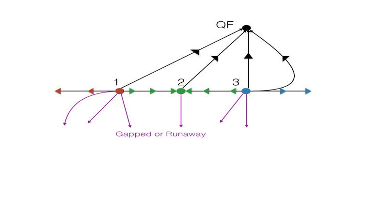
Figure 1: Renormalization group flows of the quasi-bosonic theories as a function of $\displaystyle x_{6}$ (the horizontal axis) and of their second-most-relevant deformation (the vertical axis), when the most relevant operator is fine-tuned to zero.

Note that the second fixed point has a total of $\displaystyle 2$ relevant operators (the mass term and $\displaystyle({\bar{\phi}}\phi)^{2}$) while the other two fixed points have $\displaystyle 3$ relevant operators; the additional operator is parametrized by $\displaystyle x_{6}$.

The $\displaystyle\beta$ function (8) manifestly respects duality invariance: the beta function of the regular boson theory agrees with the beta function of the critical fermion theory under the standard bosonization duality map (see below for more details). As noted above, this feature is built in to our method of computation; it is a direct consequence of the duality covariance of the effective action for the Lagrange multiplier $\displaystyle\zeta$.

Our results allow us to give a clear definition of the space of quasi-bosonic theories, at finite (but large enough) values of $\displaystyle N$. These theories are defined by the space of RG flows away from the two repulsive fixed points .

1.2.2 Phase structure and stability of quasi-bosonic theories

In the ’t Hooft large $\displaystyle N$ limit the $\displaystyle\beta$ function (8) is of order $\displaystyle\frac{1}{N_{B}}$. If we restrict our attention to the large $\displaystyle N_{B}$ limit, the quasi-bosonic theories are thus conformal at every value of $\displaystyle x_{6}$.

At leading order in the large $\displaystyle N_{B}$ limit, the free energy of the quasi-bosonic theories at a finite temperature $\displaystyle T$ has been studied at every value of $\displaystyle x_{6}$ Aharony:2012ns ; Minwalla:2015sca . At the ‘conformal’ point (i.e. at arbitrary $\displaystyle x_{6}$ but with all relevant deformations turned off) the free energy is proportional to $\displaystyle T^{3}$ as expected from conformal invariance. When relevant deformations (masses and $\displaystyle\phi^{4}$ couplings) are turned on, candidate phases are given by solutions to a known set of gap equations (see e.g. Minwalla:2015sca ). These gap equations typically have multiple solutions at any particular value of the microscopic parameters and the temperature. The dominant phase is the solution with the lowest free energy. As microscopic parameters are varied, this dominant phase changes, giving rise to an intricate phase diagram.

The gap equations of the quasi-bosonic theories continue to admit multiple solutions even at zero temperature, though they simplify greatly in this limit. In section 4 below we compute the phase diagram of the RB theory at zero temperature by comparing the free energies of the various solutions to the gap equation. Our final results are graphically summarized in the phase diagrams in Figures 7, 8, and 9 below.

The phase diagram of the RB theory changes as we change $\displaystyle x_{6}$. Interestingly, our final results are qualitatively different depending on whether $\displaystyle x_{6}<\phi_{1}$, $\displaystyle\phi_{1}<x_{6}<\phi_{2}$ or $\displaystyle x_{6}>\phi_{2}$, where $\displaystyle\phi_{1}$ and $\displaystyle\phi_{2}$ are critical values of $\displaystyle x_{6}$ given by

$$\phi_{1}\equiv\frac{4}{3}\left(\frac{1}{(2-|\lambda_{B}|)^{2}}-1\right),\qquad\qquad\phi_{2}\equiv\frac{4}{3}\left(\frac{1}{{\lambda}_{B}^{2}}-1\right).$$ (10)

The upcoming paper new explains this fact by computing an exact Landau Ginzburg potential for the variable $\displaystyle{\bar{\phi}}\phi$ in the RB theory. The phase diagram of the RB theory is obtained by finding all the extrema of this Landau Ginzburg potential and choosing the extremum with the minimum free energy. The differences in the phase structure of the RB theory in different intervals of $\displaystyle x_{6}$ is a consequence of the fact that this Landau Ginzburg potential is qualitatively different in the three regions mentioned above. In particular the Landau Ginzburg potential of new has the property that it is unbounded from below when either $\displaystyle x_{6}<\phi_{1}$ or $\displaystyle x_{6}>\phi_{2}$. When $\displaystyle x_{6}$ lies between $\displaystyle\phi_{1}$ and $\displaystyle\phi_{2}$, on the other hand, the exact Landau Ginzburg potential is bounded below.

The fact that the Landau Ginzburg action is unbounded from below when $\displaystyle x_{6}<\phi_{1}$ or $\displaystyle x_{6}>\phi_{2}$ suggests that the RB theory is unstable in this range of parameters. On the other hand the theory appears to be perfectly stable in the range

$$\phi_{1}<x_{6}<\phi_{2}.$$

Once we take finite $\displaystyle N$ effects into account, we have already seen that the RB theory is really well-defined only at the three fixed points of the $\displaystyle\beta$ function. The relationship of these three fixed point values to $\displaystyle\phi_{1}$ and $\displaystyle\phi_{2}$ is graphically demonstrated in Figure 10, both at weak bosonic coupling and at weak fermionic coupling. Interestingly, the ‘middle’ fixed point of the $\displaystyle\beta$ function (the stable fixed point about which $\displaystyle x_{6}$ is an irrelevant deformation) lies between $\displaystyle\phi_{1}$ and $\displaystyle\phi_{2}$ at both weak bosonic and weak fermionic coupling. We conjecture that this continues to be the case at every value of $\displaystyle\lambda_{B}$, so that this fixed point is always well-defined with a stable vacuum.

1.2.3 Flows from theory S to quasi-bosonic theories

Above we discussed the RG flows of the parameter $\displaystyle x_{6}$ within the manifold of quasi-bosonic theories. In this subsubsection we turn our attention to a different class of flows: flows from the supersymmetric theory S to the manifold of quasi-bosonic theories. The flows that we study in this section are non-trivial even at leading order in the large $\displaystyle N$ limit (unlike the $\displaystyle\beta$ functions of the previous subsubsection that were of order $\displaystyle\frac{1}{N}$), so they are ‘fast’ flows in contrast to the ‘slow’ flows of $\displaystyle x_{6}$ described above. At the end of the current section we will discuss the relationship between these two different classes of flows.

In subsection 1.1.4 we reviewed the one parameter fine-tuning Jain:2013gza ; Gur-Ari:2015pca of the two parameter class of dual pairs of RG flows starting at theory S, that end up in the deep IR in the CB and RF fixed points, respectively. While the discussion of Jain:2013gza ; Gur-Ari:2015pca is correct at generic parameters of the flows, it turns out to be possible to further fine tune the remaining parameter in the flows of Jain:2013gza ; Gur-Ari:2015pca . The special feature of the resulting RG flows is that they terminate on the manifold of RB and CF theories (i.e. on the manifold of dual pairs of quasi-bosonic theories), rather than at quasi-fermionic theories as was the case for the generic flows of Jain:2013gza ; Gur-Ari:2015pca . In Figure 2 below we present a qualitative sketch of the structure of critical flows constructed in Jain:2013gza , including in it also the further fine tuned flows (denoted by red lines) from the supersymmetric theory to the quasi-bosonic theories.

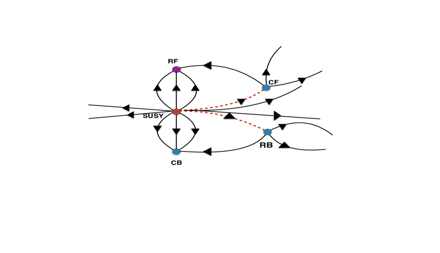
Figure 2: In this figure we present a qualitative sketch of the structure of large $\displaystyle N$ critical flows from theory S, constructed in Jain:2013gza , when the most relevant deformation is tuned to zero. We have added to their discussion the extra flows denoted by dashed red lines, which are further fine-tuned, from the supersymmetric theory to the quasi-bosonic theories.

As we have emphasized above, the flows described in this subsubsection and in Figure 2 are large $\displaystyle N$ flows, governed by the leading order beta functions that are of order unity in the large $\displaystyle N$ limit. The fact that we had to perform a two-parameter tuning to end up on the manifold of quasi-bosonic theories is a consequence of the fact that there are exactly two relevant directions away from the manifold of quasi-bosonic theories in the strict large $\displaystyle N$ limit .

At finite large $\displaystyle N$, the fast flows from theory S to the space of quasi-bosonic theories described in this subsection, generically do not end at true fixed points. Instead they terminate at some generic value of $\displaystyle x_{6}$ on the space of quasi-bosonic theories. After the fast flow is completed, the flow of $\displaystyle x_{6}$ continues at a much slower pace. The slow part of the flow is governed by the $\displaystyle\beta$ functions described in the previous subsubsection, and takes place over RG flow time scales of order $\displaystyle N$.

It turns out that the fast part of the RG flows hits the quasi-bosonic manifold between the second and third fixed point when $\displaystyle|\lambda_{B}|$ is smaller than some critical value of order unity, which lies between $\displaystyle 0$ and $\displaystyle 1$. The subsequent slow flow then ends up in the second (attractive) quasi-bosonic fixed point. For $\displaystyle|\lambda_{B}|$ less than this critical value, the flows constructed in this paper may thus be thought of as a ‘derivation’ of the duality between the second RB fixed point and the second CF fixed point, for finite large values of $\displaystyle N$, assuming the well-established duality of the supersymmetric theories S.

For $\displaystyle|\lambda_{B}|$ greater than the critical value described in the last paragraph, the fast flows constructed in this paper hit the manifold of quasi-bosonic theories at a value of $\displaystyle x_{6}$ larger than the third fixed point. The subsequent slow flow drives $\displaystyle x_{6}$ to infinity. See Figure 3 for a sketch of these two different classes of flows.

In the discussion above we have assumed the correctness of our conjecture that the beta function on the line of quasi-bosonic theories has three zeroes for every value of $\displaystyle\lambda$. It is possible that this conjecture is incorrect and that there is a range of values of $\displaystyle\lambda$ for which the beta function has only a single zero. In this case the single fixed point is always repulsive. RG flows from the SUSY theory that are tuned to land on the line of quasi-bosonic theories will always flow away from this fixed point – either to $\displaystyle x_{6}=\infty$ or to $\displaystyle x_{6}=-\infty$. We cannot generically tune a flow from the SUSY theory to hit such a fixed point, as it has $\displaystyle 3$ relevant deformations while flows originating at the SUSY theory have just two dimensionless parameters.

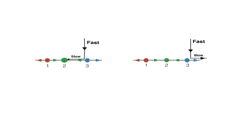
Figure 3: In this figure we depict two different classes of flows. The horizontal axis is $\displaystyle x_{6}$, and the vertical axis depicts the other parameters in the SUSY flow. The figure on the left, relevant for small $\displaystyle|\lambda_{B}|$, shows a fast flow arriving between the second and third fixed points, and a subsequent slow flow ending up in the second (attractive) quasi-bosonic fixed point. The figure on the right, relevant for large $\displaystyle|\lambda_{B}|$, shows a fast flow arriving at a value of $\displaystyle x_{6}$ larger than the third fixed point, and a subsequent slow flow driving $\displaystyle x_{6}$ to infinity.

We believe that the results of this subsection together with those of the previous subsection strongly suggest that the regular boson and critical fermion theories both exist, and are dual to each other, at all values of $\displaystyle\lambda$ and $\displaystyle x_{6}$ for infinite $\displaystyle N$, and also at least for large but finite $\displaystyle N$ and $\displaystyle\kappa$, when $\displaystyle x_{6}$ sits at its fixed points.

In section 4.5 we analyze an alternative way to flow to the quasi-fermionic and quasi-bosonic theories, by starting from a high-energy Yang-Mills-Chern-Simons theory. This flow makes sense for arbitrary values of $\displaystyle N$ and $\displaystyle\kappa$; note that for finite values of these numbers it is hard to tell if the formal definitions of these theories, (2)-(5), are well-defined or not. For finite values of $\displaystyle N$ and $\displaystyle\kappa$ it is hard to say when this flow ends at fixed points (after appropriate fine-tuning) and when it does not. In any case, this flow suggests that whenever we can end up at a quasi-fermionic theory, we can also end up at the corresponding quasi-bosonic theory, with one additional fine-tuning. This is subject to the same caveats as above, that there is a stable fixed point for $\displaystyle x_{6}$, and that the ‘fast flow’ governed by the Yang-Mills coupling brings us to the domain of attraction of this fixed point.

2 Critical scalars and regular fermions

As we have explained in the introduction, the simplest and best established non-supersymmetric Bose-Fermi duality in $\displaystyle 2+1$ dimensions is that between the CB and RF theories. In this section we review relevant aspects of these theories and their duality.

2.1 Critical scalars

2.1.1 Definitions

The critical scalar (CB) theory is a conformal field theory defined by the Lagrangian

$$\displaystyle S_{CB}(\phi,\sigma_{B}) \displaystyle=\int d^{3}x\biggl{[}i\varepsilon^{\mu\nu\rho}{\kappa_{B}\over 4\pi}\mathrm{Tr}(A_{\mu}\partial_{\nu}A_{\rho}-{2i\over 3}A_{\mu}A_{\nu}A_{\rho})+i\varepsilon^{\mu\nu\rho}{N_{B}\kappa^{\prime}_{B}\over 4\pi}B_{\mu}\partial_{\nu}B_{\rho}$$

$$\displaystyle~{}~{}~{}~{}~{}~{}~{}~{}~{}~{}~{}~{}~{}+D_{\mu}\bar{\phi}D^{\mu}\phi+\sigma_{B}\bar{\phi}\phi\biggl{]}.$$ (11)

Here $\displaystyle\kappa_{B}$ is the level of an $\displaystyle SU(N_{B})$ gauge field $\displaystyle A_{\mu}$ while $\displaystyle N_{B}\kappa^{\prime}_{B}$ is the level of a $\displaystyle U(1)$ gauge field $\displaystyle B_{\mu}$. The two join together into a $\displaystyle U(N_{B})=(SU(N_{B})\times U(1))/Z_{N_{B}}$ gauge field. Both $\displaystyle\kappa_{B}$ and $\displaystyle\kappa^{\prime}_{B}$ are non-zero integers. The fields $\displaystyle A_{\mu}$ are $\displaystyle N\times N$ traceless Hermitian matrices. The covariant derivative $\displaystyle D_{\mu}$ is given by

$$D_{\mu}\phi=\partial_{\mu}\phi+iA_{\mu}\phi+iB_{\mu}\phi.$$ (12)

The theory based on the action (11) is defined using the dimensional reduction scheme Siegel:1979wq . The same physical theory is obtained if one uses a Yang-Mills regulator and simultaneously replaces the levels $\displaystyle\kappa_{B}$ and $\displaystyle\kappa^{\prime}_{B}$ by the levels $\displaystyle k_{B}$ and $\displaystyle k^{\prime}_{B}$ given by (see Appendix D)

$$\kappa_{B}={\text{sgn}}(k_{B})\left(|k_{B}|+N_{B}\right),~{}~{}~{}\kappa^{\prime}_{B}=k^{\prime}_{B},$$ (13)

so that we must have $\displaystyle|\kappa_{B}|>N_{B}$. If we give a mass to the critical bosons (with a positive mass squared) and integrate them out, the resultant low energy theory is a pure $\displaystyle U(N_{B})$ Chern-Simons theory, whose levels $\displaystyle k_{B},k^{\prime}_{B}$ can be identified with the levels of the related $\displaystyle U(N_{B})$ WZW theories.

The critical boson theories defined so far are labeled by three integers: $\displaystyle N_{B}$, $\displaystyle\kappa_{B}$ and $\displaystyle\kappa^{\prime}_{B}$. In the rest of this paper we will be principally interested in the following three two-integer subfamilies of critical scalar theories:

• $\displaystyle SU(N_{B})$ critical scalars. These theories are defined by the Lagrangian (11) with $\displaystyle B_{\mu}$ set to zero. These theories are labeled either by the pair of integers $\displaystyle(N_{B},\kappa_{B})$ or $\displaystyle(N_{B},k_{B})$ according to taste.

• $\displaystyle U(N_{B})$ critical scalars of type 1. These are critical scalar theories with $\displaystyle\kappa^{\prime}_{B}=\kappa_{B}$, $\displaystyle k^{\prime}_{B}={\text{sgn}(k_{B})}(|k_{B}|+N_{B})$. These theories are also labeled by a pair of integers – again either $\displaystyle(N_{B},\kappa_{B})$ or $\displaystyle(N_{B},k_{B})$ according to taste.

• $\displaystyle U(N_{B})$ critical scalars of type 2. These are critical scalar theories with $\displaystyle k^{\prime}_{B}=k_{B}$, $\displaystyle\kappa_{B}={\text{sgn}(\kappa^{\prime}_{B})}(|\kappa^{\prime}_{B}|+N_{B})$. Once again these theories are labeled either by the integer pairs $\displaystyle(N_{B},\kappa_{B})$ or $\displaystyle(N_{B},k_{B})$ according to taste.

For each of the three families of theories above, we define the ’t Hooft coupling

$$\lambda_{B}=\frac{N_{B}}{\kappa_{B}}.$$ (14)

In the large $\displaystyle N_{B}$ limit, the theories above are most conveniently parameterized by the integer $\displaystyle N_{B}$ and the effectively continuous real parameter $\displaystyle\lambda_{B}$, obeying $\displaystyle|\lambda_{B}|<1$.

2.1.2 Review of useful results at large $\displaystyle N_{B}$

At leading order in the large $\displaystyle N_{B}$ limit the $\displaystyle SU(N_{B})$, type 1 and type 2 $\displaystyle U(N_{B})$ theories are all identical. Several results for these theories have been established for all values of $\displaystyle\lambda_{B}$ in this limit. We will now present a brief review of those results that will be of interest to us later in this paper.

Denote the lowest dimensional scalar operator in the critical boson theory by $\displaystyle{\tilde{J}}_{0}$. In the dimensional regularization scheme (in which operators of distinct bare dimension cannot mix) $\displaystyle{\tilde{J}}_{0}\propto\sigma_{B}$. We choose the normalization of $\displaystyle{\tilde{J}}_{0}$ as

$${\tilde{J}}_{0}=\sigma_{B}.$$ (15)

The scaling dimension $\displaystyle\Delta_{B}(\lambda_{B})$ of $\displaystyle{\tilde{J}}_{0}$ has the large $\displaystyle N_{B}$ expansion

$$\Delta_{B}(\lambda_{B})=2+\frac{\delta_{B}(\lambda_{B})}{\kappa_{B}}+{\cal O}(1/\kappa_{B}^{2}).$$ (16)

The function $\displaystyle\delta_{B}(\lambda_{B})$ is as yet unknown.

In the limit $\displaystyle\lambda_{B}\to 0$, which gives the critical $\displaystyle U(N_{B})$ vector model, the anomalous dimension is Vasiliev:1982dc

$$\frac{\delta_{B}(\lambda_{B})}{\kappa_{B}}=-\frac{16}{3\pi^{2}N_{B}}\implies\delta_{B}(\lambda_{B})=-\frac{16}{3\pi^{2}\lambda_{B}}.$$ (17)

In the large $\displaystyle N_{B}$ limit, the two-point function of $\displaystyle{\tilde{J}}_{0}$ is given by Aharony:2012nh

$$\begin{split}&\langle{\tilde{J}}_{0}(q){\tilde{J}}_{0}(-q^{\prime})\rangle=\frac{1}{\kappa_{B}}(2\pi)^{3}\delta^{3}(q-q^{\prime})G_{\sigma}(p),\\ &G_{\sigma}(q)=n_{B}q^{\left(2\Delta_{B}(\lambda_{B})-3\right)},\\ &n_{B}=-4\frac{\pi}{\tan(\frac{\pi\lambda_{B}}{2})}+{\cal O}(1/\kappa_{B}).\\ \end{split}$$ (18)

At leading order in large $\displaystyle N_{B}$ (18) reduces to

$$\langle{\tilde{J}}_{0}(q){\tilde{J}}_{0}(-q^{\prime})\rangle=(2\pi)^{3}\delta^{3}(q-q^{\prime})~{}~{}\frac{(-4\pi)|q|}{\kappa_{B}\tan(\frac{\pi\lambda_{B}}{2})}.$$ (19)

At small $\displaystyle\lambda_{B}$ this result further simplifies to

$$\langle{\tilde{J}}_{0}(q){\tilde{J}}_{0}(-q^{\prime})\rangle=(2\pi)^{3}\delta^{3}(q-q^{\prime})~{}~{}\frac{(-8)|q|}{N_{B}}\left(1+{\cal O}(\lambda_{B}^{2})\right).$$ (20)

Note that

$$\int\frac{d^{3}p}{(2\pi)^{3}}|p|e^{-\epsilon|p|}e^{ip\cdot r}=\frac{1}{2\pi^{2}r}\int_{0}^{\infty}dpp^{2}\sin(pr)e^{-\epsilon p}=-\frac{1}{\pi^{2}}\frac{r^{2}-3\epsilon^{2}}{(r^{2}+\epsilon^{2})^{3}}.$$ (21)

By taking the limit $\displaystyle\epsilon\to 0$ it follows that the Fourier transform of $\displaystyle-|p|$ is $\displaystyle\frac{1}{\pi^{2}r^{4}}$. It follows, in particular, that the two point functions (19) and (20) are all positive when reexpressed in position space, consistent with the expectations from unitarity.

The three point function of $\displaystyle{\tilde{J}}_{0}$ is given by

$$\begin{split}&\langle{\tilde{J}}_{0}(q_{1}){\tilde{J}}_{0}(q_{2}){\tilde{J}}_{0}(q_{3})\rangle=(2\pi)^{3}\delta^{3}(q_{1}+q_{2}+q_{3}){\tilde{G}}_{3}(q_{1},q_{2},q_{3}),\\ &{\tilde{G}}_{3}(q_{1},q_{2},q_{3})=\frac{32\pi^{2}}{\kappa_{B}^{2}}\left(c_{B}^{\delta}(\lambda_{B})+c_{B}(\lambda_{B})F(|q_{1}|,|q_{2}|,|q_{3}|,\frac{\delta_{B}}{\kappa_{B}})\right).\\ \end{split}$$ (23)

(23) simply asserts that the three point function of three $\displaystyle{\tilde{J}}_{0}(q_{1})$ operators is the sum of a contact term and a piece proportional to $\displaystyle F(q_{1},q_{2},q_{3},\frac{\delta_{B}}{\kappa_{B}})$, the Fourier transform of the usual power law position space expression for a three point function of three operators of dimension $\displaystyle 2+\frac{\delta_{B}}{\kappa_{B}}$. An explicit integral expression for $\displaystyle F(q_{1},q_{2},q_{3},\frac{\delta_{B}}{\kappa_{B}})$ was presented in Bzowski:2013sza ; using that expression we demonstrate in Appendix A that in the normalization we use

$$\frac{\delta_{B}}{|\kappa_{B}|}~{}F(q_{1},q_{2},q_{3},\frac{\delta_{B}}{\kappa_{B}})=1-3\frac{\delta_{B}}{\kappa_{B}}~{}\ln\left(\frac{\Lambda}{q_{1}+q_{2}+q_{3}}\right)+{\cal O}(\frac{1}{\kappa_{B}^{2}}),$$ (24)

note that $\displaystyle F(q_{1},q_{2},q_{3},\frac{\delta_{B}}{\kappa_{B}})$ reduces to a constant at leading order at $\displaystyle 1/N$ and deviates from the constant only at first sub-leading order. It follows that the contact piece in (23) and $\displaystyle F(q_{1},q_{2},q_{3},\frac{\delta_{B}}{\kappa_{B}})$ are indistinguishable at leading order at large $\displaystyle N$.

The three point functions of $\displaystyle{\tilde{J}}_{0}$ have been computed at leading order in the large $\displaystyle N$ limit. Comparing (23) to the explicit results of this computation we find Aharony:2012nh

$$\begin{split}&c_{B}^{\delta}(\lambda_{B})=r_{B}(\lambda_{B})\left(\frac{\cot^{2}(\frac{\pi\lambda_{B}}{2})}{\cos^{2}(\frac{\pi\lambda_{B}}{2})}-\frac{1}{4}\right)+{\cal O}(1/\kappa_{B}),\\ &c_{B}(\lambda_{B})=(1-r_{B}(\lambda_{B}))\frac{\delta_{B}}{\kappa_{B}}\left(\frac{\cot^{2}(\frac{\pi\lambda_{B}}{2})}{\cos^{2}(\frac{\pi\lambda_{B}}{2})}-\frac{1}{4}\right)+{\cal O}(1/|\kappa_{B}|^{2}),\\ \end{split}$$ (25)

where $\displaystyle r_{B}(\lambda_{B})$ is a parameter which has not yet been determined, because the three point function has been explicitly evaluated only at leading order at large $\displaystyle N$ where $\displaystyle F(q_{1},q_{2},q_{3},\frac{\delta_{B}}{\kappa_{B}})$ and the contact term in (23) can not be distinguished as we have explained above. Expanding (23) to first order in $\displaystyle{1\over\kappa_{B}}$ using (LABEL:thptdet), we find

$$\begin{split}{\tilde{G}}_{3}(q_{1},q_{2},q_{3})=&\frac{32\pi^{2}}{\kappa_{B}^{2}}\left(\frac{\cot^{2}(\frac{\pi\lambda_{B}}{2})}{\cos^{2}(\frac{\pi\lambda_{B}}{2})}-\frac{1}{4}\right)\cdot\\ &\cdot\left(\left(1+{\cal O}(\frac{1}{\kappa_{B}})\right)+3r_{B}(\lambda_{B})\frac{\delta_{B}}{\kappa_{B}}\ln\left(\frac{\Lambda}{|q_{1}|+|q_{2}|+|q_{3}|}\right)+{\cal O}(\frac{1}{\kappa_{B}^{2}})\right).\end{split}$$ (26)

Note that the non-analytic term in momenta in (26) starts out at order $\displaystyle{\cal O}(\frac{1}{\kappa_{B}})$. At leading order in the $\displaystyle\frac{1}{N_{B}}$ expansion

$$\begin{split}&\langle{\tilde{J}}_{0}(q_{1}){\tilde{J}}_{0}(q_{2}){\tilde{J}}_{0}(q_{3})\rangle=(2\pi)^{3}\delta^{3}(q_{1}+q_{2}+q_{3})~{}~{}\frac{32\pi^{2}}{\kappa_{B}^{2}}\left(\frac{\cot^{2}(\frac{\pi\lambda_{B}}{2})}{\cos^{2}(\frac{\pi\lambda_{B}}{2})}-\frac{1}{4}\right),\end{split}$$ (27)

and so the three point function is a pure contact term in accordance with general expectations Maldacena:2012sf .

Notice that the parameter $\displaystyle r_{B}(\lambda_{B})$ that appears in (LABEL:thptdet) disappears in the leading order result (27). This is the reason that $\displaystyle r_{B}(\lambda_{B})$ cannot be determined by a comparison with explicit leading large $\displaystyle N_{B}$ results, and so is unknown. As the term proportional to $\displaystyle r_{B}(\lambda_{B})$ in (26) multiplies a factor of $\displaystyle\ln(\Lambda)$, this term will contribute to the $\displaystyle\beta$ function computed later in this paper and so will be of importance to us. In Appendix B we present a formal expression for $\displaystyle r_{B}$ at $\displaystyle\lambda_{B}=0$.

At small $\displaystyle\lambda_{B}$ (27) simplifies further to

$$\begin{split}&\langle{\tilde{J}}_{0}(q_{1}){\tilde{J}}_{0}(q_{2}){\tilde{J}}_{0}(q_{3})\rangle=(2\pi)^{3}\delta^{3}(q_{1}+q_{2}+q_{3})~{}~{}\frac{128}{N_{B}^{2}}\left(1+{\cal O}(\lambda_{B}^{2})\right).\end{split}$$ (28)

The four point function of four scalar operators has also been recently computed at leading order in the large $\displaystyle N_{B}$ limit Turiaci:2018nua (see Aharony:2018npf ; Yacoby:2018yvy for further developments). The four point function takes the form

$$\langle{\tilde{J}}_{0}(q_{1}){\tilde{J}}_{0}(q_{2}){\tilde{J}}_{0}(q_{3}){\tilde{J}}_{0}(q_{4})\rangle=(2\pi)^{3}\delta^{3}(q_{1}+q_{2}+q_{3}+q_{4}){\tilde{G}}_{4}^{0}(q_{1},q_{2},q_{3},q_{4}),$$ (29)

where $\displaystyle{\tilde{G}}_{4}^{0}$ has mass dimension $\displaystyle(-1)$ (it is a homogeneous function of its arguments of homogeneity $\displaystyle(-1)$). It was demonstrated in Turiaci:2018nua that the momentum dependence of the four point function is the same as the momentum dependence of the operator $\displaystyle{\bar{\psi}}\psi$ in a theory of free fermions. The prefactor of this momentum dependence was also determined in Turiaci:2018nua . In this paper we will be principally interested in the four point function in a particular kinematical limit, namely the limit $\displaystyle\delta\to 0$ of $\displaystyle{\tilde{G}}_{4}^{0}(p,-p-\delta,k+\delta,-k)$. The $\displaystyle\delta\to 0$ limit of this correlator is smooth so the four point function in the kinematical limit of interest to us is simply $\displaystyle{\tilde{G}}_{4}^{0}(p,-p,k,-k)$. It turns out that

$$\begin{split}&{\tilde{G}}_{4}^{0}(p,-p,k,-k)=\\ &-2^{7}\left(\frac{2\pi}{\kappa_{B}}\right)^{3}\frac{1}{(\tan(\frac{\pi\lambda_{B}}{2}))^{2}\sin(\pi\lambda_{B})}\left(\frac{1}{2|k+p|}+\frac{1}{2|k-p|}-\frac{1}{2}\frac{|k|}{|p|^{2}}-\frac{1}{2}\frac{(p\cdot k)^{2}}{|p|^{4}|k|}+{\cal O}(k/p^{2})\right).\end{split}$$ (30)

In particular at $\displaystyle\lambda_{B}=0$ (see the explicit computation in Appendix B for a check)

$${\tilde{G}}_{4}^{0}(p,-p,k,-k)=-\frac{8^{4}}{N_{B}^{3}}\left(\frac{1}{2|k+p|}+\frac{1}{2|k-p|}-\frac{1}{2}\frac{|k|}{|p|^{2}}-\frac{1}{2}\frac{(p\cdot k)^{2}}{|p|^{4}|k|}+{\cal O}(k/p^{2})\right).$$ (31)

In a Taylor series expansion in $\displaystyle\frac{|k|}{|p|}$ we have

$${\tilde{G}}^{0}_{4}=\frac{1}{|p|\kappa_{B}^{3}}\left({\tilde{g}}_{(4,1)}+{\tilde{g}}_{(4,2)}\frac{|k|}{|p|}+{\tilde{g}}_{(4,3)}\frac{(p\cdot k)^{2}}{|p|^{3}|k|}+{\cal O}(k^{2}/p^{2})\right),$$ (32)

where

$${\tilde{g}}_{(4,1)}=-2{\tilde{g}}_{4},\qquad{\tilde{g}}_{(4,2)}={\tilde{g}}_{4},\qquad{\tilde{g}}_{(4,3)}={\tilde{g}}_{4},$$ (33)

with

$${\tilde{g}}_{4}=\frac{2^{9}\pi^{3}}{(\tan(\frac{\pi\lambda_{B}}{2}))^{2}\sin(\pi\lambda_{B})}.$$ (34)

Specifically in the limit $\displaystyle\lambda_{B}\to 0$

$${\tilde{g}}_{4}=\frac{1}{2}\frac{8^{4}}{\lambda_{B}^{3}}$$ (35)

so that

$${\tilde{g}}_{(4,1)}=-\frac{8^{4}}{\lambda_{B}^{3}},\qquad{\tilde{g}}_{(4,2)}=\frac{1}{2}\frac{8^{4}}{\lambda_{B}^{3}},\qquad{\tilde{g}}_{(4,3)}=\frac{1}{2}\frac{8^{4}}{\lambda_{B}^{3}}.~{}~{}~{}$$ (36)

For our purpose we also need the five point function

$$\langle{\tilde{J}}_{0}(q_{1}){\tilde{J}}_{0}(q_{2}){\tilde{J}}_{0}(q_{3}){\tilde{J}}_{0}(q_{4}){\tilde{J}}_{0}(q_{5})\rangle=(2\pi)^{3}\delta^{3}(q_{1}+q_{2}+q_{3}+q_{4}+q_{5}){\tilde{G}}_{5}^{0}(q_{1},q_{2},q_{3},q_{4},q_{5}),$$ (37)

where $\displaystyle{\tilde{G}}_{5}^{0}$ has mass dimension $\displaystyle(-2)$ (it is a homogeneous function of its arguments of homogeneity $\displaystyle(-2)$). For our purpose, we are just interested in the function $\displaystyle{\tilde{G}}_{5}^{0}(p,-p,0,0,0)$. It follows from dimensional analysis that this Green’s function admits a form

$${\tilde{G}}_{5}^{0}=\frac{1}{|p|^{2}\kappa_{B}^{4}}{\tilde{g}}_{(5,0)},$$ (38)

where $\displaystyle{\tilde{g}}_{(5,0)}$ is a number (which is a function of $\displaystyle\lambda_{B}$), whose value at $\displaystyle\lambda_{B}=0$ is discussed in appendix B.1.3.

2.1.3 $\displaystyle SO(N)$ theories

Throughout this paper we primarily discuss theories with unitary gauge groups (11). It is, however, useful to note that the results presented above also apply (with minor modifications) at leading order in large $\displaystyle N_{B}$ to the $\displaystyle SO(N_{B})$ gauged theory with action

$$S_{CB}(\phi,\sigma)=\int d^{3}x\biggl{[}i\varepsilon^{\mu\nu\rho}{\kappa_{B}\over 8\pi}\mathrm{Tr}(A_{\mu}\partial_{\nu}A_{\rho}-{2i\over 3}A_{\mu}A_{\nu}A_{\rho})+\frac{D_{\mu}\phi D^{\mu}\phi}{2}+\sigma_{B}\phi\phi\biggl{]},$$ (39)

where $\displaystyle A_{\mu}$ are now imaginary antisymmetric matrices – i.e. generators of $\displaystyle SO(N_{B})$. The ’t Hooft coupling is once again defined by $\displaystyle\lambda=\frac{N_{B}}{\kappa_{B}}$. The leading large $\displaystyle N_{B}$ $\displaystyle n$-point Green’s functions of the theory (39) at any particular value of the ’t Hooft coupling are obtained from the leading large $\displaystyle N_{B}$ Green’s functions of the theory (11) at the same value of the ’t Hooft coupling using the translation formulae

$${\tilde{G}}_{n}^{SO(N)}=\frac{1}{2}{\tilde{G}}_{n}^{SU(N)}.$$ (40)

2.2 The regular fermion theory

The regular fermion (RF) theory is defined by the Lagrangian

$$S_{CF}=\int d^{3}x\bigg{[}i\varepsilon^{\mu\nu\rho}{\kappa_{F}\over 4\pi}\mathrm{Tr}(A_{\mu}\partial_{\nu}A_{\rho}-{2i\over 3}A_{\mu}A_{\nu}A_{\rho})+i\varepsilon^{\mu\nu\rho}{\kappa^{\prime}_{F}\over 4\pi}B_{\mu}\partial_{\nu}B_{\rho}+\bar{\psi}\gamma_{\mu}D^{\mu}\psi\bigg{]}.$$ (41)

Our conventions for levels are the same as in the previous subsection. In particular the path integral with the action (41) is defined with the dimensional regulation scheme. We get the same physics with a Yang-Mills regulator if we modify the action above replacing $\displaystyle\kappa_{F}$ with $\displaystyle k_{F}$ and $\displaystyle\kappa^{\prime}_{F}$ with $\displaystyle k^{\prime}_{F}$ where

$$\kappa_{F}={\text{sgn}}(k_{F})\left(|k_{F}|+N_{F}\right),~{}~{}~{}\kappa^{\prime}_{F}=k^{\prime}_{F}.$$ (42)

One difference with the theories of the previous subsection is that $\displaystyle\kappa_{F}$ and $\displaystyle k_{F}$ are half integers (numbers of the form $\displaystyle\frac{2n+1}{2}$ with integer $\displaystyle n$) in our notation rather than integers. This can be understood in the following terms. If we add a mass term with mass parameter $\displaystyle m_{F}$ to the Lagrangian (41) and integrate the fermion out then the resulting gauge theory, at long distances, is a pure Chern-Simons theory with Chern-Simons level (equal to the level of the dual WZW theory) equal to $\displaystyle(k_{F}+\frac{\text{sgn}(m_{F})}{2})$. This level is an integer, as it has to be, if and only if $\displaystyle k_{F}$ is a half integer, and this defines what we mean by half-integer levels.

It is convenient to define

$${\tilde{\kappa}}_{F}=\kappa_{F}+\frac{\text{sgn}(\kappa_{F})}{2}.$$ (43)

The quantity $\displaystyle{\tilde{\kappa}}_{F}$ agrees with the effective value of $\displaystyle\kappa$ for the low energy pure Chern-Simons theory obtained after integrating out the fermion, when it is given a mass of the same sign as $\displaystyle\kappa_{F}$. We define the fermionic ’t Hooft coupling by the equation

$$\lambda_{F}=\frac{N_{F}}{{\tilde{\kappa}}_{F}}.$$ (44)

It follows that $\displaystyle\lambda_{F}$ is simply the standard definition of the ’t Hooft coupling for the effective low energy Chern-Simons theory obtained after integrating out the fermions with a mass of the same sign as $\displaystyle{\tilde{\kappa}_{F}}$.

As in the previous subsection we have $\displaystyle SU(N_{F})$, type 1 $\displaystyle U(N_{F})$ and type 2 $\displaystyle U(N_{F})$ regular fermion theories. The definition of these theories is the obvious fermionic analogue of the definitions of the previous subsection.

2.2.1 Review of results at large $\displaystyle N_{F}$

As in the previous subsection, the lowest dimension scalar field $\displaystyle J_{0}$ in this theory will play an important role in what follows. In the dimensional reduction scheme (and with an appropriate choice of normalization that we adopt)

$$J^{F}_{0}=\frac{4\pi{\bar{\psi}}\psi}{{\tilde{\kappa}_{F}}}.$$ (45)

The dimension of this operator is given by

$$\Delta_{F}(\lambda_{F})=2-\frac{\delta_{F}(\lambda_{F})}{{\tilde{\kappa}_{F}}}+{\cal O}(1/{\tilde{\kappa}_{F}}^{2})$$ (46)

where $\displaystyle\delta_{F}(\lambda_{F})=-\frac{4}{3}\lambda_{F}+O(\lambda_{F}^{2})$ (see equation (5.32) of Giombi:2016zwa ).

In the large $\displaystyle N_{F}$ limit the two point function of $\displaystyle J^{F}_{0}$ is given by Aharony:2012nh

$$\begin{split}&\langle J^{F}_{0}(q)J^{F}_{0}(-q^{\prime})\rangle=\frac{1}{{\tilde{\kappa}_{F}}}(2\pi)^{3}\delta^{3}(q-q^{\prime})n_{F}q^{\left(2\Delta_{F}(\lambda_{F})-3\right)},\\ &n_{F}=-4\pi\tan\left(\frac{\pi\lambda_{F}}{2}\right)+{\cal O}(1/{\tilde{\kappa}_{F}}).\\ \end{split}$$ (47)

At leading order in large $\displaystyle\kappa_{F}$, the small $\displaystyle\lambda_{F}$ expansion of (47) gives

$$\langle J^{F}_{0}(q)J^{F}_{0}(-q^{\prime})\rangle=-(2\pi)^{3}\delta^{3}(q-q^{\prime})2\pi^{2}|q|N_{F}\frac{1}{{\tilde{\kappa}}_{F}^{2}}+{\cal O}(\lambda_{F}^{2}).$$ (48)

Three point functions of $\displaystyle J_{0}^{F}$ take the form Aharony:2012nh

$$\begin{split}&\langle{J}^{F}_{0}(q_{1}){J}^{F}_{0}(q_{2}){J}^{F}_{0}(q_{3})\rangle=\frac{(2\pi)^{3}}{{\tilde{\kappa}_{F}}^{2}}\delta^{3}(q_{1}+q_{2}+q_{3})\left(c_{F}^{\delta}(\lambda_{F})+c_{F}(\lambda_{F})F(|q_{1}|,|q_{2}|,|q_{3}|,\frac{\delta_{F}}{{\tilde{\kappa}_{F}}})\right),\\ &c_{F}^{\delta}(\lambda_{F})=r_{F}(\lambda_{F})32\pi^{2}\tan^{2}\left(\frac{\pi\lambda_{F}}{2}\right)+{\cal O}(1/{\tilde{\kappa}_{F}}),\\ &c_{F}(\lambda_{F})=\frac{\delta_{F}}{{\tilde{\kappa}_{F}}}\left(1-r_{F}(\lambda_{F})\right)32\pi^{2}\tan^{2}\left(\frac{\pi\lambda_{F}}{2}\right)+{\cal O}(1/|{\tilde{\kappa}_{F}}|^{2}).\end{split}$$ (49)

The small $\displaystyle\lambda_{F}$ expansion of (49) gives

$$\langle{J}^{F}_{0}(q_{1}){J}^{F}_{0}(q_{2}){J}^{F}_{0}(q_{3})\rangle=(2\pi)^{3}\delta^{3}(q_{1}+q_{2}+q_{3})8\pi^{2}N_{F}\frac{\pi^{2}}{{\tilde{\kappa}_{F}}^{3}}\lambda_{F}+{\cal O}(\lambda_{F}^{4}).$$ (50)

Note, in particular, that the three point function vanishes in the limit $\displaystyle\lambda_{F}\to 0$. This is a consequence of the fact that the operator $\displaystyle{\bar{\psi}}\psi=\frac{\kappa_{F}}{4\pi}J_{0}^{F}$ is odd under parity transformations in the limit $\displaystyle\lambda_{F}\to 0$. As the left-hand side of (50) is odd under parity, while the $\displaystyle\delta$ function on the right-hand side is even, parity invariance forces the coefficient to vanish.

As in the previous subsection we restrict our discussion to the four point function leading order in the large $\displaystyle N_{F}$ limit. At this order the four point function is completely known. The momentum dependence of this function is precisely that of the free fermi theory Turiaci:2018nua (see Bedhotiya:2015uga for related earlier work). As in the previous subsection we define

$$\langle{J}_{0}(p_{1}){J}_{0}(p_{2}){J}_{0}(p_{3}){J}_{0}(p_{4})\rangle=(2\pi)^{3}\delta^{3}(p_{1}+p_{2}+p_{3}+p_{4}){G}_{4}^{0}(p_{1},p_{2},p_{3},p_{4})$$ (51)

where $\displaystyle G_{4}^{0}$ has mass dimension $\displaystyle(-1)$. Again we are interested in $\displaystyle G_{4}^{0}(p,-p,k,-k)$ in the limit $\displaystyle|k|\ll|p|$. Expanding the Greens function in a Taylor series expansion in $\displaystyle\frac{|k|}{|p|}$ we have

$${G}^{0}_{4}=-\frac{1}{|p|{\kappa}_{F}^{3}}\left({g}_{(4,1)}+{g}_{(4,2)}\frac{|k|}{|p|}+{g}_{(4,3)}\frac{(p\cdot k)^{2}}{|p|^{3}|k|}+{\cal O}(k^{2}/p^{2})\right),$$ (52)

$${g}_{(4,1)}=-2{g}_{4},\qquad{g}_{(4,2)}={g}_{4},\qquad{g}_{(4,3)}={g}_{4},$$ (53)

with

$${g}_{4}=-\frac{2^{9}\pi^{3}}{(\cot(\frac{\pi\lambda_{F}}{2}))^{2}\sin(\pi\lambda_{F})}$$ (54)

In particular in the limit $\displaystyle\lambda_{F}=0$ (see Appendix C for an explicit check) we find

$$G_{4}^{0}(p,-p,k,-k)=-N_{F}\left(\frac{4\pi}{\kappa_{F}}\right)^{4}\left(\frac{1}{|p|}-\frac{1}{2}\frac{|k|}{|p|^{2}}-\frac{1}{2}\frac{(p\cdot k)^{2}}{|p|^{4}|k|}+{\cal O}(k^{2}/p^{2})\right),$$ (55)

from which it follows that at leading order in small $\displaystyle\lambda_{F}$

$$g_{4}=-\frac{1}{2}(4\pi)^{4}\lambda_{F}$$

so that

$$g_{(4,1)}=(4\pi)^{4}\lambda_{F},\qquad g_{(4,2)}=-\frac{1}{2}(4\pi)^{4}\lambda_{F},\qquad g_{(4,3)}=-\frac{1}{2}(4\pi)^{4}\lambda_{F}.$$ (56)

For our purpose we also need the five point function

$$\langle J^{F}_{0}(q_{1})J^{F}_{0}(q_{2})J^{F}_{0}(q_{3})J^{F}_{0}(q_{4})J^{F}_{0}(q_{5})\rangle=(2\pi)^{3}\delta^{3}(q_{1}+q_{2}+q_{3}+q_{4}+q_{5})G_{5}^{0}(q_{1},q_{2},q_{3},q_{4},q_{5})$$ (57)

where $\displaystyle G_{5}^{0}$ has mass dimension $\displaystyle(-2)$ (it is a homogeneous function of its arguments of homogeneity $\displaystyle(-2)$). In the specific case $\displaystyle G_{5}^{0}(p,-p,0,0,0)$ this Green’s function takes the form

$$G_{5}^{0}=\frac{1}{|p|^{2}\kappa_{F}^{4}}{g}_{(5,0)}$$ (58)

where $\displaystyle g_{(5,0)}$ is a number (which is a function of $\displaystyle\lambda_{F}$). In the limit $\displaystyle\lambda_{F}\to 0$ parity forces

$${g}_{(5,0)}=0.$$ (59)

2.3 Duality

The critical boson and regular fermion theories have been conjectured to be related to each other via three different dualities (written here for a single matter field):

• $\displaystyle SU(N)$ regular fermion theories at (Yang-Mills regulated) level $\displaystyle k$ are dual to type 2 $\displaystyle U(|k|+\frac{1}{2})$ critical boson theories at level $\displaystyle-{\text{sgn}(k)}N$.

• Type 2 $\displaystyle U(N)$ regular fermion theories at (Yang-Mills regulated) level $\displaystyle k$ are dual to $\displaystyle SU(|k|+\frac{1}{2})$ critical boson theories at level $\displaystyle-{\text{sgn}(k)}N$.

• Type 1 $\displaystyle U(N)$ regular fermion theories at (Yang-Mills regulated) level $\displaystyle k$ are dual to $\displaystyle U(|k|+\frac{1}{2})$ Type 1 critical boson theories at (Yang-Mills regulated) level $\displaystyle-{\text{sgn}(k)}N$.

At leading order in the ’t Hooft large $\displaystyle N$ limit, the duality maps described above become identical, and can all be restated in the following form:

$$\lambda_{F}=-\text{sgn}(\lambda_{B})(1-|\lambda_{B}|),\qquad\qquad\frac{N_{F}}{|\lambda_{F}|}=\frac{N_{B}}{|\lambda_{B}|},\qquad\qquad{\tilde{\kappa}}_{F}=-\kappa_{B}.$$ (60)

Under this duality map the correlators of $\displaystyle J^{F}_{0}$ are identical at leading order to the correlators of $\displaystyle{\tilde{J}}_{0}$, up to a contact term in the three point function. Specifically

$$\begin{split}&\langle{J}^{F}_{0}(q_{1}){J}^{F}_{0}(q_{2})\rangle=\langle{\tilde{J}}_{0}(q_{1}){\tilde{J}}_{0}(q_{2})\rangle,\\ &\langle{J}^{F}_{0}(q_{1}){J}^{F}_{0}(q_{2}){J}^{F}_{0}(q_{3})\rangle=\langle{\tilde{J}}_{0}(q_{1}){\tilde{J}}_{0}(q_{2}){\tilde{J}}_{0}(q_{3})\rangle-\frac{6(2\pi)^{2}}{\kappa_{B}^{2}}~{}(2\pi)^{3}\delta(q_{1}+q_{2}+q_{3}),\\ &\langle{J}^{F}_{0}(q_{1}){J}^{F}_{0}(q_{2}){J}^{F}_{0}(q_{3}){J}^{F}_{0}(q_{4})\rangle=\langle{\tilde{J}}_{0}(q_{1}){\tilde{J}}_{0}(q_{2}){\tilde{J}}_{0}(q_{3}){\tilde{J}}_{0}(q_{4})\rangle.\\ \end{split}$$ (61)

The shift in contact terms between three point functions listed in (LABEL:jcorrs) follows by comparing (LABEL:thptdet) and (49) and using (65) below.

The conjectured duality between these two theories suggests that the match of correlation functions reported above persists – up to contact terms and the shift of $\displaystyle k$ above – to all orders in the $\displaystyle 1/N$ expansion. The contact term appearing in (LABEL:jcorrs) was computed only in the large $\displaystyle N$ limit. More generally the fermionic and bosonic three point functions are conjectured to be related via

$$\langle{J}^{F}_{0}(q_{1}){J}^{F}_{0}(q_{2}){J}^{F}_{0}(q_{3})\rangle-\langle{\tilde{J}}_{0}(q_{1}){\tilde{J}}_{0}(q_{2}){\tilde{J}}_{0}(q_{3})\rangle=-\frac{3!(2\pi)^{2}}{\kappa_{B}^{2}}(1+{\cal O}(\frac{1}{\kappa_{B}}))~{}(2\pi)^{3}\delta(q_{1}+q_{2}+q_{3}).$$ (62)

At leading order at large $\displaystyle N$ bosonic and fermionic answer map to each other under duality. In particular, under the duality map it is easily verified that

$${\tilde{g}}_{(4,1)}={g}_{(4,1)},\qquad{\tilde{g}}_{(4,2)}={g}_{(4,2)},\qquad{\tilde{g}}_{(4,3)}={g}_{(4,3)}.$$ (63)

Although five point functions have not explicitly been computed on either the bosonic or fermionic sides, the conjectured duality between the two theories leads us to expect that

$${\tilde{g}}_{(5,0)}={g}_{(5,0)}.$$ (64)

The fact that three point functions must agree at separated points implies that

$$(1-r_{B}(\lambda_{B}))\left(\frac{\cot^{2}(\frac{\pi\lambda_{B}}{2})}{\cos^{2}(\frac{\pi\lambda_{B}}{2})}-\frac{1}{4}\right)=\left(1-r_{F}(\lambda_{F})\right)\tan^{2}\left(\frac{\pi\lambda_{F}}{2}\right).$$ (65)

(63) is to be understood as follows. All terms of the left-hand side are evaluated at an arbitrary value of $\displaystyle\lambda_{B}$. All terms on the right-hand side are evaluated at an arbitrary value of $\displaystyle\lambda_{F}$. The equality in (63) holds provided $\displaystyle\lambda_{B}$ and $\displaystyle\lambda_{F}$ are related by (60).

The assumption of duality also implies that the anomalous dimensions of $\displaystyle{\tilde{J}}_{0}$ and $\displaystyle J_{0}^{F}$ are related; specializing to first subleading order in the $\displaystyle 1/N$ expansion this implies that

$$\delta_{B}(\lambda_{B})=\delta_{F}(\lambda_{F}),$$ (66)

provided $\displaystyle\lambda_{B}$ and $\displaystyle\lambda_{F}$ are related by (60).

More generally, using (62), the duality between the CB and RF theories implies the following relationship between the sourced partition functions of the bosonic and fermionic theories

$$\int D\phi D\sigma e^{-S_{cb}(\phi,\sigma)+\int{\tilde{J}}_{0}(x)\zeta(x)-\frac{(2\pi)^{2}}{\kappa_{B}^{2}}(1+{\cal O}(\frac{1}{\kappa_{B}}))\int\zeta^{3}(x)}=\int D\psi e^{-S_{rf}(\psi)+\int J_{0}^{F}(x)\zeta(x)}.$$ (67)

In this subsection we have, so far, discussed the $\displaystyle U(N)$ theory. There is a similar duality for $\displaystyle SO(N)$ theories (see Aharony:2016jvv for details), and using (40) it follows that for $\displaystyle SO(N)$

$$\int D\phi D\sigma e^{-S_{cb}(\phi,\sigma)+\int{\tilde{J}}_{0}(x)\zeta(x)-\frac{(2\pi)^{2}}{2\kappa_{B}^{2}}(1+{\cal O}(\frac{1}{\kappa_{B}}))\int\zeta^{3}(x)}=\int D\psi e^{-S_{rf}(\psi)+\int J_{0}^{F}(x)\zeta(x)}.$$ (68)

2.4 Duality from thermal partition functions

The spectrum of operators of the CB $\displaystyle\sim$ RF theories includes a single relevant scalar operator $\displaystyle{\tilde{J}}_{0}\sim J_{0}^{F}$ (here $\displaystyle\sim$ denotes equality under duality). It follows that the RG flow that originates at the CB $\displaystyle\sim$ RF theory is unique, and corresponds to deforming the conformal theory by $\displaystyle m{\tilde{J}}_{0}$.

It is possible to study these RG flows as a function of scale by computing the free energy of the mass-deformed theories described above as a function of the temperature. This calculation may be performed in the large $\displaystyle N$ limit, as we now review (see Aharony:2012ns ; Jain:2013py ; Takimi:2013zca for details).

Consider the mass-deformed critical boson theory defined by the action

$$S=S_{CB}(\phi,\sigma)+\frac{N_{B}}{4\pi}\int m_{B}^{cri}\sigma=S_{CB}+\frac{N_{B}}{4\pi}\int m_{B}^{cri}{\tilde{J}}_{0}.$$ (69)

Similarly consider the mass-deformed regular fermion theory

$$S=S_{RF}(\psi)+\int m_{F}^{reg}\bar{\psi}\psi=S_{RF}(\psi)+\frac{{\tilde{\kappa}}_{F}}{4\pi}\int m_{F}^{reg}{J}^{F}_{0}.$$ (70)

The conjectured duality between the critical boson and regular fermion theories leads us to expect that equations (69) and (70) define the same theory provided that

$$\frac{N_{B}}{4\pi}m_{B}^{cri}=\frac{{\tilde{\kappa}}_{F}}{4\pi}m_{F}^{reg}\qquad\implies\qquad m_{F}^{reg}=-\lambda_{B}m_{B}^{cri}.$$ (71)

We will now review evidence that this is indeed the case.

The finite temperature partition function of these theories on $\displaystyle S^{2}$ was computed, as a function of holonomies around the thermal circle, in Jain:2013py . As we are in the large $\displaystyle N$ limit, the result depends on eigenvalues only through an eigenvalue density function, $\displaystyle\rho_{B}(\alpha)$ (in the case of the bosonic theory) and $\displaystyle\rho_{F}(\alpha)$ (in the case of the fermionic theory). This computation proceeds as follows. One first sums Feynman diagrams to determine ‘offshell’ partition functions

$$Z_{B}=e^{-T^{2}V_{2}F_{B}[\rho_{B}(\alpha),c_{B}]},~{}~{}~{}Z_{F}=e^{-T^{2}V_{2}F_{F}[\rho_{F}(\alpha),c_{F}]}.$$ (72)

These partition functions are offshell because they depend on the additional variables $\displaystyle c_{B}$ and $\displaystyle c_{F}$, which have physical interpretations as the thermal pole masses of the bosonic and fermionic theories, respectively, in units of the temperature. The actual partition function is given by extremizing $\displaystyle F_{B}$ and $\displaystyle F_{F}$ with respect to $\displaystyle c_{B}$ and $\displaystyle c_{F}$, respectively, and plugging these extremized values into (72).

The explicit results for $\displaystyle F_{B}$ and $\displaystyle F_{F}$, obtained by summing the appropriate infinite class of Feynman diagrams, are (see, for example, equations (3.7) and (3.12) of Jain:2013gza and also the recent paper Choudhury:2018iwf for the bosonic computation in the Higgsed phase)

$$\begin{split}F_{B}[\rho_{B}(\alpha),c_{B}]&=\frac{N_{B}}{6\pi}{\Bigg{[}}-\frac{\left(\lambda_{B}-{\rm sgn}(\lambda_{B})-{\rm sgn}(X_{B})\right)}{\lambda_{B}}|c_{B}|^{3}+\frac{3}{2}{\hat{m}}_{B}^{cri}c_{B}^{2}\\ &+3\int_{-\pi}^{\pi}\rho_{B}(\alpha)d\alpha\int_{|c_{B}|}^{\infty}dyy\left(\ln\left(1-e^{-y-i\alpha}\right)+\ln\left(1-e^{-y+i\alpha}\right)\right){\Bigg{]}},\\ F_{F}[\rho_{B}(\alpha),c_{F}]&=\frac{N_{F}}{6\pi}{\Bigg{[}}|c_{F}|^{3}\frac{\left(\lambda_{F}-\text{sgn}(X_{F})\right)}{\lambda_{F}}+\frac{3}{2\lambda_{F}}{\hat{m}}_{F}^{reg}c_{F}^{2}\\ &-3\int_{-\pi}^{\pi}\rho_{F}(\alpha)d\alpha\int_{|c_{F}|}^{\infty}dyy\left(\ln\left(1+e^{-y-i\alpha}\right)+\ln\left(1+e^{-y+i\alpha}\right)\right){\Bigg{]}},\\ X_{F}&=2\lambda_{F}{\cal C}+{\hat{m}}_{F}^{reg},\\ X_{B}&=2\lambda_{B}{\cal S}-{\rm sgn}(\lambda_{B})|c_{B}|-m_{B}^{{\rm cri}}\lambda_{B},\end{split}$$ (73)

where $\displaystyle{\hat{m}}_{B}^{cri}$ and $\displaystyle{\hat{m}}_{F}^{reg}$ are the masses divided by the temperature.

As explained above, in order to evaluate the actual partition function of our theory we are instructed to extremize $\displaystyle F_{B}$ ($\displaystyle F_{F}$) with respect to $\displaystyle c_{B}$ and $\displaystyle c_{F}$. The condition that $\displaystyle F$ be extremized gives us an equation – called a gap equation – that can be used to determine $\displaystyle c_{B}$ and $\displaystyle c_{F}$, respectively. The gap equation for the bosonic theory takes the form

$$2{\cal S}-\frac{\left({\rm sgn}(\lambda_{B})+{\rm sgn}(X_{B})\right)}{\lambda_{B}}|{\hat{c}}_{B}|={\hat{m}}_{B}^{{\rm cri}}.$$ (76)

The gap equation for the fermionic theory is

$$|c_{F}|=\text{sgn}(X_{F})\left(2\lambda_{F}{\cal C}+{\hat{m}}_{F}^{{\rm reg}}\right),$$ (77)

where

$$\begin{split}{\cal C}=&\frac{1}{2}\int d\alpha\rho_{F}(\alpha)\left(\log(2\cosh(\frac{|c_{F}|+i\alpha}{2}))+\log(2\cosh(\frac{|c_{F}|-i\alpha}{2}))\right),\\ {\cal S}=&\frac{1}{2}\int d\alpha\rho_{B}(\alpha)\left(\log(2\sinh(\frac{|c_{B}|+i\alpha}{2}))+\log(2\sinh(\frac{|c_{B}|-i\alpha}{2}))\right).\end{split}$$ (78)

The bosonic and fermionic holonomy eigenvalue distribution functions are related to each other by the formula (see Jain:2013py )

$$|\lambda_{B}|\rho_{B}(\alpha)+|\lambda_{F}|\rho_{F}(\pi-\alpha)=\frac{1}{2\pi}.$$ (79)

When (79) holds it is easily verified that

$$\lambda_{B}{\cal S}=-\frac{\text{sgn}(\lambda_{F})}{2}|c_{F}|+\lambda_{F}{\cal C},\qquad\qquad\lambda_{F}{\cal C}=-\frac{\text{sgn}(\lambda_{B})}{2}|c_{B}|+\lambda_{B}{\cal S},$$ (80)

where $\displaystyle\lambda_{B}$ and $\displaystyle\lambda_{F}$ are related as in (60).

Using (80) and the first line of (60) it is easily verified that the bosonic and fermionic offshell free energies (73) – and so the gap equations (76) and (77) that follow from their extremization – turn into each other (up to the addition of the physically insignificant cosmological constant counter-terms mentioned above) when the couplings of the two theories are identified by (60) and the masses of the two theories are related by (71). This agreement gives powerful independent evidence for the duality between the CB and RF theories.

2.5 Phase Structure at zero temperature

The analysis of the previous section allows us immediately – and very simply – to determine the phase structure of the RF and CB theories at zero temperature. This analysis is facilitated by the fact that the zero temperature limit of the gap equations and offshell free energies reported in the previous subsection are particularly simple. In this limit $\displaystyle|c_{B}|$ and $\displaystyle|c_{F}|$ both tend to infinity and

$${\cal C}=\frac{|c_{F}|}{2},~{}~{}~{}~{}{\cal S}=\frac{|c_{B}|}{2},~{}~{}~{}X_{F}=\lambda_{F}|c_{F}|+{\hat{m}}_{F}^{reg}.$$ (82)

After dropping constant terms, the expressions (73) for the free energy reduce to

$$\begin{split}F_{B}[\rho_{B}(\alpha),c_{B}]&=\frac{N_{B}}{6\pi}\left(-\frac{\left(\lambda_{B}-{\rm sgn}(\lambda_{B})-{\rm sgn}(X_{B})\right)}{\lambda_{B}}|c_{B}|^{3}+\frac{3}{2}{\hat{m}}_{B}^{cri}c_{B}^{2}\right),\\ F_{F}[\rho_{B}(\alpha),c_{F}]&=\frac{N_{F}}{6\pi}\left(|c_{F}|^{3}\frac{\left(\lambda_{F}-\text{sgn}(X_{F})\right)}{\lambda_{F}}+\frac{3}{2\lambda_{F}}{\hat{m}}_{F}^{reg}c_{F}^{2}\right).\end{split}$$ (83)

The bosonic gap equation (which can be obtained either as the zero temperature limit of (76) or from the variation of the first of (83)) simplifies to

$$\frac{\left(\lambda_{B}-{\rm sgn}(\lambda_{B})-{\rm sgn}(X_{B})\right)}{\lambda_{B}}|c_{B}|={\hat{m}}_{B}^{cri}.$$ (84)

When $\displaystyle X_{B}\lambda_{B}<0$ (i.e. in the unHiggsed phase) this equation simplifies to

$$|c_{B}|={\hat{m}}_{B}^{cri};$$ (85)

in other words the unHiggsed gap equation has exactly one solution when $\displaystyle m_{B}^{\rm cri}$ is positive, but no solutions when $\displaystyle m_{B}^{\rm cri}$ is negative. Let us now turn to Higgsed solutions. In terms of the variable

$${\hat{\lambda}}_{B}=-{\rm sgn}(\lambda_{B})(2-|\lambda_{B}|)$$ (86)

the Higgsed zero temperature gap equation reduces to

$$\frac{{\hat{\lambda}}_{B}}{\lambda_{B}}|c_{B}|=m_{B}^{{\rm cri}}.$$ (87)

As $\displaystyle\frac{{\hat{\lambda}}_{B}}{\lambda_{B}}$ is always negative, it follows that there exists exactly one Higgsed vacuum whenever $\displaystyle m_{B}^{{\rm cri}}$ is negative, and no Higgsed vacua when $\displaystyle m_{B}^{{\rm cri}}$ is positive.

In summary the bosonic theory has a unique unHiggsed vacuum when $\displaystyle m_{B}^{{\rm cri}}$ is positive and a unique Higgsed vacuum whenever $\displaystyle m_{B}^{{\rm cri}}$ is negative. It follows that the CB theory undergoes a (second order) phase transition, from a unHiggsed to the Higgsed phase, as $\displaystyle m_{B}^{{\rm cri}}$ passes from positive to negative.

The fermionic gap equation (which can be obtained either as the zero temperature limit of (77) or from the variation of the second of (83)) simplifies to

$$|c_{F}|=\frac{|m_{F}|}{1-|\lambda_{F}|}$$ (88)

when

$${m_{F}^{\rm reg}}\geq 0,$$ (89)

and to

$$|c_{F}|=\frac{|{\hat{m}}_{F}^{reg}|}{1+|\lambda_{F}|}$$ (90)

when

$${\hat{m}}_{F}^{reg}\lambda_{F}<0.$$ (91)

Under the duality map, the condition (89) maps to the $\displaystyle m_{B}^{{\rm cri}}\geq 0$ condition and (88) maps to (85), while the converse condition (91) maps to the condition $\displaystyle m_{B}^{{\rm cri}}<0$ and (90) maps to (87). In other words the Fermionic theory in the parametric regime (89) maps to the critical boson theory in its unHiggsed phase, while the fermionic theory in the regime (91) maps to the CB theory in the Higgsed phase.

We end this section with a brief discussion of a confusing point. Focusing on the bosonic theory, we have explained above that the large $\displaystyle N$ free energies in our theories are obtained by extremizing an offshell free energy with respect to $\displaystyle|c_{B}|$. This fact may tempt the reader to view the offshell free energy as a Landau Ginzburg free energy for the ‘order parameter’ $\displaystyle|c_{B}|$ or $\displaystyle|c_{F}|$. In our view it is unclear that this is a correct viewpoint, or even what precisely this viewpoint might mean.

To see this, note that the zero temperature offshell free energy reported in (83) can be more explicitly rewritten as

$$\begin{split}&F_{B}[\rho_{B}(\alpha),c_{B}]\\ &=\frac{N_{B}}{6\pi}\left(-|c_{B}|^{3}+\frac{3}{2}{\hat{m}}_{B}^{cri}|c_{B}|^{2}\right)~{}~{}~{}{\rm when}~{}{\hat{m}}_{B}^{cri}>0,~{}~{}~{}{\rm~{}(unhiggsed)}\\ &=\frac{N_{B}}{6\pi}\left(|c_{B}|^{3}\frac{\left(2-|{\lambda}_{B}|\right)}{{\lambda}_{B}}+\frac{3}{2}|{\hat{m}}_{B}^{cri}||c_{B}|^{2}\right)~{}~{}~{}{\rm when}~{}{\hat{m}}_{B}^{cri}<0.~{}~{}~{}{\rm~{}(Higgsed)}\end{split}$$ (92)

It is clear from this equation that the zero mass limit of the off shell potential for $\displaystyle|c_{B}|$ is different depending on whether the mass approaches zero from above or below, while a genuine ‘Landau Ginzburg’ potential should be well-defined at every value of the mass including zero.

Conservatively one should regard the offshell free energy as no more than an intermediate device to be used for the computation of the onshell free energy. It would be interesting to find a genuine Landau Ginzburg potential for these theories and use it to analyze their stability etc. We leave this interesting task for future work.

3 Regular scalars and critical fermions and their RG flows

3.1 Definitions

The regular bosonic theory (RB) is defined by the action

$$S_{RB}(\phi,\sigma,\zeta)=S_{CB}(\phi,\sigma)-\int\sigma(x)\zeta(x)+\frac{(2\pi)^{2}}{\kappa_{B}^{2}}\left(x_{6}^{B}+1\right)\int\zeta^{3}(x).$$ (93)

Equivalently

$$S_{RB}(\phi,\sigma,\zeta)=S_{CB}(\phi,\sigma)-\int{\tilde{J}}_{0}(x)\zeta(x)+\frac{(2\pi)^{2}}{\kappa_{B}^{2}}\left(x_{6}^{B}+1\right)\int\zeta^{3}(x).$$ (94)

Here $\displaystyle S_{CB}(\phi,\sigma)$ is the action (11) for the critical bosonic theory, $\displaystyle\zeta$ is a new dynamical field and $\displaystyle x_{6}^{B}$ is a parameter.

If we insert (11) into (94) and integrate out $\displaystyle\sigma$ we find that the action in (94) reduces to the regular boson action

$$\begin{split}&S_{RB}(\phi)=\int d^{3}x\biggl{[}i\varepsilon^{\mu\nu\rho}{\kappa_{B}\over 4\pi}\mathrm{Tr}(A_{\mu}\partial_{\nu}A_{\rho}-{2i\over 3}A_{\mu}A_{\nu}A_{\rho})+i\varepsilon^{\mu\nu\rho}{N_{B}\kappa^{\prime}_{B}\over 4\pi}B_{\mu}\partial_{\nu}B_{\rho}\\ &\qquad\qquad\qquad\qquad+D_{\mu}\bar{\phi}D^{\mu}\phi+\frac{(2\pi)^{2}}{\kappa_{B}^{2}}\left(x_{6}^{B}+1\right)(\bar{\phi}\phi)^{3}\biggl{]},\end{split}$$ (95)

since we have

$$\zeta={\bar{\phi}}{\phi}.$$ (96)

In a similar manner the critical fermionic (CF) theory is defined by the action

$$S_{CF}(\psi,\zeta)=S_{RF}(\psi)-\int J_{0}^{F}(x)\zeta(x)+\frac{(2\pi)^{2}}{{\tilde{\kappa}}_{F}^{2}}x_{6}^{F}\int\zeta^{3}(x).$$ (97)

Note that the relevant operators in this theory are $\displaystyle\zeta$ and $\displaystyle\zeta^{2}$; the latter operator is proportional to $\displaystyle J_{0}^{F}$ by the equation of motion of $\displaystyle\zeta$.

It follows from (67) that (94) and (97) define identical theories when $\displaystyle x_{6}^{B}=x_{6}^{F}$. This can be seen explicitly as follows. Let us define two new actions, $\displaystyle S^{eff}_{RB}(\zeta)$ and $\displaystyle S^{eff}_{CF}(\zeta)$, using the following definitions:

$$\begin{split}&\int D\phi D\sigma e^{-S_{RB}(\phi,\sigma,\zeta)}=e^{-S^{eff}_{RB}(\zeta)},\\ &\int D\psi e^{-S_{CF}(\psi,\zeta)}=e^{-S^{eff}_{CF}(\zeta)}.\end{split}$$ (98)

Then the conjectured duality between the critical boson and regular fermion theory implies that for $\displaystyle x_{6}^{B}=x_{6}^{F}$

$$S^{eff}_{RB}(\zeta;\kappa_{B},\lambda_{B})=S^{eff}_{CF}(\zeta;{\tilde{\kappa}}_{F},\lambda_{F}),$$ (99)

provided $\displaystyle{\tilde{\kappa}}_{F}$ and $\displaystyle\lambda_{F}$ are related to $\displaystyle\kappa_{B}$ and $\displaystyle\lambda_{B}$ via (60) (and the values of $\displaystyle x_{6}$ agree between the two theories). More explicitly

$$S^{eff}_{RB}(\zeta;\kappa_{B},\lambda_{B})=S^{eff}_{CF}(\zeta;-\kappa_{B},\lambda_{B}-\text{sgn}(\lambda_{B})).$$ (100)

Similar relations hold also for finite values of $\displaystyle N$ and $\displaystyle\kappa$ (related as in the previous section).

It is easy to obtain formal expressions for the two effective actions described above in terms of the generators of correlation functions of the critical boson and regular fermion theories. Note that these effective actions are highly non-local, since $\displaystyle\zeta$ is not dynamical. In particular

$$\begin{split}&S^{eff}_{RB}(\zeta)=\frac{(2\pi)^{2}}{\kappa_{B}^{2}}\left(x_{6}^{B}+(1+\delta_{6})\right)\int\zeta^{3}(x)-\sum_{n=2}^{\infty}\frac{1}{n!}\int dp_{n}\langle{\tilde{J}}_{0}(-p_{1})\ldots{\tilde{J}}_{0}(-p_{n})\rangle_{CB}\zeta(p_{1})\ldots\zeta(p_{n}),~{}\\ &S^{eff}_{CF}(\zeta)=\frac{(2\pi)^{2}}{{\tilde{\kappa}}_{F}^{2}}x_{6}^{F}\int\zeta^{3}(x)-\sum_{n=2}^{\infty}\frac{1}{n!}\int dp_{n}\langle J^{F}_{0}(-p_{1})\ldots J^{F}_{0}(-p_{n})\rangle_{RF}\zeta(p_{1})\ldots\zeta(p_{n}),\\ &dp_{n}\equiv(2\pi)^{3}\delta(\sum_{i=1}^{n}p_{i})\left(\prod_{i=1}^{n}\frac{d^{3}p_{i}}{(2\pi)^{3}}\right).\end{split}$$ (101)

Equation (99) follows from (101) together with the CB-RF duality, which implies that $\displaystyle\langle{\tilde{J}}_{0}(p_{1})\ldots{\tilde{J}}_{0}(p_{n})\rangle_{CB}$ (the correlators of the CB theory) agree with $\displaystyle\langle{J}^{F}_{0}(p_{1})\ldots{J}^{F}_{0}(p_{n})\rangle_{RF}$ (the correlators of the RF theory) up to the map (60) between the parameters of the two theories.

Modulo issues related to divergences that we will examine below, the RB theory is defined by the path integral

$$\int d\zeta e^{-S^{eff}_{RB}(\zeta)}.$$ (102)

We denote the quantum effective action generating the 1PI correlation functions associated with this path integral by $\displaystyle S^{1PI}_{RB}(\zeta)$. In a similar way the critical fermion theory is defined by the path integral

$$\int d\zeta e^{-S^{eff}_{CF}(\zeta)},$$ (103)

and we denote the 1PI effective action associated with this path integral by $\displaystyle S^{1PI}_{CF}(\zeta)$. It follows from (99) that

$$S^{1PI}_{RB}(\zeta)=S^{1PI}_{CF}(\zeta),$$ (104)

where the two IPI effective actions are evaluated at equal values of $\displaystyle x_{6}=x_{6}^{B}=x_{6}^{F}$ but at values of $\displaystyle{\tilde{\kappa}}_{F}$ and $\displaystyle\lambda_{F}$ that are given in terms of $\displaystyle\kappa_{B}$ and $\displaystyle\lambda_{B}$ by (60).

3.2 $\displaystyle SO(N)$ theory

In the case of the $\displaystyle SO(N)$ theory, we use the following modified actions to define the regular boson and critical fermionic theories:

$$S_{RB}(\phi,\sigma,\zeta)=S_{CB}(\phi,\sigma)-\int{\tilde{J}}_{0}(x)\zeta(x)+\frac{(2\pi)^{2}}{2\kappa_{B}^{2}}\left(x_{6}^{B}+1\right)\int\zeta^{3}(x),$$ (105)

$$S_{CF}(\psi,\zeta)=S_{RF}(\psi)-\int J_{0}^{F}(x)\zeta(x)+\frac{(2\pi)^{2}}{2{\tilde{\kappa}}_{F}^{2}}x_{6}^{F}\int\zeta^{3}(x).$$ (106)

Note the additional factor of $\displaystyle\frac{1}{2}$ in the term proportional to $\displaystyle\zeta^{3}$ in comparison with (94) and (97). With these definitions (99) and (104) still apply. Note that at leading order in the large $\displaystyle N$ expansion

$$S^{eff}_{RB}(\zeta)_{SO(N)}=\frac{1}{2}S^{eff}_{RB}(\zeta)_{SU(N)}$$ (107)

3.3 The $\displaystyle\beta$ function for $\displaystyle x_{6}$

The path integrals (98) are well-defined, and conjectured to be equal, only after renormalization. If these path integrals are computed with a momentum space UV cutoff $\displaystyle\Lambda$, then, in order to obtain sensible results for correlators at fixed distance, $\displaystyle x_{6}$ has to be chosen to be a function of $\displaystyle\Lambda$ as $\displaystyle\Lambda$ is taken to infinity. More precisely, as $\displaystyle\Lambda$ is taken to infinity we must choose $\displaystyle x_{6}$ to simultaneously flow according to the equation

$$\frac{dx_{6}}{d\ln(\Lambda)}=\beta(x_{6}).$$ (108)

In the next few subsections we compute the $\displaystyle\beta$ function $\displaystyle\beta(x_{6})$. In order to do this we compute the 1PI effective action for $\displaystyle\zeta$, rescale $\displaystyle\zeta$ appropriately to eliminate $\displaystyle\ln(\Lambda)$ from quadratic terms in the action and then read off the $\displaystyle\beta$ function in (108) from the requirement that cubic terms in (104) are also independent of $\displaystyle\ln(\Lambda)$.

Let us first note that the $\displaystyle\Lambda$ dependence of all terms in $\displaystyle S^{eff}$ is tightly controlled by conformal invariance. Recall that the coefficient of $\displaystyle\zeta^{n}$ in $\displaystyle S^{eff}(\zeta)$ is simply $\displaystyle G_{n}$, the correlator of $\displaystyle n$ $\displaystyle{\tilde{J}}_{0}$ operators. It follows from conformal invariance that the power law (i.e. non-contact) parts of these correlators scale like $\displaystyle\Lambda^{\frac{\delta_{B}}{|\kappa_{B}|}}$. On the other hand contact contributions are independent of $\displaystyle\Lambda$. It follows that $\displaystyle S^{eff}(\zeta)$ is independent of $\displaystyle\ln(\Lambda)$ at leading order in the large $\displaystyle N$ limit. The dependence of $\displaystyle S^{eff}$ on $\displaystyle\Lambda$ at first subleading order in $\displaystyle\frac{1}{N}$ is non-trivial, but very simple. It arises entirely from the expansion of $\displaystyle\Lambda^{\frac{\delta_{B}}{|\kappa_{B}|}}$ in a Taylor series expansion in the anomalous dimension $\displaystyle\delta_{B}$.

In addition to the explicit factors of $\displaystyle\ln(\Lambda)$ in $\displaystyle S^{eff}(\zeta)$, $\displaystyle S^{1PI}$ has additional $\displaystyle\Lambda$ dependence from divergences in loops. As we have explained in the introduction, the dynamics governed by $\displaystyle S^{eff}_{RB}(\zeta)$ is weakly coupled at large $\displaystyle N$; in a canonical normalization $\displaystyle N$ sits outside $\displaystyle S^{eff}_{RB}(\zeta)$ as an overall factor. It follows that $\displaystyle\frac{1}{N}$ is a loop counting parameter for loops generated by $\displaystyle S^{eff}_{RB}(\zeta)$. In this paper we restrict attention to first order in the $\displaystyle\frac{1}{N}$ expansion; at this order the 1PI effective action for $\displaystyle\zeta$ receives contributions only from one loop graphs generated by $\displaystyle S^{eff}_{RB}(\zeta)$. These one loop graphs are sometimes divergent, and generate a second source of $\displaystyle\Lambda$ dependence.

Adding the explicit $\displaystyle\ln(\Lambda)$ dependence in $\displaystyle S^{eff}$ to the additional $\displaystyle\ln(\Lambda)$ dependence from loops, we have the full $\displaystyle\Lambda$ dependence of the 1PI effective action for $\displaystyle\zeta$, from which we extract the $\displaystyle\beta$ function.

Note that $\displaystyle x_{6}$ appears as a coefficient in the leading order part of $\displaystyle S^{eff}_{RB}$. On the other hand all divergences appear only at first subleading order in $\displaystyle\frac{1}{N}$. It follows immediately that $\displaystyle\beta(x_{6})$ is of order $\displaystyle\frac{1}{N}$, and in particular it vanishes in the strict large $\displaystyle N$ limit.

In addition to the ‘slow’ flows described so far, the regular boson/critical fermion theories also have faster RG flows, seeded by operators that are relevant even at large $\displaystyle N$. These operators are $\displaystyle\zeta^{2}$ and $\displaystyle\zeta$. In the later part of this section we will turn to a discussion of these faster RG flows.

3.4 Explicit form of $\displaystyle S^{eff}_{RB}(\zeta)$

Equation (101) gives a definition of the function $\displaystyle S^{eff}_{RB}(\zeta)$. In this brief subsection we use the explicit results for two, three and four point functions in the previous section to obtain an explicit expression for $\displaystyle S^{eff}_{RB}(\zeta)$, subject to the following limitations:

• We only list those terms in the effective action that are of quintic or lower order in $\displaystyle\zeta$. Terms in the effective action of order $\displaystyle\zeta^{6}$ or higher are ignored in our listing.

• We list quintic and quartic terms in the effective action only at leading order in $\displaystyle\frac{1}{N}$, and that too only in the kinematical regime that we focused on in the previous section (see below for more details).

• We list quadratic and cubic terms in this effective action only at leading and first subleading order in $\displaystyle\frac{1}{N}$. Moreover we only list those subleading terms that depend on the UV coupling $\displaystyle\Lambda$; we ignore first subleading corrections in $\displaystyle\frac{1}{N}$ that are finite as $\displaystyle\Lambda\to\infty$.

The rational for the rather strange set of restrictions listed above is that the set of terms chosen by the rules described above are precisely the terms that contribute to the $\displaystyle\beta$ function of $\displaystyle x_{6}$ at order $\displaystyle\frac{1}{N}$.

Subject to all the restrictions described above we have

$$\begin{split}&S^{eff}_{RB}=\frac{g_{2}}{2\kappa_{B}}\int\frac{d^{3}q}{(2\pi)^{3}}|q|\left(\frac{|q|}{\Lambda}\right)^{\frac{2\delta_{B}(\lambda_{B})}{\kappa_{B}}}\zeta(q)\zeta(-q)\\ &+\frac{g_{3}}{6\kappa_{B}^{2}}\int\frac{d^{3}q_{1}}{(2\pi)^{3}}\frac{d^{3}q_{2}}{(2\pi)^{3}}\frac{d^{3}q_{3}}{(2\pi)^{3}}(2\pi)^{3}\delta(q_{1}+q_{2}+q_{3})\zeta(q_{1})\zeta(q_{2})\zeta(q_{3})\\ &+\frac{{\tilde{g}}_{3}}{6\kappa_{B}^{2}}\int\frac{d^{3}q_{1}}{(2\pi)^{3}}\frac{d^{3}q_{2}}{(2\pi)^{3}}\frac{d^{3}q_{3}}{(2\pi)^{3}}(2\pi)^{3}\frac{\delta_{B}}{\kappa_{B}}\ln\left(\frac{\Lambda}{|q_{1}|+|q_{2}|+|q_{3}|}\right)\delta(q_{1}+q_{2}+q_{3})\zeta(q_{1})\zeta(q_{2})\zeta(q_{3})\\ &-\frac{1}{24\kappa_{B}^{3}}\int\prod_{i=1}^{4}\frac{d^{3}q_{i}}{(2\pi)^{3}}(2\pi)^{3}\delta(q_{1}+q_{2}+q_{3}+q_{4})\kappa_{B}^{3}{\tilde{G}}^{0}_{4}(q_{1},q_{2},q_{3},q_{4})\zeta(q_{1})\zeta(q_{2})\zeta(q_{3})\zeta(q_{4})\\ &-\frac{1}{5!\kappa_{B}^{4}}\int\prod_{i=1}^{5}\frac{d^{3}q_{i}}{(2\pi)^{3}}(2\pi)^{3}\delta(q_{1}+q_{2}+q_{3}+q_{4}+q_{5})\kappa_{B}^{4}{\tilde{G}}^{0}_{5}(q_{1},q_{2},q_{3},q_{4},q_{5})\zeta(q_{1})\zeta(q_{2})\zeta(q_{3})\zeta(q_{4})\zeta(q_{5}),\end{split}$$ (109)

with the definitions

$$\begin{split}g_{2}&=\left(\frac{4\pi}{\tan(\frac{\pi\lambda_{B}}{2})}\right)=-\left(\frac{4\pi}{\cot(\frac{\pi\lambda_{F}}{2})}\right),\\ g_{3}&=(24\pi^{2})\left(1+x_{6}^{B}-\frac{4}{3}\left(\frac{\cot^{2}(\frac{\pi\lambda_{B}}{2})}{\cos^{2}(\frac{\pi\lambda_{B}}{2})}-\frac{1}{4}\right)\right)\\ &=(24\pi^{2})\left(x_{6}^{B}-\frac{4}{3}\cot^{2}\left(\frac{\pi\lambda_{B}}{2}\right)\right)=(24\pi^{2})\left(x_{6}^{F}-\frac{4}{3}\tan^{2}\left(\frac{\pi\lambda_{F}}{2}\right)\right),\\ {\tilde{g}}_{3}&=-3r_{B}(\lambda_{B})32\pi^{2}\left(\frac{\cot^{2}(\frac{\pi\lambda_{B}}{2})}{\cos^{2}(\frac{\pi\lambda_{B}}{2})}-\frac{1}{4}\right)\\ &=-3\cdot 32\pi^{2}\left(\frac{3}{4}+r_{F}(\lambda_{F})\tan^{2}\left(\frac{\pi\lambda_{F}}{2}\right)\right),\\ \kappa_{B}^{3}{\tilde{G}}^{0}_{4}(p,-p,k,-k)&=\frac{1}{|p|}\left({\tilde{g}}_{(4,1)}+{\tilde{g}}_{(4,2)}\frac{|k|}{|p|}+{\tilde{g}}_{(4,3)}\frac{(p\cdot k)^{2}}{|p|^{3}|k|}+{\cal O}(k^{2}/p^{2})\right),\\ {\tilde{g}}_{(4,1)}&=-2{\tilde{g}}_{4},\qquad{\tilde{g}}_{(4,2)}={\tilde{g}}_{4},\qquad{\tilde{g}}_{(4,3)}={\tilde{g}}_{4},~{}~{}~{}{\tilde{g}}_{4}=\frac{2^{9}\pi^{3}}{(\tan(\frac{\pi\lambda_{B}}{2}))^{2}\sin(\pi\lambda_{B})}\\ \kappa_{B}^{4}{\tilde{G}}^{0}_{5}(p,-p,0,0,0)&=\frac{1}{p^{2}}{\tilde{g}}_{(5,0)}.\\ \end{split}$$ (110)

3.5 Computation of $\displaystyle S^{1PI}_{RB}(\zeta)$

At leading order at large $\displaystyle N_{B}$ $\displaystyle S^{1PI}_{RB}(\zeta)$ agrees with $\displaystyle S^{eff}_{RB}(\zeta)$. At first subleading order in $\displaystyle\frac{1}{N_{B}}$, $\displaystyle S^{1PI}_{RB}(\zeta)$ has corrections over $\displaystyle S^{eff}_{RB}(\zeta)$ coming from one loop diagrams with the leading large $\displaystyle N_{B}$ part of $\displaystyle S^{eff}_{RB}(\zeta)$ thought of as the classical action. In this subsection we will compute the relevant one loop graphs to find the first correction to the quantum effective action – i.e. to determine $\displaystyle(S^{1PI}_{RB}(\zeta)-S^{eff}_{RB}(\zeta))$ at order $\displaystyle\frac{1}{N_{B}}$. We will only be interested in those corrections to the effective action that depend on the UV cutoff scale $\displaystyle\Lambda$, and will ignore corrections that are finite as $\displaystyle\Lambda\to\infty$.

3.5.1 Computation of $\displaystyle S^{1PI}_{RB}(\zeta)-S^{1PI}_{RB}(\zeta)$ at quadratic order

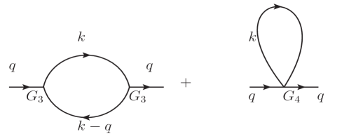
Figure 4: Diagrams that contribute at one loop order to the quadratic term (111) in the effective action.

At one loop order and restricting attention to terms quadratic in $\displaystyle\zeta$ we have (see figure 4)

$$\begin{split}&S^{1PI}_{RB}(\zeta)-S^{eff}_{RB}(\zeta)=\frac{1}{2\kappa_{B}^{2}}\int\frac{d^{3}q}{(2\pi)^{3}}\delta\Gamma_{2}(q)\zeta(q)\zeta(-q),\\ &\delta\Gamma_{2}(q)=-\frac{g_{3}^{2}}{2g_{2}^{2}}\int\frac{d^{3}k}{(2\pi)^{3}}\frac{1}{|k||k-q|}-\frac{1}{2g_{2}}\int\frac{d^{3}k}{(2\pi)^{3}}\frac{{\tilde{G}}^{0}_{4}(q,-q,k,-k)}{|k|}.\end{split}$$ (111)

The integral in the first term in the second line of (111) is easily evaluated in dimensional regularization:

$$\int\frac{d^{3}k}{(2\pi)^{3}}\frac{1}{|k||k-q|}=-\frac{|q|}{4\pi^{2}}.$$ (112)

Note in particular that the integral (112) has a linear divergence but not a logarithmic divergence, so it does not contribute to the $\displaystyle\beta$ functions we compute below. The second term on the second line of (111) cannot be evaluated in general, as we do not know the full Green’s function $\displaystyle{\tilde{G}}^{0}_{4}(q,-q,k,-k)$. However logarithmic divergences in this integral at large $\displaystyle k$ can only arise from terms in $\displaystyle{\tilde{G}}^{0}_{4}$ that have the homogeneity of $\displaystyle\frac{|q|}{k^{2}}$. The relevant terms are those proportional to $\displaystyle{\tilde{g}}_{(4,2)}$ and $\displaystyle{\tilde{g}}_{(4,3)}$. Using the fact that $\displaystyle\cos^{2}(\theta)$ averages to $\displaystyle\frac{1}{3}$ on the two-sphere, the divergent part of $\displaystyle\delta\Gamma_{2}$ is

$$\delta\Gamma_{2}(q)=-\left(\frac{{\tilde{g}}_{(4,2)}+\frac{{\tilde{g}}_{(4,3)}}{3}}{2g_{2}}\right)\int\frac{d^{3}k}{(2\pi)^{3}}\frac{|q|}{|k|^{3}}=-\left(\frac{3{\tilde{g}}_{(4,2)}+{\tilde{g}}_{(4,3)}}{12\pi^{2}g_{2}}\right)|q|\ln\left(\frac{\Lambda}{|q|}\right).$$ (113)

Adding this piece to the quadratic part of $\displaystyle S^{eff}_{RB}(\zeta)$ (see (109)) we conclude that the divergent part of the quadratic terms in the quantum effective action, accurate to one loop, is given by

$$\begin{split}S^{1PI}_{RB}&=\frac{g_{2}}{2\kappa_{B}}\int\frac{d^{3}q}{(2\pi)^{3}}|q|\left(\frac{|q|}{\Lambda}\right)^{\frac{2\delta^{\prime}_{B}(\lambda_{B})}{\kappa_{B}}}\zeta(q)\zeta(-q),\\ 2\delta^{\prime}_{B}(\lambda_{B})&=2\delta_{B}+\frac{3{\tilde{g}}_{(4,2)}+{\tilde{g}}_{(4,3)}}{12\pi^{2}g_{2}^{2}}.\\ \end{split}$$ (114)

Using

$$\frac{3{\tilde{g}}_{(4,2)}+{\tilde{g}}_{(4,3)}}{12\pi^{2}g_{2}^{2}}=\frac{32}{3\pi\sin\pi\lambda_{B}}$$ (115)

we conclude that

$$\delta_{B}^{\prime}-\delta_{B}=\frac{16}{3\pi\sin\pi\lambda_{B}}$$ (116)

Note that (114) implies that

$$\langle\zeta(p)\zeta(-p^{\prime})\rangle\propto(2\pi)^{3}\delta^{3}(p-p^{\prime})\frac{1}{|q|^{1+2\delta^{\prime}_{B}/\kappa_{B}}}.$$ (117)

It follows that the scaling dimension of $\displaystyle\zeta$, $\displaystyle\Delta_{\zeta}$, is given by

$$\Delta_{\zeta}=1-\frac{\delta^{\prime}_{B}}{\kappa_{B}}.$$ (118)

Recall on the other hand that

$$\Delta_{\sigma}=2+\frac{\delta_{B}}{\kappa_{B}}.$$ (119)

The formula (116) thus asserts that at order $\displaystyle\frac{1}{N}$, the difference between minus of the anomalous dimension of the (approximately) dimension one operator of the regular boson theory and the anomalous dimension of the (approximately) dimension 2 operator of the critical boson theory is given by $\displaystyle\frac{32}{3\pi^{2}{\tilde{N}}}$ (where the quantity $\displaystyle{\tilde{N}}$ is the abstract parameter in terms of which the authors of Maldacena:2012sf determined three point functions of the theory). It is possible that this elegant formula has a simple explanation.

3.5.2 Check at small $\displaystyle\lambda_{B}$

As a check of our formulae we now use (114) to compute $\displaystyle\delta^{\prime}_{B}$ in the limits $\displaystyle\lambda_{B}\to 0$ and $\displaystyle\lambda_{F}\to 0$.

In the limit $\displaystyle\lambda_{B}=0$ explicit computations yield (see (36) and (17))

$$\delta_{B}=-\frac{16}{3\pi^{2}\lambda_{B}},\qquad$$ (120)

It follows from (116) that $\displaystyle\delta_{B}^{\prime}=0$. The fact that $\displaystyle\delta_{B}^{\prime}$ vanishes at $\displaystyle\lambda_{B}=0$ is a consistency check of our formalism, as the regular boson theory is free when $\displaystyle\lambda_{B}=0$ (and when $\displaystyle g_{3}$ also vanishes).

3.5.3 Check at small $\displaystyle\lambda_{F}$

Recall that the regular fermion theory is free at $\displaystyle\lambda_{F}=0$; it thus follows that $\displaystyle\delta_{B}=0$ when $\displaystyle\lambda_{F}=0$. (116) then implies that

$$\delta^{\prime}_{B}=-\frac{16}{3\pi^{2}\lambda_{F}}.$$ (121)

In other words (see (118)) the dimension of the approximately dimension one operator in the ungauged 3d Gross-Neveu model is predicted by (116) to be

$$\Delta_{\zeta}=1+\frac{16}{3\pi^{2}\lambda_{F}\kappa_{B}}=1-\frac{16}{3\pi^{2}N_{F}},$$ (122)

where we have used $\displaystyle\kappa_{F}=-\kappa_{B}$. The prediction (122) is correct; it matches the anomalous dimension independently computed in, for example, Giombi:2016zwa and references therein.

3.5.4 $\displaystyle SO(N)$ theory

As we have already noted, at leading order in the large $\displaystyle N$ limit $\displaystyle S^{eff}_{SO(N)}(\zeta)=\frac{1}{2}S^{eff}_{SU(N)}(\zeta)$, which implies that to get $\displaystyle S^{eff}_{SO(N)}$ we need to take

$$g_{i}\rightarrow\frac{1}{2}g_{i}~{}~{}{\rm{for}}~{}i=2,3,4,\cdots.$$ (123)

For the $\displaystyle SO(N)$ theory the anomalous dimension of $\displaystyle\zeta$ that follows from this is (114)

$$\begin{split}2\delta^{{}^{\prime},SO(N)}_{B}(\lambda_{B})=2\delta_{B}^{SO(N)}+2\left(\frac{3{\tilde{g}}_{(4,2)}+{\tilde{g}}_{(4,3)}}{12\pi^{2}g_{2}^{2}}\right).\\ \end{split}$$ (124)

Recall that $\displaystyle\delta_{B}^{SO(N)}=2\delta_{B}^{SU(N)}$, and thus it follows that

$$\delta^{{}^{\prime},SO(N)}_{B}=2\delta^{{}^{\prime},SU(N)}_{B},$$ (125)

hence the anomalous dimension of $\displaystyle\zeta$ in the $\displaystyle SO(N)$ theory is twice that of the $\displaystyle SU(N)$ theory.

It follows that for the $\displaystyle SO(N_{F})$ theory

$$\Delta_{\zeta}=1-\frac{32}{3\pi^{2}N_{F}}.$$ (126)

(126) agrees with the anomalous dimension of $\displaystyle\zeta$ in the $\displaystyle SO(N_{F})$ critical fermion theory at $\displaystyle\lambda_{F}=0$ (see e.g. equation (3.12) in Giombi:2017rhm ).

3.5.5 Computation of $\displaystyle S^{1PI}_{RB}(\zeta)-S^{eff}_{RB}(\zeta)$ at cubic order

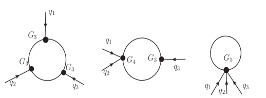
Figure 5: Diagrams that contribute to the one-loop correction (127) to the effective action.

The diagrams that contribute to the one loop renormalization of the cubic part of the effective action are depicted in Figure 5. Evaluating these diagrams we find

$$\begin{split}S^{1PI}_{RB}(\zeta)-S^{eff}_{RB}(\zeta)&=\frac{1}{6\kappa_{B}^{3}}\int\left(\prod_{i}\frac{d^{3}q_{i}}{(2\pi)^{3}}\right)\delta\Gamma_{3}(q_{1},q_{2},q_{3})(2\pi)^{3}\delta(q_{1}+q_{2}+q_{3})\zeta(q_{1})\zeta(q_{2})\zeta(q_{3})\\ \delta\Gamma_{3}(q_{1},q_{2},q_{3})&=\int\frac{d^{3}q}{(2\pi)^{3}}\frac{G_{3}^{S}(q_{1},q,-q-q_{1})G_{3}^{S}(q_{2},-q+q_{3},q+q_{1})G_{3}^{S}(q_{3},-q,q-q_{3})}{G_{2}^{0}(q+q_{1})G_{2}^{0}(q-q_{3})G_{2}(q)}\\ &\qquad-\frac{3}{2}\int\frac{d^{3}q}{(2\pi)^{3}}\frac{{\tilde{G}}_{4}^{0}(q_{1},q_{2},-q+q_{3},q)G_{3}^{S}(q-q_{3},-q,q_{3})}{G_{2}^{0}(q)G_{2}^{0}(q-q_{3})}\\ &\qquad+\frac{1}{2}\int\frac{d^{3}q}{(2\pi)^{3}}\frac{{\tilde{G}}_{5}^{0}(q_{1},q_{2},q_{3},q,-q)}{G_{2}^{0}(q)}\\ &=\frac{g_{3}^{3}}{g_{2}^{3}}\int\frac{d^{3}q}{(2\pi)^{3}}\frac{1}{|q||q-q_{3}||q+q_{1}|}+\\ &\qquad\frac{3g_{3}}{2g_{2}^{2}}\int\frac{d^{3}q}{(2\pi)^{3}}\frac{{\tilde{G}}^{0}_{4}(q_{1},q_{2},q,q_{3}-q)}{|q_{3}-q||q|}-\frac{1}{2g_{2}}\int\frac{d^{3}q}{(2\pi)^{3}}\frac{{\tilde{G}}^{0}_{5}(q,-q,0,0,0)}{|q|}\\ &\simeq\frac{1}{2\pi^{2}}\left(\frac{g_{3}^{3}}{g_{2}^{3}}+\frac{3g_{3}{\tilde{g}}_{(4,1)}}{2g_{2}^{2}}-\frac{{\tilde{g}}_{(5,0)}}{2g_{2}}\right)\ln(\Lambda),\\ G_{3}^{S}(q_{1},q_{2},q_{3})&\equiv-\frac{g_{3}}{6\kappa_{B}^{2}}(2\pi)^{3}\delta(q_{1}+q_{2}+q_{3}),\\ \end{split}$$ (127)

where $\displaystyle g_{3}$ was listed in (110) and where we have retained only divergent terms. It follows that the one loop corrected cubic term in the quantum effective action relevant for the computation of the $\displaystyle\beta$ function is given by

$$\begin{split}S^{1PI}_{RB}&=\frac{g^{\prime}_{3}}{6\kappa_{B}^{2}}\int\frac{d^{3}q_{1}}{(2\pi)^{3}}\frac{d^{3}q_{2}}{(2\pi)^{3}}\frac{d^{3}q_{3}}{(2\pi)^{3}}(2\pi)^{3}\delta(q_{1}+q_{2}+q_{3})\zeta(q_{1})\zeta(q_{2})\zeta(q_{3}),\\ g^{\prime}_{3}&=g_{3}+\frac{1}{2\pi^{2}\kappa_{B}}\left(2\pi^{2}\text{sgn}(\kappa_{B})\delta_{B}{\tilde{g}}_{3}+\frac{g_{3}^{3}}{g_{2}^{3}}+\frac{3g_{3}{\tilde{g}}_{(4,1)}}{2g_{2}^{2}}-\frac{{\tilde{g}}_{(5,0)}}{2g_{2}}\right)\ln(\Lambda).\end{split}$$ (128)

3.6 The $\displaystyle\beta$ function for $\displaystyle x_{6}$ at first subleading order in $\displaystyle\frac{1}{N_{B}}$

Keeping track only of those one loop corrections that scale like $\displaystyle\ln(\Lambda)$, and truncating to quadratic and cubic order in $\displaystyle\zeta$, we have

$$\begin{split}S^{1PI}_{RB}&=\frac{g_{2}}{2\kappa_{B}}\int\frac{d^{3}q}{(2\pi)^{3}}\frac{|q|^{1+2\frac{\delta^{\prime}_{B}}{\kappa_{B}}}}{\Lambda^{2\frac{\delta^{\prime}_{B}}{\kappa_{B}}}}\zeta(q)\zeta(-q)\\ &\quad+\frac{g^{\prime}_{3}}{6\kappa_{B}^{2}}\int\frac{d^{3}q_{1}}{(2\pi)^{3}}\frac{d^{3}q_{2}}{(2\pi)^{3}}\frac{d^{3}q_{3}}{(2\pi)^{3}}(2\pi)^{3}\delta(q_{1}+q_{2}+q_{3})\zeta(q_{1})\zeta(q_{2})\zeta(q_{3}).\\ \end{split}$$ (129)

The variable change

$${\tilde{\zeta}}=\frac{\zeta}{\Lambda^{\frac{\delta^{\prime}_{B}}{\kappa_{B}}}}$$ (130)

allows us to eliminate $\displaystyle\Lambda$ from the quadratic part of the action. In terms of the new variable we have

$$\begin{split}S^{1PI}_{RB}&=\frac{g_{2}}{2\kappa_{B}}\int\frac{d^{3}q}{(2\pi)^{3}}{|q|^{1+2\frac{\delta^{\prime}_{B}}{\kappa_{B}}}}{\tilde{\zeta}}(q){\tilde{\zeta}}(-q)\\ &+\frac{g^{\prime\prime}_{3}}{6\kappa_{B}^{2}}\int\frac{d^{3}q_{1}}{(2\pi)^{3}}\frac{d^{3}q_{2}}{(2\pi)^{3}}\frac{d^{3}q_{3}}{(2\pi)^{3}}(2\pi)^{3}\delta(q_{1}+q_{2}+q_{3}){\tilde{\zeta}}(q_{1}){\tilde{\zeta}}(q_{2}){\tilde{\zeta}}(q_{3}),\\ 2\delta^{\prime}_{B}&=2\delta_{B}+\frac{3{\tilde{g}}_{(4,2)}+{\tilde{g}}_{(4,3)}}{12\pi^{2}g_{2}^{2}},\\ g^{\prime\prime}_{3}&=g_{3}^{\prime}\Lambda^{\frac{3\delta_{B}^{\prime}}{\kappa_{B}}}=g_{3}+\left(\frac{{\tilde{g}}_{3}\delta_{B}}{\kappa_{B}}+g_{3}\left(\frac{3{\tilde{g}}_{(4,1)}}{4\pi^{2}\kappa_{B}g_{2}^{2}}+\frac{3\delta_{B}^{\prime}}{\kappa_{B}}\right)+g_{3}^{3}\left(\frac{1}{2\pi^{2}\kappa_{B}g_{2}^{3}}\right)-\frac{{\tilde{g}}_{(5,0)}}{4\pi^{2}\kappa_{B}g_{2}}\right)\ln(\Lambda).\end{split}$$ (131)

It follows that the dynamics defined by the action (131) is independent of the cutoff scale $\displaystyle\Lambda$ if and only if

$$\begin{split}\frac{dg_{3}}{d\ln(\Lambda)}&=(24\pi^{2})\frac{dx_{6}^{B,F}}{d\ln(\Lambda)}=(24\pi^{2})\beta,\\ (24\pi^{2})\beta&=\left(\frac{{\tilde{g}}_{(5,0)}}{4\pi^{2}\kappa_{B}g_{2}}-\frac{{\tilde{g}}_{3}\delta_{B}}{\kappa_{B}}\right)-g_{3}\left(\frac{3{\tilde{g}}_{(4,1)}}{4\pi^{2}\kappa_{B}g_{2}^{2}}+\frac{3\delta_{B}^{\prime}}{\kappa_{B}}\right)-g_{3}^{3}\left(\frac{1}{2\pi^{2}\kappa_{B}g_{2}^{3}}\right),\\ \end{split}$$ (132)

where in the first line we used (110).

(132) is the beta function of the $\displaystyle SU(N)$ theory. Using the reasoning outlined in subsubsection 3.5.4 it follows that the $\displaystyle\beta$ function of the $\displaystyle SO(N)$ theory is given by

$$\begin{split}\frac{1}{2}\frac{dg_{3}}{d\ln(\Lambda)}&=\frac{(24\pi^{2})}{2}\frac{dx_{6}^{B,F}}{d\ln(\Lambda)}=\left(\frac{{\tilde{g}}_{(5,0)}}{4\pi^{2}\kappa_{B}g_{2}}-\frac{{\tilde{g}}_{3}\delta_{B}}{\kappa_{B}}\right)-g_{3}\left(\frac{3{\tilde{g}}_{(4,1)}}{4\pi^{2}\kappa_{B}g_{2}^{2}}+\frac{3\delta_{B}^{\prime}}{\kappa_{B}}\right)-g_{3}^{3}\left(\frac{1}{2\pi^{2}\kappa_{B}g_{2}^{3}}\right).\\ \end{split}$$ (133)

In other words, the beta function of $\displaystyle x_{6}$ in $\displaystyle SO(N)$ is exactly twice the $\displaystyle\beta$ function for $\displaystyle x_{6}$ in the $\displaystyle SU(N)$ theory.

In summary, the $\displaystyle SU(N)$ beta function listed in (132) is a cubic polynomial of the form

$$\beta(g_{3})=-a+bg_{3}-cg_{3}^{3},$$ (134)

with coefficients that are functions of $\displaystyle\lambda$, given by

$$\begin{split}a&=-\left(\frac{{\tilde{g}}_{(5,0)}}{4\pi^{2}\kappa_{B}g_{2}}-\frac{{\tilde{g}}_{3}\delta_{B}}{\kappa_{B}}\right),\\ b&=-\left(\frac{3{\tilde{g}}_{(4,1)}}{4\pi^{2}\kappa_{B}g_{2}^{2}}+\frac{3\delta_{B}^{\prime}}{\kappa_{B}}\right),\\ c&=\left(\frac{1}{2\pi^{2}\kappa_{B}g_{2}^{3}}\right),\\ g_{3}&=(24\pi^{2})\left(x_{6}^{B}-\frac{4}{3}\cot^{2}\left(\frac{\pi\lambda_{B}}{2}\right)\right)=(24\pi^{2})\left(x_{6}^{F}-\frac{4}{3}\tan^{2}\left(\frac{\pi\lambda_{F}}{2}\right)\right).\\ \end{split}$$ (135)

(135) is one of the central results of this paper. Recall that $\displaystyle g_{2}$ and $\displaystyle{\tilde{g}}_{(4,1)}$ are both known functions of $\displaystyle\lambda_{B}$ (both are listed in (110)). The quantity $\displaystyle{\tilde{g}}_{(5,0)}$ characterizes a particular kinematical limit of the leading large $\displaystyle N_{B}$ five point function of $\displaystyle{\tilde{J}}_{0}$ operators (see (110) for a precise definition). This quantity is currently not known as a function of $\displaystyle\lambda_{B}$ (but may well be possible to evaluate in the near future using the techniques of Yacoby:2018yvy ). The quantity $\displaystyle\delta_{B}$ parameterizes the anomalous dimension of $\displaystyle{\tilde{J}}_{0}$ at first subleading order in $\displaystyle\frac{1}{N_{B}}$. It is precisely defined in (16), and is currently not known as a function of $\displaystyle\lambda_{B}$. The quantity $\displaystyle{\tilde{g}}_{3}$ parameterizes the split of the three point function of three $\displaystyle{\tilde{J}}_{0}$ operators into contact and non-contact pieces and was precisely defined in (110) and (LABEL:thptdet). This quantity is also currently not known as a function of $\displaystyle\lambda_{B}$. Finally $\displaystyle\delta^{\prime}_{B}$ is given in terms of $\displaystyle\delta_{B}$ by (116).

In the rest of this section we will first study the behaviour of the beta function (134) and (135) in the small $\displaystyle\lambda_{B}$ and $\displaystyle\lambda_{F}$ limits, and then study the global properties of the flows described by (134).

3.7 The limit $\displaystyle\lambda_{B}\to 0$

To analyze the $\displaystyle\lambda_{B}\to 0$ limit, we introduce a rescaled coupling $\displaystyle\lambda_{6}$ defined by

$$x_{6}^{B}=\frac{\lambda_{6}}{\lambda_{B}^{2}},$$ (136)

and work at fixed $\displaystyle\lambda_{6}$ in the limit $\displaystyle\lambda_{B}\to 0$. In this limit the regular boson action (95) simplifies to

$$S_{RB}(\phi)=\int d^{3}x\left(D_{\mu}\bar{\phi}D^{\mu}\phi+\frac{(2\pi)^{2}}{N_{B}^{2}}\lambda_{6}(\bar{\phi}\phi)^{3}\right).$$ (137)

Plugging (36) into (132), using the fact that $\displaystyle\delta_{B}=0$, and using the results of Appendix B.2.3 we find

$$\frac{d\lambda_{6}}{d\ln(\Lambda)}=\frac{1}{N_{B}}9\lambda_{6}^{2}\left(1-\frac{\pi^{2}}{16}\lambda_{6}\right).$$ (138)

Similarly, if we plug (136) into the action for the $\displaystyle SO(N)$ regular boson theory we obtain the action

$$S=\int d^{3}x\left(\frac{1}{2}\partial_{\mu}\phi\partial^{\mu}\phi+\frac{(2\pi)^{2}}{2N_{B}^{2}}\lambda_{6}\phi^{6}\right)$$ (139)

(note that $\displaystyle\phi$ are now real fields). The beta function for this theory is simply twice (138), i.e.

$$\frac{1}{2}\frac{d\lambda_{6}}{d\ln(\Lambda)}=\frac{1}{N_{B}}9\lambda_{6}^{2}\left(1-\frac{\pi^{2}}{16}\lambda_{6}\right).$$ (140)

Let us now compare the beta function in (140) with the beta function reported in Pisarski:1982vz . The action in Pisarski:1982vz is given by

$$S=\int d^{3}x\left(\frac{1}{2}\partial_{\mu}\phi\partial^{\mu}\phi+\frac{\pi^{2}}{3}\lambda_{6}^{Pisarski}\phi^{6}\right),$$ (141)

which matches with (137) if we make the identification

$$\lambda_{6}^{our}=\frac{N_{B}^{2}}{6}\lambda_{6}^{Pisarski}.$$ (142)

In Pisarski:1982vz the leading order in large $\displaystyle N_{B}$ beta function is given by

$$\frac{d\lambda_{6}^{Pisarski}}{d\ln(\Lambda)}=3N_{B}(\lambda_{6}^{Pisarski})^{2}-N_{B}^{3}\frac{\pi^{2}}{32}(\lambda_{6}^{Pisarski})^{3}.$$ (143)

It is easy to check that (140) reduces to (143) with the identification (142), showing the consistency of our beta function with that of Pisarski:1982vz .

3.8 Flows at order $\displaystyle\lambda_{B}^{2}$

In Aharony:2011jz the $\displaystyle SO(N_{B})$ regular boson theory was studied in the perturbative regime, i.e. with $\displaystyle\lambda_{B}$ and $\displaystyle\lambda_{6}$ both small, and with $\displaystyle\lambda_{6}\sim\lambda_{B}^{2}$. The variables used in Aharony:2011jz differ from those we have used in their normalization; the translation dictionary is given by

$$\begin{split}\lambda_{6}^{there}&=96\pi^{2}\lambda_{6},\\ \lambda^{there}&=4\pi^{2}\lambda_{B}.\end{split}$$ (144)

The $\displaystyle\beta$ function reported in Aharony:2011jz is

$$\frac{d\lambda_{6}^{there}}{d\ln(\Lambda)}=\frac{1}{N_{B}}\left(\frac{33(N_{B}-1)}{32N_{B}\pi^{2}}(\lambda^{there})^{4}-\frac{5(N_{B}-1)}{4N_{B}\pi^{2}}(\lambda^{there})^{2}~{}\lambda_{6}^{there}+\frac{3N_{B}+22}{16N_{B}\pi^{2}}(\lambda_{6}^{there})^{2}\right).$$ (145)

Using (144), (145) turns into

$$\frac{d\lambda_{6}}{d\ln(\Lambda)}=\frac{1}{N_{B}}\left(\frac{11(1-\frac{1}{N_{B}})}{4}\lambda_{B}^{4}-20(1-\frac{1}{N_{B}})\lambda_{B}^{2}~{}\lambda_{6}+\left(18+\frac{198}{N_{B}}\right)\lambda_{6}^{2}\right).$$ (146)

The results presented in this subsection so far apply at all values of $\displaystyle N_{B}$. Specializing to the large $\displaystyle N_{B}$ limit we obtain

$$\frac{d\lambda_{6}}{d\ln(\Lambda)}=\frac{1}{N_{B}}\left(\frac{11}{4}\lambda_{B}^{4}-20\lambda_{B}^{2}~{}\lambda_{6}+18\lambda_{6}^{2}\right)$$ (147)

for the $\displaystyle SO(N_{B})$ theory, and

$$2\frac{d\lambda_{6}}{d\ln(\Lambda)}=\frac{1}{N_{B}}\left(\frac{11}{4}\lambda_{B}^{4}-20\lambda_{B}^{2}~{}\lambda_{6}+18\lambda_{6}^{2}\right)$$ (148)

for the $\displaystyle SU(N_{B})$ theory. Note that the first term on the right-hand side of (140) agrees with the last term on the right-hand side of (147), establishing the consistency between these two formulae.

(148) carries qualitatively important information as we now explain. The beta function (138) has a zero $\displaystyle\lambda_{6}=\frac{16}{\pi^{2}}$ together with a double zero at $\displaystyle\lambda_{6}=0$. The zero at $\displaystyle\lambda_{6}=\frac{16}{\pi^{2}}$ is robust; small $\displaystyle\lambda_{B}$ corrections will change the precise value of the zero but cannot destabilize it. On the other hand a double zero is unstable to small corrections; corrections of one sign could cause the double zero to split into two single zeroes, while the opposite correction could remove the zeroes altogether. It is easy to check that the corrections (147) split the double zero into two single zeroes located (for large $\displaystyle N_{B}$) at

$$\lambda_{6}=\frac{20\pm\sqrt{202}}{36}\lambda_{B}^{2},$$ (149)

or

$$x_{6}+1=\frac{20\pm\sqrt{202}}{36}.$$ (150)

The larger of the two roots (the attractive fixed point in the sense of flow to the IR) is at

$$x_{6}+1=.95035\cdots,$$ (151)

while the smaller root (the repulsive fixed point in the sense of flow towards the IR) lies at

$$x_{6}+1=.16076\cdots.$$ (152)

It follows that at small $\displaystyle\lambda_{B}$ the approximate domain of attraction of the attractive fixed point is the large range

$$x_{6}+1\in(.16076,\frac{16}{\pi^{2}\lambda_{B}^{2}}).$$ (153)

3.9 The limit $\displaystyle\lambda_{F}\to 0$

As we have seen above, in the limit $\displaystyle\lambda_{F}\to 0$

$$\delta^{\prime}_{B}(\lambda_{F})=-\frac{16}{3\pi^{2}\lambda_{F}}.$$ (154)

We now turn to the $\displaystyle\beta$ function in this limit. Plugging (154), (345) and (56) into (132) we obtain

$$\begin{split}\frac{dx_{6}}{d\ln(\Lambda)}&=\frac{32x_{6}}{\kappa_{F}\pi^{2}\lambda_{F}}-\frac{36x_{6}^{3}}{\kappa_{F}\pi^{4}\lambda_{F}^{3}}.\end{split}$$ (155)

The $\displaystyle\beta$ function (155) can be rewritten in terms of the variable $\displaystyle\lambda_{6}^{F}$

$$\lambda_{6}^{F}=\frac{x_{6}}{\lambda_{F}},$$ (156)

in which it has a finite $\displaystyle\lambda_{F}\to 0$ limit

$$\frac{d\lambda^{F}_{6}}{d\ln(\Lambda)}=\frac{1}{N_{F}}\left(\frac{32\lambda_{6}^{F}}{\pi^{2}}-\frac{36\left(\lambda_{6}^{F}\right)^{3}}{\pi^{4}}\right).$$ (157)

The zeros of this beta function occur at $\displaystyle\lambda_{6}^{F}=0$ and $\displaystyle\lambda_{6}^{F}=\pm\frac{2\sqrt{2}\pi}{3}$, or at

$$x_{6}=\left(0,\pm\frac{2\sqrt{2}\pi\lambda_{F}}{3}\right).$$ (158)

Notice that all three zeroes of this beta function are of order $\displaystyle\lambda_{F}$.

The scalings in (157) - and in particular the emergence of the natural variable $\displaystyle\lambda_{6}^{F}$ in the limit $\displaystyle\lambda_{F}\to 0$ is easy to understand. Recall that the critical fermion theory is defined by the action

$$S_{CF}(\psi,\zeta)=S_{RF}(\psi)-\int\frac{4\pi{\bar{\psi}}{\psi}}{{\tilde{\kappa}}_{F}}\zeta(x)+\frac{(2\pi)^{2}}{{\tilde{\kappa}}_{F}^{2}}x_{6}\int\zeta^{3}(x).$$ (159)

The variable change

$$\zeta=-\frac{{\tilde{\kappa}}_{F}}{4\pi}\sigma_{F}$$ (160)

recasts this Lagrangian into the form

$$S_{CF}(\psi,\zeta)=S_{RF}(\psi)+\int{\bar{\psi}}{\psi}\sigma_{F}-\frac{N_{F}\lambda_{6}^{F}}{8\pi}\int\sigma_{F}^{3}(x),$$ (161)

which has a finite limit as $\displaystyle{\tilde{\kappa}}_{F}\to\infty$, explaining the structure of (157).

The theory (161) with $\displaystyle\lambda_{F}=\lambda_{6}^{F}=0$ has a parity symmetry, under which $\displaystyle\sigma_{F}$ is odd. This implies that both $\displaystyle\lambda_{F}$ and $\displaystyle\lambda_{6}^{F}$ change sign under a parity transformation. This is consistent with the form of (157), and implies that at weak coupling $\displaystyle\lambda_{6}^{F}=0$ must be a fixed point, and that the two other zeroes have equal magnitude and opposite sign, as we find.

3.10 Global structure of the flows

Let us now study the properties of the flows described by equation (134) at general values of $\displaystyle\lambda_{B}$ (or $\displaystyle\lambda_{F}$). We first note that the coefficient $\displaystyle c$ in (134) is positive at every value of $\displaystyle\lambda_{B}$ . It follows that $\displaystyle\beta$ is negative at large positive values of $\displaystyle g_{3}$, but positive at large negative values of $\displaystyle g_{3}$. In other words all flows are repulsive at large values of $\displaystyle|g_{3}|$, i.e. flows that start at large positive $\displaystyle g_{3}$ (or equivalently $\displaystyle x_{6}$) end up (in the deep IR) at $\displaystyle g_{3}=\infty$ (equivalently $\displaystyle x_{6}=\infty$). Similarly flows that start out at large negative values of $\displaystyle g_{3}$ (equivalently $\displaystyle x_{6}$) end up at $\displaystyle x_{6}=-\infty$.

The polynomial (134) has exactly one real root whenever

$$27a^{2}c>4b^{3},$$ (162)

and in this case the fixed point is repulsive (UV-stable). On the other hand it has three real roots when

$$27a^{2}c<4b^{3}.$$ (163)

At the boundary between these two regimes there is one double zero at

$$g_{3}=\sqrt{\frac{b}{2c}},$$ (164)

and one additional root.

When the condition (163) is satisfied, the outer two roots are repulsive (in the sense of flow towards the IR) and represent fixed points about which $\displaystyle\zeta^{3}$ is a relevant operator. However the middle root is attractive, and represents a fixed point about which $\displaystyle\zeta^{3}$ is an irrelevant operator.

Near $\displaystyle\lambda_{B}=0$ we have

$$a=-\frac{4096}{\kappa_{B}\pi^{2}\lambda_{B}^{3}},~{}~{}~{}b=\frac{48}{\kappa_{B}\pi^{2}\lambda_{B}},~{}~{}~{}c=\frac{\lambda_{B}^{3}}{1024\pi^{2}\kappa_{B}},~{}~{}~{}$$ (165)

and $\displaystyle 27a^{2}c=4b^{3}$, so we are at the boundary between the cases (162) and (163). The beta function has a double root at

$$g_{3}=-\frac{128}{\lambda_{B}^{2}},$$ (166)

i.e. at $\displaystyle\lambda_{6}=0$, and a single root at

$$g_{3}=\frac{256}{\lambda_{B}^{2}},$$ (167)

i.e. at

$$\lambda_{6}=\frac{16}{\pi^{2}},$$ (168)

in agreement with (138). Turning on a small Chern-Simons coupling $\displaystyle\lambda_{B}$ takes us into the regime (163). As described above, the double root of the $\displaystyle\lambda_{B}=0$ theory splits into two roots, one repulsive and one attractive. The domain of attraction of the attractive root is listed in (153) and becomes large as $\displaystyle\lambda_{B}\to 0$.

In the opposite limit $\displaystyle\lambda_{F}=0$ we have $\displaystyle a=0$ with $\displaystyle b$ and $\displaystyle c$ positive, so we lie squarely within the regime of (163). Once again we have two repulsive roots and one attractive root. The domain of attraction of the attractive root is the interval

$$x_{6}\in(-\lambda_{F}\sqrt{\frac{2}{3\pi^{2}}},\lambda_{F}\sqrt{\frac{2}{3\pi^{2}}}),$$ (169)

which becomes very small as $\displaystyle\lambda_{F}\to 0$.

At general values of $\displaystyle\lambda_{B}$ the coefficient $\displaystyle c(\lambda_{B})$ is given by (135) and (110). It follows from these exact results that $\displaystyle|\kappa_{B}|c$ is an even function of $\displaystyle\lambda_{B}$. This function starts out at zero when $\displaystyle\lambda_{B}=0$ and then increases monotonically with $\displaystyle\lambda_{B}$, reaching infinity as $\displaystyle\lambda_{B}$ approaches unity. As we have mentioned above, $\displaystyle c$ is positive at every value of $\displaystyle\lambda_{B}$.

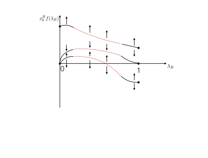
Figure 6: A schematic description of the large $\displaystyle N$ RG flows towards low energies described in section 3.10. The vertical axis is $\displaystyle x_{6}$ multiplied by a convenient function of $\displaystyle\lambda$, that keeps the fixed points at a finite separation both as $\displaystyle\lambda_{B}\to 0$ and as $\displaystyle\lambda_{F}\to 0$. The flows near the two limiting values of $\displaystyle\lambda_{B}$ (with the fixed points depicted as solid lines) are based on computations, while the flows in the middle (with the fixed points depicted as dashed lines) are conjectured, and it is possible that two of the lines actually meet and disappear for some value of $\displaystyle\lambda_{B}$ and then reappear at a larger value.

$\displaystyle|\kappa_{B}|a$ starts out at $\displaystyle-\infty$ at $\displaystyle\lambda_{B}=0$ but vanishes at $\displaystyle\lambda_{B}=1$ (the vanishing is a direct consequence of the parity transformation properties of the free fermion theory). We do not know the value of $\displaystyle a$ at intermediate values of $\displaystyle\lambda_{B}$. The simplest possibility is that $\displaystyle a$, like $\displaystyle c$, increases monotonically as a function of $\displaystyle\lambda_{B}$, and in particular is always negative.

$\displaystyle|\kappa_{B}|b$ starts out at $\displaystyle\infty$ at $\displaystyle\lambda_{B}=0$ and then decreases like $\displaystyle\frac{1}{\lambda_{B}}$ as $\displaystyle\lambda_{B}$ is increased. Near $\displaystyle\lambda_{B}=1$ this function once again blows up in a manner proportional to $\displaystyle\frac{1}{1-\lambda_{B}}$. We do not know the detailed functional form of $\displaystyle b$ at intermediate values of $\displaystyle\lambda_{B}$. The simplest possibility consistent with these boundary conditions is that $\displaystyle|\kappa_{B}|b$ monotonically decreases from $\displaystyle\lambda_{B}=0$ to some $\displaystyle\lambda_{B}=\lambda_{min}$, after which it monotonically increases as $\displaystyle\lambda_{B}$ is increased from $\displaystyle\lambda_{min}$ to unity.

As we have explained above, the global structure of the $\displaystyle\beta$ function is really determined by the ratio $\displaystyle\frac{27a^{2}c}{b^{3}}$. This ratio starts out at unity at $\displaystyle\lambda_{B}=0$, decreases as $\displaystyle\lambda_{B}$ is increased away from zero and reaches the value zero when $\displaystyle\lambda_{B}=1$. We do not know the detailed functional form of this ratio as a function of $\displaystyle\lambda_{B}$. The simplest possibility is that this function decreases monotonically as a function of $\displaystyle\lambda_{B}$ as $\displaystyle\lambda_{B}$ is varied from $\displaystyle 0$ to unity. If this possibility is realized then the RG flows described in this paper have two repulsive and one attractive fixed point at every value of $\displaystyle\lambda_{B}$ (see Figure 6 for a schematic description). Note that the size of the domain of attraction of this central stable fixed point (measured as the size of the interval of the variable $\displaystyle x_{6}$) is very large at small $\displaystyle\lambda_{B}$ but goes to zero as $\displaystyle\lambda_{B}\to 1$.

3.11 Relevant deformations, thermodynamics and duality

So far in this section we have intensively studied RG flows of the parameter $\displaystyle x_{6}$. $\displaystyle x_{6}$ is special because the operator it multiplies, $\displaystyle\zeta^{3}$, is marginal in the large $\displaystyle N$ limit. As a consequence, flows of $\displaystyle x_{6}$ are controlled by a beta function of order $\displaystyle\frac{1}{N}$ and so are very slow, as we have seen earlier in this section.

In contrast to $\displaystyle\zeta^{3}$, the operators $\displaystyle\zeta^{2}$ and $\displaystyle\zeta$ are relevant even in the strict large $\displaystyle N$ limit. The addition of one of these operators to the regular boson or critical fermion theory results in a ‘fast’ RG flow. These fast flows take place over an ‘RG flow time’ (i.e. logarithm of ratios of scales) of order unity rather than $\displaystyle N$.

Flows induced by $\displaystyle\zeta^{2}$ and $\displaystyle\zeta$ in the large $\displaystyle N$ limit were studied in detail in Jain:2013gza . The qualitative conclusion of this study was the following. A generic deformation in $\displaystyle\zeta^{2},\zeta$ space ends up in a massive theory. A one parameter tuning (tuning the coefficient of $\displaystyle\zeta$ to zero in the dimensional regularization scheme) seeds a flow that ends up (for a specific sign of the $\displaystyle\zeta^{2}$ coefficient) in the CB theory (which by duality is the same as the RF theory) in the IR. The operator $\displaystyle\zeta^{3}$ is irrelevant about the new fixed point, so $\displaystyle x_{6}$ goes to zero and the dynamics of the fixed point is insensitive to the value of $\displaystyle x_{6}$ from which the flow starts.

At a quantitative level, the results described in the previous paragraph were obtained as follows. Consider the $\displaystyle\zeta$ and $\displaystyle\zeta^{2}$ deformed regular boson theory

$$\displaystyle S_{B} \displaystyle=\int d^{3}x\biggl{[}i\varepsilon^{\mu\nu\rho}{\kappa_{B}\over 4\pi}\mathrm{Tr}(A_{\mu}\partial_{\nu}A_{\rho}-{2i\over 3}A_{\mu}A_{\nu}A_{\rho})+i\varepsilon^{\mu\nu\rho}{\kappa_{2}\over 4\pi}B_{\mu}\partial_{\nu}B_{\rho}+D_{\mu}\bar{\phi}D^{\mu}\phi$$

$$\displaystyle~{}~{}~{}~{}~{}~{}~{}~{}~{}~{}~{}~{}~{}+m_{b}^{2}\bar{\phi}\phi+{4\pi b_{4}\over\kappa_{B}}(\bar{\phi}\phi)^{2}+\frac{(2\pi)^{2}}{\kappa_{B}^{2}}\left(x_{6}^{B}+1\right)(\bar{\phi}\phi)^{3}\biggl{]},$$ (170)

and the $\displaystyle\zeta$ and $\displaystyle\zeta^{2}$ deformed critical fermion theory

$$\displaystyle~{}S_{F}= \displaystyle\int d^{3}x\bigg{[}i\varepsilon^{\mu\nu\rho}{\kappa_{F}\over 4\pi}\mathrm{Tr}(A_{\mu}\partial_{\nu}A_{\rho}-{2i\over 3}A_{\mu}A_{\nu}A_{\rho})+i\varepsilon^{\mu\nu\rho}{\kappa_{2}\over 4\pi}B_{\mu}\partial_{\nu}B_{\rho}+\bar{\psi}\gamma_{\mu}D^{\mu}\psi$$

$$\displaystyle~{}~{}~{}~{}~{}~{}~{}~{}~{}~{}~{}~{}~{}-\frac{4\pi}{\kappa_{F}}\zeta(\bar{\psi}\psi-{\kappa_{F}y_{2}^{2}\over 4\pi})-{4\pi y_{4}\over\kappa_{F}}\zeta^{2}+\frac{(2\pi)^{2}}{\kappa_{F}^{2}}x_{6}^{F}\zeta^{3}\bigg{]}.$$ (171)

The finite temperature partition functions of these theories were computed, in the large $\displaystyle N$ limit, in Aharony:2012ns ; Jain:2013py ; Minwalla:2015sca by proceeding along the lines of the discussion of subsection 2.3. In the unHiggsed phase, the free energy for the deformed regular boson turns out to take the form Minwalla:2015sca

$$\begin{split}F_{B}(\rho_{B})&=F_{B,0}+\frac{N_{B}}{6\pi}\Bigg{[}-{\hat{c}}_{B}^{3}+2\left({\hat{c}}_{B}^{2}-{\hat{m}}_{b}^{2}\right){\tilde{\cal S}}+2\lambda_{B}{\hat{b}_{4}}{\tilde{\cal S}}^{2}\\ &-3\int_{-\pi}^{\pi}d\alpha\rho_{B}(\alpha)\int_{{\hat{c}}_{B}}^{\infty}dy~{}y~{}\left(\ln\left(1-e^{-y-i\alpha}\right)+\ln\left(1-e^{-y+i\alpha}\right)\right)\Bigg{]},\end{split}$$ (172)

where $\displaystyle F_{B,0}$ is a constant independent of $\displaystyle{\hat{c}}_{B}$ and the quantity $\displaystyle{\tilde{\cal S}}$ is defined to be the solution to the equation

$$\displaystyle{{\hat{c}}_{B}^{2}} \displaystyle=(4+3x_{6}^{B})\lambda_{B}^{2}{\tilde{\cal S}}^{2}-4\lambda_{B}\hat{b}_{4}{\tilde{\cal S}}+\hat{m}_{b}^{2},$$ (173)

and where $\displaystyle\hat{b}_{4}={b_{4}\over T},\hat{m}_{b}={m_{b}\over T}$, $\displaystyle{\hat{c}}_{B}={c_{B}\over T}$, and $\displaystyle{\hat{c}}_{B,0}=\lim_{T\to 0}{\hat{c}}_{B}$ Minwalla:2015sca . The gap equation that follows from varying (172) takes the form $\displaystyle{\tilde{\cal S}}={\cal S}$ where $\displaystyle{\cal S}$ is defined in (78). It follows in particular that on-shell

$$\displaystyle{{\hat{c}}_{B}^{2}} \displaystyle=(4+3x_{6}^{B})\lambda_{B}^{2}{{\cal S}}^{2}-4\lambda_{B}\hat{b}_{4}{{\cal S}}+\hat{m}_{b}^{2}.$$ (174)

In a soon to appear paper new the regular boson free energy and gap equation have very recently been evaluated in the Higgsed phase as well (using the techniques developed in the recent paper Choudhury:2018iwf ). We refer the reader to new for more details. Here we simply note that the final results of new are in perfect agreement with the predictions of duality, and so can be deduced by applying the duality map to the fermionic results reviewed immediately below, as we will effectively do later in this paper.

The fermionic calculation can be done in two steps. We first integrate out $\displaystyle\psi$ at fixed $\displaystyle\zeta$. If we assume (as we do) that the saddle point value of $\displaystyle\zeta$ is a constant in space time, then the integral over fermions is precisely that performed in section 2. We find the equation

$$\begin{split}F_{F}(\rho_{F})&=\frac{N_{F}}{6\pi}\Bigg{[}{\hat{c}}_{F}^{3}-2\lambda_{F}^{2}{\tilde{\cal C}}^{3}-\frac{3}{2}\left({\hat{c}}_{F}^{2}-\frac{16\pi^{2}}{\kappa_{F}^{2}}{\hat{\zeta}}_{F}^{2}\right){\tilde{\cal C}}+\frac{6\pi{\hat{y}}_{2}^{2}}{\kappa_{F}\lambda_{F}}{\hat{\zeta}}_{F}-\frac{24\pi^{2}{\hat{y}}_{4}}{\kappa_{F}^{2}\lambda_{F}}{\hat{\zeta}}_{F}^{2}+\frac{24\pi^{3}x^{F}_{6}}{\kappa_{F}^{3}\lambda_{F}}{\hat{\zeta}}_{F}^{3}\\ &-3\int_{-\pi}^{\pi}d\alpha\rho_{F}(\alpha)\int_{{\hat{c}}_{F}}^{\infty}dy~{}y~{}\left(\ln\left(1-e^{-y-i\alpha}\right)+\ln\left(1-e^{-y+i\alpha}\right)\right)\Bigg{]},\end{split}$$ (175)

with $\displaystyle{\tilde{\cal C}}$ defined to be the solution to the equation

$${\hat{c}}_{F}^{2}=({2\lambda_{F}}{\tilde{\cal C}}-\frac{4\pi}{\kappa_{F}}\hat{\zeta})^{2},$$ (176)

where $\displaystyle\hat{\zeta}\equiv{\zeta\over T}$, $\displaystyle{\hat{c}}_{F}\equiv{c_{F}\over T}$.

$\displaystyle F_{F}$ in (175) is a function is a function of $\displaystyle{\hat{c}}_{F}$ and $\displaystyle\hat{\zeta}$ and must must be extremized with respect to both of these variables. Extremizing with respect to $\displaystyle{\hat{c}}_{F}$ we get $\displaystyle{\tilde{\cal C}}={{\cal C}}$, or equivalently

$${\hat{c}}_{F}^{2}=({2\lambda_{F}}{{\cal C}}-\frac{4\pi}{\kappa_{F}}\hat{\zeta})^{2},$$ (177)

where $\displaystyle{\cal C}$ is defined in (78). Extremizing with respect to $\displaystyle\hat{\zeta}$ we find

$$\displaystyle-\frac{3}{4}\left(\frac{4\pi}{\kappa_{F}}\right)^{2}\hat{\zeta}^{2}x_{6}^{F}-\frac{16\pi}{\kappa_{F}}\hat{\zeta}\lambda_{F}{\tilde{\cal C}}+\frac{8\pi}{\kappa_{F}}\hat{\zeta}\hat{y}_{4}+4\lambda_{F}^{2}{\tilde{\cal C}}^{2}-\hat{y}_{2}^{2}=0,$$ (178)

where $\displaystyle\hat{y}_{4}={y_{4}\over T},\hat{y}_{2}={y_{2}\over T}$.

The gap equation (177) may be used to evaluate $\displaystyle{\hat{\zeta}}$ in terms of $\displaystyle|{\hat{c}}_{F}|$:

$$\frac{4\pi{\hat{\zeta}}}{\kappa_{F}}=2\lambda_{F}{\cal C}-{\rm sgn}(X)|{\hat{c}}_{F}|,$$ (180)

where

$$X=2\lambda_{F}{\cal C}-\frac{4\pi}{\kappa_{F}}{\hat{\zeta}}.$$ (181)

When

$${\rm sgn}(X)={\rm sgn}(\lambda_{F})$$ (182)

we may use (80) to reexpress (180) as

$$\frac{4\pi{\hat{\zeta}}}{\kappa_{F}}=2\lambda_{B}{\cal S}.$$ (183)

Inserting (183) into (178) and once again using (80) to reexpress all remaining occurrences of $\displaystyle{\cal C}$ in terms of $\displaystyle{\cal S}$ we find that (178) reduces to (174) provided we make the following identifications:

$$\lambda_{F}=\lambda_{B}-{\rm sgn}(\lambda_{B}),\quad x_{6}^{F}=x_{6}^{B},\quad y_{4}=b_{4},\quad y_{2}^{2}=m_{b}^{2}.$$ (184)

It follows that the bosonic and fermionic gap equations have the same solutions if we assume (182). This agreement provides non-trivial support for the conjecture that the RB and CF theories are dual to each other, since they agree also after the relevant deformation. It was demonstrated in Minwalla:2015sca that the agreement between gap equations extends to the off-shell free energies; (175) and (172) are identical with the same identifications, under the assumption that (182) holds.

When

$${\rm sgn}(X)=-{\rm sgn}(\lambda_{F})$$ (185)

we may use (80) to reexpress (180) as

$$\frac{4\pi{\hat{\zeta}}}{\kappa_{F}}=2\lambda_{B}{\cal S}-2|{\hat{c}}_{B}|{\rm sgn}(\lambda_{B}).$$ (186)

Inserting (186) into (178) and once again using (80) to reexpress all remaining occurrences of $\displaystyle{\cal C}$ in terms of $\displaystyle{\cal S}$ and using (184), we find that (178) reduces to

$$3|{\hat{c}}_{B}|^{2}(1+x_{6}^{B})+4b_{4}{\rm sgn}(\lambda_{B})|{\hat{c}}_{B}|+m_{b}^{2}+(4+3x_{6}^{B})\lambda_{B}^{2}{\cal S}^{2}-2\lambda_{B}{\cal S}\left(2b_{4}+|{\hat{c}}_{B}|{\rm sgn}(\lambda_{B})(4+3x_{6}^{B})\right)=0.$$ (187)

(187) is a prediction for the bosonic gap equation in the Higgsed phase. This prediction has been verified in the soon to appear paper new .

We expect the RB (CF) theory to flow to the CB (RF) theory when we turn on $\displaystyle b_{4}>0$ in (170) (or $\displaystyle y_{4}>0$ in (3.11)), and indeed the free energy is consistent with this. Consider the limit

$$x_{6}^{B}=\rm{fixed},~{}\hat{b}_{4}\rightarrow\infty,~{}m_{b}^{2}\rightarrow\infty$$ (188)

with $\displaystyle\frac{m_{b}^{2}}{2b_{4}\lambda_{B}}=m_{B}^{cri}$ fixed. In this limit, (173) is easily solved and yields

$${\tilde{S}}=\frac{m_{B}^{cri}}{2}+\frac{-4c_{B}^{2}+4(m_{B}^{cri})^{3}\lambda_{B}^{3}+3(m_{B}^{cri})^{3}x_{6}\lambda_{B}}{8m_{b}^{2}}+{\cal O}\left(\frac{1}{m_{b}^{4}}\right).$$ (189)

Plugging the solution back into (172) we recover the first equation of (73) (up to $\displaystyle c_{B}$-independent constants), reflecting the fact that the regular boson theory flows to the critical boson theory at low energies, provided we fine-tune so that the pole mass is held fixed. Of course similar results apply to the fermionic theory, and (188) represents a RG flow from the regular boson/critical fermion theories to the critical boson/regular fermion theory. This may be thought of as a derivation of the critical boson-regular fermion duality starting from the conjectured regular boson-critical fermion duality.

Surprisingly, there are also other limits in which the RB (CF) theories seem to flow to the CB (RF) theory, even though $\displaystyle b_{4}=0$ (but $\displaystyle x_{6}$ diverges). We will discuss these limits in section 4.3 below.

4 Phase structure at zero temperature at large $\displaystyle N$

In this section we analyze the large $\displaystyle N$ phase structure of the ‘regular boson’ (or equivalently ‘critical fermion’) theories that are the subject of this paper, at zero temperature (a complete analysis of the phase structure at finite temperature, and especially on $\displaystyle S^{2}\times S^{1}$, would be an interesting but intricate exercise). The ‘critical boson’ (or equivalently ‘regular fermion’) theories have only one relevant deformation (which one can call the fermion mass), and their phase structure is very simple. For either sign of this deformation they flow to a massive theory, which reduces to a topological theory at low energies. In the fermionic $\displaystyle U(N_{F})_{k_{F}}$ theory, for one sign of the mass one obtains the $\displaystyle U(N_{F})_{k_{F}+\frac{1}{2}}$ CS theory, and for the other sign the $\displaystyle U(N_{F})_{k_{F}-\frac{1}{2}}$ CS theory. In the language of the bosonic $\displaystyle U(N_{B})_{k_{B}}$ theory, for one sign one obtains the $\displaystyle U(N_{B})_{k_{B}}$ CS theory, and for the other sign the $\displaystyle U(N_{B}-1)_{k_{B}}$ CS theory, and one interprets this as a Higgsing of the original gauge theory.

The phase structure of the ‘regular boson’ theories is more elaborate, since they have two relevant operators, and another operator that is marginal in the large $\displaystyle N$ limit (and which becomes either relevant or irrelevant at finite $\displaystyle N$, depending on the precise fixed point one discusses). Generic flows from these theories also lead to massive theories, but some special flows lead to the ‘critical boson’ theories. At infinite $\displaystyle N$ the flows are labeled for each $\displaystyle x_{6}$ by the parameters $\displaystyle m_{b}$ and $\displaystyle b_{4}$ in (170), and on dimensional grounds it is clear that the phase structure only depends on the combination $\displaystyle m_{b}^{2}/b_{4}^{2}$, and on the signs of $\displaystyle m_{b}^{2}$ and of $\displaystyle b_{4}$. In certain parameter ranges the gap equations (177) and (178) admit multiple solutions, and then the true phase of the theory is the solution with the lowest free energy. As the parameters of the theory are varied our system can undergo a phase transition of one of two kinds. The first sort of transition occurs when the free energies of two competing branches of solutions can cross. The thermodynamically dominant solution changes discontinuously across such a line, giving rise to a first order phase transition. The second kind of transition happens when the dominant branch of solutions itself changes character across a codimension one wall in parameter space. In this situation we have a second order phase transition, characterized by a conformal field theory, which in our case will always be the ‘critical boson’ theory.

In the zero temperature limit the gap equations and the free energy simplify considerably. Since these equations are invariant under the duality, we can describe them either in the bosonic or in the fermionic language. In this section we will mostly use the bosonic language since the interpretation of the phases is simpler in this language. As we have reviewed above, the necessary bosonic computations were performed some time ago Minwalla:2015sca in the unHiggsed phase, but only very recently in soon to be published work in the Higgsed phase new . The final results of new turn out to be perfectly consistent with the predictions of duality, and so can be deduced by applying the duality map to the published fermionic results which are known from direct computation in both phases (see the previous section). This is the strategy we will employ in this section: we take the fermionic results, map them to variables and then interpret them in bosonic language.

In the rest of this section we will carefully analyze all known solutions to the zero temperature gap equations as a function of the UV parameters; when multiple solutions exist we will carefully determine which solution has the lowest free energy. We then use this analysis to suggest a conjectured ‘phase diagram’ of our theory. We would like to emphasize that the phase diagrams we propose below are tentative, since our analysis may miss some phases of the theory (e.g. phases in which translation invariance is broken, or phases with no stable vacuum).

4.1 The gap equations and their solutions

In the zero temperature limit we use (82) to simplify the gap equations. The gap equation (180) simplifies to

$$\frac{4\pi{\zeta}}{\kappa_{F}}=\left(\lambda_{F}-{\rm sgn}(X)\right)|{c}_{F}|.$$ (190)

It follows from (190) that

$$-{\rm sgn}(\frac{{4\pi\zeta}}{\kappa_{F}})={\rm sgn}(X).$$ (191)

This equation states that $\displaystyle{\rm sgn}(X)$ may be identified with the sign of the bare mass of the fermionic excitations (see (3.11)).

The fermionic gap equations have two classes of solutions; those for which (182) holds, and those for which the signs in (182) are reversed. In the zero temperature limit, the first class of solutions are those for which the bare fermionic mass and $\displaystyle\lambda_{F}$ have the same sign, while the second class of solutions are those for which the bare fermionic mass and $\displaystyle\lambda_{F}$ have opposite signs. If the fermions are effectively massive they can be integrated out. In the first case the resultant low energy effective action is a pure Chern Simons theory with level $\displaystyle k^{eff}_{F}={\rm sgn}(k_{F})\left(|k_{F}|+\frac{1}{2}\right)$, and in the second case of level $\displaystyle k^{eff}_{F}={\rm sgn}(k_{F})\left(|k_{F}|-\frac{1}{2}\right)$ (see Appendix D). Based on the translation of these low-energy theories to the bosonic language mentioned above, we will refer to saddle points of the first type as unHiggsed solutions, and to saddle points of the second type as Higgsed solutions. In either case (190) may be written as

$$\frac{4\pi{\zeta}}{\kappa_{F}}={\tilde{\lambda}}_{B}|c_{B}|,$$ (192)

where on the unHiggsed branch we have

$${\tilde{\lambda}}_{B}=\lambda_{B}~{}~{}~{}({\rm unHiggsed}),$$ (193)

while on the Higgsed branch we have

$${\tilde{\lambda}}_{B}={\hat{\lambda}}_{B}\equiv-{\rm sgn}(\lambda_{B})(2-|\lambda_{B}|)={\rm sgn}(\lambda_{F})(1+|\lambda_{F}|)~{}~{}~{}({\rm Higgsed}).$$ (194)

As in the previous section, it is easy to verify that both of these solutions are self-consistent; i.e. that (193) implies that (182) is obeyed, while (194) implies that (185) is obeyed.

In order to proceed we now plug (192) into (178) and use the zero temperature result $\displaystyle{\tilde{\cal C}}\rightarrow\frac{|c_{F}|}{2}$. We present our results in the language of the bosonic theory, so we make the replacements $\displaystyle|c_{F}|\rightarrow|c_{B}|$ and (184). We also find it convenient to define the rescaled bosonic variables

$$\begin{split}{\tilde{B}}_{4}&=b_{4}{\tilde{\lambda}}_{B},\\ {\tilde{A}}&=\lambda_{F}^{2}-2\lambda_{F}{\tilde{\lambda}}_{B}-\frac{3}{4}x_{6}^{F}{\tilde{\lambda}}_{B}^{2}=(\lambda_{F}-{\tilde{\lambda}}_{B})^{2}-\left(1+\frac{3x_{6}}{4}\right){\tilde{\lambda}}_{B}^{2}.\end{split}$$ (195)

In these variables (178) takes the form

$${\tilde{A}}|c_{B}|^{2}+2{\tilde{B}}_{4}|c_{B}|-m_{b}^{2}=0.$$ (196)

The general solution to this gap equation is given by

$$|c_{B}|=\frac{-{\tilde{B}}_{4}\pm{\rm sgn}({\tilde{B}_{4}})\sqrt{{\tilde{B}}_{4}^{2}+{\tilde{A}}m_{b}^{2}}}{{\tilde{A}}},$$ (197)

where we chose the sign multiplying the square root for later convenience. For each value of the parameters we can have up to four solutions of the gap equations, choosing the tilde variables to correspond either to the Higgsed or to the unHiggsed branches. We will denote the two solutions in the unHiggsed branch by $\displaystyle\pm_{u}$, and similarly we have $\displaystyle\pm_{h}$ in the Higgsed branch. Of course not all solutions to (197) are legal; the quantity $\displaystyle|c_{B}|$ is intrinsically real and non-negative, while one or both of the roots (197) may be complex or negative. How many of the roots of (197) are legal depends on the values of the parameters $\displaystyle{\tilde{A}}$ and $\displaystyle{\tilde{B}}_{4}$ in the two possible branches and on $\displaystyle m_{b}^{2}$.

When $\displaystyle{\tilde{A}}m_{b}^{2}<-{\tilde{B}}_{4}^{2}$, there are no solutions to the gap equation on the corresponding branch, so we do not know the low-energy behaviour of the system. We will suggest below that in this range of parameters, we may have a runaway behaviour with no stable vacuum. When $\displaystyle{\tilde{B}}_{4}$ and $\displaystyle{\tilde{A}}$ have the same sign, then only the solution with the $\displaystyle+$ sign (the ‘$\displaystyle+$’ solution) exists, for $\displaystyle{\tilde{A}}m_{b}^{2}>0$. As $\displaystyle m_{b}^{2}\to 0$ (with this sign), this solution has $\displaystyle c_{B}\to 0$, indicating a second order phase transition there. When $\displaystyle{\tilde{B}}_{4}$ and $\displaystyle{\tilde{A}}$ have opposite signs, then for $\displaystyle{\tilde{A}}m_{b}^{2}>0$ only the ‘$\displaystyle-$’ solution exists. This solution continues smoothly (with no phase transitions) all the way down to $\displaystyle{\tilde{A}}m_{b}^{2}=-{\tilde{B}_{4}}^{2}$, where it merges with the ‘$\displaystyle+$’ solution. This ‘$\displaystyle+$’ solution exists in the range $\displaystyle-{\tilde{B}}_{4}^{2}<{\tilde{A}}m_{b}^{2}<0$, and as $\displaystyle m_{b}^{2}\to 0$ it has $\displaystyle c_{B}\to 0$, indicating a second order phase transition.

Note that the solutions that exhibit a second order phase transition are always the ‘$\displaystyle+$’ solutions, with Higgsed and unHiggsed phases on the two sides of the transition. Thus it is natural to interpret those as sitting, in some sense, near the origin of the moduli space of the scalar fields, so that the scalars can condense and break the low-energy gauge group when going from one phase to the other. The ‘$\displaystyle-$’ solutions can then be interpreted as solutions far from the origin, that only approach the origin when they merge with the ‘$\displaystyle+$’ solutions. It would be interesting to support this interpretation by computing expectation values of scalar fields in these solutions.

Let us now see what this implies for specific values of the parameters $\displaystyle x_{6}$, $\displaystyle b_{4}$ and $\displaystyle m_{b}^{2}$. On the unHiggsed branch $\displaystyle{\tilde{A}}$ and $\displaystyle{\tilde{B}}_{4}$ take the values $\displaystyle A_{u}$ and $\displaystyle B_{4,u}$, where

$$\begin{split}{B}_{4,u}&=b_{4}{\lambda}_{B},\\ {A}_{u}&=1-\left(1+\frac{3}{4}x_{6}^{F}\right){\lambda}_{B}^{2}.\end{split}$$ (198)

On the other hand on the Higgsed branch they take the values $\displaystyle A_{h}$ and $\displaystyle B_{4,h}$, where

$$\begin{split}B_{4,h}&=b_{4}{\hat{\lambda}}_{B}=-{\rm sgn}(\lambda_{B})b_{4}(2-|\lambda_{B}|),\\ A_{h}&=1-\left(1+\frac{3}{4}x_{6}^{F}\right)|{\hat{\lambda}}_{B}|^{2}.\end{split}$$ (199)

Note that $\displaystyle B_{4,u}$ and $\displaystyle B_{4,h}$ always have opposite signs.

Let us define

$$\phi_{1}\equiv\frac{4}{3}\left(\frac{1}{{\hat{\lambda}}_{B}^{2}}-1\right),\qquad\qquad\phi_{2}\equiv\frac{4}{3}\left(\frac{1}{{\lambda}_{B}^{2}}-1\right).$$ (200)

Note that $\displaystyle\phi_{2}>0>\phi_{1}$. It follows from (198) and (199) that

$$\begin{split}&{\rm when}~{}~{}x_{6}<\phi_{1},~{}~{}~{}~{}~{}~{}~{}~{}~{}~{}A_{u}>0,~{}~{}~{}A_{h}>0,\\ &{\rm when}~{}~{}\phi_{1}<x_{6}<\phi_{2},~{}~{}~{}A_{u}>0,~{}~{}~{}A_{h}<0,\\ &{\rm when}~{}~{}x_{6}>\phi_{2},~{}~{}~{}~{}~{}~{}~{}~{}~{}~{}A_{u}<0,~{}~{}~{}A_{h}<0.\\ \end{split}$$ (201)

4.2 The phase diagram

In this section we present the main features of the phase diagram that follow from the equations above. More details and computations appear in appendix F.

Let us begin with the middle range, $\displaystyle\phi_{1}<x_{6}<\phi_{2}$. For $\displaystyle B_{4,u}>0$, the only solution to the gap equations for $\displaystyle m_{b}^{2}>0$ is $\displaystyle+_{u}$; this solution exists for all positive values of $\displaystyle m_{b}^{2}$. Similarly the only solutions to the gap equation for $\displaystyle m_{b}^{2}<0$ are the $\displaystyle+_{h}$ solutions; these solutions exist for all negative values of $\displaystyle m_{b}^{2}.$ These two solutions join together along the positive $\displaystyle B_{4,u}$ axis. As we approach the axis from either side, $\displaystyle c_{B}\rightarrow 0$, suggesting that there is a second order phase transition described by the ‘critical boson’ fixed point there. This is consistent with our analysis around (188), which shows that the low-energy thermodynamic behaviour near this axis, namely when $\displaystyle m_{B}^{cri}=m_{b}^{2}/2B_{4,u}\ll|m_{b}|,B_{4,u}$, is the same as that of the CB theory deformed by a mass $\displaystyle m_{B}^{cri}$.

On the other hand, for $\displaystyle B_{4,u}<0$ four distinct solutions to the gap equation play a role. The $\displaystyle-_{u}$ solution exists for $\displaystyle m_{b}^{2}>-B_{4,u}^{2}/A_{u}$. The $\displaystyle+_{u}$ solution exists for $\displaystyle 0>m_{b}^{2}>-B_{4,u}^{2}/A_{u}$. The $\displaystyle-_{h}$ solution exists for $\displaystyle m_{b}^{2}<-B_{4,h}^{2}/A_{h}$; and the $\displaystyle+_{h}$ solution exists for $\displaystyle 0<m_{b}^{2}<-B_{4,h}^{2}/A_{h}$. The value of $\displaystyle c_{B}$ goes to zero along the negative $\displaystyle B_{4,u}$ axis for both the $\displaystyle+_{u}$ and $\displaystyle+_{h}$ solutions, so these two solutions can be thought of as a single branch of solutions that meet along a second order phase transition line on the negative $\displaystyle B_{4,u}$ axis.

When $\displaystyle m_{b}^{2}>-B_{4,u}^{2}/A_{u}$, $\displaystyle-_{u}$ is the only solution and so is the dominant phase. When $\displaystyle m_{b}^{2}<-B_{4,h}^{2}/A_{h}$, $\displaystyle-_{h}$ is the only solution and so is the dominant phase. In the region $\displaystyle-B_{4,u}^{2}/A_{u}<m_{b}^{2}<-B_{4,h}^{2}/A_{h}$ there are three distinct solutions to the gap equations. All through this region, two of these solutions are $\displaystyle-_{u}$ and $\displaystyle-_{h}$. The third solution is either $\displaystyle+_{u}$ or $\displaystyle+_{h}$, depending on whether $\displaystyle m_{b}^{2}$ is negative or positive. We find (see Appendix F) that one of the $\displaystyle-_{h}$ or the $\displaystyle-_{u}$ solution always has the lowest free energy and so is the dominant phase. Recall that we have interpreted these solutions as being far from the origin. Moreover we find that there is a first order phase transition between these two phases, in which $\displaystyle c_{B}$ jumps, somewhere in this range of values of $\displaystyle m_{b}^{2}$, see Figure 7 below. The position of the phase transition line between these two phases interpolates between $\displaystyle-B_{4,u}^{2}/A_{u}$ when $\displaystyle x_{6}=\phi_{2}$ and $\displaystyle-B_{4,h}^{2}/A_{h}$ when $\displaystyle x_{6}=\phi_{1}$. In particular when $\displaystyle x_{6}=\phi_{2}$ only the top left quarter of the phase diagram in Figure 7 is in the Higgsed phase, while at $\displaystyle x_{6}=\phi_{1}$ only the top right quarter of the same phase diagram is in the unHiggsed phase. We reemphasize that the‘$\displaystyle+$’ solutions with their second order phase transition are never the lowest energy solutions in this regime of negative $\displaystyle B_{4,u}$.

So far we described the transitions as we change $\displaystyle m_{b}^{2}$; since the phase structure for specific signs of $\displaystyle m_{b}^{2}$ and $\displaystyle b_{4}$ depends only on $\displaystyle m_{b}^{2}/b_{4}^{2}$, we should examine also what happens near $\displaystyle b_{4}=0$ (for non-zero $\displaystyle m_{b}^{2}$). For $\displaystyle{\tilde{A}}m_{b}^{2}>0$ we have a single legal solution to (197), and otherwise none. In this region $\displaystyle{\tilde{A}}$ takes opposite signs in the Higgsed and unHiggsed theories, so for either sign of $\displaystyle m_{b}^{2}$ we have a single solution near $\displaystyle b_{4}=0$ (a different solution for each of the two different signs). For $\displaystyle m_{b}^{2}>0$ the $\displaystyle+_{u}$ solution smoothly goes into the $\displaystyle-_{u}$ solution as $\displaystyle b_{4}$ crosses zero, with no phase transition, and for $\displaystyle m_{b}^{2}<0$ the $\displaystyle+_{h}$ solution smoothly goes over to the $\displaystyle-_{h}$ solution (the transitions are smooth because of the $\displaystyle{\rm sgn}({\tilde{B}_{4}})$ in (197)).

The full phase structure we found for this range of values of $\displaystyle x_{6}$, including the low-energy topological theory in each region, is drawn in figure 7.

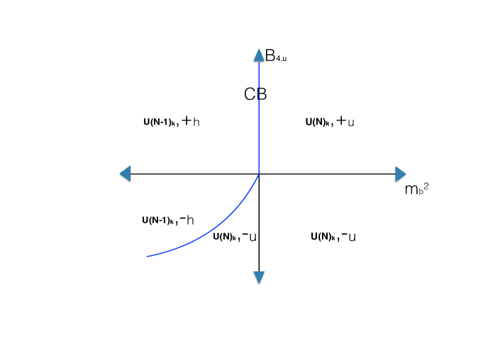
Figure 7: The phase diagram for $\displaystyle\phi_{1}<x_{6}<\phi_{2}$. For $\displaystyle B_{4,u}>0$ we have a second order phase transition at $\displaystyle m_{b}^{2}=0$ between $\displaystyle+_{u}$ and $\displaystyle+_{h}$ phases. For $\displaystyle B_{4,u}<0$, the blue line is a first order phase transition between the region in which the solution $\displaystyle-_{u}$ is the dominant phase and the region in which the $\displaystyle-_{h}$ solution dominates. Note that the first order phase transition is at $\displaystyle m_{b}^{2}>0$ for $\displaystyle x_{6}>(\phi_{1}+\phi_{2})/2$, but it is at $\displaystyle m_{b}^{2}<0$ otherwise. Our schematic phase diagram has been sketched for the latter case.

For $\displaystyle x_{6}>\phi_{2}$, $\displaystyle A_{h}$ remains negative as it was for $\displaystyle\phi_{1}<x_{6}<\phi_{2}$. It follows that the space of Higgsed solutions in this parameter regime is the same as for the case $\displaystyle\phi_{1}<x_{6}<\phi_{2}$ that we have just analyzed above. However $\displaystyle A_{u}$, which was positive in the earlier parametric regime, turns negative when $\displaystyle x_{6}>\phi_{2}$. It follows that the space of unHiggsed solutions changes in the manner we now describe.

For $\displaystyle B_{4,u}>0$, the $\displaystyle-_{u}$ solution exists for $\displaystyle m_{b}^{2}<-B_{4,u}^{2}/A_{u}$ while the $\displaystyle+_{u}$ solution exists in the range $\displaystyle 0<m_{b}^{2}<-B_{4,u}^{2}/A_{u}$. These two solutions merge smoothly at $\displaystyle m_{b}^{2}=-B_{4,u}^{2}/A_{u}$. For $\displaystyle m_{b}^{2}>-B_{4,u}^{2}/A_{u}$ there is no solution, unHiggsed or Higgsed, to the gap equations. Below this value there are always two solutions ($\displaystyle-_{u}$ and either $\displaystyle+_{u}$ or $\displaystyle+_{h}$ depending on whether $\displaystyle m_{b}^{2}$ is positive or negative). It turns out that the dominant solutions are the $\displaystyle+_{u}$ and $\displaystyle+_{h}$ solutions, so that the theory has a second order phase transition between these two solutions at $\displaystyle m_{b}^{2}=0$. The long distance behaviour of the phase transition point is again governed by the CB theory.

For $\displaystyle B_{4,u}<0$, the only unHiggsed solution is $\displaystyle+_{u}$, and this solution exists only when $\displaystyle m_{b}^{2}<0$. The Higgsed solutions are the same as above, so now we have no solutions when $\displaystyle m_{b}^{2}>-B_{4,h}^{2}/A_{h}$. Below this value we have the $\displaystyle-_{h}$ solution and either the $\displaystyle+_{u}$ or the $\displaystyle+_{h}$ solution, depending on whether $\displaystyle m_{b}^{2}$ is negative or positive (with a smooth transition between the latter when $\displaystyle m_{b}^{2}=0$). In this case it turns out that the $\displaystyle-_{h}$ solution dominates, so our theory is always in the Higgsed phase for negative $\displaystyle B_{4,u}$ and there are no phase transitions as $\displaystyle m_{b}^{2}\to 0$.

Again we find that nothing special happens as $\displaystyle b_{4}\to 0$ (with no solutions for $\displaystyle m_{b}^{2}>0$, and with the $\displaystyle-_{h}$ solution smoothly going into the $\displaystyle+_{h}$ solution for $\displaystyle m_{b}^{2}<0$). The full phase structure for this range of values of $\displaystyle x_{6}$ is drawn in figure 8.

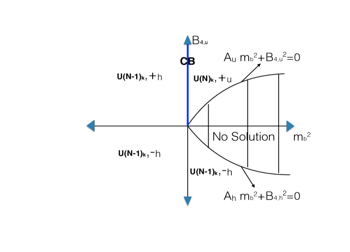
Figure 8: The phase diagram for $\displaystyle x_{6}>\phi_{2}$. For $\displaystyle B_{4,u}>0$ we have a second order phase transition at $\displaystyle m_{b}^{2}=0$ between $\displaystyle+_{u}$ and $\displaystyle+_{h}$ phases, while for $\displaystyle B_{4,u}<0$ the $\displaystyle-_{h}$ solution dominates whenever it exists. There are no solutions for large enough values of $\displaystyle m_{b}^{2}$.

Next, let us consider what happens when we increase $\displaystyle x_{6}$ to $\displaystyle\phi_{2}$, such that $\displaystyle A_{u}$ goes to zero and then becomes negative, while nothing special happens to the Higgsed solutions. Figures 7 and 8 suggest that in this limit nothing dramatic happens except in the lower right quadrant, and this is indeed the case. As $\displaystyle x_{6}\to\phi_{2}$, the $\displaystyle-_{u}$ solution has $\displaystyle|c_{B}|=-2B_{4,u}/A_{u}$, so it exists in the full region $\displaystyle B_{4,u}<0$ and its $\displaystyle|c_{B}|$ goes to infinity, and then for larger $\displaystyle x_{6}$ its $\displaystyle|c_{B}|$ becomes negative so that this solution no longer exists, leaving no solutions for $\displaystyle B_{4,u}<0$ and $\displaystyle m_{b}^{2}>-B_{4,h}^{2}/A_{h}$. As we pass $\displaystyle x_{6}=\phi_{2}$, the $\displaystyle-_{u}$ solution starts existing (as a sub-dominant solution) on the other side $\displaystyle B_{4,u}>0$, gradually coming down from $\displaystyle|c_{B}|=\infty$. On the other hand, the $\displaystyle+_{u}$ solution in this limit has $\displaystyle|c_{B}|=m_{b}^{2}/4B_{4,u}$, so it exists whenever this ratio is positive, and smoothly goes through $\displaystyle x_{6}=\phi_{2}$.

For $\displaystyle x_{6}<\phi_{1}$ the picture is essentially the same, just exchanging the unHiggsed and Higgsed phases, and the sign of $\displaystyle m_{b}^{2}$ – see figure 9 and the Appendix for more details.

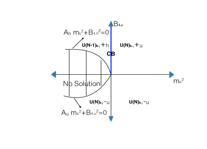
Figure 9: The phase diagram for $\displaystyle x_{6}<\phi_{1}$. For $\displaystyle B_{4,u}>0$ we have a second order phase transition at $\displaystyle m_{b}^{2}=0$ between $\displaystyle+_{u}$ and $\displaystyle+_{h}$ phases, while for $\displaystyle B_{4,u}<0$ the $\displaystyle-_{u}$ solution dominates whenever it exists. There are no solutions for small enough values of $\displaystyle m_{b}^{2}$.

4.3 A curious limit

Our discussion above implies (as we checked also in section 3.11 for finite temperatures) that for $\displaystyle B_{4,u}>0$ and $\displaystyle m_{b}^{2}=0$ the RB theory flows to the CB theory (for any value of $\displaystyle x_{6}$). Somewhat surprisingly, there is also another limit where this seems to be the case. Consider the limit

$$b_{4}=0~{},~{}x_{6}\rightarrow\infty,~{}m_{b}^{2}\rightarrow-\infty,$$ (202)

keeping the pole mass $\displaystyle c_{B}$ and $\displaystyle m_{B}^{cri}$ fixed, where

$$(m_{B}^{cri})^{2}\equiv-\frac{4m_{b}^{2}}{3x_{6}\lambda_{B}^{2}}.$$ (203)

In this limit we have two solutions to the RB theory’s finite temperature (and zero temperature) gap equations (above we called these solutions at zero temperature by different names when $\displaystyle B_{4,u}>0$ and when $\displaystyle B_{4,u}<0$, but they go smoothly through $\displaystyle B_{4,u}=0$). The first solution is to the gap equation (173) in the unHiggsed phase, and it is given by $\displaystyle{\tilde{S}}=\frac{|m_{B}^{cri}|}{2}$ ; note that this is the same as the gap equation of the CB theory in its unHiggsed phase (equation (73) with $\displaystyle{\rm sgn}(X_{B})=-{\rm sgn}(\lambda_{B})$). At the same values of the RB theory’s microscopic parameters, the equations for the Higgsed phase (172) reduce to

$$|c_{B}|=|\lambda_{B}|{\cal S}+\frac{|m_{B}^{cri}\lambda_{B}|}{2},$$ (204)

which agrees with the gap equation of the CB theory in its Higgsed phase (equation (73) with $\displaystyle{\rm sgn}(X_{B})={\rm sgn}(\lambda_{B})$).

The observations of the last paragraph suggest that there is a close connection between the scaling limit (202) and the critical boson theory; naively it seems that we flow to the latter theory at low energies. However, the relationship between the deformed RB theory and the CB theory is a curious one. To see this let us focus on the zero temperature limit.

In a deformed critical boson theory we are either in the Higgsed or unHiggsed phase depending on the value of the microscopic parameter $\displaystyle m_{B}^{cri}$; positive values of this parameter put us in the unHiggsed phase while negative values of this parameter put us in the Higgsed phase. This is clear, for instance, from figure 8.

In the scaling limit (202) of the RB theory, on the other hand, we found above that at the same value of the microscopic parameters there are two different phases, which both lie on the negative $\displaystyle m_{b}^{2}$ axis in figure 8. Recall that there are two solutions of the gap equation in all allowed regions of this figure; in figure 8 we drew only the thermodynamically dominant phase, while in fact for every value of $\displaystyle m_{b}^{2}$ and $\displaystyle b_{4}$ there is also another, thermodynamically sub-dominant phase; the two phases are analyzed in appendix F and depicted in figures 22(a) and 22(b). These two phases do not have the same free energy (the free energy of the Higgs phase is negative and dominates) and so at any finite $\displaystyle x_{6}$ the unHiggsed phase is unstable and decays. However, in the limit (202) the decay amplitude between these phases vanishes, so the deformed RB theory has two different effective superselection sectors (the Higgsed and unHiggsed saddle points of the RB theory, which are superselection sectors because tunneling switches off at large $\displaystyle x_{6}$). We can then identify these by the relations described above with the Higgsed and unHiggsed deformations of the CB theory, depending on our choice of the sign of $\displaystyle m_{B}^{cri}$ in (203). It seems that in the limit (202), the CB theory controls not just the region near the positive $\displaystyle B_{4,u}$ axis in figure 8, but also the region near the negative $\displaystyle m_{b}^{2}$ axis (note that in the $\displaystyle x_{6}\to\infty$ limit there are no solutions to the gap equation with finite $\displaystyle B_{4,u}$ and $\displaystyle m_{b}^{2}>0$).

It is clear that the relationship we found between the scaling limit (202) of the RB theory and the CB theory, for finite values of $\displaystyle m_{B}^{cri}$, cannot hold when $\displaystyle m_{B}^{cri}=0$. For one thing the conformal RB theory, which sits at the origin of figure 8, has a deformation (along the $\displaystyle m_{b}^{2}$ axis to the right) for which it has no solution to the gap equations. There is no analogue of this phenomenon in the CB theory. Also, the RB theory has a dimension 1 scalar operator at all finite values of $\displaystyle x_{6}$, while that is not the case for the CB theory. So the precise statement is that as $\displaystyle x_{6}$ becomes large at infinite $\displaystyle N$, the CB theory controls also flows along the negative $\displaystyle m_{b}^{2}$ axis, but not the point at the origin.

For finite $\displaystyle N$, as we have seen above, $\displaystyle x_{6}$ is not really a marginal parameter; RG flows dynamically drive large values of $\displaystyle x_{6}$ to infinity. So we can speculate that perhaps when we go to finite values of $\displaystyle N$, the relation between these theories can be extended also to the origin of the parameter space, when we start in the UV with $\displaystyle x_{6}\gg 0$. The naive expectations we described above for the behaviour of the RB theory may be significantly modified at $\displaystyle x_{6}\sim N_{B}^{\frac{1}{3}}$ (when the $\displaystyle\beta$ function of $\displaystyle x_{6}$ ceases to be small), and then the true end point of the RG flow along positive $\displaystyle x_{6}$ may genuinely be the CB theory. It is also possible that this is not the case. We leave further discussion of this issue to future work.

4.4 Interplay between the phase diagram and the RG fixed points

In section 4.2 we have worked out the phase diagram of the RB theory at infinite $\displaystyle N_{B}$; we discovered that the phase diagram changes qualitatively depending on where $\displaystyle x_{6}$ lies in relation to the distinguished values $\displaystyle\phi_{1}$ and $\displaystyle\phi_{2}$ defined in (200).

In section 3 we saw that $\displaystyle 1/N_{B}$ corrections cause $\displaystyle x_{6}$ to run. The running is governed by a $\displaystyle\beta$ function with three fixed points. In other words we can treat $\displaystyle x_{6}$ as a free parameter only in the strict large $\displaystyle N_{B}$ limit. At any finite $\displaystyle N_{B}$, no matter how large, we have true fixed points of the renormalization group only at these 3 particular values of $\displaystyle x_{6}$. The phase diagrams that we have evaluated in section 4.2 (which are approximately correct even at large but finite $\displaystyle N_{B}$, at any given value of $\displaystyle x_{6}$) are of most interest at the fixed point values of $\displaystyle x_{6}$. Thus it is of interest to understand where the three fixed point values of $\displaystyle x_{6}$ lie in relation to $\displaystyle\phi_{1}$ and $\displaystyle\phi_{2}$.

While $\displaystyle\phi_{1}$ and $\displaystyle\phi_{2}$ are known analytically at all $\displaystyle\lambda_{B}$ (see (200)), we do not have closed form expressions for the fixed point values of $\displaystyle x_{6}$ at arbitrary $\displaystyle\lambda_{B}$. However the corresponding expressions are available at small $\displaystyle|\lambda_{B}|$ (see (150)) and at small $\displaystyle 1-|\lambda_{B}|$ (see (158)). For these special cases we have sketched the relative positions of $\displaystyle\phi_{1}$, $\displaystyle\phi_{2}$ (blue stars) and of the three fixed points of the renormalization group (black dots) in Figure 10. We see from Figure 10 that in both of these cases the middle fixed point (the attractive fixed point about which the $\displaystyle x_{6}$ deformation is irrelevant, which has a total of two relevant deformations) lies in between $\displaystyle\phi_{1}$ and $\displaystyle\phi_{2}$. It is natural to conjecture that this continues to be the case at all values of $\displaystyle\lambda_{B}$, and thus that the phase structure of this attractive fixed point for large finite $\displaystyle N_{B}$ is given by figure 7.

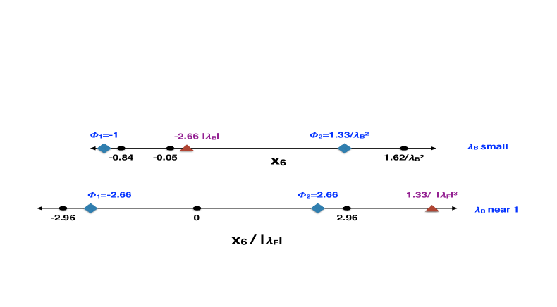
Figure 10: A sketch of the $\displaystyle x_{6}$ axis at small $\displaystyle|\lambda_{B}|$ and at small $\displaystyle 1-|\lambda_{B}|$. In each case we have plotted the three fixed points of the renormalization group as black dots, $\displaystyle\phi_{1}$ and $\displaystyle\phi_{2}$ as blue diamonds, and the end point of SUSY RG flows (discussed in the next section) as a red triangle. In the case of small $\displaystyle|\lambda_{B}|$ the fixed points of the RG flow are listed in (150), $\displaystyle\phi_{1}=-1$, $\displaystyle\phi_{2}\approx{4}/{(3|\lambda_{B}|^{2})}$, and the end point of the SUSY RG flow occurs at $\displaystyle-{8|\lambda_{B}|}/{3}$. At small $\displaystyle 1-|\lambda_{B}|$ the fixed points of the RG flow are listed in (158), $\displaystyle\phi_{1}$ and $\displaystyle\phi_{2}$ are $\displaystyle\approx\pm{8|\lambda_{F}|}/{3}$, and the end point of the SUSY RG flow occurs at $\displaystyle{4}/{(3|\lambda_{F}|^{2})}$.

Similarly, the rightmost fixed point is to the right of $\displaystyle\phi_{2}$ in both limits; there seems no reason to expect this to change at any value of $\displaystyle\lambda_{B}$. However the leftmost fixed point lies between $\displaystyle\phi_{1}$ and $\displaystyle\phi_{2}$ when $\displaystyle|\lambda_{B}|$ is small, but lies to the left of $\displaystyle\phi_{1}$ when $\displaystyle|\lambda_{B}|$ is near unity. It is likely that this fixed point will lie between $\displaystyle\phi_{1}$ and $\displaystyle\phi_{2}$ for all $\displaystyle|\lambda_{B}|$ less than some critical value that lies between zero and unity, but that it will lie to the left of $\displaystyle\phi_{1}$ for all $\displaystyle|\lambda_{B}|$ larger than this critical value.

4.5 Flows from Yang-Mills-Chern-Simons theories to Chern-Simons-matter theories

In this subsection we make some general remarks about the phase diagram one may expect for the RB theory from a particular point of view. The discussion in this subsection is very general, makes no reference to particular computations, and should apply even at finite $\displaystyle N_{B}$. At the end of this subsection we discuss the relationship between the general remarks of this subsection and the explicit phase diagrams presented earlier in this section.

As we mentioned in section 1.2, one way to analyze the existence of the fixed points (2)-(5) is to start at high energies with Yang-Mills-Chern-Simons (YM-CS) theories, with some gauge coupling $\displaystyle g_{YM}$ and level $\displaystyle\kappa$. At energies much larger than $\displaystyle g_{YM}^{2}N$ and $\displaystyle g_{YM}^{2}\kappa$ these theories are weakly coupled, so they provide good starting points for RG flows. In this section we analyze this flow in detail, and relate the resulting phase structure (which is reliable at energies above $\displaystyle g_{YM}^{2}$) to our analysis above of the phase structure of the fixed points (these arise here at energies well below $\displaystyle g_{YM}^{2}$). To be explicit we discuss here the $\displaystyle U(N)_{\kappa}$ theory, but the same general statements apply for $\displaystyle SU(N)_{\kappa}$ theories and for $\displaystyle U(N)$ theories with different levels for the $\displaystyle SU(N)$ and $\displaystyle U(1)$ factors; for finite $\displaystyle N$ and $\displaystyle\kappa$ the precise behaviour may be different for these other cases.

In order to analyze the theories we are interested in, it is useful to start from scalar fundamental fields coupled to the YM-CS theory. In this case we can add at high energies a scalar potential

$$V(\phi)=g_{2}|\phi|^{2}+g_{4}(|\phi|^{2})^{2}+g_{6}(|\phi^{2}|)^{3}.$$ (205)

For $\displaystyle g_{6}\neq 0$ the theory remains interacting also at high energies and it is not clear if it is well-defined, but if we choose $\displaystyle g_{6}=0$ then these theories are well-defined, for any value of $\displaystyle g_{2}$ and $\displaystyle g_{4}$ (generally $\displaystyle g_{6}$ is generated along the RG flow). Moreover, if we choose the values of $\displaystyle g_{2}$ and $\displaystyle g_{4}$ such that the scalar field becomes massive at a high scale (above $\displaystyle g_{YM}^{2}N$ and $\displaystyle g_{YM}^{2}\kappa$), then at that scale we can trust the analysis of the scalar using the potential (205), and below this scale we have a pure YM-CS theory which is believed to flow to a pure CS theory (for these values the Yang-Mills interactions are always small; the scalar self-interactions may be large, but they are not expected to change the qualitative form of (205)). Note that all these statements do not depend on taking any large $\displaystyle N$ or large $\displaystyle\kappa$ limits.

Let us begin with the case $\displaystyle g_{4}>0$ (and large in units of $\displaystyle g_{YM}^{2}N$ or $\displaystyle g_{YM}^{2}\kappa$; this is what we will mean by large throughout this subsection). If $\displaystyle g_{2}>0$ is also large, then $\displaystyle\phi$ is massive and has no expectation value, so that the low energy theory is a pure $\displaystyle U(N)_{\kappa}$ CS theory. On the other hand, if $\displaystyle g_{2}<0$ is large (in its absolute value), $\displaystyle\phi$ gets a large expectation value, such that at low energies we have a pure $\displaystyle U(N-1)_{\kappa}$ CS theory. As we change $\displaystyle g_{2}$ from large and negative to large and positive there has to be a phase transition. This may be a second (or higher) order phase transition as suggested by the classical potential (205), or a first order phase transition; since quantum corrections are important when $\displaystyle\phi$ is light and near the origin, this is difficult to analyze. Whenever we have a second order phase transition it is described by the CB theory, while for values of $\displaystyle N$ and $\displaystyle\kappa$ for which there is a first order transition it is not clear if the CB theory exists.

Next, consider the case of $\displaystyle g_{4}\ll 0$. The behaviour at large $\displaystyle\phi$ now depends on $\displaystyle g_{6}$, but since it vanishes (at the cutoff scale) it seems that there would be a runaway behaviour in this regime (the classical potential should be reliable at very large $\displaystyle\phi$ since quantum corrections are small there). If $\displaystyle g_{2}\gg 0$ we now have a massive meta-stable vacuum at the origin, in which the low-energy theory is given by the $\displaystyle U(N)_{\kappa}$ CS theory. For very large $\displaystyle g_{2}$ the life-time of this vacuum goes to infinity, so its existence is reliable. If $\displaystyle g_{2}\ll 0$ there is no meta-stable vacuum, and $\displaystyle\phi$ runs away to some large finite or infinite value. So again there is some phase transition as a function of $\displaystyle g_{2}$, and in this case it is clearly of first order (whenever stable vacua exist at large $\displaystyle\phi$).

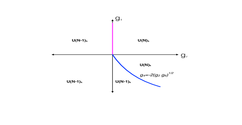
Figure 11: The phase structure of YM-CS theories as a function of the parameters of the scalar potential (205). This structure is reliable far away from the two axes, when both $\displaystyle|g_{2}|$ and $\displaystyle|g_{4}|$ are large; the regions marked by $\displaystyle U(N-1)_{\kappa}$ may instead involve runaway behaviour with no stable vacuum.

See figure 11 for the phase structure, assuming that there is a range of parameters where we flow to the CB theory; this is reliable when both $\displaystyle|g_{2}|$ and $\displaystyle|g_{4}|$ are large.

For all values of $\displaystyle g_{4}$ we thus have a transition as a function of $\displaystyle g_{2}$, between a vacuum at the origin and a situation where $\displaystyle\phi$ has an expectation value (or runs away to large $\displaystyle\phi$). Suppose that for $\displaystyle g_{4}\gg 0$ we have a second order phase transition and thus a CB theory. As we decrease $\displaystyle g_{4}$, at some point this line of second order phase transitions should end and become a line of first order phase transitions. Classically the end is at $\displaystyle g_{4}=0$ where we get an RB theory with $\displaystyle g_{6}=0$; in the quantum theory, with the gauge interactions and the running $\displaystyle g_{6}$, it is difficult to say where the line ends, but it ends somewhere. One option is that this end is a CB fixed point, but in this case it is difficult to see how a small deformation of this theory could lead to a theory with two stable vacua or with a runaway (as we have near the line of first order phase transitions); recall that the CB theory has a single stable vacuum for either sign of its deformation parameter. Thus, a more likely option seems to be that the end is an RB theory; since this theory has parameters corresponding to $\displaystyle g_{2}$ and $\displaystyle g_{4}$, it naturally leads to the correct phase diagram around it. This argument naively implies that whenever the CB theory exists as an IR limit of the corresponding YM-CS theory, the RB theory should exist as well. Note that in particular this is the case in the ungauged scalar theory, where the role of the RB theory is simply played by free massless scalars.

In the large $\displaystyle N$ limit we can try to relate the analysis here to our discussion of the running coupling. The coupling $\displaystyle g_{6}$ runs (at least below the scale $\displaystyle g_{YM}^{2}\kappa$), but for large $\displaystyle N$ it runs slowly (when we take $\displaystyle g_{6}=\lambda_{6}/N^{2}$ for fixed $\displaystyle\lambda_{6}$) since its beta function goes as $\displaystyle 1/N$, so one can approximate the RG flow to the end-point of the CB line, described in the previous paragraph, as leading to an RB-like theory with some value of $\displaystyle g_{6}$, and then $\displaystyle g_{6}$ continuing to slowly flow. Note that in this context we cannot choose the value of $\displaystyle g_{6}$, since there is a specific value that follows from the high-energy theory with $\displaystyle g_{6}=0$ that we specified. If $\displaystyle g_{6}$ flows to a fixed point then we get precisely the picture of the previous paragraph; in particular this picture requires that there is an IR-stable fixed point for $\displaystyle g_{6}$. However, from the point of view of the flow as a function of $\displaystyle g_{6}$ it is possible also to have $\displaystyle g_{6}$ flow to $\displaystyle(+\infty)$ or $\displaystyle(-\infty)$, and then we cannot use the Yang-Mills-Chern-Simons theories to define the quasi-bosonic fixed points. Note that at leading order in $\displaystyle 1/N$ our discussion of the beta function implies that large enough positive values of $\displaystyle\lambda_{6}$ will always flow to $\displaystyle(+\infty)$, and negative to $\displaystyle(-\infty)$, but for finite large $\displaystyle N$ this analysis is only valid when $\displaystyle\lambda_{6}$ does not scale with $\displaystyle N$, so it is possible that even large values of $\displaystyle|\lambda_{6}|$ may end up at a fixed point.

In section 4.2 we analyzed the large $\displaystyle N$ phase structure of the quasi-bosonic theories at large $\displaystyle N$ and zero temperature. This analysis is valid in an opposite regime from the one described above – namely when the deformation parameters $\displaystyle g_{2}$ and $\displaystyle g_{4}$ are much smaller than $\displaystyle g_{YM}^{2}N$ and $\displaystyle g_{YM}^{2}\kappa$ (which are taken to infinity in this paper). At infinite $\displaystyle N$, $\displaystyle g_{6}$ (or equivalently the parameter $\displaystyle x_{6}$ of the low-energy theory (93)) is exactly marginal and we can compute the phase structure of (205) as a function of this parameter. When it is small and positive we find the same phase structure as in our computation of section 4.2 (see figure 7), consistent with having the Yang-Mills-Chern-Simons theory flow to the RB fixed point at large $\displaystyle N$. In particular the RB theory flows after a mass deformation of the appropriate sign to the CB theory. For large $\displaystyle|x_{6}|$ we found in section 4.2 that the phase structure changes. There is still a CB line as described above, but for the other sign of the mass deformation there seems to be no stable vacuum (this agrees with the semi-classical expectation from (205) when $\displaystyle x_{6}<0$, but we find this behaviour also for positive $\displaystyle x_{6}$). Of course, when the coupling is not small there is no reason for the semi-classical analysis above to be valid. In the upcoming paper new an exact Landau Ginzburg description of the phase structure is presented which is consistent with our large $\displaystyle N$ results.

Note that the issues we discuss in this section are generally similar to the ones arising in the flow from the SUSY theory that we described in section 1.2; in both cases we have a well-defined UV starting point, but it is not clear what happens near the putative RB point. In the SUSY flow for large $\displaystyle N$ we could compute at which value of $\displaystyle x_{6}$ we end up, so that in some cases we know that we end up at a stable fixed point, while in this section it is not clear how to analyze this. It seems likely that the phase structure near the putative RB point is the same in both cases, but we do not know how to prove this. We can also discuss a similar UV completion for the CF theories (5), that should include a kinetic term for the scalar field $\displaystyle\zeta$ in addition to the Yang-Mills term; we expect this to be analogous to our discussion here.

5 The $\displaystyle{\cal N}=2$ superconformal Chern-Simons-matter theory

In this section we study RG flows emanating from the $\displaystyle{\cal N}=2$ superconformal Chern-Simons-matter theory with a single fundamental chiral multiplet. In components, the matter content of this theory is a single fundamental complex boson $\displaystyle\phi$ plus a single fundamental complex fermion $\displaystyle\psi$, each minimally coupled to a Chern-Simons gauge field. As in the previous sections the gauge group can be either $\displaystyle SU(N)_{\kappa^{{\cal N}=2}}$ or $\displaystyle U(N)_{\kappa^{{\cal N}=2},\kappa^{{\cal N}=2}_{2}}$ (see Appendix D for notation). This will affect the precise form of the duality in the SUSY theory (and in the resulting non-SUSY theories), but it will not matter for our leading-order (in $\displaystyle 1/N$) computations.

We will use the results of Jain:2013gza to study the RG flows seeded by relevant deformations from this fixed point. In particular we begin with a pair of superconformal field theories that are dual to each other by the generalizations of the Giveon-Kutasov duality Benini:2011mf , and construct fine-tuned large $\displaystyle N$ RG flows that begin at these superconformal theories and end on the RB/CF theories at a particular value of $\displaystyle x_{6}$. The flows from the superconformal fixed point to the RB/CF theories are seeded by operators that are relevant even in the strict large $\displaystyle N$ limit and so are ‘fast flows’ in the sense that they take place over ratios of scales of order unity. Once these flows have settled down into the RB/CF manifolds, the much slower flow of $\displaystyle x_{6}$ – governed by the $\displaystyle\beta$ functions computed in detail in section 3 – ensues over RG flow ‘times’ of order $\displaystyle N$, and our analysis in this section does not add any information about the end-point of these flows. However, the flows in this section are well-defined even for finite $\displaystyle N$, at least if $\displaystyle N$ is large enough, so one can conjecture that they may end (for appropriate fine-tunings) at RB/CF fixed points even for small values of $\displaystyle N$.

5.1 Lagrangian

After integrating out all auxiliary fields, and working with the dimensional reduction scheme (which is convenient for actual computations), the Lagrangian of a general $\displaystyle U(N)_{\kappa^{{\cal N}=2},\kappa^{{\cal N}=2}_{2}}$ theory with the same field content as the SUSY theory takes the form

$$\displaystyle S \displaystyle=\int d^{3}x\biggl{[}i\varepsilon^{\mu\nu\rho}{\kappa\over 4\pi}\mathrm{Tr}(A_{\mu}\partial_{\nu}A_{\rho}-{2i\over 3}A_{\mu}A_{\nu}A_{\rho})+i\varepsilon^{\mu\nu\rho}{\kappa_{2}\over 4\pi}B_{\mu}\partial_{\nu}B_{\rho}$$

$$\displaystyle+D_{\mu}\bar{\phi}D^{\mu}\phi+\bar{\psi}\gamma^{\mu}D_{\mu}\psi+m_{B}^{2}\bar{\phi}\phi+m_{F}\bar{\psi}\psi+{4\pi b_{4}\over\kappa}(\bar{\phi}\phi)^{2}+\frac{4\pi^{2}x_{6}}{\kappa^{2}}(\bar{\phi}\phi)^{3}$$

$$\displaystyle+\frac{4\pi x_{4}}{\kappa}(\bar{\psi}\psi)(\bar{\phi}\phi)+\frac{2\pi y_{4}^{\prime}}{\kappa}(\bar{\psi}\phi)(\bar{\phi}\psi)+\frac{2\pi y_{4}^{\prime\prime}}{\kappa}\left((\bar{\psi}\phi)(\bar{\psi}\phi)+(\bar{\phi}\psi)(\bar{\phi}\psi)\right)\biggl{]},$$ (206)

with

$$\kappa=\kappa^{{\cal N}=2},~{}~{}~{}\kappa_{2}=\kappa^{{\cal N}=2}_{2}.$$ (207)

In the $\displaystyle{\cal N}=2$ superconformal theory the coupling constants are given by

$$m_{F}=m_{B}=b_{4}=y_{4}^{\prime\prime}=0,~{}~{}~{}x_{4}=x_{6}=y_{4}^{\prime}=1.$$ (208)

Here $\displaystyle A_{\mu}$ is an $\displaystyle SU(N)$ gauge field, $\displaystyle B_{\mu}$ is a $\displaystyle U(1)$ gauge field and the covariant derivatives are defined as in (12). The Lagrangian for the $\displaystyle SU(N)_{\kappa^{{\cal N}=2}}$ theory is the same as (206), but with $\displaystyle B_{\mu}$ set to zero. We review the SUSY dualities between these theories in appendix E.

5.2 Marginal and relevant deformations

The $\displaystyle{\cal N}=2$ supersymmetric theory defined in the previous subsection enjoys invariance under $\displaystyle{\cal N}=2$ superconformal symmetry. In particular it is a fixed point under the renormalization group. In this section we will enumerate the relevant and marginal deformations about this fixed point.

In the large $\displaystyle N$ limit this fixed point has 3 relevant deformations ($\displaystyle m_{B}^{2}$, $\displaystyle m_{F}$ and $\displaystyle b_{4}$ in (206)) together with four exactly marginal deformations ($\displaystyle x_{6}$, $\displaystyle x_{4}$, $\displaystyle y_{4}^{\prime}$ and $\displaystyle y_{4}^{\prime\prime}$). At large but finite $\displaystyle N$ these operators get anomalous dimensions. Actually these anomalous dimensions are not all independent; some are related to others by supersymmetry as we now explain.

Consider the superconformal operator $\displaystyle O=\left(\mathrm{Tr}({\bar{\phi}}\phi)\right)^{2}$. The supersymmetric descendents $\displaystyle Q_{\alpha}{\bar{Q}}^{\alpha}O$ and $\displaystyle\left(Q_{\alpha}Q^{\alpha}+{\bar{Q}}_{\alpha}{\bar{Q}}^{\alpha}\right)O$ are linear combinations of the four operators parameterized by $\displaystyle x_{6}$, $\displaystyle x_{4}$, $\displaystyle y_{4}^{\prime}$ and $\displaystyle y_{4}^{\prime\prime}$. It follows that the anomalous dimensions of the four large $\displaystyle N$ marginal operators are determined by those of $\displaystyle O$ plus two additional independent anomalous dimensions. Explicit calculation at weak coupling (to order $\displaystyle\lambda^{2}$) reveals that all these three independent anomalous dimensions are positive (see Table 1 for a listing of the leading weak coupling results quoted from Avdeev:1992jt ).

Eigen Vector	Eigen Value
$\displaystyle{\delta m_{B}}$	$\displaystyle 0$
$\displaystyle-\frac{{\delta m_{F}}}{4\pi\lambda}\frac{N^{2}}{N-1}+\frac{4\pi\lambda}{N}{\delta b_{4}}$	$\displaystyle 0$
$\displaystyle\frac{4\pi}{k}{\delta b_{4}}$	$\displaystyle\frac{16\pi^{2}\lambda^{2}(N-1)\left(8N^{2}+7N-16\right)}{N^{4}}$
$\displaystyle-\frac{4\pi^{2}{\delta x_{6}}\lambda^{2}}{N^{2}}$	$\displaystyle\frac{48\pi^{2}\lambda^{2}(N-1)(N(8N+17)-26)}{N^{4}}$
$\displaystyle\frac{8\pi\lambda}{N}{\delta y}_{4}^{\prime\prime}$	$\displaystyle\frac{16\pi^{2}\lambda^{2}(N-1)(N(8N+7)-16)}{N^{4}}$
$\displaystyle\frac{N(2{\delta x}_{4}+{\delta y}_{4}^{\prime})}{2(N-1)}-\frac{4\pi^{2}{\delta x}_{6}\lambda^{2}}{N^{2}}$	$\displaystyle\frac{16\pi^{2}\lambda^{2}(N-1)(N(8N+7)-16)}{N^{4}}$
$\displaystyle\frac{N(4N(8N(N+1)-47)+127)(2{\delta x}_{4}-\delta y_{4}^{\prime})}{6(N-1)(2N-1)(4N-3)}-\frac{4\pi^{2}{\delta x}_{6}\lambda^{2}}{N^{2}}$	$\displaystyle\frac{16\pi^{2}\lambda^{2}(N+1)(N(8N+9)-20)}{3N^{4}}$

Table 1: The leading weak coupling anomalous dimensions about the $\displaystyle{\cal N}=2$ $\displaystyle SU(N)$ superconformal point. The first column lists the flow eigenvectors in the notation of (207), while the second column lists the eigenvalues (corrections to the classical dimensions of the corresponding operators). The first two lines assert that the mass operators, which preserve SUSY, receive no anomalous dimensions. The third line of the table lists the positive anomalous dimension of the superconformal primary $\displaystyle(\mathrm{Tr}({\bar{\phi}}\phi))^{2}$. The fifth and sixth lines assert that the descendants of this operator share the same anomalous dimensions. The fourth line lists the positive anomalous dimension of the primary operator $\displaystyle(\mathrm{Tr}({\bar{\phi}}\phi))^{3}$. The seventh line of the table lists the positive anomalous dimension of a superconformal primary which is built out of linear combinations of products of descendants of $\displaystyle\mathrm{Tr}({\bar{\phi}}\phi)$.

At weak gauge coupling it follows that all the large $\displaystyle N$ marginal operators are in fact irrelevant, and the $\displaystyle{\cal N}=2$ fixed point has three relevant deformations. Although it will not be very important for the rest of this paper, there is no reason to believe that this qualitative pattern does not persist at all values of the level and the rank.

It follows that at any finite $\displaystyle N$ the Lagrangian (206) really defines a quantum field theory only upon setting

$$y_{4}^{\prime\prime}=0,~{}~{}~{}x_{4}=x_{6}=y_{4}^{\prime}=1.$$ (209)

As the anomalous dimensions that reveal this fact are all of order $\displaystyle\frac{1}{N}$, however, calculations performed in the strict large $\displaystyle N$ limit are well-defined for all values of these four parameters. Below we will present results for the free energy of these theories in the strict large $\displaystyle N$ limit for arbitrary values of these parameters simply because we can, and then insert (209) into our final results.

5.3 The partition function along general large $\displaystyle N$ RG flows

At leading order in the large $\displaystyle N$ limit the operators parameterized by $\displaystyle x_{6}$, $\displaystyle x_{4}$, $\displaystyle y_{4}^{\prime}$ and $\displaystyle y_{4}^{\prime\prime}$ are all exactly marginal, and there exists a 6 parameter set of RG flows (corresponding to a seven parameter set of quantum field theories) emanating out of the $\displaystyle{\cal N}=2$ supersymmetric fixed point. This seven parameter set of theories was listed in (206). Note that the generic theory in this 7 parameter space is not supersymmetric. Several quantities in these theories can be computed in the large $\displaystyle N$ limit as we now review.

The simplest physical quantities one can compute from this Lagrangian are the pole masses of the boson and the fermion. One can demonstrate (see Jain:2013gza for details) that the zero temperature bosonic/fermionic propagators have poles at $\displaystyle p^{2}+c_{B,0}^{2}=0$ and $\displaystyle p^{2}+c_{F,0}^{2}=0$, respectively, where $\displaystyle c_{B,0}$ and $\displaystyle c_{F,0}$ obey the following equations:

$$c^{2}_{B,0}=\lambda^{2}(1+3x_{6})\frac{c^{2}_{B,0}}{4}-2\lambda b_{4}|c_{B,0}|+x_{4}\frac{\lambda(-\lambda+2~{}\text{sgn}(\rm{X_{0}}))}{(\lambda-\text{sgn}(\rm{X_{0}}))^{2}}(-m_{F}+x_{4}\lambda|c_{B,0}|)^{2}+m_{B}^{2},$$ (210)

$$c^{2}_{F,0}=\left({m_{F}-x_{4}|c_{B,0}|\lambda\over-\lambda+\text{sgn}(\rm{X_{0}})}\right)^{2},$$ (211)

where

$$X_{0}=\lambda\left(c_{F,0}-x_{4}c_{B,0}\right)+m_{F}.$$ (212)

Following the discussion of subsection 2.3 one can also compute the finite temperature sphere partition function of these theories. The relevant gap equations for the theory of this subsection turn out to be

$$c_{F}^{2}=(2\lambda({\cal C}-x_{4}{\cal S})+{\hat{m}}_{F})^{2},$$ (213)

$$c_{B}^{2}=\lambda^{2}(1+3x_{6}){\cal S}^{2}-4\lambda{\hat{b}}_{4}{\cal S}+4x_{4}(\lambda^{2}{\cal C}^{2}-2x_{4}\lambda^{2}{\cal S}{\cal C}+{\hat{m}}_{F}\lambda{\cal C})+{\hat{m}_{B}}^{2}$$ (214)

(see (78) for definitions of $\displaystyle{\cal C}$ and $\displaystyle{\cal S}$). These gap equations were demonstrated in Jain:2013gza to enjoy a self duality under the transformations

$$\begin{split}&N^{\prime}=|\kappa|-N,~{}~{}~{}\kappa^{\prime}=-\kappa,~{}~{}~{}x_{4}^{\prime}={1\over x_{4}},\quad m_{F}^{\prime}=-\frac{m_{F}}{x_{4}},\quad\lambda^{\prime}=\lambda-\text{sgn}(\lambda),\\ &x_{6}^{\prime}=1+\frac{1-x_{6}}{x_{4}^{3}},\quad b_{4}^{\prime}=-\frac{1}{x_{4}^{2}}(b_{4}+\frac{3}{4}\frac{1-x_{6}}{x_{4}}m_{F}),\\ &m_{B}^{\prime 2}=-\frac{1}{x_{4}}m_{B}^{2}+\frac{3}{4}\frac{1-x_{6}}{x_{4}^{3}}m_{F}^{2}+\frac{2}{x_{4}^{2}}b_{4}m_{F}.\end{split}$$ (215)

More concretely the gap equations transform back to themselves, provided we also make the identifications

$$\begin{split}&c_{B}^{\prime}=c_{F},~{}~{}~{}c_{F}^{\prime}=c_{B},\\ &\lambda^{\prime}{\cal S}^{\prime}=-\frac{\text{sgn}(\lambda)}{2}|c_{F}|+\lambda{\cal C},\\ &\lambda^{\prime}{\cal C}^{\prime}=-\frac{\text{sgn}(\lambda)}{2}|c_{B}|+\lambda{\cal S}\end{split}$$ (216)

(see subsection 2.3 for more discussion).

The first line in (LABEL:dualofq) reflects the fact that bosons and fermions are interchanged under the conjectured self duality of these deformed $\displaystyle{\cal N}=2$ theories. Note that the $\displaystyle{\cal N}=2$ theories (208) map to themselves by (215), which agrees with the known $\displaystyle{\cal N}=2$ dualities Benini:2011mf . In particular, the restriction to the renormalizable manifold (209) is preserved by the duality map (215).

5.4 Flows to purely bosonic or fermionic theories

The authors of Jain:2013gza demonstrated that under a one parameter fine-tuning, the gap equations (213) and (214) of the typical RG flow away from the $\displaystyle{\cal N}=2$ fixed point reduce in the low-energy limit to the gap equation for the critical boson and regular fermion theories, respectively, providing strong evidence for such RG flows at large $\displaystyle N$. RG flows from the theories (206) are parameterized by the ratios of $\displaystyle m_{B}$, $\displaystyle m_{F}$ and $\displaystyle b_{4}$ (which all have the same dimension in the large $\displaystyle N$ limit), so we have two parameters to play around with, which we will denote by $\displaystyle a_{0}=m_{B}^{2}/m_{F}^{2}$ and $\displaystyle g_{0}=b_{4}/m_{F}$. The one parameter fine-tuning was needed because each of these IR theories has a single relevant deformation.

In the rest of this section we will demonstrate that the gap equations (213) and (214) of the generic RG flow away from the $\displaystyle{\cal N}=2$ fixed point also reduce at low energies to the gap equation for the regular boson and critical fermion theories, respectively, after a two parameter fine-tuning (namely, choosing specific values for $\displaystyle a_{0}$ and $\displaystyle g_{0}$). We need a two parameter fine-tuning because these IR theories each have two relevant deformations. As discussed in great detail above, the IR theories in the strict large $\displaystyle N$ limit each also possess a marginal operator parameterized by $\displaystyle x_{6}$. The two parameter fine tuned large $\displaystyle N$ flows end up in the IR theories at values of $\displaystyle x_{6}$ that depend on the 4 (large $\displaystyle N$) marginal parameters of the starting UV theory. If, on the other hand, we start our flow in the UV at the SUSY theory (209) (as we appear to be forced to do, if we want flows that extend all the way to the UV and make sense at any finite $\displaystyle N$ no matter how large) all these 4 ‘marginal’ parameters are fixed. We have no extra parameters to tune, so that we end up in the IR at a specific value $\displaystyle x_{6}$ that depends on $\displaystyle\lambda$ (see below).

Let us repeat the bose-fermi gap equations (213) and (214) for convenience:

$$\begin{split}c_{F}^{2}&=(2\lambda({\cal C}-x_{4}{\cal S})+{\hat{m}}_{F})^{2},\\ c_{B}^{2}&=\lambda^{2}(1+3x_{6}){\cal S}^{2}-4\lambda{\hat{b}}_{4}{\cal S}+4x_{4}(\lambda^{2}{\cal C}^{2}-2x_{4}\lambda^{2}{\cal S}{\cal C}+{\hat{m}}_{F}\lambda{\cal C})+{\hat{m}}_{B}^{2}.\\ \end{split}$$ (217)

We will be interested in flows in which one of $\displaystyle c_{B}$ or $\displaystyle c_{F}$ is held fixed, with the other one taken to infinity. In taking the large $\displaystyle c_{B}$ or $\displaystyle c_{F}$ limit it is useful to note that

$$\begin{split}&{\cal C}\rightarrow\frac{|c_{F}|}{2}~{}~{}~{}~{}~{}~{}~{}~{}~{}{\rm{in~{}the~{}limit}}~{}~{}c_{F}\rightarrow\infty,\\ &{\cal S}\rightarrow\frac{|c_{B}|}{2}~{}~{}~{}~{}~{}~{}~{}~{}~{}{\rm{in~{}the~{}limit}}~{}~{}c_{B}\rightarrow\infty.\end{split}$$ (218)

5.5 Fermionic scaling limits

In order to analyze the end-points of the RG flows from the theories (206) we want to take some or all of $\displaystyle m_{F}$, $\displaystyle m_{B}$ and $\displaystyle b_{4}$ to infinity with fixed ratios. We begin by analyzing fermionic scaling limits, in which we end up in the IR in a fermionic theory, namely with a finite value of $\displaystyle c_{F}$ and an infinite value of $\displaystyle c_{B}$.

Let us begin by considering a flow ending up at a fine-tuned fermionic fixed point with $\displaystyle c_{F,0}=0$. Using (211), obtaining $\displaystyle c_{F,0}=0$ is the same as obtaining $\displaystyle|c_{B,0}|=m_{F}/x_{4}\lambda$, and plugging this into (210) gives us a relation between the parameters $\displaystyle m_{B}^{2}$, $\displaystyle b_{4}$ and $\displaystyle m_{F}$. Equivalently, we can use (211) to determine $\displaystyle|c_{B,0}|$ in terms of $\displaystyle|c_{F,0}|$ (and other parameters). Plugging this expression into (210), we obtain a quadratic equation for $\displaystyle|c_{F,0}|$ which can be cast into the schematic form

$$\left(|c_{F,0}|-f_{1}(a_{0},g_{0},x_{4},x_{6},\lambda)\right)\left(|c_{F,0}|-f_{2}(a_{0},g_{0},x_{4},x_{6},\lambda)\right)=0,$$ (219)

where we have defined

$$a_{0}\equiv\frac{m_{B}^{2}}{m_{F}^{2}},~{}~{}~{}g_{0}\equiv\frac{b_{4}}{m_{F}}.$$ (220)

It is easy to check that $\displaystyle|c_{F,0}|=0$ is a solution to (219) (i.e. that either $\displaystyle f_{1}$ or $\displaystyle f_{2}$ vanish) if and only if

$$a_{0}=\frac{\lambda^{2}\left(8g_{0}x_{4}-3x_{6}-1\right)+4}{4\lambda^{2}x_{4}^{2}}.$$ (221)

This is the same fine-tuning that was performed in Jain:2013gza . Specializing to the case (209) in which the theory is supersymmetric in the UV, (221) simplifies to

$$a_{0}=2g_{0}-1+{1\over\lambda^{2}}.$$ (222)

It is easy to check that for generic values of $\displaystyle g_{0}$, $\displaystyle c_{B,0}$ diverges as $\displaystyle m_{F}\to\infty$. So for such generic values we expect to land in the RF theory, and we expect (and will soon check) that a small deviation in $\displaystyle a_{0}$ away from (221) (of order $\displaystyle 1/m_{F}$) will generate a finite mass deformation of the RF theory. However, there may be a special fine-tuned value of $\displaystyle g_{0}$ for which we end up in the CF theory. If this turns out to be the case, then near this value small deviations of $\displaystyle a_{0}$ and $\displaystyle g_{0}$ (of order $\displaystyle 1/m_{F}$) will correspond to turning on the two relevant deformations of the CF theory ($\displaystyle\sigma$ and $\displaystyle\sigma^{2}$ in the language of the previous sections). In particular, one combination of these deformations - the one that turns on $\displaystyle\sigma^{2}$ but not $\displaystyle\sigma$ - should leave $\displaystyle c_{F,0}=0$. This can only happen if (219) has a double zero at the special tuned values of $\displaystyle a_{0}$ and $\displaystyle g_{0}$, i.e. if $\displaystyle f_{1}$ and $\displaystyle f_{2}$ in (219) both vanish. In that case the deformation that preserves (221) could leave, say, $\displaystyle f_{1}=0$ while changing $\displaystyle f_{2}$ (this is the $\displaystyle\sigma^{2}$ deformation). It is straightforward to check that (219) has a double zero when

$$g_{0}=-{1\over{x_{4}\lambda^{2}}}+{{1+3x_{6}}\over{4x_{4}}},\qquad\qquad a_{0}={g_{0}\over x_{4}}.$$ (223)

In the case that the theory is SUSY in the UV (209) the values are

$$a_{0}=g_{0}=1-{1\over\lambda^{2}}.$$ (224)

Thus, for these specially tuned values it is plausible that the RG flow ends up in the IR at the CF theory rather than the RF theory.

We will now test this guess by demonstrating that in the limits above (and small deviations thereof), the thermodynamic expressions reduce to those of the (deformed) RF and CF theories. In order to show this, let us parameterize the small deviations from (221) by taking

$$m_{F}\rightarrow\infty,\qquad m_{B}^{2}=a_{1}m_{F}^{2}+a_{2}m_{F}+a_{3},\qquad b_{4}=g_{1}m_{F}+g_{2},$$ (225)

where

$$\begin{split}&a_{1}=\frac{\lambda^{2}\left(8g_{1}x_{4}-3x_{6}-1\right)+4}{4\lambda^{2}x_{4}^{2}},~{}~{}a_{2}=\frac{2g_{2}}{x_{4}}-\frac{m_{F}^{\rm{reg}}\left(\lambda^{2}\left(4g_{1}x_{4}-3x_{6}-1\right)+4\right)}{2\lambda^{2}x_{4}^{2}},\\ &a_{3}=(m_{F}^{\rm{reg}})^{2}\left(x_{4}\frac{\lambda\left(\lambda-2\text{sgn}(m_{F}^{\rm{reg}})\right)}{\left(\text{sgn}(m_{F}^{\rm{reg}})-\lambda\right)^{2}}+\frac{\frac{4}{\lambda^{2}}-3x_{6}-1}{4x_{4}^{2}}\right)-\frac{2g_{2}m_{F}^{\rm{reg}}}{x_{4}}.\end{split}$$ (226)

This reproduces (221) for infinite $\displaystyle m_{F}$ (where $\displaystyle a_{0}\to a_{1}$, $\displaystyle g_{0}\to g_{1}$), but now we include also small deviations of $\displaystyle a_{0}$ and $\displaystyle g_{0}$. As we take $\displaystyle m_{F}\to\infty$ we keep fixed (in addition to $\displaystyle x_{4}$, $\displaystyle x_{6}$ and $\displaystyle g_{1}$) also the two parameters of dimension mass, $\displaystyle g_{2}$ and $\displaystyle m_{F}^{\rm{reg}}$.

Let us analyze the thermodynamics and the gap equations in the limit (225). We will soon see that, in the limit under consideration, $\displaystyle c_{B}\to\infty$. Consequently, we can use the second of (LABEL:scaa) to simplify the gap equations (217). We find that the second of (217) is obeyed at order $\displaystyle{\cal O}(m_{F}^{2})$ provided we choose

$$c_{B}=\frac{{\hat{m}}_{F}}{x_{4}\lambda}+\delta c_{B},$$ (227)

where $\displaystyle\delta c_{B}$ is of order $\displaystyle m_{F}^{0}$ (recall that $\displaystyle{\hat{m}}_{F}$ is $\displaystyle m_{F}$ measured in units of the temperature). Plugging (227) into the second of (217), we find that the term in this equation of order $\displaystyle{\cal O}(m_{F})$ is proportional to

$$\left(g_{1}+\frac{3}{4}x_{4}^{2}x_{6}^{F}\right)\left(\delta c_{B}+\frac{{\hat{m}}_{F}^{\rm{reg}}}{x_{4}\lambda}\right),$$ (228)

where

$$x_{6}^{F}\equiv\frac{4}{3x_{4}^{3}\lambda_{F}^{2}}-\frac{1+3x_{6}}{3x_{4}^{3}}.$$ (229)

Now we see that we have two options; either the expression in the first parenthesis in (228) or the second one should vanish. Above we identified the first case as the CF flow (223), so let us start with the second case,

$$g_{1}\neq-\frac{3}{4}x_{4}^{2}x_{6}^{F},$$ (230)

which we expect to lead to the RF theory; we must then have

$$\delta c_{B}=-\frac{{\hat{m}}_{F}^{\rm{reg}}}{x_{4}\lambda},$$ (231)

or

$$c_{B}=\frac{{\hat{m}}_{F}-{\hat{m}}_{F}^{\rm{reg}}}{x_{4}\lambda}+{\cal O}\left(\frac{1}{{\hat{m}}_{F}}\right).$$ (232)

Plugging (232) into the second of (217) we find that the terms involving $\displaystyle{\hat{m}_{F}}$ in that equation all cancel (indeed the scalings (225), (226) were chosen to ensure precisely this cancellation) and the first of (217) turns into

$${\cal C}=\frac{\text{sgn}(\lambda)|c_{F}|-{\hat{m}}_{F}^{\rm{reg}}}{2\lambda}+{\cal O}\left(\frac{1}{{\hat{m}}_{F}}\right).$$ (233)

(233) is the same as (77), establishing that in the scaling limit (225) with (230), the thermodynamics of the deformed theory (206) reduces to (a finite deformation of) the regular fermion theory. Recall that the pole mass of the regular fermion theory, $\displaystyle c_{F,0}$, is related to $\displaystyle m_{F}^{\rm{reg}}$ by the equation

$$|c_{F,0}|=\frac{m_{F}^{\rm{reg}}}{{\text{sgn}(m_{F}^{\rm{reg}})}-\lambda}.$$ (234)

5.5.1 Critical fermionic limit

Next, let us check what happens when $\displaystyle g_{1}$ is tuned to take the special value

$$g_{1}=-\frac{3}{4}x_{4}^{2}x_{6}^{F},$$ (235)

which we expect to lead to (a finite deformation of) the CF theory.

In studying this particular case we find it convenient to reexpress the parameter $\displaystyle g_{2}$ of the previous subsubsection in terms of another parameter $\displaystyle y_{4}$ defined by

$$g_{2}=-x_{4}^{2}y_{4}$$ (236)

(note that $\displaystyle g_{2}$ and $\displaystyle y_{4}$ both have the dimension of mass). We also find it useful to reexpress the parameter $\displaystyle m_{F}^{\rm{reg}}$ of the previous subsubsection in terms of yet another parameter $\displaystyle y_{2}$ (also with the dimension of a mass), defined by

$$a_{3}=-x_{4}y_{2}^{2}.\quad$$ (237)

With these choices and definitions we have

$$a_{1}=-\frac{3}{4}x_{4}x_{6}^{F},\quad a_{2}=-2x_{4}y_{4}.\quad$$ (238)

As above we define the order unity quantity $\displaystyle\delta c_{B}$ by (227), and determine it by requiring that the second of (217) be obeyed at subleading order. As above, the leading term in (227) ensures that the second of (217) is obeyed to order $\displaystyle m_{F}^{2}$. It follows from (228) that, at our special value of $\displaystyle g_{1}$, this equation is also automatically obeyed at order $\displaystyle m_{F}$ for any choice of $\displaystyle\delta c_{B}$. In order to determine $\displaystyle\delta c_{B}$ we then require that the equation be obeyed at order unity. Let

$$c_{B}=\frac{1}{x_{4}\lambda}{\hat{m}}_{F}-\frac{{\hat{\sigma}}_{F}}{x_{4}\lambda},$$ (239)

where the order unity quantity $\displaystyle{\hat{\sigma}}_{F}$ is a rescaled version of $\displaystyle\delta c_{B}$. It may be shown that the second of (217) is obeyed at order unity provided

$$0=\frac{3}{4}\hat{\sigma}_{F}^{2}x_{6}^{F}-4\hat{\sigma}_{F}\lambda{\cal C}+2\hat{\sigma}_{F}\hat{y}_{4}-4\lambda^{2}{\cal C}^{2}+\hat{y}_{2}^{2}.$$ (240)

Using (239) and (240), the fermionic gap equation then reduces to

$$c_{F}^{2}=\left(2\lambda{\cal C}+{\hat{\sigma}}_{F}\right)^{2}.$$ (241)

(241) and (240) match perfectly with (176) and (178), respectively, if we identify $\displaystyle{\hat{y}}_{4}$ and $\displaystyle{\hat{y}}_{2}$ with the two relevant deformations of the CF theory, and we identify $\displaystyle x_{6}^{F}$ of that theory with $\displaystyle x_{6}^{F}$ defined by (229). It follows that the flow defined in this section yields the critical fermion theory with these parameters.

In particular, deforming away from the CF point along the line (221) corresponds to turning on the $\displaystyle y_{4}$ deformation, that for one sign induces a flow towards the RF theory. However, as discussed in section 4, for the other sign we expect that this flow will lead to a situation where for every $\displaystyle y_{2}$ we have a gapped theory (perhaps with a first order phase transition) or no vacuum at all, rather than a second order phase transition, so we do not expect any fixed points for these values of $\displaystyle y_{4}$ (see the phase diagrams sketched in Figs 7, Figure 8 and Figure 9 ). The coefficient of the $\displaystyle\zeta^{2}$ term that we add to the CF Euclidean action in (3.11) is proportional to $\displaystyle(-y_{4}\lambda)$, and we expect that when this is large and positive we will reach the RF point. This means that $\displaystyle g_{2}\text{sgn}(\lambda)$ should be above some upper bound, which means that our change in $\displaystyle g_{0}\simeq g_{1}+g_{2}/m_{F}$ should have the same sign as that of $\displaystyle\lambda m_{F}$. Translating back to our original variables, we conclude that the RG flow should only reach the RF theory when

$$\text{sgn}(\lambda m_{F})g_{0}>\text{sgn}(\lambda m_{F})\left[-{1\over{x_{4}\lambda^{2}}}+{{1+3x_{6}}\over{4x_{4}}}\right]$$ (242)

and $\displaystyle a_{0}$ is given by (221), namely along a half-infinite-line in the $\displaystyle(a_{0},g_{0})$ plane. In the SUSY case this becomes

$$\text{sgn}(\lambda m_{F})g_{0}>\text{sgn}(\lambda m_{F})\left[1-{1\over\lambda^{2}}\right],\qquad\qquad a_{0}=2g_{0}-1+{1\over\lambda^{2}}.$$ (243)

Let us now focus on the special case $\displaystyle y_{2}=y_{4}=0$. In this limit (238) defines an RG flow that ends up precisely on the line of critical fermion theories. Restricting attention to RG flows that originate on the renormalizable (SUSY at high energies) manifold (209), it follows from (229) that we land on this line of theories at

$$x^{F}_{6}=\frac{4}{3}\left(\frac{1}{\lambda^{2}}-1\right).$$ (244)

At small values of $\displaystyle\lambda$, the value of $\displaystyle x_{6}^{F}$ listed in (244) lies far outside the domain of attraction (169) of the stable fixed point of the RG flow, so in this case, at large $\displaystyle N$, the RG flow of this section does not reach this stable fixed point. For other values of $\displaystyle x_{4}$ and $\displaystyle x_{6}$ we end up at other values of $\displaystyle x_{6}^{F}$ in the IR, including values within this domain of attraction, but this observation appears to be of limited significance for reasons discussed above.

5.6 Bosonic scaling Limits

Let us now repeat the analysis of the previous section for bosonic scaling limits, in which we want to end up at a finite value of $\displaystyle c_{B}$ but an infinite value of $\displaystyle c_{F}$. We begin by considering a flow that should land precisely on a bosonic critical point with $\displaystyle c_{B,0}=0$. Using (210) this gives a simple relation between $\displaystyle m_{B}$ and $\displaystyle m_{F}$, such that

$$a_{0}=x_{4}-\frac{x_{4}}{\left(\text{sgn}(m_{F})-\lambda\right)^{2}},$$ (245)

while $\displaystyle g_{0}$ can take any value. This is the same as the bosonic flow discussed in Jain:2013gza .

As in the discussion above, we expect generic values of $\displaystyle g_{0}$ to end up in the CB theory, but there may be a special value where we end up in the RB theory, and for this value we expect $\displaystyle c_{B,0}=0$ to be a double root of (210). Requiring that the linear term in this equation vanish gives us the extra condition

$$g_{0}=x_{4}^{2}\left(1-\frac{1}{(\text{sgn}(m_{F})-\lambda)^{2}}\right),$$ (246)

with $\displaystyle a_{0}$ still given by (245); note that again we find $\displaystyle g_{0}=x_{4}a_{0}$, just like in the CF flow.

Let us again check these expectations by matching the thermodynamics of the limit theories to that of the CB and RB theories. We now choose to parameterize the small deviations from the flows mentioned above by (using the same notations as in (225))

$$\begin{split}&a_{1}=x_{4}-\frac{x_{4}}{\left(\text{sgn}(m_{F})-\lambda\right)^{2}},~{}~{}a_{2}=2m_{B}^{\rm{cri}}\lambda\left(x_{4}^{2}\left(\frac{1}{\left(\text{sgn}(m_{F})-\lambda\right)^{2}}-1\right)+g_{1}\right),\\ &a_{3}=\frac{1}{4}\left(m_{B}^{\rm{cri}}\right)^{2}\left(\lambda^{2}x_{4}^{3}\left(4-\frac{4}{\left(\text{sgn}(m_{F})-\lambda\right)^{2}}\right)-(3x_{6}+1)\lambda^{2}+4\right)+2m_{B}^{\rm{cri}}g_{2}\lambda.\end{split}$$ (247)

We then take the limit $\displaystyle m_{F}\to\infty$ with the dimensionless parameters $\displaystyle x_{4}$ and $\displaystyle x_{6}$ together with $\displaystyle g_{1}$, $\displaystyle g_{2}$ and $\displaystyle m_{B}^{\rm{cri}}$ held fixed. In this limit, as we will see below, $\displaystyle c_{F}\to\infty$. Consequently we can use the first of (LABEL:scaa) to simplify the gap equations (217). To leading order in $\displaystyle m_{F}$ we find

$$c_{F}=\frac{{\hat{m}}_{F}}{\text{sgn}(m_{F})-\lambda}+{\cal O}(1).$$ (248)

When we plug (248) into the first of (217) we find that all terms at leading order (order $\displaystyle m_{F}^{2}$) in this equation cancel, while the equation is not satisfied at first subleading order (order $\displaystyle m_{F}$). We find it convenient to parameterize the $\displaystyle{\cal O}(1)$ correction to the solution (248) by the order unity quantity $\displaystyle\delta c_{F}$ defined by

$$c_{F}=\frac{{\hat{m}}_{F}-\delta c_{F}x_{4}\lambda}{\text{sgn}(m_{F})-\lambda}.$$ (249)

When we plug (249) into the first of (217), collect all terms of order $\displaystyle m_{F}$, and equate their sum to zero, we find the equation

$${\cal S}=\frac{\delta c_{F}}{2}.$$ (250)

Now using (247) and (250), the second equation of (217) is automatically solved at leading order (order $\displaystyle m_{F}^{2}$) but is nontrivial at first subleading order (order $\displaystyle m_{F}$). At this order the equation takes the form

$$\left(g_{1}-x_{4}^{2}\left(1-\frac{1}{(\text{sgn}(m_{F})-\lambda)^{2}}\right)\right)\left(2{\cal S}-{\hat{m}}_{B}^{\rm{cri}}\right)=0.$$ (251)

Let us begin by looking at the solutions to (251) with

$$g_{1}\neq x_{4}^{2}\left(1-\frac{1}{(\text{sgn}(m_{F})-\lambda)^{2}}\right),$$ (252)

which we expect to flow to the CB theory. In this case we find

$${\cal S}=\frac{{\hat{m}}_{B}^{\rm{cri}}}{2}+{\cal O}\left(\frac{1}{{\hat{m}}_{F}}\right),$$ (253)

which agrees with (76), establishing that the general theory reduces, in the scaling limit of the present subsubsection, to the critical boson theory with mass parameter $\displaystyle{\hat{m}}_{B}^{\rm{cri}}$.

5.6.1 Regular bosonic scaling limit

Let us now study the special case

$$g_{1}=x_{4}^{2}\left(1-\frac{1}{(\text{sgn}(m_{F})-\lambda)^{2}}\right),$$ (254)

which as discussed above we expect to flow to the RB theory. We find it convenient to rename the parameter $\displaystyle g_{2}$ (with the dimensions of mass) as

$$g_{2}=b_{4}.$$ (255)

We will also trade the fixed mass $\displaystyle m_{B}^{\rm{cri}}$ used in above for another fixed mass $\displaystyle{\tilde{m}}_{B}$ defined by

$$a_{3}={\tilde{m}}_{B}^{2}.$$ (256)

With these choices we have

$$\begin{split}a_{1}&=x_{4}\left(1-\frac{1}{(\text{sgn}(m_{F})-\lambda)^{2}}\right),\qquad a_{2}=0,,\\ \end{split}$$ (257)

Once again we insert the expansion (249) into the fermionic gap equation and find (250), so that

$$c_{F}=\frac{{\hat{m}}_{F}}{\text{sgn}(m_{F})-\lambda}-2{\mathcal{S}}\frac{x_{4}\lambda_{B}}{\text{sgn}(m_{F})-\lambda}.$$ (258)

As explained above, once we plug (258) into the bosonic gap equation ( the second of (217)) at the special value of $\displaystyle g_{1}$ (254), we find that this equation is automatically satisfied both at leading order (order $\displaystyle m_{F}^{2}$) and at first subleading order (order $\displaystyle m_{F}$). The equation is first nontrivial at order unity, and yields

$${c_{B}^{2}}=(4+3x_{6}^{B})\lambda^{2}{\cal S}^{2}-4\lambda\hat{b}_{4}{\cal S}+\hat{m}_{B}^{2},$$ (259)

with

$$x_{6}^{B}=(x_{6}-1)-\frac{4}{3}x_{4}^{3}\left(1-\frac{1}{(\text{sgn}(m_{F})-\lambda)^{2}}\right).$$ (260)

Note that (260) agrees perfectly with (173), if we identify the parameters of this subsection with those describing the RB theory, establishing that the scaling limit of the theory (206) considered in this subsubsection is simply the regular boson theory described in previous sections.

As in our discussion of the previous subsection, deformations away from the RB point by the parameter $\displaystyle b_{4}$ should change $\displaystyle g_{0}$ while preserving (245), and by looking at the RB action we expect a non-trivial CB fixed point to arise when $\displaystyle(b_{4}\lambda)$ is large and positive (this is justified by the analysis of section 4. Mapping this to the change in the sign of $\displaystyle g_{0}$ using (255), we expect a flow to the CB theory when

$$\text{sgn}(m_{F}\lambda)g_{0}>\text{sgn}(m_{F}\lambda)x_{4}^{2}\left(1-\frac{1}{(\text{sgn}(m_{F})-\lambda)^{2}}\right).$$ (261)

For other values of $\displaystyle g_{0}$ we do not expect to land at any critical point. As expected (naively) given (206), we find using $\displaystyle g_{0}=b_{4}/m_{F}$ that in the regime where $\displaystyle(b_{4}\lambda)$ of our deformation is large and positive we end up at a non-critical fixed point, while when it is large and negative we do not.

When our RG flows start on the renormalizable (SUSY) manifold (209), (260) simplifies to

$$x_{6}^{B}=-\frac{4}{3}\left(1-\frac{1}{(1-|\lambda|)^{2}}\right)=-\frac{8|\lambda|}{3}+{\cal O}(\lambda^{2}).$$ (262)

In particular, setting $\displaystyle b_{4}={\tilde{m}}_{B}^{2}=0$, we have a flow from the renormalizable sub-manifold of (206) to the point on the regular boson manifold of theories with $\displaystyle x_{6}^{B}$ listed in (262). Notice that this flow at small $\displaystyle\lambda$ lands well within the domain of attraction of the stable fixed point (153). It follows that the subsequent RG flow of the regular boson theory, which occurs over an RG flow time of order $\displaystyle N$, lands up in the stable fixed point of the finite $\displaystyle N$ regular boson theory at small $\displaystyle\lambda_{B}$. Once again, for infinite $\displaystyle N$ we can make other choices of $\displaystyle x_{4}$ and $\displaystyle x_{6}$ giving different values of $\displaystyle x_{6}^{B}$, but such flows are not UV-complete at finite values of $\displaystyle N$.

5.7 Duality of the scaling limits

We can use (215) to show that the duality of the boson+fermion theories (206) maps a flow labeled by $\displaystyle(a_{0},g_{0})$ at some coupling $\displaystyle\lambda$, to a flow labeled by

$$a_{0}^{\prime}=-x_{4}a_{0}+\frac{3(1-x_{6})}{x_{4}}+2g_{0},\qquad\qquad g_{0}^{\prime}=\frac{g_{0}}{x_{4}}+\frac{3(1-x_{6})}{4x_{4}^{2}}$$ (263)

in the theory with coupling $\displaystyle\lambda^{\prime}=\lambda-\text{sgn}(\lambda)$, with $\displaystyle x_{4}$ and $\displaystyle x_{6}$ of the two sides related as in (215). In particular, the deformation away from the SUSY theory labeled by $\displaystyle(a_{0},g_{0})$ at some coupling $\displaystyle\lambda$ maps in the dual theory to a deformation by $\displaystyle(2g_{0}-a_{0},g_{0})$.

As expected, this mapping takes the general fermionic scaling limit (221) to the general bosonic scaling limit (245). Moreover, it also maps the flow (223) to the CF point to the flow (246) to the RB point, and, moreover, it maps the second-order-phase-transition range (242) of the fermionic flow to the analogous range (261) in the bosonic flow. Thus, starting from the general duality of (206), and in particular the SUSY duality, and following our flows, leads to a duality between the RF and CB points as shown in Jain:2013gza , and also to a duality between the CF and RB points. At infinite $\displaystyle N$ our computation derives this, and we will discuss the finite $\displaystyle N$ situation in the next subsection.

Comparing in more detail the flows that end up slightly away from the RF/CB points, we find that in addition to relating $\displaystyle g_{1}^{\prime}$ and $\displaystyle g_{1}$ by (263), we should also take $\displaystyle g_{2}^{\prime}=-g_{2}/x_{4}^{2}$, and then we obtain $\displaystyle-\lambda_{B}m_{B}^{{\rm cri}}=m_{F}^{\rm reg}$ as expected from the RF/CB duality (71).

Similarly, if we follow the flows that go close to the CF/RB points, we find that the duality mapping of their parameters leading to a mapping taking

$$y_{4}=b_{4},~{}~{}y_{2}^{2}={\tilde{m}}_{B}^{2},$$ (264)

in perfect agreement with (184).

5.8 The end-points of RG flows

Starting from the SUSY theory, the RG flows (222) and (245) lead to ‘phases’ which are governed by the RF and CB theories, respectively. This point was noted in Jain:2013gza , where it was also noticed that the lines (222) and (245) cross each other. At this crossing point the authors of Jain:2013gza proposed (see section 3.3 of that paper) that the dynamics is that of a critical boson and a regular fermion interacting with each other. We believe that this conclusion is incorrect; the analysis of section 3.3 of Jain:2013gza ignored a subtlety that we now explain.

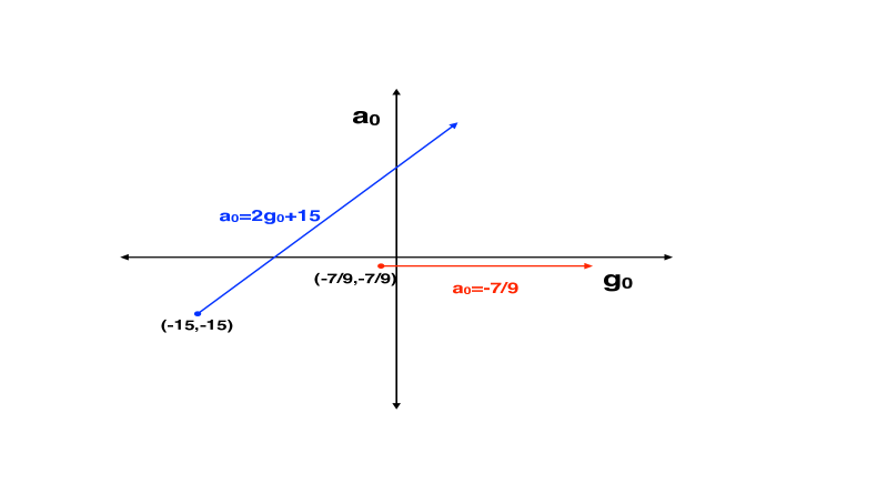
Figure 12: A sketch of the RG flows originating in the SUSY theory at $\displaystyle\lambda=1/4$ and with $\displaystyle m_{F}>0$. On a generic point along the blue ray (222) we flow to the RF theory; at the beginning of this ray, the point $\displaystyle(-15,-15)$, we flow to the CF theory. On a generic point on the horizontal red ray (245) we flow to the CB theory; at the beginning of this ray we flow to the RB theory. Note that the two rays nowhere intersect, so the SUSY theory never flows to the CB+RF theory.

As we have analyzed in great detail above, in certain ranges of parameters the CB theory (and so the RF theory and the supersymmetric theory) has multiple solutions to the gap equation. The RF fixed point is the dominant fixed point along the line (222) when the inequality (243) is obeyed (when the inequality is saturated we find the CF theory with $\displaystyle x_{6}^{F}$ given by (229)). Similarly the CB theory is the dominant solution to the gap equation along the curve (245) only when the inequality (261) is obeyed (when the inequality is saturated we find the RB theory with $\displaystyle x_{6}^{B}$ given by (260)). In other words we actually have RF and CB dynamics along rays (semi-infinite lines) rather than infinite lines in the $\displaystyle(g_{0},a_{0})$ plane. In Figure 12 we have sketched the half lines (222) subject to the inequality (243), and (245) subject to the inequality (261), in the special case $\displaystyle{\rm sgn}(m_{F})\lambda=\frac{1}{4}$. As is apparent from the figure, the two half lines do not, in fact, meet.

This conclusion holds at generic values of $\displaystyle\lambda$. It turns out that the intersection of the lines (221) and (245) happens at a value of $\displaystyle g_{0}$ that is exactly half of the sum of the critical $\displaystyle g_{0}$ (223) for the CF flow and the critical $\displaystyle g_{0}$ (246) for the RB flow. It follows that unless these two critical values are equal to each other, we are always above one of them and below the other, such that exactly one of the inequalities (242) and (261) is not satisfied. So we never end up at a RF+CB point. This does not mean that such a point, that was recently analyzed in Benini:2017aed ; Jensen:2017bjo , does not exist, but just that it does not arise as the end-point of an RG flow from our boson+fermion theories (206); it can perhaps arise from more general flows in which we have more independent fine-tunings of the deformations away from such a fixed point. There is a special choice of the parameters for which the two critical values of $\displaystyle g_{0}$ are equal to each other, so that we do have a flow that ends at a CF+RB point; this happens when

$${1\over 4}(3x_{6}+1)={1\over\lambda^{2}}+x_{4}^{3}\left[1-{1\over{(\text{sgn}(\lambda)-\lambda)^{2}}}\right].$$ (265)

In the supersymmetric case $\displaystyle x_{4}=x_{6}=1$ this happens for $\displaystyle\lambda=\pm{1\over 2}$.

At finite $\displaystyle N$ several things change. For large but finite values of $\displaystyle N$, one change is that the only UV-complete flow starts from the SUSY theory with $\displaystyle x_{4}=x_{6}=1$; but in practice we can also consider other values of $\displaystyle x_{4}$ and $\displaystyle x_{6}$, treating them as effective field theories that have some UV completion at higher energies (recall that the beta functions of $\displaystyle x_{4}$ and $\displaystyle x_{6}$ vanish at large $\displaystyle N$, so these effective actions can be valid over a large range of energies). Near the IR we should have a small shift in the position of the RF and CB lines, but they should still exist, and end at some point. The big difference is that now this point looks approximately like a CF/RB theory with some value of $\displaystyle x_{6}$, and this value now starts slowly running. This flow may approach a non-trivial CF/RB fixed point, or it make take $\displaystyle x_{6}$ to infinity. We expect to have some range of values of $\displaystyle\lambda$ for which we flow to a CF/RB point, assuming that it exists, while for other values we do not flow to this point (but it may still exist). For $\displaystyle x_{4}=x_{6}=1$ we drew in figure 10 the position of the end-point of the ‘fast flow’ at large $\displaystyle N$, which sometimes flows to a stable CF/RB point and sometimes does not.

At smaller values of $\displaystyle N$, the flow could change more dramatically. It is possible that one of the three relevant operators that we deform by could become irrelevant, and then we would only have a one-parameter set of flows, that can perhaps be fine-tuned to land at an RF/CB fixed point, but not at a CF/RB point. Conversely, it is also possible that more operators become relevant, but this would not change the number of required fine-tunings. We do not know for which range of values of $\displaystyle N$ and $\displaystyle k$ the RF/CB point exists; it is possible that for some values there is no second order phase transition at all. When this fixed point exists we do expect to have a flow from the SUSY theory to it as in large $\displaystyle N$, and then the flow line has to end as in the figure above. But as we discussed, it is not obvious that this end-point is a new fixed point, and it could also be a RF/CB point.

6 Discussion and future directions

The three main results of this paper are the computation of the large $\displaystyle N_{B}$ beta function for the parameter $\displaystyle x_{6}$ of quasi-bosonic theories, the elaboration of the zero temperature phase structure of these theories, and the study of flows from SUSY theories to quasi-bosonic theories. We begin this discussion section by considering each of these topics in turn.

Our final result for the beta function of RB theories, at leading nontrivial order in $\displaystyle\frac{1}{N_{B}}$, is presented in (94) and (97). Unfortunately this result is not completely explicit. We have demonstrated that the beta function is a cubic polynomial in $\displaystyle x_{6}$ and have computed two of the four coefficients of this polynomial at all orders in $\displaystyle\lambda_{B}$. However the remaining coefficients of this polynomial are known only in terms of three functions of $\displaystyle\lambda_{B}$ that characterize aspects of correlation functions of $\displaystyle{\tilde{J}}_{0}$ in the critical boson theory; the corresponding functions are only known explicitly at small $\displaystyle\lambda_{B}$ or small $\displaystyle\lambda_{F}$, but are not explicitly known at arbitrary $\displaystyle\lambda_{B}$. It would be very satisfying to complete the computation initiated in this paper by explicitly determining these three unknown functions.

One of the functions that we need in order to complete the evaluation of our $\displaystyle\beta$ function is the quantity $\displaystyle g_{(5,0)}$ defined in (58). This coefficient characterizes a particular kinematical limit of the 5-point function of scalar operators in the CB theory at leading order in the large $\displaystyle N_{B}$ limit. We suspect that the evaluation of this coefficient at all values of $\displaystyle\lambda_{B}$ may not prove too difficult a task (see Yacoby:2018yvy for recent progress). The remaining two coefficients that we need deal with $\displaystyle 1/N_{B}$ corrections to correlators. The first of these quantities is the anomalous dimension of $\displaystyle{\tilde{J}}_{0}$ at first order in the $\displaystyle 1/N_{B}$ expansion (see (16)). The second of these is the quantity $\displaystyle r_{B}$ that governs the splitting of the three point function of three $\displaystyle{\tilde{J}}_{0}$ operators into a contact piece and a power law piece (see (LABEL:thptdet)). As both of these quantities refer to subleading orders in the $\displaystyle 1/N_{B}$ expansion they may not be easy to compute by direct diagrammatic evaluation. Other approaches, such as the conformal bootstrap, may prove to be better for the evaluation of these quantities (see Turiaci:2018nua ; Aharony:2018npf for some recent progress on the bootstrap approach).

The deformed supersymmetric theory that we have studied in section 5 has a rich phase structure as a function of two dimensionless parameters (dimensionless ratios of the coefficients of the three relevant operators of the theory). While we have already analyzed several aspects of the phase structure of this theory in Section 5, it would be useful to complete this analysis in a completely systematic manner. The end point of such an analysis would be a detailed phase diagram of the theory along the lines of our analysis of the phase diagram of the RB theory section 4. In order to accomplish this we would need to generalize the free energy computation of Jain:2013gza to include Higgsed phases, along the lines of the recent computation Choudhury:2018iwf .

The CB and RF theories are believed to be dual to Vasiliev theories of gravity with a specific boundary condition for the scalar field on $\displaystyle AdS_{4}$, such that its classical dimension is $\displaystyle\Delta=2$. At finite values of $\displaystyle N$ the quantum gravitational theories can be defined using the three dimensional CFTs. Our discussion suggests that we can use the RB and CF theories to define quantum gravitational theories with other boundary conditions for the bulk scalar field, in which its classical dimension is $\displaystyle\Delta=1$. In the bulk the coupling $\displaystyle x_{6}^{B}$ (or $\displaystyle x_{6}^{F}$) in (4) (or (5)) is a “multi-trace” coupling that defines the precise boundary condition for the bulk scalar field, and our results imply that only specific values for this coupling really lead to consistent quantum theories on $\displaystyle AdS_{4}$. It would be nice to verify this directly by bulk computations; the bulk computation of beta functions for multi-trace couplings was discussed at the classical level in Witten:2001ua ; Grozdanov:2011aa ; Das:2013qea ; Aharony:2015afa , but in our case we expect the leading contribution to arise at one-loop order in the bulk.

There are many possible generalizations of our results :

• In this paper we only discuss theories with a single matter field in the fundamental representation. However, a similar picture is believed to hold also for larger numbers $\displaystyle N_{f}$ of matter fields, at least when these numbers are small enough compared to $\displaystyle N$ and $\displaystyle\kappa$ Seiberg:2016gmd ; Hsin:2016blu . For $\displaystyle N_{f}>1$ the flow diagrams are more complicated, since the RB and CF theories contain one additional relevant deformation (with a different contraction of the flavor indices), and two additional classically marginal deformations. We conjecture that there still exist fixed points leading to a duality between RB and CF theories, with one or both of the extra relevant deformations tuned to zero, but additional evidence is required to bring this conjecture to the same level as the $\displaystyle N_{f}=1$ conjecture that we discuss here. In particular one has to compute the beta functions for all three classically marginal operators.

• In this paper we discussed the phase structure of the regular boson theories at zero temperature, and found an intricate structure, where for some parameters there is no solution to the gap equations, suggesting a runaway behaviour. It would be interesting to generalize this analysis to finite temperature, and to see if this stabilizes the cases with no stable vacuum, and how the phase structure is deformed.

• It would be interesting to generalize the flow from theory S to the bosonic and fermionic theories to $\displaystyle SO(N)$ gauge groups, in order to provide more evidence for the $\displaystyle SO(N)$ dualities Aharony:2016jvv at finite $\displaystyle N$. This is more complicated than the $\displaystyle U(N)$ case because the supersymmetric theory has complex matter fields, while the simplest $\displaystyle SO(N)$ duality involves real matter fields.

• It would be interesting to study the duality between the RB and CF theories for small values of $\displaystyle N$, as in Seiberg:2016gmd ; Hsin:2016blu , to provide evidence for or against their validity for these values. Note that for the $\displaystyle SU(1)$ theories the RB theory is free (at low energies), as was the case for the RF theory in Seiberg:2016gmd ; Hsin:2016blu . It would, of course, be fascinating if the theories discussed in this paper continue to be well-defined (and to enjoy invariance under duality) at small finite values of $\displaystyle N$. It would be even more satisfying if these small $\displaystyle N$ theories made an appearance in experimentally relevant condensed matter systems (which allow for two fine-tunings of parameters).

We leave all these issues for future study.

Appendix A Constraints on the $\displaystyle{\tilde{J}}_{0}$ three point function from conformal invariance

As we have explained in the main text, the three point function of $\displaystyle{\tilde{J}}_{0}$ takes the form (23). In this subsection we will study the expression for $\displaystyle F(q_{1},q_{2},q_{3},\epsilon)$, and in particular find the leading dependence of this quantity on $\displaystyle\ln(\Lambda)$ at small

$$\epsilon\equiv\frac{\delta_{B}(\lambda_{B})}{\kappa_{B}},$$ (266)

which is the anomalous dimension of $\displaystyle{\tilde{J}}_{0}$ to first subleading order in $\displaystyle\frac{1}{N_{B}}$.

The explicit expression for $\displaystyle F(q_{1},q_{2},q_{3},\frac{\delta_{B}}{\kappa_{B}})$ is given by Bzowski:2013sza :

$$F(q_{1},q_{2},q_{3},\epsilon)={\cal N}\Lambda^{-3\epsilon}(q_{1}q_{2}q_{3})^{\frac{1}{2}+\epsilon}\int_{0}^{\infty}dx\sqrt{x}K_{\frac{1}{2}+\epsilon}(xq_{1})K_{\frac{1}{2}+\epsilon}(xq_{2})K_{\frac{1}{2}+\epsilon}(xq_{3}),$$ (267)

where $\displaystyle\Lambda$ is a UV cutoff, and $\displaystyle{\cal N}$ is a normalization constant of order unity that we will tune for later convenience. As mentioned above, $\displaystyle F(q_{1},q_{2},q_{3},\epsilon)$ is the Fourier transform of the expression

$$\frac{\Lambda^{-3\epsilon}}{(x_{1}-x_{2})^{2+\epsilon}(x_{2}-x_{3})^{2+\epsilon}(x_{3}-x_{1})^{2+\epsilon}}$$ (268)

up to a normalization that tends to a finite non-zero number in the limit $\displaystyle\epsilon\to 0$.

The integral in (267) is convergent for $\displaystyle\epsilon<0$, and is defined for arbitrary values of $\displaystyle\epsilon$ by analytic continuation from these values. As the integral diverges logarithmically at $\displaystyle\epsilon=0$ (the divergence comes the neighborhood of $\displaystyle x=0$), the expression for $\displaystyle F$ has a pole at $\displaystyle\epsilon=0$. Using the fact that $\displaystyle K_{\frac{1}{2}}(x)\propto\frac{e^{-x}}{\sqrt{x}}$ together with the small argument expansion of the Bessel function, it is easy to convince oneself that

$$F(q_{1},q_{2},q_{3},\epsilon)=\frac{1}{\epsilon}\left(\frac{\Lambda}{q_{1}+q_{2}+q_{3}}\right)^{-3\epsilon}\left(1+{\cal O}(\epsilon)\right).$$ (269)

Recall that $\displaystyle\epsilon={\cal O}(\frac{1}{N}).$ It follows that the function $\displaystyle\epsilon F$ admits the expansion

$$\epsilon~{}F=1-3\epsilon~{}\ln\left(\frac{\Lambda}{q_{1}+q_{2}+q_{3}}\right)+{\cal O}(\epsilon^{2}).$$ (270)

Appendix B The critical boson theory at $\displaystyle\lambda_{B}=0$

In this Appendix we compute two, three and four point functions of the operator $\displaystyle{\tilde{J}}_{0}=\sigma$ in the critical boson theory in the limit $\displaystyle\lambda_{B}\to 0$, at leading order in the large $\displaystyle N_{B}$ expansion. As a check on our results we compute the anomalous dimension of $\displaystyle\sigma$ to first order in the expansion in $\displaystyle\frac{1}{N_{B}}$, and recover the known result for this quantity.

In order to compute $\displaystyle\sigma$ correlators, we start with (11), and integrate out the (free) boson fields to obtain an effective action for $\displaystyle\sigma$. Tree graphs of this effectively classical action then generate correlators of $\displaystyle\sigma$ at leading order in $\displaystyle N_{B}$. Loops of the same effective action determine the anomalous dimension of $\displaystyle\sigma$.

B.1 $\displaystyle S_{eff}(\sigma)$ and $\displaystyle\sigma$ Green’s functions at leading order in $\displaystyle\frac{1}{N}$

In this subsection we study $\displaystyle S_{eff}(\sigma)$ and the Green’s functions of $\displaystyle\sigma$ at quadratic, cubic, quartic and pentic order. All through this appendix we work with the theory at $\displaystyle\lambda_{B}=0$. In this subsection we focus on the leading order in an expansion in $\displaystyle\frac{1}{N_{B}}$. In the next subsection we turn to a discussion of the first corrections in $\displaystyle\frac{1}{N_{B}}$.

At $\displaystyle\lambda_{B}=0$ the scalar field $\displaystyle\phi$ is easily integrated out of (11) so that

$$\begin{split}&\int D\phi e^{-\int\left(\partial{\bar{\phi}}\partial\phi+\sigma{\bar{\phi}}\phi\right)}=e^{-S_{eff}(\sigma)}\\ &S_{eff}(\sigma)=\sum_{n=2}^{\infty}\frac{1}{n!}\int dp_{n}{\tilde{S}}_{n}(-p_{i})\sigma(p_{1})\ldots\sigma(p_{n}),\end{split}$$ (271)

where $\displaystyle dp_{n}$ was defined in (101) (and includes a momentum delta function).

B.1.1 Quadratic and cubic order

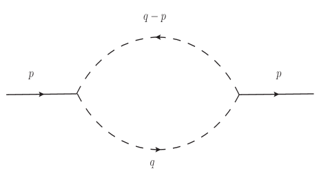
Figure 13: This diagram defines $\displaystyle{\tilde{S}}_{2}(p)$ in (272).

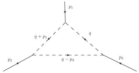
Figure 14: This diagram defines $\displaystyle{\tilde{S}}_{3}(p_{1},p_{2},p_{3})$ in (272).

The quadratic and cubic terms in this effective action are very easily computed. The relevant graph at quadratic order in presented in Figure 13; the relevant graph at cubic order is presented in Figure 14. Both graphs are easily evaluated and we find

$$\begin{split}&{\tilde{S}}_{2}(p)=-N_{B}\int\frac{d^{3}q}{(2\pi)^{3}}\frac{1}{q^{2}(p-q)^{2}}=-N_{B}\frac{1}{8|p|},\\ &{\tilde{S}}_{3}(p_{1},p_{2},p_{3})=2N_{B}\int\frac{d^{3}q}{(2\pi)^{3}}\frac{1}{q^{2}(p_{1}+q)^{2}(q-p_{3})^{2}}=\frac{N_{B}}{4}\frac{1}{|p_{1}||p_{2}||p_{3}|}.\end{split}$$ (272)

The two and three point Green’s functions for $\displaystyle\sigma$ follow immediately from these results. The two point function is simply the inverse of $\displaystyle{\tilde{S}}_{2}(p)$ and agrees with (20) at $\displaystyle\lambda=0$. The three point function is given by

$$\frac{{\tilde{S}}_{3}(p_{1},p_{2},p_{3})}{{\tilde{S}}_{2}(p_{1}){\tilde{S}}_{2}(p_{2}){\tilde{S}}_{2}(p_{3})}$$ (273)

and reduces to (28) upon setting $\displaystyle\lambda_{B}=0$.

B.1.2 The quartic term

The quartic term in the effective action is given by

$$\begin{split}&{\tilde{S}}_{4}(p_{1},p_{2},p_{3},p_{4})=-N_{B}\Bigg{(}W(p_{1},p_{2},p_{3},p_{4})+W(p_{1},p_{2},p_{4},p_{3})+W(p_{1},p_{4},p_{3},p_{2})\\ &\qquad\qquad\qquad\qquad\qquad+W(p_{1},p_{4},p_{2},p_{3})+W(p_{1},p_{3},p_{4},p_{2})+W(p_{1},p_{3},p_{2},p_{4})\Bigg{)},\\ \end{split}$$ (274)

where (see Figure 15)

$$W(p_{1},p_{2},p_{3},p_{4})\equiv\int\frac{d^{3}q}{(2\pi)^{3}}\frac{1}{q^{2}(q+p_{1})^{2}(q+p_{1}+p_{2})^{2}(q-p_{4})^{2}}.$$ (275)

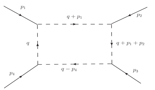
Figure 15: This diagram defines $\displaystyle W(p_{1},p_{2},p_{3},p_{4})$ in (275).

The expression for $\displaystyle{\tilde{S}}_{4}(p_{1},p_{2},p_{3},p_{4})$ can be somewhat simplified by noting that

$$W(p_{1},a,b,c)=W(p_{1},c,b,a),$$ (276)

so that

$${\tilde{S}}_{4}(p_{1},p_{2},p_{3},p_{4})=-2N_{B}\left(W(p_{1},p_{2},p_{3},p_{4})+W(p_{1},p_{2},p_{4},p_{3})+W(p_{1},p_{3},p_{2},p_{4})\right).$$ (277)

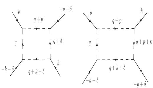
Figure 16: This diagram shows contributions to $\displaystyle{\tilde{S}}(p,-p+\delta,k,-k-\delta)$

In the rest of this subsubsection we will proceed to further simplify (277) in the kinematical regime of most interest to us, namely $\displaystyle{\tilde{S}}_{4}(p,-p+\delta,k,-k-\delta)$ in the limit $\displaystyle\delta\to 0$ (see Figure 16). It follows from (277) that

$$\begin{split}-\frac{1}{N_{B}}{\tilde{S}}_{4}(p,-p+\delta,k,-k-\delta)=&2W(p,-p+\delta,k,-k-\delta)+2W(p,-p+\delta,-k-\delta,k)\\ &+2W(p,k,-p+\delta,-k-\delta).\end{split}$$ (278)

The expressions on the first line of (278) blow up in the limit $\displaystyle\delta\to 0$, while the expression on the second line is finite in the same limit. We will first proceed to evaluate the expressions on the two lines separately, and then physically interpret the divergence as $\displaystyle\delta\to 0$ and explain how it is dealt with.

Let us first deal with the second line of (278). In this expression we can simply set $\displaystyle\delta=0$, obtaining

$$2\int\frac{d^{3}q}{(2\pi)^{3}}\frac{1}{q^{2}(q+p)^{2}(q+p+k)^{2}(q+k)^{2}}.$$ (279)

This integral is still rather complicated; however it simplifies in the limit that $\displaystyle\frac{|k|}{|p|}$ is small. In this limit we can separate the integral over $\displaystyle q$ into two balls and the rest. The first ball $\displaystyle B_{1}$ is given by $\displaystyle|q|<M|k|$. The second ball $\displaystyle B_{2}$ is the region $\displaystyle|p+q|<M|k|$. Here $\displaystyle M$ is a number chosen so that

$$1\ll M\ll\frac{|p|}{|k|}.$$ (280)

Let the contribution to the integral from points $\displaystyle q\in B_{1}$ be denoted by $\displaystyle C_{B}(p,k)$. The contribution to the integral from points $\displaystyle q$ in $\displaystyle B_{2}$ is then given by $\displaystyle C_{B}(-p,k)=C_{B}(p,-k)$. To leading order in the small $\displaystyle|k|$ limit we have

$$C_{B}(p,k)=\frac{2}{|k||p|^{4}}\left(\frac{1}{8}-\frac{1}{2\pi^{2}M}\right),$$ (281)

where we have used

$$\int\frac{d^{3}q}{(2\pi)^{3}}\frac{1}{q^{2}(q-p)^{2}}=\frac{1}{8|p|}.$$ (282)

On the other hand the contribution of the rest of space, $\displaystyle C_{R}(p,k)$ to this integral is

$$C_{R}(p,k)=\frac{4}{|k||p|^{4}}\left(\frac{1}{2\pi^{2}M}+{\cal O}(\frac{|k|}{|p|})\right).$$ (283)

Adding together the contributions of the two balls and the rest, we find that the second line of (278) is given by

$$\frac{1}{2|k||p|^{4}}\left(1+O\left(\frac{|k|}{|p|}\right)\right).$$ (284)

Let us now turn to the first line of (278). We have

$$\begin{split}&2W(p,-p+\delta,k,-k-\delta)+2W(p,-p+\delta,-k-\delta,k)\\ &=2\int\frac{d^{3}q}{(2\pi)^{3}}\frac{1}{q^{2}(\delta+q)^{2}(p+q)^{2}}\left(\frac{1}{(\delta+k+q)^{2}}+\frac{1}{(q-k)^{2}}\right)\\ &=2\int\frac{d^{3}q}{(2\pi)^{3}}\frac{1}{q^{2}(\delta+q)^{2}}\left(\frac{1}{(p+q)^{2}(\delta+k+q)^{2}}+\frac{1}{(p+q)^{2}(q-k)^{2}}-\frac{2}{|p||p-\delta||k||k+\delta|}\right)\\ &+\frac{1}{2|\delta|~{}|p||p-\delta||k||k+\delta|},\end{split}$$ (285)

where we have used (282) to obtain the last line of (285). The final integral in (285) is finite in the limit $\displaystyle\delta\to 0$; it follows that

$$\begin{split}&\lim_{\delta\to 0}\left(2W(p,-p+\delta,k,-k-\delta)+2W(p,-p+\delta,-k-\delta,k)-\frac{1}{2|\delta||p||p-\delta||k||k+\delta|}\right)\\ &=2\lim_{\delta\to 0}\int\frac{d^{3}q}{(2\pi)^{3}}\frac{1}{q^{2}(q+\delta)^{2}}\left(\frac{1}{(p+q)^{2}(k+q+\delta)^{2}}+\frac{1}{(p+q)^{2}(k-q)^{2}}-\frac{2}{|p||p-\delta||k||k+\delta|}\right).\\ \end{split}$$ (286)

As above we now explore the limit $\displaystyle|k|\ll|p|$. In this limit it is useful, as above, to view the integral in (286) as the sum of two integrals. In the first integral $\displaystyle q$ is contained in a ball of radius $\displaystyle M|k|$ centered around $\displaystyle q=0$, where $\displaystyle M$ obeys the inequality (280). In this region $\displaystyle|q|\ll|p|$ and we can simplify the integrand by Taylor expanding the integrand in a Taylor series expansion in $\displaystyle|q|/|p|$ as well as $\displaystyle|k|/|p|$. In the complement of the ball, on the other hand, $\displaystyle|k|/|q|$ is small so the integrand can be simplified by Taylor expanding in $\displaystyle|k|/|q|$ as well as $\displaystyle|k|/|p|$. As above it turns out that the contribution of the complement of the ball scales like $\displaystyle\frac{1}{M}$ and so can be ignored in the large $\displaystyle M$ limit of actual interest to us. We focus entirely on the contribution of the interior of the ball in what follows.

The first potential concern about the integral (286) is whether the limit $\displaystyle\delta\to 0$ is nonsingular. In order to address this concern we expand the integral in the second line of (286) in a Taylor series expansion in $\displaystyle\frac{1}{|p|}$. As $\displaystyle|\delta|$, $\displaystyle|q|$ and $\displaystyle|k|$ are all much less than $\displaystyle|p|$ in the interior of the ball, this Taylor expansion can be legitimately carried out inside the integral and we find that the integral (286) reduces to

$$\begin{split}&2\int\frac{d^{3}q}{(2\pi)^{3}}\frac{1}{p^{2}q^{2}(q+\delta)^{2}}\left(\frac{1}{(k+q+\delta)^{2}}+\frac{1}{(k-q)^{2}}-\frac{2}{|k||k+\delta|}\right)\\ &-\frac{4}{p^{4}}\int\frac{d^{3}q}{(2\pi)^{3}}\frac{q.p}{q^{2}(q+\delta)^{2}}\left(\frac{1}{(k+q+\delta)^{2}}+\frac{1}{(k-q)^{2}}\right)-\frac{p.\delta}{2p^{4}|\delta||k||k+\delta|}\\ &+4\int\frac{d^{3}q}{(2\pi)^{3}}\left(\frac{\frac{q^{2}}{p^{2}}-4\frac{(p\cdot q)^{2}}{p^{4}}}{(q^{2})^{2}(k+q)^{2}p^{2}}\right)+{\cal O}(1/|p|^{5}).\end{split}$$ (287)

In the first line of (LABEL:szi) we have collected all terms in the integrand of (286) of order $\displaystyle\frac{1}{|p|^{2}}$. Terms of order $\displaystyle\frac{1}{|p|^{3}}$ and order $\displaystyle\frac{1}{|p|^{4}}$, respectively, are collected on the second and third lines. All terms of higher order in $\displaystyle\frac{1}{|p|}$ are ignored.

Using the integrals

$$\begin{split}&\int\frac{d^{3}q}{(2\pi)^{3}}\frac{1}{q^{2}(q+p_{1})^{2}(q+p_{2})^{2}}=\frac{1}{|p_{1}||p_{2}||p_{1}-p_{2}|},\\ &\int\frac{d^{3}q}{(2\pi)^{3}}\frac{q_{\mu}}{q^{2}(q+\alpha)^{2}(q+\beta)^{2}}=\frac{1}{2}\left(a~{}\alpha_{\mu}+b~{}\beta_{\mu}\right),\\ &a=-\frac{1}{8|\alpha||\alpha-\beta|}\left(\frac{|\alpha|+|\beta|-|\alpha-\beta|}{|\alpha||\beta|+\alpha\cdot\beta}\right),\\ &b=-\frac{1}{8|\beta||\alpha-\beta|}\left(\frac{|\alpha|+|\beta|-|\alpha-\beta|}{|\alpha||\beta|+\alpha\cdot\beta}\right),\end{split}$$ (288)

it is easily verified that the first two lines of (LABEL:szi) simply vanish. This is a very important point; individual terms on the first line of (LABEL:szi) integrate to expressions proportional to $\displaystyle\frac{1}{|\delta|}$, and individual terms on the second line of (LABEL:szi) evaluate to expressions of the schematic form $\displaystyle\frac{\alpha\cdot\delta}{|\delta|}$; these terms all have singular $\displaystyle|\delta|\to 0$ limits. The fact that the first and second lines of (LABEL:szi) simply vanish implies that the $\displaystyle\delta\to 0$ limit in the integral (286) is well-defined.

The fourth line in (LABEL:szi) does not vanish. This integral is the sum of two terms. The first of these is an integral proportional to (282) and is easily evaluated. The second is proportional to the integral

$$\int\frac{d^{3}q}{(2\pi)^{3}}\frac{\frac{(p\cdot q)^{2}}{p^{4}}}{(q^{2})^{2}(k+q)^{2}p^{2}}$$ (289)

In order to evaluate this integral we first note that by symmetry

$$\int\frac{d^{3}q}{(2\pi)^{3}}\frac{q_{\mu}q_{\nu}}{(q^{2})^{2}(k+q)^{2}}=B_{0}(|k|)\delta_{\mu\nu}+B_{1}(|k|)\frac{k_{\mu}k_{\nu}}{k^{2}}.$$ (290)

A short calculation yields

$$B_{0}(|k|)=\frac{1}{32|k|},~{}~{}~{}B_{1}(|k|)=\frac{1}{32|k|}.$$ (291)

Putting everything together we find that the third line in (LABEL:szi) – and so our final result for the integral (286) up to terms of order $\displaystyle\frac{1}{|p|^{5}}$ – is

$$\frac{(p\cdot k)^{2}}{2k^{2}p^{6}}.$$ (292)

Adding this to (284) we obtain our final result which may be expressed as follows. Let us define

$${\tilde{S}}_{4}^{E}(p_{1}-\delta_{1}-\delta_{2},-p,\delta_{1},\delta_{2})={\tilde{S}}_{4}(p-\delta_{1}-\delta_{2},-p,\delta_{1},\delta_{2})-\frac{S_{3}(p-\delta_{1}-\delta_{2},-p,\delta_{1}+\delta_{2})S_{3}(\delta_{1},\delta_{2},-\delta_{1}-\delta_{2})}{S_{2}(\delta_{1}+\delta_{2})}.$$ (293)

It follows that

$${\tilde{S}}_{4}^{E}(p,-p+\delta,k,-k-\delta)=\left({\tilde{S}}_{4}(p,-p+\delta,k,-k-\delta)+\frac{1}{2|\delta||p||p-\delta||k||k+\delta|}\right).$$ (294)

Note that $\displaystyle{\tilde{S}}_{4}^{E}$ is simply the effective vertex that determines the leading large $\displaystyle N$ four point Green’s function of four $\displaystyle\sigma$ operators. We get the Green’s function by multiplying $\displaystyle{\tilde{S}}_{4}^{E}$ by

$$P=\prod_{i=1}^{4}\frac{1}{{\tilde{S}}_{2}(p_{i})}.$$ (295)

The final result of our computations is best worded in terms of $\displaystyle{\tilde{S}}_{4}^{E}$ and is

$$\begin{split}&\lim_{\delta\to 0}\frac{1}{N_{B}}\left({\tilde{S}}_{4}^{E}\right)=-\frac{1}{2}\frac{1}{|p|^{4}|k|}-\frac{1}{2}\frac{(p\cdot k)^{2}}{|p|^{6}k^{3}}+{\cal O}(1/|p|^{5}),\\ \end{split}$$ (296)

where the right-hand side is presented in a Taylor expansion in $\displaystyle\frac{|k|}{|p|}$, with all terms of the same homogeneity in $\displaystyle k$ being thought of as of the same order.

It follows that the Green’s function of four $\displaystyle\sigma$ operators is given by

$$\lim_{\delta\to 0}G_{4}^{0}(p,-p+\delta,k,-k-\delta)=-\frac{8^{4}}{N_{B}^{3}}\left(\frac{1}{2|k+p|}+\frac{1}{2|k-p|}-\frac{1}{2}\frac{|k|}{|p|^{2}}-\frac{1}{2}\frac{(p\cdot k)^{2}}{|p|^{4}|k|}+{\cal O}(k^{2}/p^{3})\right).$$ (297)

B.1.3 The quintic term

The fifth order term in the effective action is given by

$$\begin{split}&{\tilde{S}}_{5}(p_{1},p_{2},p_{3},p_{4})=2N_{B}\Bigg{(}H(p_{1},p_{2},p_{3},p_{4},p_{5})+H(p_{1},p_{2},p_{3},p_{5},p_{4})+H(p_{1},p_{2},p_{4},p_{3},p_{5})\\ &\qquad\qquad\qquad\qquad\qquad+H(p_{1},p_{2},p_{4},p_{5},p_{3})+H(p_{1},p_{2},p_{5},p_{3},p_{4})+H(p_{1},p_{2},p_{5},p_{4},p_{3})\\ &\qquad\qquad\qquad\qquad\qquad+H(p_{1},p_{3},p_{2},p_{4},p_{5})+H(p_{1},p_{3},p_{2},p_{5},p_{4})+H(p_{1},p_{4},p_{2},p_{3},p_{5})\\ &\qquad\qquad\qquad\qquad\qquad+H(p_{1},p_{4},p_{2},p_{5},p_{3})+H(p_{1},p_{5},p_{2},p_{3},p_{4})+H(p_{1},p_{5},p_{2},p_{4},p_{3})\Bigg{)}\end{split}$$ (298)

(one first finds 24 terms, but then uses ‘reflection symmetry’ of the graphs to simplify this to a sum of 12 terms with an additional factor of 2, as in the case of the quartic expression). Here (see figure 17)

$$H(p_{1},p_{2},p_{3},p_{4},p_{5})\equiv\int\frac{d^{3}q}{(2\pi)^{3}}\frac{1}{q^{2}(q+p_{1})^{2}(q+p_{1}+p_{2})^{2}(q-p_{4}-p_{5})^{2}(q-p_{5})^{2}}.$$ (299)

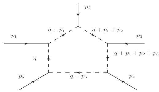
Figure 17: This diagram defines $\displaystyle H(p_{1},p_{2},p_{3},p_{4},p_{5})$ in (299). Note that by momentum conservation $\displaystyle p_{1}+p_{2}+p_{3}=-p_{4}-p_{5}.$

In the rest of this subsubsection we will proceed to simplify (LABEL:fi) in the kinematical regime of most interest to us, namely $\displaystyle{\tilde{S}}_{5}(p-\delta_{1}-\delta_{2}-\delta_{3},-p,\delta_{1},\delta_{2},\delta_{3})$ in the limit $\displaystyle\delta_{i}\to 0$ for all $\displaystyle i=1,2,3$. $\displaystyle{\tilde{S}}_{5}$ is highly singular in this limit. Note that on dimensional grounds $\displaystyle{\tilde{S}}_{5}$ scales like $\displaystyle(momentum)^{-7}$. For the physical purposes of interest to this paper, we are not interested in $\displaystyle{\tilde{S}}_{5}$ itself, but in the tree level 5 point function computed from the action formed from $\displaystyle{\tilde{S}}_{5}$, $\displaystyle{\tilde{S}}_{4}$, $\displaystyle{\tilde{S}}_{3}$ and the propagator derived from $\displaystyle{\tilde{S}}_{2}$. We expect this five point function to have a smooth limit as $\displaystyle\delta_{i}\to 0$.

The contribution of tree diagrams involving $\displaystyle{\tilde{S}}_{4}$, $\displaystyle{\tilde{S}}_{3}$ effectively renormalizes $\displaystyle{\tilde{S}}_{5}$ in an additive manner. Graphs with one $\displaystyle{\tilde{S}}_{4}$ vertex and one $\displaystyle{\tilde{S}}_{3}$ vertex contribute as follows. Define (see Figure 18)

$$J(p_{1},p_{2},p_{3},p_{4},p_{5})=-\frac{{\tilde{S}}_{3}(p_{1},p_{2},-(p_{1}+p_{2})){\tilde{S}}_{4}(p_{1}+p_{2},p_{3},p_{4},p_{5})}{{\tilde{S}}_{2}(p_{1}+p_{2})}.$$ (300)

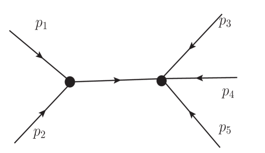
Figure 18: This diagram defines $\displaystyle J(p_{1},p_{2},p_{3},p_{4},p_{5})$ in (300).

Then the contribution of such mixed graphs to the effective value of $\displaystyle{\tilde{S}}_{5}$ is

$$\begin{split}&J(p_{1},p_{2},p_{3},p_{4},p_{5})+J(p_{1},p_{3},p_{2},p_{4},p_{5})+J(p_{1},p_{4},p_{3},p_{2},p_{5})+J(p_{1},p_{5},p_{3},p_{4},p_{2})\\ &+J(p_{3},p_{2},p_{1},p_{4},p_{5})+J(p_{4},p_{2},p_{3},p_{1},p_{5})+J(p_{5},p_{2},p_{3},p_{4},p_{1})+J(p_{3},p_{4},p_{1},p_{2},p_{5})\\ &+J(p_{3},p_{5},p_{1},p_{4},p_{2})+J(p_{4},p_{5},p_{3},p_{1},p_{2}).\\ \end{split}$$ (301)

In a similar manner, the contribution from tree graphs involving three cubic vertices is given as follows. Let us define (see Figure 19)

$$K(p_{1},p_{2},p_{3},p_{4},p_{5})=\frac{{\tilde{S}}_{3}(p_{1},p_{2}+p_{3},p_{4}+p_{5}){\tilde{S}}_{3}(p_{2},p_{3},-(p_{2}+p_{3})){\tilde{S}}_{3}(p_{4},p_{5},-(p_{4}+p_{5}))}{{\tilde{S}}_{2}(p_{2}+p_{3}){\tilde{S}}_{2}(p_{4}+p_{5})}.$$ (302)

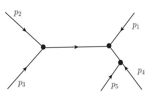
Figure 19: This diagram defines $\displaystyle K(p_{1},p_{2},p_{3},p_{4},p_{5})$ in (302).

The effective additive shift to $\displaystyle{\tilde{S}_{5}}$ from such graphs is given by

$$\begin{split}&K(p_{1},p_{2},p_{3},p_{4},p_{5})+K(p_{1},p_{2},p_{4},p_{3},p_{5})+K(p_{1},p_{2},p_{5},p_{3},p_{4})+\\ &K(p_{2},p_{1},p_{3},p_{4},p_{5})+K(p_{2},p_{1},p_{4},p_{3},p_{5})+K(p_{2},p_{1},p_{5},p_{3},p_{4})+\\ &K(p_{3},p_{2},p_{1},p_{4},p_{5})+K(p_{3},p_{2},p_{4},p_{1},p_{5})+K(p_{3},p_{2},p_{5},p_{1},p_{4})+\\ &K(p_{4},p_{2},p_{3},p_{1},p_{5})+K(p_{4},p_{2},p_{1},p_{3},p_{5})+K(p_{4},p_{2},p_{5},p_{3},p_{1})+\\ &K(p_{5},p_{2},p_{3},p_{4},p_{1})+K(p_{5},p_{2},p_{4},p_{3},p_{1})+K(p_{5},p_{2},p_{1},p_{3},p_{4}).\\ \end{split}$$ (303)

The final effective five point function, $\displaystyle{\tilde{S}}^{E}_{5}$ is obtained by adding (301) and (303) to $\displaystyle{\tilde{S}}_{5}$. In order to obtain the 5 point Green’s function for $\displaystyle\sigma$ we must then multiply this effective five point function by

$$P=\prod_{i=1}^{5}\frac{1}{{\tilde{S}}_{2}(p_{i})}.$$ (304)

B.1.4 $\displaystyle SO(N)$

Throughout this subsection we have so far assumed that the scalar fields in the initial action (11) are all complex. All our results for the effective action as a function of $\displaystyle\sigma$ are easily modified to the case that the fields $\displaystyle\phi$ are real (so that we have an $\displaystyle SO(N_{B})$ symmetry rather than a unitary symmetry). If we replace the second line in (11) by the action

$$S=\int d^{3}x\left(\frac{1}{2}\partial_{\mu}\phi\partial^{\mu}\phi+\sigma\phi^{2}\right)$$ (305)

for real fields $\displaystyle\phi_{m}$, we find that

$${\tilde{S}}_{n}^{SO(N)}=2^{n-1}{\tilde{S}}_{n}^{SU(N)}.$$ (306)

B.2 First subleading corrections to the quadratic and cubic vertices

In this subsection we continue to work with the critical boson theory at $\displaystyle\lambda_{B}=0$. Using the explicit results of the previous subsection, we proceed to evaluate the first corrections, in an expansion in $\displaystyle\frac{1}{N_{B}}$, to the effective action for $\displaystyle\sigma$ at quadratic order, and study the same correction at cubic order. Our explicit evaluation of the quadratic correction allows us to compute the anomalous dimension of $\displaystyle\sigma$ at order $\displaystyle\frac{1}{N_{B}}$; we find agreement with results previously computed in the literature. This serves as a check of the formalism developed in this paper. At cubic order we find a formal expression for the divergent part of the correction to the cubic effective action for $\displaystyle\sigma$. The expressions we derive will allow us to demonstrate that the constant part of the $\displaystyle\beta$ function for $\displaystyle x_{6}$ – computed earlier in this paper – indeed vanishes for the regular boson theory at $\displaystyle\lambda_{B}=0$ as it must on physical grounds, providing an additional check of the results of this paper.

B.2.1 Anomalous dimension of $\displaystyle\sigma$ at first subleading order in $\displaystyle\frac{1}{N}$

It is useful to think of $\displaystyle S_{eff}(\sigma)$ as a classical action which then receives loop corrections; the loop expansion parameter is $\displaystyle\frac{1}{N_{B}}$. At quadratic order it is given by

$$S_{eff}(\sigma)=\frac{1}{2}\int\frac{d^{3}p}{(2\pi)^{3}}{\tilde{S}}_{2}(p)\sigma(p)\sigma(-p)=\frac{1}{2}\int\frac{d^{3}p}{(2\pi)^{3}}(\frac{-N_{B}}{8|p|})\sigma(p)\sigma(-p).$$ (307)

Figure 20: One of the three one loop corrections to the quadratic effective action for $\displaystyle\sigma$.

The quantum effective action for $\displaystyle\sigma$ includes the classical term (307) together with quantum corrections. At first subleading order in $\displaystyle\frac{1}{N_{B}}$ it is given by

$$S_{eff}(\sigma)=\frac{1}{2}\int\frac{d^{3}p}{(2\pi)^{3}}\left({\tilde{S}}_{2}(p)+\delta S_{2}\right)\sigma(p)\sigma(-p)=\frac{1}{2}\int\frac{d^{3}p}{(2\pi)^{3}}(\frac{-N_{B}}{8|p|}+\delta S_{2}(p))\sigma(p)\sigma(-p),$$ (308)

where the self energy correction $\displaystyle\delta S_{2}$ receives contributions from three distinct one loop graphs. The first graph describes a $\displaystyle\sigma$ ‘particle’ splitting into two via a cubic vertex (see figure 20); the resultant ‘particles’ then rejoin into a single $\displaystyle\sigma$ particle through another cubic vertex. We call this contribution $\displaystyle A_{3}(p)$ below. The remaining two graphs are both tadpole type graphs. The first of these is the contribution of a four point vertex with two its legs sewn together. The second graph has the two external $\displaystyle\sigma$ lines ‘colliding’ to form a single internal sigma propagator, whose other end meets a cubic vertex. The remaining two lines in the cubic vertex contract. We denote the combined contribution of these two graphs as $\displaystyle A_{4}(p)$ below (the graphs are similar to those of figure 4 above). We find

$$\begin{split}\delta S_{2}(p)&=\left(A_{3}(p)+A_{4}(p)\right),\\ A_{3}(p)&=-\frac{1}{2}\int\frac{d^{3}q}{(2\pi)^{3}}\frac{S_{3}(p,q,-(p+q))S_{3}(-p,-q,(p+q))}{S_{2}(q)S_{2}(p+q)}=\frac{1}{2\pi^{2}|p|},\\ A_{4}(p)&=\frac{1}{2}\int\frac{d^{3}q}{(2\pi)^{3}}\frac{\lim_{\delta\to 0}\left(S_{4}(p,-p+\delta,q,-q-\delta)-\frac{S_{3}(p,-p-\delta,\delta)S_{3}(q,-q-\delta,\delta)}{S_{2}(\delta)}\right)}{S_{2}(q)}\\ &=\frac{1}{2}\int\frac{d^{3}q}{(2\pi)^{3}}\lim_{\delta\to 0}\left({\tilde{S}}^{E}_{4}(p,-p+\delta,q,-q-\delta)\right)\\ &=\frac{4}{3\pi^{2}|p|}\left(\alpha\ln(\frac{\Lambda}{|p|})+\beta\right).\end{split}$$ (309)

The explicit result for $\displaystyle A_{3}(p)$ above is obtained by substituting the explicit expression for $\displaystyle{\tilde{S}}_{3}(p_{1},p_{2},p_{3})$ and using (282). As we do not have an explicit expression for $\displaystyle{\tilde{S}}_{4}(p_{1},p_{2},p_{3},p_{4})$, we evaluate the integral $\displaystyle A_{4}(p)$ in a more indirect manner. Dimensional analysis together with power counting imply that $\displaystyle A_{4}(p)$ takes the form reported in the last line of (309), where $\displaystyle\Lambda$ is a UV cutoff and $\displaystyle\alpha$ and $\displaystyle\beta$ are pure numbers. The number $\displaystyle\beta$ depends on the precise definition of the UV cutoff. On the other hand the number $\displaystyle\alpha$ is universal (in the sense that it is insensitive to the details of the UV cutoff). In order to compute $\displaystyle\alpha$ we need only compute the coefficient of $\displaystyle\ln(\Lambda)$ in $\displaystyle A_{4}$. By power counting, only those terms that scale like $\displaystyle\frac{1}{q^{4}}$ in the numerator of the integrand in the second last line of (309) give rise to a logarithmic divergence in $\displaystyle A_{4}(p)$. However all such terms were listed in (296). Substituting (296) into the last line of (309) we find

$$\begin{split}A_{4}(p)&=\frac{1}{2}\left(\int\frac{d^{3}k}{(2\pi)^{3}}\frac{-\frac{1}{2}\frac{1}{|k|^{4}|p|}-\frac{1}{2}\frac{(p\cdot k)^{2}}{|k|^{6}p^{3}}}{-\frac{1}{8|k|}}+...\right)\\ &=\frac{4}{3\pi^{2}|p|}\left(\int\frac{dk}{k}+...\right)=\frac{4}{3\pi^{2}|p|}\ln(\Lambda)+\cdots\\ \end{split}$$ (310)

The terms $\displaystyle\cdots$ denote those parts of the integrand whose contribution to the integral is finite in the UV. In going from the first to the second line of (310) we have performed the angular integral and used the fact that $\displaystyle\cos^{2}(\theta)$ averages to $\displaystyle\frac{1}{3}$.

It follows that $\displaystyle\alpha=1$, so that

$${\tilde{S}}_{2}(p)+\delta S_{2}(p)=-\frac{N_{B}}{8|p|}\left(1+\frac{32}{3\pi^{2}N_{B}}\ln\left(\frac{|p|}{|\Lambda|}\right)+\frac{c}{N_{B}}\right)=-(1+\frac{c}{N_{B}})\frac{N_{B}}{8|p|}\left(\frac{\Lambda}{|p|}\right)^{-\frac{32}{3\pi^{2}N_{B}}},$$ (311)

where $\displaystyle c$ is a number of order unity that we will not need.

The Green’s function for $\displaystyle\sigma$ is given by inverting the quantum effective action for $\displaystyle\sigma$, which gives

$$G_{2}(p)\propto-8|p|\left(\frac{\Lambda}{|p|}\right)^{\frac{32}{3\pi^{2}N_{B}}}.$$ (312)

It follows that the scaling dimension of $\displaystyle\sigma$ is given at first subleading order in $\displaystyle\frac{1}{N_{B}}$ by

$$\Delta_{\sigma}=2-\frac{16}{3\pi^{2}N_{B}}.$$ (315)

We have so far focused on the case of the $\displaystyle U(N_{B})$ theory, in which the basic scalar fields are all complex. The analogous results for the $\displaystyle SO(N_{B})$ theory are, however, easily obtained. The first line of (309) still applies to the $\displaystyle SO(N_{B})$ theory. The second and fourth line of that equation also apply provided we use the values of $\displaystyle S_{4}$, $\displaystyle S_{3}$, and $\displaystyle S_{2}$ appropriate to the $\displaystyle SO(N_{B})$ theory. Using (306) it follows that

$$A_{3}(p)^{SO(N_{B})}=4A_{3}(p)^{U(N_{B})},~{}~{}~{}~{}A_{4}(p)^{SO(N_{B})}=4A_{4}(p)^{U(N_{B})}.$$ (316)

It follows that

$$\delta S_{2}^{SO(N_{B})}(p)=4\delta S_{2}^{U(N_{B})}(p).$$ (317)

On the other hand (306) asserts that

$$S_{2}^{SO(N_{B})}(p)=2S_{2}^{U(N_{B})}(p).$$ (318)

As the anomalous dimension of $\displaystyle\sigma$ is determined by the relative factor between $\displaystyle\delta S_{2}$ and $\displaystyle S_{2}$, it follows that the anomalous dimension of $\displaystyle\sigma$ in the $\displaystyle SO(N_{B})$ theory is twice the anomalous dimension in the $\displaystyle U(N_{B})$ theory, so that the dimension of $\displaystyle\sigma$ in the $\displaystyle SO(N_{B})$ theory is given by

$$\Delta_{\sigma}=2-\frac{32}{3\pi^{2}N_{B}}.$$ (319)

B.2.2 Correction to the divergent part of the Green’s function $\displaystyle G_{3}$ at first order in $\displaystyle\frac{1}{N}$

As in the previous section we now proceed to compute the first correction to $\displaystyle{\tilde{S}_{3}}$ in the $\displaystyle\frac{1}{N_{B}}$ expansion. Focusing on terms at cubic order, the $\displaystyle\sigma$ effective action takes the schematic form

$$S_{eff}(\sigma)=\left({\tilde{S}}_{3}+\delta S_{3}\right)\sigma^{3},$$ (320)

where $\displaystyle{\tilde{S}}_{3}$ was listed in (272) and

$$\begin{split}\delta S_{3}(q_{1},q_{2},q_{3})&=\int\frac{d^{3}q}{(2\pi)^{3}}\frac{{\tilde{S}}_{3}(q_{1},q,-q-q_{1}){\tilde{S}}_{3}(q_{2},-q+q_{3},q+q_{1}){\tilde{S}}_{3}(q_{3},-q,q-q_{3})}{{\tilde{S}}_{2}(q+q_{1}){\tilde{S}}_{2}(q-q_{3}){\tilde{S}}_{2}(q)}\\ &\qquad-\frac{3}{2}\int\frac{d^{3}q}{(2\pi)^{3}}\frac{{\tilde{S}}_{4}(q_{1},q_{2},-q+q_{3},q){\tilde{S}}_{3}(q-q_{3},-q,q_{3})}{{\tilde{S}}_{2}(q){\tilde{S}}_{2}(q-q_{3})}\\ &\qquad+\frac{1}{2}\int\frac{d^{3}q}{(2\pi)^{3}}\frac{{\tilde{S}}_{5}(q_{1},q_{2},q_{3},q,-q)}{{\tilde{S}}_{2}(q)}\end{split}$$ (321)

(where the second line should be symmetrized over the three external momenta).

Accurate to first subleading order, the three-point function of three $\displaystyle\sigma$ operators is given by the formula

$$\langle\sigma(q_{1})\sigma(q_{2})\sigma(q_{3})\rangle=-\prod_{i=1}^{3}\left({\tilde{S}_{2}}(q_{i})+\delta S_{2}(q_{i})\right)^{-1}\left({\tilde{S}_{3}}(q_{1},q_{2},q_{3})+\delta S_{3}(q_{1},q_{2},q_{3})\right).$$ (322)

It follows that $\displaystyle\delta G_{3}$, the first correction to $\displaystyle{\tilde{G}}_{3}$ (the leading order three point function for $\displaystyle\sigma$) in an expansion in $\displaystyle\frac{1}{N_{B}}$, is given by

$$\delta G_{3}=\frac{1}{{\tilde{S}}_{2}(q_{1}){\tilde{S}}_{2}(q_{2}){\tilde{S}}_{2}(q_{3})}\left(-\delta S_{3}+{\tilde{S}}_{3}\sum_{i=1}^{3}\frac{\delta{S}_{2}(q_{i})}{{\tilde{S}}_{2}(q_{i})}\right).$$ (323)

Joining everything together we have

$$\begin{split}&\delta G_{3}(q_{1},q_{2},q_{3})\\ &=-\frac{1}{{\tilde{S}}_{2}(q_{1}){\tilde{S}}_{2}(q_{2}){\tilde{S}}_{2}(q_{3})}\bigg{(}\int\frac{d^{3}q}{(2\pi)^{3}}\frac{{\tilde{S}}_{3}(q_{1},q,-q-q_{1}){\tilde{S}}_{3}(q_{2},-q+q_{3},q+q_{1}){\tilde{S}}_{3}(q_{3},-q,q-q_{3})}{{\tilde{S}}_{2}(q+q_{1}){\tilde{S}}_{2}(q-q_{3}){\tilde{S}}_{2}(q)}\\ &\qquad\qquad-\frac{3}{2}\int\frac{d^{3}q}{(2\pi)^{3}}\frac{{\tilde{S}}_{4}(q_{1},q_{2},-q+q_{3},q){\tilde{S}}_{3}(q-q_{3},-q,q_{3})}{{\tilde{S}}_{2}(q){\tilde{S}}_{2}(q-q_{3})}\\ &\qquad\qquad-\frac{3}{2}\int\frac{d^{3}q}{(2\pi)^{3}}\frac{{\tilde{S}}_{4}(q_{3},q,-q,q_{1}+q_{2}){\tilde{S}}_{3}(-(q_{1}+q_{2}),q_{1},q_{2})}{{\tilde{S}}_{2}(q){\tilde{S}}_{2}(q_{1}+q_{2})}\\ &\qquad\qquad+\frac{3}{2}\int\frac{d^{3}q}{(2\pi)^{3}}\frac{{\tilde{S}}_{3}(q_{1},q_{2},q_{3}){\tilde{S}}_{3}(q_{3},q,q-q_{3}){\tilde{S}}_{3}(q,q_{3},q-q_{3})}{{\tilde{S}}_{2}(q_{3}){\tilde{S}}_{2}(q){\tilde{S}}_{2}(q-q_{3})}\\ &\qquad\qquad+\frac{1}{2}\int\frac{d^{3}q}{(2\pi)^{3}}\frac{{\tilde{S}}_{5}(q_{1},q_{2},q_{3},q,-q)}{{\tilde{S}}_{2}(q)}\bigg{)}\end{split}$$ (324)

(where the middle three lines should be symmetrized over the three external momenta). The third and fourth lines in (324) account for the second term (proportional to $\displaystyle\delta S_{2}$) in (323).

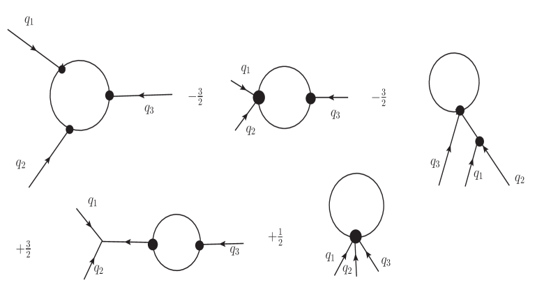
Figure 21: Contributions to the effective action (324).

The different contributions to (324) together with their symmetry factors are expressed in terms of graphs in figure 21.

The value of the parameter $\displaystyle r_{B}$ (see (LABEL:thptdet)) at $\displaystyle\lambda_{B}=0$ may be obtained by evaluating the terms in (324) that are proportional to $\displaystyle\ln(\Lambda)$. More directly the part of (324) that is proportional to $\displaystyle\ln(\Lambda)$ should be identified with the negative of the third line in (109).

The equation (323) is slightly formal because the expressions presented in (324) for $\displaystyle\delta S_{3}$ are expressed in terms of quite formidable integrals that have not been explicitly evaluated. Fortunately we will not need explicit expressions for the relevant expressions; the formal expression (324) will prove sufficient for our purposes below.

B.2.3 Vanishing of the $\displaystyle x_{6}$ independent piece of the $\displaystyle\beta$ function at $\displaystyle x_{6}=0$

The beta function (132) has three distinct kinds of contributions. One contribution, proportional to $\displaystyle\delta^{\prime}_{B}$, has its origins in the anomalous dimension of the $\displaystyle\zeta$ field. This anomalous dimension vanishes in the limit $\displaystyle\lambda_{B}=0$ – the limit of interest in this section. The second contribution – proportional to $\displaystyle{\tilde{g}}_{3}$ – has its origin in the $\displaystyle 1/N_{B}$ correction to the correlator of 3 $\displaystyle\sigma$ fields. This piece was computed in the previous subsection; as explained above it is determined by the coefficient of $\displaystyle\ln(\Lambda)$ in (323) above. The last contribution comes from the coefficient of the $\displaystyle\ln(\Lambda)$ terms in the graphs reported in (127), i.e. from the computation of $\displaystyle S^{IPI}(\zeta)-S^{eff}(\zeta)$.

In this subsection we will demonstrate that the second and third contributions described in the paragraph above cancel each other when $\displaystyle x_{6}=0$ (recall that we assume $\displaystyle\lambda_{B}=0$ throughout this section). In order to demonstrate cancellation we will not have to evaluate any integrals - it turns out that the cancellation happens at the formal level of unevaluated integrals.

As we have mentioned above, the second contribution to the $\displaystyle\beta$ function has already been listed in (324) in terms of integrals involving the vertex factors $\displaystyle S_{2}$, $\displaystyle S_{3}$, $\displaystyle S_{4}$ and $\displaystyle S_{5}$. In order to demonstrate cancellation we simply rewrite the integrals in (127) at $\displaystyle x_{6}=0$ and check that the resulting expressions cancel those listed in (324) term by term. Terms involving only the vertices $\displaystyle{\tilde{G}}_{3}$ and $\displaystyle{\tilde{G}}_{4}$ can be rewritten in terms of $\displaystyle{\tilde{S}_{3}}$, $\displaystyle{\tilde{S}}_{4}$, and $\displaystyle{\tilde{S}_{2}}$ in a quite straightforward manner; we find

$$\begin{split}&\int\frac{d^{3}q}{(2\pi)^{3}}\frac{G_{3}^{0}(q_{1},q,-q-q_{1})G_{3}^{0}(q_{2},-q+q_{3},q+q_{1})G_{3}^{0}(q_{3},-q,q-q_{3})}{G_{2}^{0}(q_{1})G_{2}^{0}(q_{2})G_{2}^{0}(q_{3})G_{2}^{0}(q+q_{1})G_{2}^{0}(q-q_{3})G_{2}^{0}(q)}\\ &\qquad=-\int\frac{d^{3}q}{(2\pi)^{3}}\frac{{\tilde{S}}_{3}(q_{1},q,-q-q_{1}){\tilde{S}}_{3}(q_{2},-q+q_{3},q+q_{1}){\tilde{S}}_{3}(q_{3},-q,q-q_{3})}{{\tilde{S}}_{2}(q+q_{1}){\tilde{S}}_{2}(q-q_{3}){\tilde{S}}_{2}(q)},\end{split}$$ (325)

$$\begin{split}&\int\frac{d^{3}q}{(2\pi)^{3}}\frac{G_{4}^{0}(q_{1},q_{2},-q+q_{3},q)G_{3}^{0}(q-q_{3},-q,q_{3})}{G_{2}^{0}(q_{1})G_{2}^{0}(q_{2})G_{2}^{0}(q_{3})G_{2}^{0}(q)G_{2}^{0}(q-q_{3})}\\ &=\int\frac{d^{3}q}{(2\pi)^{3}}\frac{{\tilde{S}}_{4}(q_{1},q_{2},-q+q_{3},q){\tilde{S}}_{3}(q-q_{3},-q,q_{3})}{{\tilde{S}}_{2}(q){\tilde{S}}_{2}(q-q_{3})}\\ &\qquad-\int\frac{d^{3}q}{(2\pi)^{3}}\frac{{\tilde{S}}_{3}(q_{1},q_{2},-(q_{1}+q_{2})){\tilde{S}}_{3}(q-q_{3},-q,q_{3}){\tilde{S}}_{3}(q-q_{3},-q,q_{3})}{{\tilde{S}}_{2}(q_{1}+q_{2}){\tilde{S}}_{2}(q){\tilde{S}}_{2}(q-q_{3})}\\ &\qquad-2\int\frac{d^{3}q}{(2\pi)^{3}}\frac{{\tilde{S}}_{3}(q_{1},q,-q-q_{1}){\tilde{S}}_{3}(q_{2},-q+q_{3},q+q_{1}){\tilde{S}}_{3}(q_{3},-q,q-q_{3})}{{\tilde{S}}_{2}(q+q_{1}){\tilde{S}}_{2}(q-q_{3}){\tilde{S}}_{2}(q)}.\end{split}$$ (326)

The terms involving $\displaystyle{\tilde{G}}_{5}$ are more delicate, and require considerable care with signs to accurately keep track of. We find

$$\begin{split}&\int\frac{d^{3}q}{(2\pi)^{3}}\frac{G_{5}^{0}(q_{1},q_{2},q_{3},q,-q)}{G_{2}^{0}(q_{1})G_{2}^{0}(q_{2})G_{2}^{0}(q_{3})G_{2}^{0}(q)}\\ &=-\int\frac{d^{3}q}{(2\pi)^{3}}\frac{{\tilde{S}}_{5}(q_{1},q_{2},q_{3},q,-q)}{{\tilde{S}}_{2}(q)}+6\int\frac{d^{3}q}{(2\pi)^{3}}\frac{{\tilde{S}}_{4}(q_{1},q_{2},-q+q_{3},q){\tilde{S}}_{3}(q-q_{3},-q,q_{3})}{{\tilde{S}}_{2}(q){\tilde{S}}_{2}(q-q_{3})}\\ &\qquad+3\int\frac{d^{3}q}{(2\pi)^{3}}\frac{{\tilde{S}}_{4}(q_{3},q,-q,q_{1}+q_{2}){\tilde{S}}_{3}(-(q_{1}+q_{2}),q_{1},q_{2})}{{\tilde{S}}_{2}(q){\tilde{S}}_{2}(q_{1}+q_{2})}\\ &\qquad-6\int\frac{d^{3}q}{(2\pi)^{3}}\frac{{\tilde{S}}_{3}(q_{1},q_{2},-(q_{1}+q_{2})){\tilde{S}}_{3}(q-q_{3},-q,q_{3}){\tilde{S}}_{3}(q-q_{3},-q,q_{3})}{{\tilde{S}}_{2}(q_{1}+q_{2}){\tilde{S}}_{2}(q){\tilde{S}}_{2}(q-q_{3})}\\ &\qquad-6\int\frac{d^{3}q}{(2\pi)^{3}}\frac{{\tilde{S}}_{3}(q_{1},q,-q-q_{1}){\tilde{S}}_{3}(q_{2},-q+q_{3},q+q_{1}){\tilde{S}}_{3}(q_{3},-q,q-q_{3})}{{\tilde{S}}_{2}(q+q_{1}){\tilde{S}}_{2}(q-q_{3}){\tilde{S}}_{2}(q)}.\end{split}$$ (327)

In the expressions (327), various factors of $\displaystyle 3$ and $\displaystyle 6$ should be thought of as different terms leading to same kind of integral. Adding the expressions (325), (326) and (327) together we find that the net expression for the third contribution (terms in $\displaystyle S^{1PI}-S^{eff}$) is

$$\begin{split}&\int\frac{d^{3}q}{(2\pi)^{3}}\frac{G_{3}^{0}(q_{1},q,-q-q_{1})G_{3}^{0}(q_{2},-q+q_{3},q+q_{1})G_{3}^{0}(q_{3},-q,q-q_{3})}{G_{2}^{0}(q+q_{1})G_{2}^{0}(q-q_{3})G_{2}^{0}(q)}\\ &-\frac{3}{2}\int\frac{d^{3}q}{(2\pi)^{3}}\frac{G_{4}^{0}(q_{1},q_{2},-q+q_{3},q)G_{3}^{0}(q-q_{3},-q,q_{3})}{G_{2}^{0}(q)G_{2}^{0}(q-q_{3})}+\frac{1}{2}\int\frac{d^{3}q}{(2\pi)^{3}}\frac{G_{5}^{0}(q_{1},q_{2},q_{3},q,-q)}{G_{2}^{0}(q)}\\ &=-\frac{1}{{\tilde{S}}_{2}(q_{1}){\tilde{S}}_{2}(q_{2}){\tilde{S}}_{2}(q_{3})}\bigg{(}-\int\frac{d^{3}q}{(2\pi)^{3}}\frac{{\tilde{S}}_{3}(q_{1},q,-q-q_{1}){\tilde{S}}_{3}(q_{2},-q+q_{3},q+q_{1}){\tilde{S}}_{3}(q_{3},-q,q-q_{3})}{{\tilde{S}}_{2}(q+q_{1}){\tilde{S}}_{2}(q-q_{3}){\tilde{S}}_{2}(q)}\\ &\qquad+\frac{3}{2}\int\frac{d^{3}q}{(2\pi)^{3}}\frac{{\tilde{S}}_{4}(q_{1},q_{2},-q+q_{3},q){\tilde{S}}_{3}(q-q_{3},-q,q_{3})}{{\tilde{S}}_{2}(q){\tilde{S}}_{2}(q-q_{3})}\\ &\qquad+\frac{3}{2}\int\frac{d^{3}q}{(2\pi)^{3}}\frac{{\tilde{S}}_{4}(q_{3},q,-q,q_{1}+q_{2}){\tilde{S}}_{3}(-(q_{1}+q_{2}),q_{1},q_{2})}{{\tilde{S}}_{2}(q){\tilde{S}}_{2}(q_{1}+q_{2})}\\ &\qquad-\frac{3}{2}\int\frac{d^{3}q}{(2\pi)^{3}}\frac{{\tilde{S}}_{3}(q_{1},q_{2},-(q_{1}+q_{2})){\tilde{S}}_{3}(q-q_{3},-q,q_{3}){\tilde{S}}_{3}(q-q_{3},-q,q_{3})}{{\tilde{S}}_{2}(q_{1}+q_{2}){\tilde{S}}_{2}(q){\tilde{S}}_{2}(q-q_{3})}\\ &\qquad-\frac{1}{2}\int\frac{d^{3}q}{(2\pi)^{3}}\frac{{\tilde{S}}_{5}(q_{1},q_{2},q_{3},q,-q)}{{\tilde{S}}_{2}(q)}\bigg{)}\\ &=\delta G_{3}.\end{split}$$ (328)

The fact that $\displaystyle S^{1PI}-S^{eff}$ equals $\displaystyle\delta G_{3}$ establishes that the contribution to $\displaystyle S^{1PI}$ from the correction to $\displaystyle G_{3}$ exactly cancels the loop contributions to $\displaystyle S^{1PI}$ at $\displaystyle x_{6}=0$. It follows that the $\displaystyle\beta$ function vanishes at $\displaystyle x_{6}=0$.

Of course the vanishing of this $\displaystyle\beta$ function is obvious on physical grounds (a free theory does not have a $\displaystyle\beta$ function). However the fact that this works out algebraically within our formalism is a consistency check of the formulae presented in this paper.

Appendix C Correlators for free fermions

In this Appendix we present computations of the two, three and (the connected part of) four point functions of the operator $\displaystyle J_{0}$ in the free fermion theory.

Recall that

$$J_{0}=\frac{4\pi{\bar{\psi}}\psi}{{\tilde{\kappa}}_{F}}.$$ (329)

It follows that in the limit $\displaystyle{\tilde{\kappa}}_{F}\to\infty$ of interest to this Appendix, the $\displaystyle n$ point functions of $\displaystyle J_{0}$ are given by $\displaystyle(\frac{4\pi}{{\tilde{\kappa}}_{F}})^{n}$ times the Wick contractions of $\displaystyle n$ copies of $\displaystyle{\bar{\psi}}\psi$. The Wick contractions are very easy to compute at arbitrary values of $\displaystyle N_{F}$. We now proceed to study two, three and four point functions in turn. We follow the same conventions as in Jain:2014nza . The two point function is given by

$$\langle J^{F}_{0}(q)J^{F}_{0}(-q^{\prime})\rangle=(2\pi)^{3}\delta^{3}(q-q^{\prime})N_{F}\left(\frac{4\pi}{{\tilde{\kappa}_{F}}}\right)^{2}\mathrm{Tr}\left(\int\frac{d^{d}q}{(2\pi)^{d}}\left(\frac{\not{q}\left(\not{q}+\not{p}\right)}{q^{2}(q+p)^{2}}\right)\right),$$ (330)

where $\displaystyle d=3$. The integral on the right-hand side of (330) is linearly divergent; we give it meaning by using dimensional regularization. Using $\displaystyle\mathrm{Tr}\left(\gamma^{\mu}\gamma^{\nu}\right)=2\eta^{\mu\nu}$, we find that within the dimensional regularization scheme

$$\begin{split}&\int\frac{d^{d}q}{(2\pi)^{d}}\left(\frac{{\rm Tr}(\not{q}\left(\not{q}+\not{p})\right)}{q^{2}(q+p)^{2}}\right)=-\int\frac{d^{d}q}{(2\pi)^{d}}\left(\frac{p^{2}}{(p+q)^{2}q^{2}}-\frac{1}{q^{2}}-\frac{1}{(p+q)^{2}}\right)\\ &\qquad=-\int\frac{d^{d}q}{(2\pi)^{d}}\left(\frac{p^{2}}{(p+q)^{2}q^{2}}-\frac{2}{q^{2}}\right)=-\frac{|p|}{8}.\end{split}$$ (331)

We have used the fact that in dimensional regularization

$$\begin{split}\int\frac{d^{d}q}{(2\pi)^{d}}\frac{1}{q^{2}}&=\int\frac{d^{d}q}{(2\pi)^{d}}\frac{1}{(q+p)^{2}}=0,\end{split}$$ (332)

and the convergent integral (282). It follows that

$$\langle J^{F}_{0}(q)J^{F}_{0}(-q^{\prime})\rangle=(2\pi)^{3}\delta^{3}(q-q^{\prime})\frac{(-2N_{F})\pi^{2}|q|}{{\tilde{\kappa}}_{F}^{2}}.$$ (333)

Equation (333) – which is accurate in the limit $\displaystyle{\tilde{\kappa}_{F}}\to\infty$ but at all values of $\displaystyle N_{F}$ – matches perfectly with (48).

The three point function of three $\displaystyle J_{0}^{F}$ operators simply vanishes. This fact can be seen algebraically from the fact that the diagram that computes this correlator is proportional to

$$\int\frac{d^{3}q}{(2\pi)^{3}}\frac{\epsilon_{\mu\nu\rho}q^{\mu}(p_{1}+q)^{\nu}(-p_{2}+q)^{\rho}}{q^{2}(p_{1}+q)^{2}(q-p_{3})^{2}}.$$ (334)

But clearly

$$\int\frac{d^{3}q}{(2\pi)^{3}}\frac{q^{\mu}}{q^{2}(p_{1}+q)^{2}(q-p_{3})^{2}}=ap_{1}^{\mu}+bp_{3}^{\mu},$$ (335)

where $\displaystyle a$ and $\displaystyle b$ are scalar functions of $\displaystyle p_{1}$ and $\displaystyle p_{2}$. Substituting (335) into (334) we see that the three point function of three $\displaystyle J_{0}^{F}$ operators vanishes.

The vanishing of the three point function could have been anticipated as follows. Recall that parity is a symmetry of the free fermion theory, and that $\displaystyle J_{0}^{F}$ is odd under a parity transformation. It follows that the three point function must also be odd under parity. The position dependence of the three point function of three $\displaystyle J_{0}^{F}$ operators, however, is completely fixed by conformal invariance to a functional form that is even under parity transformations of the three coordinates. It follows that the three point function must vanish.

Finally let us turn to the four point function (51). The function $\displaystyle G^{0}_{4}(p_{1},p_{2},p_{3},p_{4})$ defined in that equation is given by

$$\begin{split}G^{0}_{4}(p_{1},p_{2},p_{3},p_{4})&=N_{F}\left(\frac{4\pi}{{\tilde{\kappa}_{F}}}\right)^{4}\Bigg{(}Y(p_{1},p_{2},p_{3},p_{4})+Y(p_{1},p_{2},p_{4},p_{3})+Y(p_{1},p_{4},p_{3},p_{2})\\ &+Y(p_{1},p_{4},p_{2},p_{3})+Y(p_{1},p_{3},p_{4},p_{2})+Y(p_{1},p_{3},p_{2},p_{4})\Bigg{)},\end{split}$$ (336)

where

$$\begin{split}Y(p_{1},p_{2},p_{3},p_{4})&=-\int\frac{d^{d}q}{(2\pi)^{d}}{\rm Tr}\left(\frac{\not{q}}{q^{2}}\frac{\not{q}+\not{p_{1}}}{(q+p_{1})^{2}}\frac{\not{q}+\not{p_{1}}+\not{p_{2}}}{(q+p_{1}+p_{2})^{2}}\frac{\not{q}-\not{p_{4}}}{(q-p_{4})^{2}}\right)\\ &=-2\int\frac{d^{d}q}{(2\pi)^{d}}\frac{X(q,p_{1},p_{2},p_{3},p_{4})}{q^{2}(q+p_{1})^{2}(q+p_{1}+p_{2})^{2}(q-p_{4})^{2}},\\ X(q,p_{1},p_{2},p_{3},p_{4})&=q\cdot\left(q+p_{1}\right)\left(q+p_{1}+p_{2}\right)\cdot\left(q-p_{4}\right)-q\cdot\left(q+p_{1}+p_{2}\right)\left(q+p_{1}\right)\cdot\left(q-p_{4}\right)\\ &+q\cdot\left(q-p_{4}\right)\left(q+p_{1}+p_{2}\right)\cdot\left(q+p_{1}\right).\end{split}$$ (337)

In going from the first to the second line of (337) we have used

$$\begin{split}{\rm tr}\left(\gamma^{\mu}\gamma^{\nu}\gamma^{\rho}\gamma^{\sigma}\right)&=2\left(\eta^{\mu\nu}\eta^{\rho\sigma}-\eta^{\mu\rho}\eta^{\nu\sigma}+\eta^{\mu\sigma}\eta^{\nu\rho}\right).\end{split}$$ (338)

Note that

$$Y(p_{1},a,b,c)=Y(p_{1},c,b,a),$$ (339)

which gives

$$\begin{split}G^{0}_{4}(p_{1},p_{2},p_{3},p_{4})&=2N_{F}\left(\frac{4\pi}{{\tilde{\kappa}_{F}}}\right)^{4}\Bigg{(}Y(p_{1},p_{2},p_{3},p_{4})+Y(p_{1},p_{2},p_{4},p_{3})+Y(p_{1},p_{3},p_{2},p_{4})\Bigg{)}.\end{split}$$ (340)

The integral on the second line of (337) is our final result for the connected four point function of four $\displaystyle J_{0}^{F}$ operators. This integral is complicated in general, but simplifies in the kinematical regimes of interest to this paper. For our purpose, we need to compute

$$\begin{split}&G^{0}_{4}(p,-p,k,-k)=2N_{F}\left(\frac{4\pi}{{\tilde{\kappa}_{F}}}\right)^{4}\Bigg{(}Y(p,-p,k,-k)+Y(p,-p,-k,k)+Y(p,k,-p,-k)\Bigg{)}.\end{split}$$ (341)

The above expressions can be simplified as

$$\begin{split}&-\frac{1}{N_{F}}\left(\frac{{\tilde{\kappa}_{F}}}{4\pi}\right)^{4}G^{0}_{4}(p,-p,k,-k)\\ &=\int\frac{d^{3}q}{(2\pi)^{3}}\Bigg{(}\frac{2}{q^{4}}-\frac{2p\cdot q}{q^{4}(p+q)^{2}}+\frac{2}{(q+p)^{4}}-\frac{2p^{2}}{q^{2}(q+p)^{4}}-\frac{2k^{2}}{q^{4}(q+k)^{2}}+\frac{2k^{2}p^{2}}{q^{4}(q+k)^{2}(q+p)^{2}}\\ &~{}-\frac{2k^{2}}{(q+p)^{4}(q+p+k)^{2}}+\frac{2k^{2}p^{2}}{q^{2}(q+p)^{4}(q+p+k)^{2}}\\ &+\frac{4}{(p+q)^{2}(k+q)^{2}}+\frac{4}{q^{2}(q+p+k)^{2}}-\frac{6p\cdot k}{q^{2}(k+q)^{2}(p+q)^{2}}-\frac{2p\cdot k}{(p+q)^{2}(k+q)^{2}(k+p+q)^{2}}\\ &+\frac{2p\cdot k}{q^{2}(k+q)^{2}(k+p+q)^{2}}+\frac{6p\cdot k}{q^{2}(p+q)^{2}(k+p+q)^{2}}\\ &+\frac{4(p\cdot k)^{2}}{q^{2}(k+q)^{2}(p+q)^{2}(p+k+q)^{2}}-\frac{2k^{2}p^{2}}{q^{2}(q+p)^{2}(q+k)^{2}(q+p+k)^{2}}\Bigg{)}\\ &=\frac{1}{2|p+k|}+\frac{1}{2|p-k|}-\frac{|k|}{2p^{2}}+\frac{3}{2}\frac{(p\cdot k)^{2}}{p^{4}|k|}+\frac{p\cdot k}{|p||k|}\left(\frac{1}{|p+k|}-\frac{1}{|p-k|}\right)\\ &=\frac{1}{2|p+k|}+\frac{1}{2|p-k|}-\frac{|k|}{2p^{2}}-\frac{1}{2}\frac{(p\cdot k)^{2}}{p^{4}|k|}\\ &=\frac{1}{|p|}-\frac{|k|}{2p^{2}}-\frac{1}{2}\frac{(p\cdot k)^{2}}{p^{4}|k|},\end{split}$$ (342)

where we have used

$$\int\frac{d^{3}q}{(2\pi)^{3}}\frac{1}{q^{2}(q-p_{1})^{2}(q+p_{2})^{2}}=\frac{1}{8|p_{1}||p_{2}||p_{1}+p_{2}|}.$$ (343)

In the limit $\displaystyle|p|>>|k|$ we have

$$\begin{split}&\int\frac{d^{3}q}{(2\pi)^{3}}\frac{1}{q^{2}(q+k)^{2}(q+p)^{2}(q+p+k)^{2}}=\frac{1}{4p^{4}|k|},\\ &\int\frac{d^{3}q}{(2\pi)^{3}}\left(\frac{1}{q^{4}(q+k)^{2}(q+p)^{2}}+\frac{1}{q^{4}(q+k)^{2}(q-p)^{2}}\right)=\frac{1}{2}\frac{(p\cdot k)^{2}}{|k|^{3}|p|^{6}}.\end{split}$$ (344)

This gives

$${\tilde{g}}_{(4,2)}=N_{F}\left(\frac{4\pi}{{\tilde{\kappa}_{F}}}\right)^{4}\frac{1}{2},~{}~{}~{}{\tilde{g}}_{(4,3)}=N_{F}\left(\frac{4\pi}{{\tilde{\kappa}_{F}}}\right)^{4}\frac{1}{2},$$ (345)

which gives

$$\delta_{F}=-\frac{16}{3\pi^{2}\lambda_{F}}.$$ (346)

For $\displaystyle SO(N_{F})$ we obtain

$$\delta_{F}=-\frac{32}{3\pi^{2}\lambda_{F}}$$ (347)

This matches with equation 3.12 of Giombi:2017rhm up to a sign, using $\displaystyle 4\frac{\Gamma(d)\sin(\frac{\pi d}{2})}{\pi d\Gamma(\frac{d}{2})^{2}}\Bigg{|}_{d=3}=-\frac{32}{3\pi^{2}}.$

Appendix D Conventions for Chern-Simons levels

In this Appendix we explain our notations for Chern-Simons levels.

D.1 $\displaystyle{\cal N}=2$ Chern-Simons levels

We use the symbol $\displaystyle\kappa^{{\cal N}=2}$ to denote the level of an $\displaystyle{\cal N}=2$ supersymmetric Chern-Simons theory. The level is defined as the coefficient of the Chern-Simons term before the gluino is integrated out (we use a scheme in which divergences are regulated by adding an infinitesimal $\displaystyle{\cal N}=2$ Yang-Mills term to the action).

We use the notation $\displaystyle SU(N)_{\kappa^{{\cal N}=2}}$ to denote an $\displaystyle SU(N)$ $\displaystyle{\cal N}=2$ supersymmetric theory with supersymmetric level $\displaystyle\kappa^{{\cal N}=2}$. The notation $\displaystyle U(N)_{\kappa^{{\cal N}=2}_{1},\kappa^{{\cal N}=2}_{2}}$ is used to denote an $\displaystyle{\cal N}=2$ supersymmetric theory with supersymmetric $\displaystyle SU(N)$ and $\displaystyle U(1)$ levels given by $\displaystyle\kappa_{1}^{{\cal N}=2}$ and $\displaystyle\kappa_{2}^{{\cal N}=2}$, respectively.

D.2 (Non-supersymmetric) Chern-Simons levels

We use the notation $\displaystyle k$ to denote the level of a matter Chern-Simons theory once all auxiliary fields – if any – have been integrated out. We work in a regulation scheme in which divergences are regulated by adding an infinitesimal Yang-Mills term to the action. We denote by $\displaystyle SU(N)_{k}$ an $\displaystyle SU(N)$ theory at level $\displaystyle k$. The notation $\displaystyle U(N)_{k_{1},k_{2}}$ is used to denote a matter theory with $\displaystyle SU(N)$ and $\displaystyle U(1)$ levels given by $\displaystyle k_{1}$ and $\displaystyle k_{2}$, respectively.

We pause to note the following subtlety. A Chern-Simons-matter $\displaystyle SU(N)$ theory at level $\displaystyle\kappa$ in the dimensional regulation scheme is the same as an identical theory with a Yang-Mills regulator at level $\displaystyle k$, with

$$\kappa={\text{sgn}}(k)\left(|k|+N\right).$$ (348)

In a similar manner the $\displaystyle U(N)_{k_{1},k_{2}}$ theory is equivalent to a $\displaystyle U(N)$ theory with levels $\displaystyle\kappa_{1}$ and $\displaystyle\kappa_{2}$ in the dimensional regulation scheme with

$$\kappa_{1}={\text{sgn}}(k_{1})\left(|k_{1}|+N\right),~{}~{}~{}\kappa_{2}=k_{2}.$$ (349)

In the special case of an $\displaystyle{\cal N}=2$ theory the gluino is a non propagating field and can be integrated out. This process shifts the level of the Chern-Simons term according to the following rule. The $\displaystyle SU(N)_{\kappa^{{\cal N}=2}}$ pure Chern-Simons theory is in fact an $\displaystyle SU(N)_{k}$ Chern-Simons theory with

$$k={\text{sgn}}(\kappa^{{\cal N}=2})\left(|\kappa^{{\cal N}=2}|-N\right),~{}~{}~{}\kappa=\kappa^{{\cal N}=2}.$$ (350)

Similarly the $\displaystyle U(N)_{\kappa^{{\cal N}=2}_{1},\kappa^{{\cal N}=2}_{2}}$ theory may be rewritten as a $\displaystyle U(N)_{k_{1},k_{2}}$ theory with

$$k_{1}={\text{sgn}}(\kappa^{{\cal N}=2}_{1})\left(|\kappa^{{\cal N}=2}_{1}|-N\right),~{}~{}~{}k_{2}=\kappa^{{\cal N}=2}_{2},~{}~{}~{}\kappa_{1}=\kappa^{{\cal N}=2}_{1},~{}~{}\kappa_{2}=\kappa^{{\cal N}=2}_{2}.$$ (351)

D.3 Integrating out massive fundamental fermions

Integrating out a massive fundamental fermion of mass $\displaystyle m$ increases both the $\displaystyle SU(N)$ and the $\displaystyle U(1)$ levels of a Chern-Simons-matter theory by $\displaystyle\frac{1}{2}{\text{sgn}}(m)$.

Consider an $\displaystyle SU(N)_{\kappa}^{{\cal N}=2}$ theory with $\displaystyle N_{f}$ fermions. If we integrate out the gluino, and give masses to the matter bosons and fermions and integrate them out as well, at long distances we are left with a pure Chern-Simons theory with level

$$k={\text{sgn}}(\kappa^{{\cal N}=2})\left(|\kappa^{{\cal N}=2}|-N\right)+{\text{sgn}}(m)\frac{N_{f}}{2},$$ (352)

where we assume that the masses of all fermions have the same sign $\displaystyle{\text{sgn}}(m)$. The level $\displaystyle k$ in (352) is the coefficient of the Chern-Simons term in the pure Chern-Simons action with Yang-Mills regulator. $\displaystyle k$ may also be identified with the level of the WZW theory ‘dual’ to the pure Chern-Simons theory.

In a similar manner the level of the pure Chern-Simons theory obtained by integrating out the gluino and the matter fields from the $\displaystyle U(N)_{\kappa^{{\cal N}=2}_{1},\kappa^{{\cal N}=2}_{2}}$ theory is the pure $\displaystyle U(N)_{k_{1},k_{2}}$ theory with

$$k_{1}={\text{sgn}}(\kappa^{{\cal N}=2}_{1})\left(|\kappa^{{\cal N}=2}_{1}|-N\right)+{\text{sgn}}(m)\frac{N_{f}}{2},~{}~{}~{}k_{2}=\kappa^{{\cal N}=2}_{2}+{\text{sgn}}(m)\frac{N_{f}}{2},$$ (353)

where we have once again assumed that the masses of all fermions have the same sign $\displaystyle{\text{sgn}}(m)$. Once again $\displaystyle k_{1}$ and $\displaystyle k_{2}$ in (353) represent the levels of the dual WZW theory.

Appendix E The mapping of ranks and levels under duality

In section 5.7 we ‘derived’ the duality between regular bosons and critical fermions from a supersymmetric duality, making certain assumptions about the structure of RG flows around these two theories. In this section we will assume these assumptions are correct and use the construction of our paper to derive the precise form of the map of levels and ranks between conjecturally dual theories. Our analysis in this section is essentially identical to that of Aharony:2015mjs and yields the same results. Nonetheless we present it here for completeness.

The starting points of our analysis are the well known dualities between the $\displaystyle{\cal N}=2$ supersymmetric theories that are the parents of the RG flows studied in this paper. The supersymmetric dualities that are of interest to us in this paper relate $\displaystyle SU(N)$ or $\displaystyle U(N)$ supersymmetric theories with different levels and ranks. On both sides of the duality the gauge fields are coupled to $\displaystyle N_{f}$ fundamental chiral multiplets.

The first supersymmetric duality identifies the theories with gauge groups and levels Kapustin:2013hpk ; Aharony:2014uya

$$\begin{split}&SU(N)_{k^{{\cal N}=2}}\equiv U(|k^{{\cal N}=2}|-N+\frac{N_{f}}{2})_{{-k^{{\cal N}=2}},k_{2}^{{\cal N}=2}}~{}({\rm for}~{}N_{f}\leq 2|k^{{\cal N}=2}|),\\ &k_{2}^{{\cal N}=2}=-\text{sgn}(k^{{\cal N}=2})\left(N-\frac{N_{f}}{2}\right).\end{split}$$ (354)

The second such duality identifies theories with gauge groups and levels as Giveon:2008zn ; Benini:2011mf

$$\begin{split}&U(N)_{{-k^{{\cal N}=2}},-k^{{\cal N}=2}}\equiv U(|k^{{\cal N}=2}|-N+\frac{N_{f}}{2})_{k^{{\cal N}=2},k^{{\cal N}=2}}~{}({\rm for}~{}N_{f}\leq 2|k^{{\cal N}=2}|).\\ \end{split}$$ (355)

In (354) and (355), and in Table 2, we have quoted all Chern-Simons levels before integrating out the respective gauginos, and with Yang-Mills regularization, according to the standard convention for $\displaystyle{\cal N}=2$ theories (see Appendix D for notation). Note that these are the same levels that one would get in the dimensional regulation convention after integrating out the gauginos, so they will be connected in a simple way to the non-supersymmetric levels $\displaystyle\kappa$ after the RG flow in this convention.

Chern-Simons gauge group	Chern-Simons gauge group
$\displaystyle SU(N)_{k^{{\cal N}=2}}$	$\displaystyle U(|k^{{\cal N}=2}|-N+\frac{N_{f}}{2})_{-k^{{\cal N}=2},-{\text{sgn}(k^{{\cal N}=2})}\left(N-\frac{N_{f}}{2}\right)}$
$\displaystyle U(N)_{k^{{\cal N}=2},k^{{\cal N}=2}}$	$\displaystyle U(|k^{{\cal N}=2}|-N+\frac{N_{f}}{2})_{-k^{{\cal N}=2},-k^{{\cal N}=2}}$

Table 2: We list the supersymmetric dualities of (354),(355). In the table, we only list the gauge group on the two sides of the duality. On both sides we have a gauge field coupled to $\displaystyle N_{f}$ fundamental chiral multiplets. The dualities for opposite signs of the CS levels may be obtained by a parity transformation. These dualities hold for $\displaystyle N_{f}\leq 2|k^{{\cal N}=2}|$ and for positive ranks on both sides.

Starting with the supersymmetric dualities listed in Table 2, we can now follow through the RG flows constructed in this paper. As emphasized in Jain:2013gza , our construction of the RG flows (and assertion of their dual equivalence) is reliable only when the condition

$$\text{sgn}{(\kappa~{}m_{F})}>0$$ (356)

is satisfied. Here $\displaystyle\kappa$ is the level of the gauge group; note that the $\displaystyle SU(N)$ and $\displaystyle U(1)$ levels in Table 2 always have the same sign, so the condition (356) applies to either of these levels. When this condition is not obeyed, the dual scalars appear to condense in the vacuum Jain:2013gza . As the partition function for this condensed phase has not been determined, all statements about duality based on the analysis of partition functions become unreliable. For that reason we will always assume that the condition (356) is obeyed. In particular when we give a mass to and integrate out fermions, we will always do so with the understanding that the fermion masses are chosen to obey (356). Recall (see Appendix D) that integrating out a massive fundamental fermion of mass $\displaystyle m$ shifts the Chern-Simons level by $\displaystyle\frac{{\text{sgn}}(m)}{2}$. Keeping in mind the condition (356), this shift may equally well be written as $\displaystyle\frac{{\text{sgn}}(k)}{2}$ where $\displaystyle k$ is the level of the gauge group before integrating out the fermions.

Using these rules, the RG flows constructed in this paper allow us to derive the dualities listed in Table 3.

Chern-Simons+ $\displaystyle N_{f}$ fundamental boson	Chern-Simons + $\displaystyle N_{f}$ fundamental fermion
$\displaystyle U(|\kappa|-N+\frac{N_{f}}{2})_{-{\text{sgn}(\kappa)}\left(|\kappa|+\frac{N_{f}}{2}\right),-{\text{sgn}(\kappa)}N}$	$\displaystyle SU(N)_{\text{sgn}(\kappa)|\kappa|}$
$\displaystyle SU(N)_{\text{sgn}(\kappa)\left(|\kappa|+\frac{N_{f}}{2}\right)}$	$\displaystyle U(|\kappa|-N+\frac{N_{f}}{2})_{-\text{sgn}(\kappa)|\kappa|,-\text{sgn}(\kappa)\left(N-\frac{N_{f}}{2}\right)}$
$\displaystyle U(|\kappa|-N+\frac{N_{f}}{2})_{-{\text{sgn}(\kappa)}\left(|\kappa|+\frac{N_{f}}{2}\right),-{\text{sgn}(\kappa)}\left(|\kappa|+\frac{N_{f}}{2}\right)}$	$\displaystyle U(N)_{{\text{sgn}(\kappa)}|\kappa|,{\text{sgn}(\kappa)}|\kappa|}$

Table 3: We list non-supersymmetric dualities obtained by flowing from (354), (355).

We obtain the first line of Table 3 by starting with the dual pair of theories listed in the first line of Table 2 and following an RG flow that integrates out the fermion on the right-hand side of this duality. In a similar manner we get the second equation of Table 3 starting with the first line of Table 2 but this time following a flow that integrates out the fermions on the left-hand side of this duality. Finally we get the last line of Table 3 starting with the second line of Table 2 and following an RG flow that integrates out the fermions from the right-hand side of this duality. Integrating out the fermions from the left-hand side of the second line of Table 2 yields the same duality.

Let us emphasize that the analysis of this paper has argued for the dualities listed in Table 3 only in the special case $\displaystyle N_{f}=1$. We have listed the formulae at general $\displaystyle N_{f}$ with a view to possible generalizations in the future.

As a final consistency check of the dualities proposed in Table 3 let us also integrate out the remaining matter in these theories. In order to avoid having to deal with bosons with negative squared masses that condense, we once again restrict attention to fermions whose mass obeys the condition (356). Imposing this condition and integrating out all matter fields, the dualities listed in Table 3 reduce to the dualities between pure Chern-Simons theories listed in Table 4.

Pure Chern-Simons gauge group	Pure Chern-Simons gauge group
$\displaystyle U(|\kappa|-N+\frac{N_{f}}{2})_{-{\text{sgn}(\kappa)}\left(|\kappa|+\frac{N_{f}}{2}\right),-{\text{sgn}(\kappa)}N}$	$\displaystyle SU(N)_{\text{sgn}(\kappa)\left(|\kappa|+\frac{N_{f}}{2}\right)}$
$\displaystyle U(N)_{-{\text{sgn}(\kappa)}\left(|\kappa|+\frac{N_{f}}{2}\right),-{\text{sgn}(\kappa)}\left(|\kappa|+\frac{N_{f}}{2}\right)}$	$\displaystyle U(|\kappa|-N+\frac{N_{f}}{2})_{\text{sgn}(\kappa)\left(|\kappa|+\frac{N_{f}}{2}\right),\text{sgn}(\kappa)\left(|\kappa|+\frac{N_{f}}{2}\right)}$

Table 4: By integrating out the remaining matter content from Table 3, we obtain dual pairs of Pure Chern-Simons gauge theories.

It is easy to see that the dualities of Table 4 are indeed true by virtue of the usual well known level rank dualities between pure Chern-Simons theories Naculich:1990pa ; Camperi:1990dk ; Nakanishi:1990hj ; Naculich:2007nc (in the dimensional regulation convention)

$$\begin{split}&SU(N)_{{\text{sgn}(\kappa)}|\kappa|}\equiv U(|\kappa|-N)_{-{\text{sgn}(\kappa)}|\kappa|,-{\text{sgn}(\kappa)}N}\\ &U(N)_{-{\text{sgn}(\kappa)}|\kappa|,-\text{sgn}(\kappa)|\kappa|}\equiv U(|\kappa|-N)_{{\text{sgn}(\kappa)}|\kappa|,{\text{sgn}(\kappa)}|\kappa|}.\end{split}$$ (357)

Appendix F Detailed free energy computations for the zero temperature phase structure

In this appendix we compute the free energies of the different phases described in section 4, to determine the zero temperature phase structure of the regular boson/critical fermion theory. We analyze each of the three parameter ranges of $\displaystyle x_{6}$ listed in (201) in turn.

F.1 $\displaystyle x_{6}>\phi_{2}$

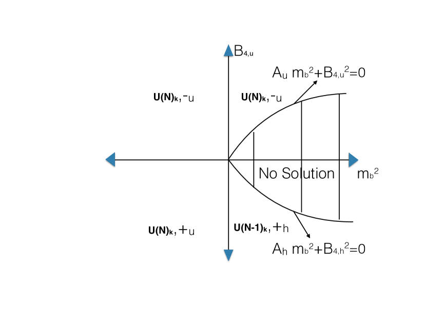
(a) Subdominant solutions

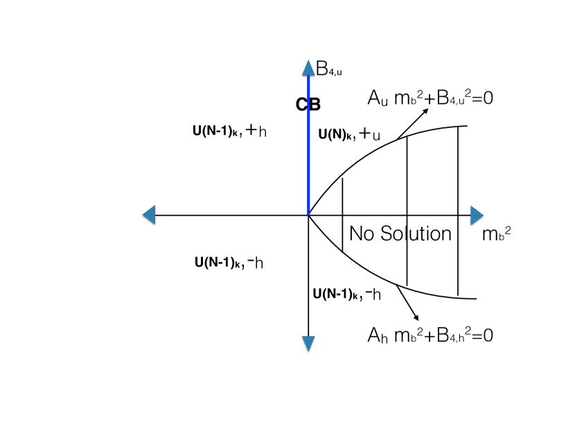
(b) Dominant solutions

Figure 22: Graphs of the domain of existence of the dominant and subdominant solutions to the gap equation for $\displaystyle x_{6}>\phi_{2}$. The dominant and subdominant solutions merge along the two parabolas in the graphs above. The solution space may thus be thought of as a double cover of the compliment of the unshaded portion of the $\displaystyle m_{b}^{2}$-$\displaystyle B_{4,u}$ plane.

The set of solutions to the gap equation in this case was described in section 4 and is schematically plotted in Figure 22. In this subsection we will demonstrate that the solutions depicted in Figure 22(b) are free-energetically dominant over those in Figure 22(a), and so represent the true phase diagram of the theory.

In order to analyze the free energies it is useful define the dimensionless parameter $\displaystyle\nu$ by

$$\nu\equiv\frac{m_{b}^{2}}{B_{4,u}^{2}}.$$ (358)

This definition is useful as it follows from dimensional analysis that the free energy in each phase – and hence the difference of free energies between any two phases – is given by $\displaystyle|B_{4,u}|^{3}$ times a function of the dimensionless parameter $\displaystyle\nu$. In other words, the phase structure of our theory depends on $\displaystyle B_{4,u}$ and $\displaystyle m_{b}^{2}$ only through the dimensionless combination $\displaystyle\nu$. Given any two phases $\displaystyle X$ and $\displaystyle Y$ with free energies $\displaystyle F_{X}$ and $\displaystyle F_{Y}$ let us define

$${\cal F}_{XY}\equiv\frac{F_{X}-F_{Y}}{|B_{4,u}|^{3}};$$ (359)

this depends only on $\displaystyle\nu$ (of course it also depends on $\displaystyle\lambda_{B}$ and $\displaystyle x_{6}$, and on the sign of $\displaystyle B_{4,u}$, but this dependence is suppressed in our notation).

For $\displaystyle B_{4,u}>0$ and $\displaystyle m_{b}^{2}>0$ a short computation reveals that

$${\cal F}_{-_{u}+_{u}}(\nu)=-4\frac{\lambda_{B}}{\lambda_{F}}\frac{\left(4+\nu(4-(4+3x_{6})\lambda_{B}^{2})\right)^{\frac{3}{2}}}{\left(4-(4+3x_{6})\lambda_{B}^{2}\right)^{2}}.$$ (360)

As $\displaystyle\frac{\lambda_{B}}{\lambda_{F}}<0$ it follows immediately that this quantity is positive, and so the phase $\displaystyle+_{u}$ is dominant.

For $\displaystyle B_{4,u}<0$ and $\displaystyle m_{b}^{2}>0$ a similar computation yields

$${\cal F}_{+_{h}-_{h}}(\nu)=-4\frac{\lambda_{B}}{\lambda_{F}}\frac{\left(4+\nu(4-(4+3x_{6})\lambda_{B}^{2})\right)^{\frac{3}{2}}}{\left(4-(4+3x_{6})\lambda_{B}^{2}\right)^{2}}.$$ (361)

Once again using the fact that $\displaystyle\frac{\lambda_{B}}{\lambda_{F}}<0$ it follows that $\displaystyle{\cal F}_{+_{h}-_{h}}(\nu)$ is positive, so that the phase $\displaystyle-_{h}$ is dominant.

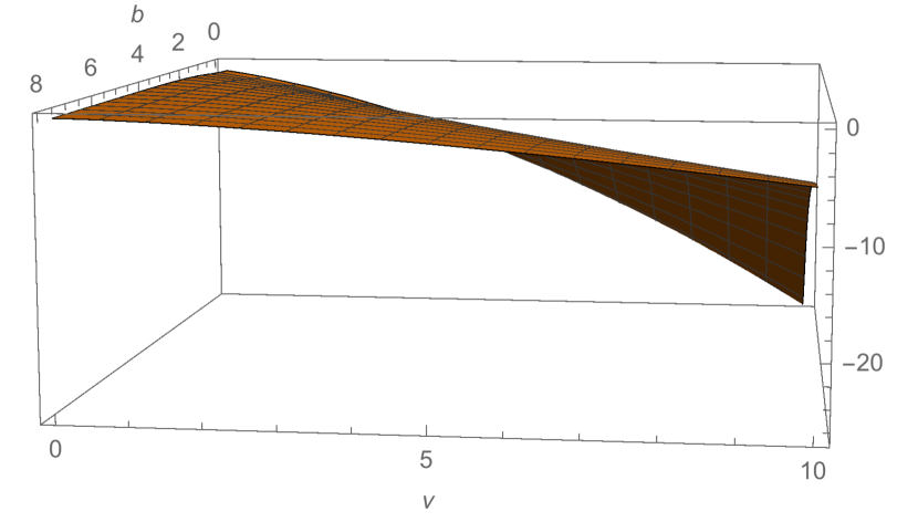
(a) A plot of $\displaystyle-{\cal F}_{-_{u}+_{h}}$ at $\displaystyle\lambda_{B}=\frac{1}{2}$, when $\displaystyle B_{4,u}>0$ and $\displaystyle m_{b}^{2}<0$. The axes of our plot are $\displaystyle\nu$ and $\displaystyle b$, where $\displaystyle b^{2}=x_{6}-\phi_{2}$. We see that everywhere $\displaystyle-{\cal F}_{-_{u}+_{h}}<0$, demonstrating that $\displaystyle+_{h}$ is the dominant phase.

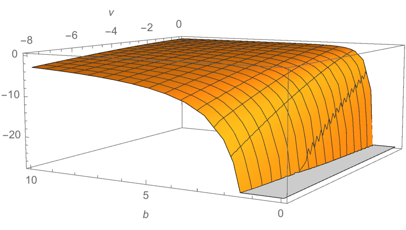
(b) A plot of $\displaystyle-{\cal F}_{+_{u}-_{h}}$ at $\displaystyle\lambda_{B}=\frac{1}{2}$, when $\displaystyle B_{4,u}<0$ and $\displaystyle m_{b}^{2}<0$. Once again the axes are $\displaystyle\nu$ and $\displaystyle b$, where $\displaystyle b$ was defined in the caption to the left. We see that $\displaystyle-{\cal F}_{+_{u}-_{h}}<0$, so that $\displaystyle-_{h}$ is the dominant phase.

Figure 23:

For $\displaystyle m_{b}^{2}<0$, the expressions for $\displaystyle{\cal F}_{-_{u}+_{h}}$ (when $\displaystyle B_{4,u}>0$) and for $\displaystyle{\cal F}_{+_{u}-_{h}}$ (when $\displaystyle B_{4,u}<0$) are messier. Rather than analytically massaging them into a manifestly positive definite form, we found it easier to simply plot them using Mathematica. Our plots are presented in Figure 23. The plots clearly reveal that both of these are positive for all $\displaystyle\nu$ and at all allowed values of $\displaystyle x_{6}$, at $\displaystyle\lambda_{B}=\frac{1}{2}$, consistent with our statements above (we have generated similar plots at various values of $\displaystyle\lambda_{B}$ and always find similar results).

F.2 $\displaystyle\phi_{1}<x_{6}<\phi_{2}$

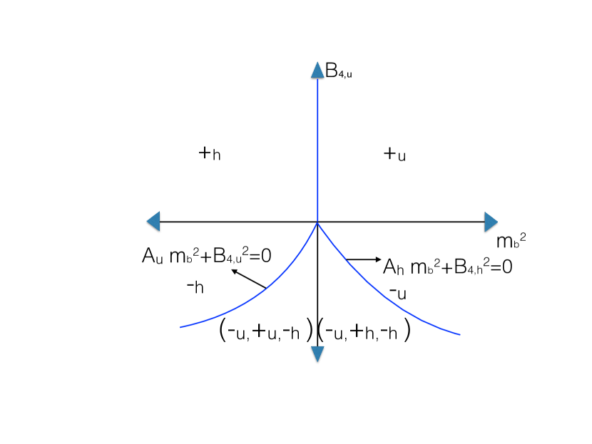
Figure 24: A graph of the domain of existence of solutions to the gap equation for $\displaystyle\phi_{2}>x_{6}>\phi_{1}$. We have a single solution outside the two parabolas, but three different solutions between these two parabolas. The $\displaystyle+_{u}$ and $\displaystyle-_{u}$ solutions reduce to each other on the left parabola while the $\displaystyle+_{h}$ and $\displaystyle-_{h}$ solutions reduce to each other on the right parabola. Moreover the $\displaystyle+_{u}$ and $\displaystyle+_{h}$ solutions continue into each other through a second order phase transition along the negative $\displaystyle B_{4,u}$ axis. It follows that the space of solutions represents a single cover of parameter space outside the two parabolas, but a triple cover of parameter space inside the two parabolas. Note that the $\displaystyle(+_{u},-_{u})$ and $\displaystyle(+_{h},-_{h})$ phases correspond to $\displaystyle U(N)_{\kappa}$ and $\displaystyle U(N-1)_{\kappa}$ theories, respectively.

Next we study the zero temperature phase diagram of our theory in the intermediate range $\displaystyle\phi_{1}<x_{6}<\phi_{2}$, as a function of $\displaystyle B_{4,u}$ and $\displaystyle m_{b}^{2}$. As noted in (201), in this range of parameters $\displaystyle A_{u}$ is positive while $\displaystyle A_{h}$ is negative. For most parameters here there is just a single solution to the gap equation, but for $\displaystyle B_{4,u}<0$ and in the region where $\displaystyle-B_{4,u}^{2}/A_{u}<m_{b}^{2}<-B_{4,h}^{2}/A_{h}$ there are three solutions, so we need to check which one dominates. The solutions are the $\displaystyle-_{h}$ and $\displaystyle-_{u}$ solutions, and in addition the $\displaystyle+_{u}$ solution for $\displaystyle m_{b}^{2}<0$, and the $\displaystyle+_{h}$ solution for $\displaystyle m_{b}^{2}>0$. All of this is summarized in Figure 24. We will now demonstrate that the $\displaystyle+$ solutions never dominate in this region, and that there is a first order phase transition somewhere in the middle of this region, between the $\displaystyle-_{u}$ and $\displaystyle-_{h}$ solutions.

In the region where three solutions exist and $\displaystyle m_{b}^{2}<0$ we find that

$${\cal F}_{-_{u}+_{u}}=4\frac{\lambda_{B}}{\lambda_{F}}\frac{\left(4+\nu(4-(4+3x_{6})\lambda_{B}^{2})\right)^{\frac{3}{2}}}{\left(4-(4+3x_{6})\lambda_{B}^{2}\right)^{2}}.$$ (362)

As the right-hand side of (362) is negative, it follows that $\displaystyle-_{u}$ always has a lower free energy than (and so is thermodynamically dominant compared to) $\displaystyle+_{u}$.

Similarly, for $\displaystyle m_{b}^{2}>0$ we find that

$$\begin{split}&{\cal F}_{-_{h}+_{h}}\\ &=-\frac{2\lambda_{B}^{2}}{(1-\alpha)^{2}(\lambda_{B}^{2}-{\hat{\lambda}}_{B}^{2})^{2}}\sqrt{\frac{{\hat{\lambda}}_{B}^{2}+(1-\alpha)\nu(\lambda_{B}^{2}-{\hat{\lambda}}_{B}^{2})}{\lambda_{B}^{2}}}\frac{{\hat{\lambda}}_{B}^{3}+(1-\alpha)\nu{\hat{\lambda}}_{B}\left(\lambda_{B}^{2}-{\hat{\lambda}}_{B}^{2}\right)}{\lambda_{F}}.\end{split}$$ (363)

The right-hand side of (363) is everywhere negative, establishing that the solutions $\displaystyle-_{h}$ are always thermodynamically preferred compared to $\displaystyle+_{h}$.

It follows that in the intersection region, the dominant phase is everywhere either $\displaystyle-_{u}$ (which clearly dominates also for $\displaystyle m_{b}^{2}>-B_{4,h}^{2}/A_{h}$ where it is the only solution) or $\displaystyle-_{h}$ (which clearly dominates also for $\displaystyle m_{b}^{2}<-B_{4,u}^{2}/A_{u}$). In order to see which phase dominates, we have plotted in Figure 25 $\displaystyle{\cal F}_{-_{h}-_{u}}$ as a function of $\displaystyle\nu$ and $\displaystyle\alpha$ at $\displaystyle\lambda_{B}=\frac{1}{2}$ (the analogous plots at different values of $\displaystyle\lambda_{B}$ are all similar), where $\displaystyle\alpha$ is defined by the relation

$$x_{6}=\alpha\phi_{1}+(1-\alpha)\phi_{2},$$ (364)

so that it goes between zero and one as we increase $\displaystyle x_{6}$.

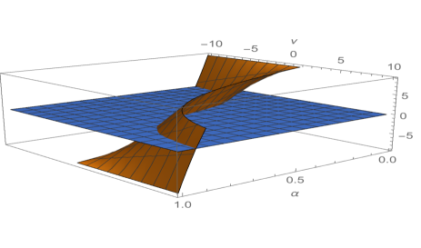
Figure 25: $\displaystyle{\cal F}_{-_{h}-_{u}}$ in the $\displaystyle\alpha$ and $\displaystyle\nu$ plane at $\displaystyle\lambda_{B}=\frac{1}{2}$. The plane with blue color is to indicate when $\displaystyle{\cal F}_{-_{h}-_{u}}$ is positive or negative.

We see that for every value of $\displaystyle\alpha$ there is a phase transition as we change $\displaystyle\nu$ (or $\displaystyle m_{b}^{2}$). We see that the phase $\displaystyle-_{u}$ is thermodynamically dominant for $\displaystyle\nu\leq\nu_{c}$, while $\displaystyle-_{h}$ is dominant for $\displaystyle\nu\geq\nu_{c}$, where the quantity $\displaystyle\nu_{c}(\alpha)$ is plotted for $\displaystyle\lambda_{B}=\frac{1}{2}$ in Figure 26.

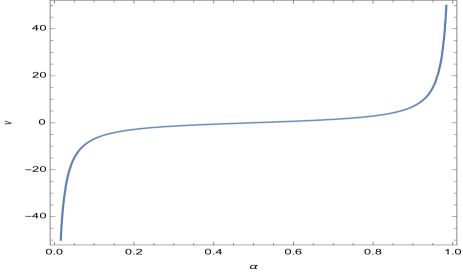
Figure 26: $\displaystyle\nu_{c}$ as a function of $\displaystyle\alpha$ at $\displaystyle\lambda_{B}=\frac{1}{2}.$

Note that $\displaystyle\nu_{c}\to-\infty$ as $\displaystyle\alpha\to 0$ (i.e. as $\displaystyle x_{6}\to\phi_{2}$). On the other hand $\displaystyle\nu_{c}\to+\infty$ as $\displaystyle\alpha\to 1$. The resulting phase diagram is drawn in Figure 7 in Section 4.

F.3 $\displaystyle x_{6}<\phi_{1}$

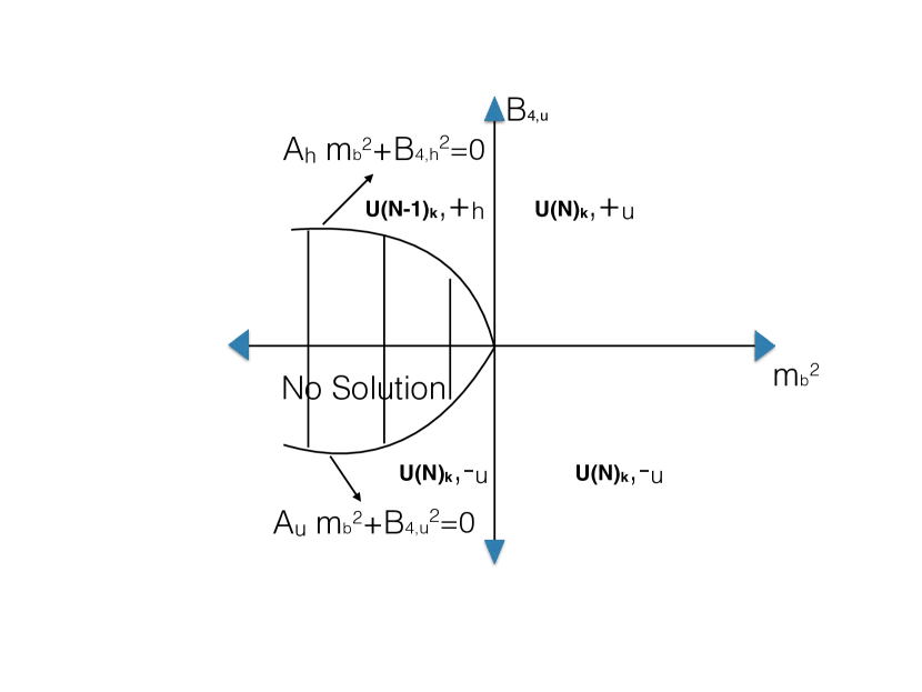
(a) Dominant Solutions

(b) Subdominant Solutions

Figure 27: Graphs of the domain of existence of the dominant and subdominant solutions to the gap equation for $\displaystyle x_{6}<\phi_{1}$. The dominant and subdominant solutions merge along the two parabolas in the graphs above. The solution space may thus be thought of as a double cover of the compliment of the unshaded portion of the $\displaystyle m_{b}^{2}$-$\displaystyle B_{4,u}$ plane.

The situation in this range of parameters is very similar to that of $\displaystyle x_{6}>\phi_{2}$, with two solutions or none in all regions of the parameter space (see Figure 27). For $\displaystyle B_{4,u}>0$ the $\displaystyle+_{u}$ or $\displaystyle+_{h}$ phase dominates, with a second order phase transition between them at $\displaystyle m_{b}^{2}=0$, while for $\displaystyle B_{4,u}<0$ the $\displaystyle-_{u}$ phase dominates.

When $\displaystyle B_{4,u}<0$ and $\displaystyle m_{b}^{2}<0$ we have

$${\cal F}_{-_{u}+_{u}}=4\frac{\lambda_{B}}{\lambda_{F}}\frac{\left(4+\nu(4-(4+3x_{6})\lambda_{B}^{2})\right)^{\frac{3}{2}}}{\left(4-(4+3x_{6})\lambda_{B}^{2}\right)^{2}}.$$ (365)

The right-hand side of (365) is always negative, establishing that $\displaystyle-_{u}$ is the dominant phase.

In a similar manner, for $\displaystyle B_{4,u}>0$ and $\displaystyle m_{b}^{2}<0$ we find

$${\cal F}_{+_{h}-_{h}}=-4\frac{{\hat{\lambda}}_{B}}{\lambda_{F}}\frac{\left(4\frac{{\hat{\lambda}}_{B}^{2}}{\lambda_{B}^{2}}+\nu(-4+(4+3x_{6}){\hat{\lambda}}_{B}^{2})\right)^{\frac{3}{2}}}{\left(4-(4+3x_{6}){\hat{\lambda}}_{B}^{2}\right)^{2}}$$ (366)

which is again negative, establishing the thermodynamical dominance of $\displaystyle+_{h}$ over $\displaystyle-_{h}$.

For $\displaystyle m_{b}^{2}>0$ we do not have analytic expressions. We present a numerical evaluation of the free energy differences in Figure 28, for the particular value $\displaystyle\lambda_{B}=\frac{1}{2}$ (these graphs are qualitatively similar at all values of $\displaystyle\lambda_{B}$). It justifies the phase structure described above.

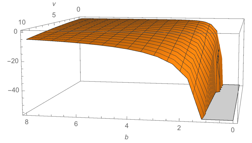
(a) A plot of $\displaystyle{\cal F}_{+_{u}-_{h}}$ for $\displaystyle B_{4,u}>0$, $\displaystyle m_{b}^{2}>0$. The axes are $\displaystyle\nu$ and $\displaystyle b$ where $\displaystyle x_{6}=\phi_{1}-b^{2}$. Note that $\displaystyle{\cal F}_{+_{u}-_{h}}$ is everywhere negative.

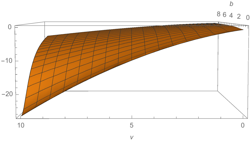
(b) A plot of $\displaystyle{\cal F}_{-_{u}+_{h}}$ for $\displaystyle B_{4,u}<0$, $\displaystyle m_{b}^{2}>0$, with the same axes. Note that $\displaystyle{\cal F}_{-_{u}+_{h}}$ is everywhere negative.

Figure 28:

References

- (1) I. R. Klebanov and A. M. Polyakov, AdS dual of the critical O(N) vector model, Phys. Lett. B550 (2002) 213–219, [hep-th/0210114].
- (2) E. Sezgin and P. Sundell, Massless higher spins and holography, Nucl. Phys. B644 (2002) 303–370, [hep-th/0205131].
- (3) S. Giombi and X. Yin, Higher Spin Gauge Theory and Holography: The Three-Point Functions, JHEP 09 (2010) 115, [0912.3462].
- (4) S. Giombi, S. Minwalla, S. Prakash, S. P. Trivedi, S. R. Wadia and X. Yin, Chern-Simons Theory with Vector Fermion Matter, Eur. Phys. J. C72 (2012) 2112, [1110.4386].
- (5) C.-M. Chang, S. Minwalla, T. Sharma and X. Yin, ABJ Triality: from Higher Spin Fields to Strings, J. Phys. A46 (2013) 214009, [1207.4485].
- (6) S. Giombi, Higher Spin-CFT Duality, in Proceedings, Theoretical Advanced Study Institute in Elementary Particle Physics: New Frontiers in Fields and Strings (TASI 2015): Boulder, CO, USA, June 1-26, 2015, pp. 137–214, 2017, 1607.02967, DOI.
- (7) O. Aharony, O. Bergman, D. L. Jafferis and J. Maldacena, N=6 superconformal Chern-Simons-matter theories, M2-branes and their gravity duals, JHEP 10 (2008) 091, [0806.1218].
- (8) J. Maldacena and A. Zhiboedov, Constraining Conformal Field Theories with A Higher Spin Symmetry, J.Phys. A46 (2013) 214011, [1112.1016].
- (9) J. Maldacena and A. Zhiboedov, Constraining conformal field theories with a slightly broken higher spin symmetry, Class.Quant.Grav. 30 (2013) 104003, [1204.3882].
- (10) D. Gaiotto and X. Yin, Notes on superconformal Chern-Simons-Matter theories, JHEP 08 (2007) 056, [0704.3740].
- (11) F. Benini, C. Closset and S. Cremonesi, Comments on 3d Seiberg-like dualities, JHEP 1110 (2011) 075, [1108.5373].
- (12) J. Park and K.-J. Park, Seiberg-like Dualities for 3d N=2 Theories with SU(N) gauge group, JHEP 10 (2013) 198, [1305.6280].
- (13) O. Aharony, S. S. Razamat, N. Seiberg and B. Willett, 3d dualities from 4d dualities, JHEP 07 (2013) 149, [1305.3924].
- (14) A. Giveon and D. Kutasov, Seiberg Duality in Chern-Simons Theory, Nucl.Phys. B812 (2009) 1–11, [0808.0360].
- (15) S. Jain, S. Minwalla and S. Yokoyama, Chern Simons duality with a fundamental boson and fermion, JHEP 1311 (2013) 037, [1305.7235].
- (16) K. Inbasekar, S. Jain, S. Mazumdar, S. Minwalla, V. Umesh and S. Yokoyama, Unitarity, crossing symmetry and duality in the scattering of susy matter Chern-Simons theories, JHEP 10 (2015) 176, [1505.06571].
- (17) G. Gur-Ari and R. Yacoby, Three Dimensional Bosonization From Supersymmetry, 1507.04378.
- (18) A. Kapustin, B. Willett and I. Yaakov, Tests of Seiberg-like Duality in Three Dimensions, 1012.4021.
- (19) B. Willett and I. Yaakov, N=2 Dualities and Z Extremization in Three Dimensions, 1104.0487.
- (20) A. Kapustin, Seiberg-like duality in three dimensions for orthogonal gauge groups, 1104.0466.
- (21) K. Intriligator and N. Seiberg, Aspects of 3d N=2 Chern-Simons-Matter Theories, JHEP 07 (2013) 079, [1305.1633].
- (22) O. Aharony, G. Gur-Ari and R. Yacoby, d=3 Bosonic Vector Models Coupled to Chern-Simons Gauge Theories, JHEP 1203 (2012) 037, [1110.4382].
- (23) D. Gaiotto, Z. Komargodski and N. Seiberg, Time-Reversal Breaking in QCD4, Walls, and Dualities in 2+1 Dimensions, 1708.06806.
- (24) J. Gomis, Z. Komargodski and N. Seiberg, Phases Of Adjoint QCD3 And Dualities, 1710.03258.
- (25) D. Radicevic, Disorder Operators in Chern-Simons-Fermion Theories, JHEP 03 (2016) 131, [1511.01902].
- (26) O. Aharony, Baryons, monopoles and dualities in Chern-Simons-matter theories, JHEP 02 (2016) 093, [1512.00161].
- (27) O. Aharony, G. Gur-Ari and R. Yacoby, Correlation Functions of Large N Chern-Simons-Matter Theories and Bosonization in Three Dimensions, JHEP 1212 (2012) 028, [1207.4593].
- (28) N. Seiberg, T. Senthil, C. Wang and E. Witten, A Duality Web in 2+1 Dimensions and Condensed Matter Physics, 1606.01989.
- (29) G. Gur-Ari and R. Yacoby, Correlators of Large N Fermionic Chern-Simons Vector Models, JHEP 1302 (2013) 150, [1211.1866].
- (30) A. Bedhotiya and S. Prakash, A test of bosonization at the level of four-point functions in Chern-Simons vector models, JHEP 12 (2015) 032, [1506.05412].
- (31) S. Jain, M. Mandlik, S. Minwalla, T. Takimi, S. R. Wadia and S. Yokoyama, Unitarity, Crossing Symmetry and Duality of the S-matrix in large N Chern-Simons theories with fundamental matter, JHEP 04 (2015) 129, [1404.6373].
- (32) Y. Dandekar, M. Mandlik and S. Minwalla, Poles in the -Matrix of Relativistic Chern-Simons Matter theories from Quantum Mechanics, JHEP 04 (2015) 102, [1407.1322].
- (33) S. Yokoyama, Scattering Amplitude and Bosonization Duality in General Chern-Simons Vector Models, 1604.01897.
- (34) S. Jain, S. P. Trivedi, S. R. Wadia and S. Yokoyama, Supersymmetric Chern-Simons Theories with Vector Matter, JHEP 1210 (2012) 194, [1207.4750].
- (35) O. Aharony, S. Giombi, G. Gur-Ari, J. Maldacena and R. Yacoby, The Thermal Free Energy in Large N Chern-Simons-Matter Theories, JHEP 1303 (2013) 121, [1211.4843].
- (36) S. Jain, S. Minwalla, T. Sharma, T. Takimi, S. R. Wadia et al., Phases of large vector Chern-Simons theories on , JHEP 1309 (2013) 009, [1301.6169].
- (37) T. Takimi, Duality and higher temperature phases of large N Chern-Simons matter theories on x , JHEP 1307 (2013) 177, [1304.3725].
- (38) S. Yokoyama, A Note on Large N Thermal Free Energy in Supersymmetric Chern-Simons Vector Models, JHEP 1401 (2014) 148, [1310.0902].
- (39) S. Yokoyama, Chern-Simons-Fermion Vector Model with Chemical Potential, JHEP 1301 (2013) 052, [1210.4109].
- (40) A. Karch and D. Tong, Particle-Vortex Duality from 3d Bosonization, Phys. Rev. X6 (2016) 031043, [1606.01893].
- (41) R. D. Pisarski, Fixed point structure of in three-dimensions at large N, Phys. Rev. Lett. 48 (1982) 574–576.
- (42) E. Pomoni and L. Rastelli, Large N Field Theory and AdS Tachyons, JHEP 04 (2009) 020, [0805.2261].
- (43) R. Yacoby, Scalar Correlators in Bosonic Chern-Simons Vector Models, 1805.11627.
- (44) S. Minwalla and S. Yokoyama, Chern Simons Bosonization along RG Flows, JHEP 02 (2016) 103, [1507.04546].
- (45) A. Dey, I. Halder, S. Jain, L. Janagal, S. Minwalla and N. Prabhakar, Regular Boson Critical Fermion Chern-Simons dualities in the Higgsed Phase, To appear, .
- (46) P.-S. Hsin and N. Seiberg, Level/rank Duality and Chern-Simons-Matter Theories, JHEP 09 (2016) 095, [1607.07457].
- (47) W. Siegel, Supersymmetric Dimensional Regularization via Dimensional Reduction, Phys. Lett. 84B (1979) 193–196.
- (48) A. N. Vasiliev, Yu. M. Pismak and Yu. R. Khonkonen, 1/N Expansion: Calculation of the exponent in the order by the conformal bootstrap method, Theor. Math. Phys. 50 (1982) 127–134.
- (49) A. Bzowski, P. McFadden and K. Skenderis, Implications of conformal invariance in momentum space, JHEP 03 (2014) 111, [1304.7760].
- (50) G. J. Turiaci and A. Zhiboedov, Veneziano Amplitude of Vasiliev Theory, 1802.04390.
- (51) O. Aharony, L. F. Alday, A. Bissi and R. Yacoby, The Analytic Bootstrap for Large Chern-Simons Vector Models, 1805.04377.
- (52) S. Giombi, V. Gurucharan, V. Kirilin, S. Prakash and E. Skvortsov, On the Higher-Spin Spectrum in Large N Chern-Simons Vector Models, JHEP 01 (2017) 058, [1610.08472].
- (53) O. Aharony, F. Benini, P.-S. Hsin and N. Seiberg, Chern-Simons-matter dualities with and gauge groups, JHEP 02 (2017) 072, [1611.07874].
- (54) S. Choudhury, A. Dey, I. Halder, S. Jain, L. Janagal, S. Minwalla et al., Bose-Fermi Chern-Simons Dualities in the Higgsed Phase, 1804.08635.
- (55) S. Giombi, V. Kirilin and E. Skvortsov, Notes on Spinning Operators in Fermionic CFT, 1701.06997.
- (56) L. V. Avdeev, D. I. Kazakov and I. N. Kondrashuk, Renormalizations in supersymmetric and nonsupersymmetric nonAbelian Chern-Simons field theories with matter, Nucl. Phys. B391 (1993) 333–357.
- (57) F. Benini, Three-dimensional dualities with bosons and fermions, JHEP 02 (2018) 068, [1712.00020].
- (58) K. Jensen, A master bosonization duality, JHEP 01 (2018) 031, [1712.04933].
- (59) E. Witten, Multitrace operators, boundary conditions, and AdS / CFT correspondence, hep-th/0112258.
- (60) S. Grozdanov, Wilsonian Renormalisation and the Exact Cut-Off Scale from Holographic Duality, JHEP 06 (2012) 079, [1112.3356].
- (61) D. Das, S. R. Das and G. Mandal, Double Trace Flows and Holographic RG in dS/CFT correspondence, JHEP 11 (2013) 186, [1306.0336].
- (62) O. Aharony, G. Gur-Ari and N. Klinghoffer, The Holographic Dictionary for Beta Functions of Multi-trace Coupling Constants, JHEP 05 (2015) 031, [1501.06664].
- (63) A. Kapustin and B. Willett, Wilson loops in supersymmetric Chern-Simons-matter theories and duality, 1302.2164.
- (64) O. Aharony and D. Fleischer, IR Dualities in General 3d Supersymmetric SU(N) QCD Theories, JHEP 02 (2015) 162, [1411.5475].
- (65) S. G. Naculich, H. A. Riggs and H. J. Schnitzer, Group Level Duality in WZW Models and Chern-Simons Theory, Phys. Lett. B246 (1990) 417–422.
- (66) M. Camperi, F. Levstein and G. Zemba, The Large Limit of Chern-Simons Gauge Theory, Phys. Lett. B247 (1990) 549–554.
- (67) T. Nakanishi and A. Tsuchiya, Level rank duality of WZW models in conformal field theory, Commun. Math. Phys. 144 (1992) 351–372.
- (68) S. G. Naculich and H. J. Schnitzer, Level-rank duality of the U(N) WZW model, Chern-Simons theory, and 2-D qYM theory, JHEP 06 (2007) 023, [hep-th/0703089].