Nonlinear optics of graphene and other 2D materials in layered structures

Abstract

We present a theoretical framework for nonlinear optics of graphene and other 2D materials in layered structures. We derive a key equation to find the effective electric field and the sheet current density in the 2D material for given incident light beams. Our approach takes into account the effect of the surrounding environment and characterizes its contribution as a structure factor. We apply our approach to two experimental setups, and discuss the structure factors for several nonlinear optical processes including second harmonic generation, third harmonic generation, and parametric frequency conversion. Our systematic study gives a strict extraction method for the nonlinear coefficients, and provides new insights in how layered structures influence the nonlinear signal observed from 2D materials.

I Introduction

Graphene possesses extraordinary optical properties Bonaccorso et al. (2010), including broadband absorption Nair et al. (2008), the existence of tightly confined plasmon modes Low and Avouris (2014); Garcǐa de Abajo (2014); Ooi and Tan (2017), and extremely strong optical nonlinearities Glazov and Ganichev (2014); Sun et al. (2016); Autere et al. (2018). Most of these properties strongly depend on the chemical potential, which can be controlled chemically Pinto et al. (2009); Liu et al. (2011a), optically Ni et al. (2016), or with the use of an external gate voltage Novoselov et al. (2004). Since the first experimental demonstration of strong parametric frequency conversion (PFC) in graphene Hendry et al. (2010), much attention has been paid to its optical nonlinearities. With the integration of graphene onto photonic chips becoming a mature technology Bonaccorso et al. (2010); Xia et al. (2014); Vermeulen et al. (2016a), graphene is recognized as a potential resource for many photonic devices that exploit optical nonlinearities, including saturable absorbers Bao et al. (2009), broadband optical modulators Liu et al. (2011b, 2012); Ooi et al. (2014), optical switches Ooi et al. (2016), and wavelength converters Vermeulen et al. (2016a). For these applications to be developed, a full understanding of the nonlinear radiation of graphene is necessary. In general, this is determined by both the intrinsic optical nonlinearity of graphene, and the effects of the surrounding environment. Neither is sufficiently understood at this point.

The intrinsic optical nonlinearity of graphene has been studied extensively. Various experiments with graphene in free-space configurations, on waveguides, and on photonic crystals have been performed to investigate different nonlinear phenomena, including PFC Hendry et al. (2010); Jiang et al. (2018), third harmonic generation (THG) Kumar et al. (2013); Hong et al. (2013); Säynätjoki et al. (2013); Jiang et al. (2018); Soavi et al. (2018), second harmonic generation (SHG) Dean and van Driel (2009, 2010); Bykov et al. (2012); An et al. (2013, 2014); Lin et al. (2014), Kerr effects (or self-phase modulation, SPM) and two photon absorption Xing et al. (2010); Wu et al. (2011); Yang et al. (2011); Zhang et al. (2012); Gu et al. (2012); Vermeulen et al. (2016b); Dremetsika et al. (2016); Vermeulen et al. (2018), and coherent current injection Sun et al. (2010, 2012). The extracted effective bulk third order susceptibilities $\chi_{\text{eff}}^{(3)}$ are in the range of $10^{-13}-10^{-19}\text{~{}m}^{2}/\text{V}^{2}$, while the values of the effective bulk second order susceptibilities $\chi_{\text{eff}}^{(2)}$ are seldom extracted. Recent experiments have shown the unusual negative sign of graphene’s nonlinear refractive index Vermeulen et al. (2016b); Dremetsika et al. (2016); Demetriou et al. (2016), the ability to tune the nonlinearity by varying the chemical potential Jiang et al. (2018); Soavi et al. (2018), and the possibility of having quasi-exponentially growing SPM in graphene on waveguides Vermeulen et al. (2018). Most of the existing microscopic theories Cheng et al. (2014); *Corrigendum_NewJ.Phys._18_29501_2016_Cheng; Cheng et al. (2015a); *Phys.Rev.B_93_39904_2016_Cheng; Cheng et al. (2015b); Soh et al. (2016); Rostami and Polini (2016); Mikhailov (2016); Wang et al. (2016); Cheng et al. (2017); Mikhailov (2017); Marini et al. (2017); Rostami et al. (2017); Avetissian and Mkrtchian (2018) focus on the dependence of the sheet conductivities $\sigma^{(n)}$ ($\propto-i\omega\chi^{(n)}_{\text{eff}}$) on incident light frequencies, temperature, and doping levels. When scattering is described within a phenomenological relaxation time approximation, the calculated $\chi^{(3)}_{\text{eff}}$ are about two orders of magnitude smaller than most values extracted from earlier experiments for lightly doped graphene Cheng et al. (2014); *Corrigendum_NewJ.Phys._18_29501_2016_Cheng; Cheng et al. (2015a); *Phys.Rev.B_93_39904_2016_Cheng; Soh et al. (2016). Several effects have been considered that might bring theory in better agreement with these experiments, including saturation of the optical nonlinearity Cheng et al. (2015b); Marini et al. (2017), the influence of cascaded second order processes Constant et al. (2015); Rostami et al. (2017), and novel plasmonic effects Cox and Javier García de Abajo (2014); Rostami et al. (2017), but none of them can sufficiently enhance the calculated conductivities. Recent experiment on light propagating in graphene-covered waveguides Vermeulen et al. (2018) has shown that free-carrier refraction plays an important role, and that a treatment beyond perturbation theory is required there. This may be necessary in other excitation configurations as well. However, agreement with perturbative calculations is satisfactory in recent free-space experiments, where the doping level of graphene is tuned over a large range Jiang et al. (2018); Soavi et al. (2018).

Besides the insufficient understanding of the physical mechanism for the intrinsic optical nonlinearity, the accurate extraction of the effective susceptibility itself from experimental data is also an outstanding problem, especially considering the one-atom thickness. Experimentally, two methods are widely used, both treating graphene as a thin film Hendry et al. (2010) with an effective thickness $d_{\text{gr}}\approx 3.3$ Å. One is simply to compare the radiation signal to a film with known susceptibility, and the other is to utilize the well-known results for a thin bulk sample in the limit of an undepleted fundamental Kumar et al. (2013); Boyd (2008). Neither strategy is based on a strict derivation of the response of a monolayer sample, and the effective susceptibility extracted from either method depends on the artificial thickness assigned to the graphene layer. For usual bulk materials, the generated nonlinear radiation can be worked out using coupled-mode theory Boyd (2008), in which a coherence length associated with the phase-matching condition arises in the derivation of the equations for the propagating fields. It has been pointed out that for weakly coupled 2D layers the atomic spacing between the layers should guarantee coherent radiation from the layers Autere et al. (2018); Zhao et al. (2016). Despite many investigations using standard software Kumar et al. (2013); Vincenti et al. (2013, 2014), and nonlinear boundary conditions Savostianova and Mikhailov (2015, 2017); Gorbach and Ivanov (2016); Gorbach (2013), there is still no systematic treatment of the response of graphene, taking into account its 2D nature, which could later be generalized to treat multilayer samples.

In this work we focus on how the surrounding environment affects the nonlinear radiation of general 2D materials inside layered structures. We model the current density in graphene as a “current sheet” described by a Dirac $\delta$-function, and derive a key equation for graphene nonlinear optics, from which the effective electric fields and current density inside 2D materials can be determined as a response to incident laser beams. These results are easily combined with the transfer matrix formalism, and are used to analyze the nonlinear fields generated by a graphene sheet on multilayered structures. The output fields $E_{\text{out}}$ are connected to incident fields $E_{\text{in}}$ in a form $E_{\text{out}}\propto{\sigma}^{(n)}\beta^{(n)}E_{\text{in}}^{n}$, with the structure factor $\beta^{(n)}$ describing the environmental effects. In certain structures, the contribution from the structure factor can be extremely large, providing a controllable way to enhance the generated nonlinear signals Vincenti et al. (2013, 2014); Yao et al. (2014); Constant et al. (2015); Tao et al. (2015). The equations we establish can be readily applied to the entire family of 2D materials, including bi-layer graphene, functionalized graphene, monolayer transition-metal dichalcogenides, black phosphorene, silicene, stanene, and so on. We also discuss whether or not a cascaded second order response can modify extracted effective third order nonlinear response coefficients.

We organize this paper as follows: In Sec. II we work out the equations for a suspended 2D layer, and obtain a consistent set of equations for the second and third order nonlinear response; in Sec. III we extend these results to a system with 2D materials embedded inside a multilayered structure; in Sec. IV we apply these results to a graphene-covered multilayered structure. We conclude in Sec. V.

II Suspended 2D layer

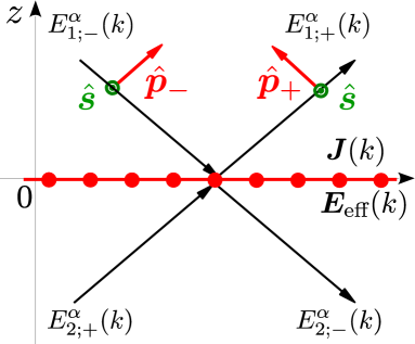
Figure 1: (color online) A suspended 2D layer at position $z=0$. Here $E_{j;\lambda}^{\alpha}(k)$ are the amplitudes of the $\alpha$-polarized components of the electric field propagating (or evanescent) in the $j$th region in the $\lambda$ direction; $\hat{\bm{s}}$ and $\hat{\bm{p}}_{\pm}$ are polarization vectors, with a compact notation $k=(\bm{\kappa},\omega)$. The sketch of the polarization vectors and the propagation directions is schematic, since in general $\hat{\bm{p}}_{\pm}$can have complex Cartesian components and the fields can be evanescent (See Appendix A). The 2D layer experiences an electric field $\bm{E}_{\text{eff}}(k)$ and possesses a sheet current $\bm{J}(k)$.

We first consider the optics of a suspended monolayer (or nearly-monolayer) structure, which is centered at $z=0$, as shown in Fig. 1. In the neighborhood of the monolayer the microscopic electric field and current density have a very complicated spatial dependence, with variations on an atomic scale, and their full description requires a very careful treatment Cheng et al. . However, for the calculation of radiation at optical frequencies with wavelengths much larger than these dimensions, a “$\delta$-model” for the current density can be introduced,

$$\bm{J}(z;k)=\delta(z)\bm{J}(k)\,,$$ (1)

where $k=(\bm{\kappa},\omega)$ indicates the in-plane wave vector $\bm{\kappa}$ and frequency $\omega$; for details of the notation see Appendix A. Here $\bm{J}(k)$ is a sheet current density. We will see that it mostly appears in the form

$$\vec{{\cal J}}(k)=\frac{\bm{J}(k)}{2c\epsilon_{0}}\,,$$ (2)

which has the dimension of an electric field.

Within this $\delta$-model all of space is split into three regions, $z>0$, $z=0$, and $z<0$, and both the regions $z>0$ and $z<0$ are vacuum. The electric field in the latter two regions are described by amplitudes $E_{j;\lambda}^{\alpha}(k)$, where $j=1,2$ is an index identifying the region ($z>0$ and $z<0$ respectively), $\lambda=+$ ($-$) stands for the upward (downward) propagating or evanescent direction, and $\alpha=s$ ($p$) identifies the $s$ ($p$)-polarized component. Using a Green function strategy Sipe (1987) (see Appendix B), we can connect the fields in the 1st and 2nd regions by

$$E_{1;+}^{\alpha}(k) = E_{2;+}^{\alpha}(k)+{\cal F}_{+}^{\alpha}(k)\,,$$ (3)

$$E_{2;-}^{\alpha}(k) = E_{1;-}^{\alpha}(k)+{\cal F}_{-}^{\alpha}(k)\,,$$ (4)

with

$${\cal F}_{\lambda}^{\alpha}(k)=-\frac{\widetilde{\omega}}{w_{0}(k)}\vec{{\cal J}}(k)\cdot\hat{\bm{e}}_{0;\lambda}^{\alpha}(k)\,.$$ (5)

The vectors $\hat{\bm{e}}_{0;\lambda}^{\alpha}(k)$ are the polarization vectors for the indicated polarizations $\alpha$ and propagation (or evanescent) directions $\lambda$, which are defined in Appendix A; $\widetilde{\omega}\equiv\omega/c$ and $w_{0}(k)=\sqrt{\widetilde{\omega}^{2}-\kappa^{2}}$. The fields in Eqs. (3) and (4) include any incident fields that are present, from sources or media above (amplitude $E_{1;-}^{\alpha}(k)$) or below (amplitude $E_{2;+}^{\alpha}(k)$) the monolayer.

To determine $\vec{{\cal J}}(k)$ and thus find the total fields above and below the monolayer one needs to specify the response of the medium to the full field, including that from the monolayer itself. Dealing with the $\boldsymbol{\hat{z}}$ component of the response is here particularly difficult, because the $\boldsymbol{\hat{z}}$ component of the field would vary strongly over that microscopic thickness. Largely this strongly varying field would be included in a standard calculation of the response as done in condensed matter physics, and thus would be included in such a calculation of the linear or nonlinear response coefficients; we need to identify an effective driving field $\bm{E}_{\text{eff}}(k)$ that would lead to a calculation of these response coefficients. We follow the standard approach (see, e.g. Gorbach and Ivanov (2016)) and take $\bm{E}_{\text{eff}}(k)$ to be the average of the fields above and below the 2D layer,

$$\bm{E}_{\text{eff}}(k)=\frac{1}{2}\sum_{\lambda\alpha}[E_{1;\lambda}^{\alpha}(k)+E_{2;\lambda}^{\alpha}(k)]\hat{\bm{e}}_{0;\lambda}^{\alpha}(k)\,.$$ (6)

The task of determining the dependence of $\vec{{\cal J}}(k)$ on $\bm{E}_{\text{eff}}$(k) is then assigned to condensed matter physics; it has been widely studied both perturbatively Cheng et al. (2014); *Corrigendum_NewJ.Phys._18_29501_2016_Cheng; Cheng et al. (2015a); *Phys.Rev.B_93_39904_2016_Cheng; Mikhailov (2016); Rostami and Polini (2016); Rostami et al. (2017) and numerically Cheng et al. (2015b); Avetissian and Mkrtchian (2018). Other strategies and their associated definitions of $\bm{E}_{\text{eff}}(k)$ could be considered, but would just shift how much of the problem was relegated to the task of determining $\vec{{\cal J}}[k;\bm{E}_{\text{eff}}(k)],$ and how much was relegated to the task of constructing $\bm{E}_{\text{eff}}(k)$ from the incident field and the field from the microscopic current density itself. The advantage of the use of Eq. (6) is that it is a simple expression but still completely contains the radiation reaction field due to the current sheet, so that the effect of $\bm{E}_{\text{eff}}(k)$ on the sheet includes the consequences of its radiation carrying energy away; energy conservation is thus respected.

II.1 Effective fields and sheet current density inside the 2D layer

Once the functional $\vec{{\cal J}}[k;\bm{E}_{\text{eff}}]$ is known, Eqs. (3), (4), and (6) are closed. Substituting Eqs. (3) and (4) into Eq. (6) we express the effective fields from $\vec{{\cal J}}(k)$ as

$$\bm{E}_{\text{eff}}(k)=\bm{E}_{\text{2D}}^{0}(k)+{\cal Q}^{0}(k)\vec{{\cal J}}(k)\,.$$ (7)

Here $\bm{E}_{\text{2D}}^{0}(k)=\sum_{\alpha}E_{1;-}^{\alpha}(k)\hat{\bm{e}}_{0;-}^{\alpha}(k)+\sum_{\alpha}E_{2;+}^{\alpha}(k)\hat{\bm{e}}_{0;+}^{\alpha}(k)$ is the incident field at the 2D layer (the field without the presence of the 2D layer), and ${\cal Q}^{0}(k)=-\frac{\widetilde{\omega}}{w_{0}}\hat{\bm{s}}(k)\hat{\bm{s}}(k)-\frac{w_{0}}{\widetilde{\omega}}\hat{\bm{\kappa}}\hat{\bm{\kappa}}-\frac{\kappa^{2}}{w_{0}\widetilde{\omega}}\hat{\bm{z}}\hat{\bm{z}}$ is a radiation coefficient tensor matrix associated with the 2D layer. The second term at the right hand side of Eq. (7) gives the onsite fields induced by the sheet current. Equation (7) is our key result; what is also needed to solve for the radiated fields is the identification of the functional $\vec{{\cal J}}[k;\bm{E}_{\text{eff}}]$ from a response theory in condensed matter physics. Using $\vec{{\cal J}}[k;\bm{E}_{\text{eff}}]$ together with Eq. (7) then leads to a self-consistent solution for the fields and the sheet current.

For weak electric fields, the sheet current density can be written into a power expansion of the effective fields. Up to the third order terms, it is

$$\vec{{\cal J}}(k) = \eta^{(1)}(k)\bm{E}_{\text{eff}}(k)+\vec{{\cal J}}_{\text{nl}}(k)\,,$$ (8)

$$\vec{{\cal J}}_{\text{nl}}(k) = \int\frac{dk_{1}}{(2\pi)^{3}}\eta^{(2)}(k_{1},k-k_{1})\bm{E}_{\text{eff}}(k_{1})\bm{E}_{\text{eff}}(k-k_{1})$$ (9)

$$+\int\frac{dk_{1}dk_{2}}{(2\pi)^{6}}\eta^{(3)}(k_{1},k_{2},k-k_{1}-k_{2})$$

$$\quad\times\bm{E}_{\text{eff}}(k_{1})\bm{E}_{\text{eff}}(k_{2})\bm{E}_{\text{eff}}(k-k_{1}-k_{2})\,.$$

Here the tensors $\eta^{(1)}(k)=\sigma^{(1)}(k)/(2c\epsilon_{0})$, $\eta^{(2)}(k_{1},k_{2})=\sigma^{(2)}(k_{1},k_{2})/(2c\epsilon_{0})$, and $\eta^{(3)}(k_{1},k_{2},k_{3})=\sigma^{(3)}(k_{1},k_{2},k_{3})/(2c\epsilon_{0})$ are associated respectively with the linear, second order, and third order conductivities.

The linear conductivity $\sigma^{(1)}(k)$ has been widely discussed Ando et al. (2002); Gusynin and Sharapov (2006). In our calculations it is a good approximation to set $\sigma^{(1)}(k)\approx\sigma^{(1)}(\bm{0},\omega)\equiv\sigma^{(1)}(\omega)$ because in the microscopic calculation of the conductivity the light wave vector is much smaller than the involved electron wave vectors, and is usually ignored. Furthermore, for most 2D materials, the linear conductivity tensor only has nonzero components $\sigma^{(1);xx}=\sigma^{(1);yy}=\sigma_{\parallel}^{(1)}(\omega)$ and $\sigma^{(1);zz}=\sigma_{\perp}^{(1)}(\omega)$. Although $\sigma_{\perp}^{(1)}(\omega)$ is usually ignored, its value is not zero and it is important for certain applications Ooi and Tan (2017); as well, including it would be useful in characterizing samples. As with $\sigma^{(1)}(k)$, it is also a good approximation to neglect the dependence of $\sigma^{(3)}$ on the wave vector and set all $\bm{\kappa}=0$. While for $\sigma^{(2)}$ this would hold if the material lacked inversion symmetry, in the presence of such symmetry (such as in graphene), at least the dependence on $\bm{\kappa}$ to first order must be kept, which corresponds to keeping electric-quadrupole-like and magnetic-dipole-like contributions to the second order nonlinear responseCheng et al. (2017); Wang et al. (2016); Rostami et al. (2017).

Usually the nonlinear term in Eq. (8) is much smaller than the linear term, so it is convenient to isolate the nonlinear response. From Eqs. (7) and (8) the effective field at the 2D layer is formally given by

$$\bm{E}_{\text{eff}}(k)=\left[\hat{I}-{\cal Q}^{0}(k)\eta^{(1)}(k)\right]^{-1}\left[\bm{E}_{\text{2D}}^{0}(k)+{\cal Q}^{0}(k)\vec{{\cal J}}_{\text{nl}}(k)\right]\,,$$ (10a)

and the sheet current density is

$$\vec{{\cal J}}(k)=\left[\hat{I}-\eta^{(1)}(k){\cal Q}^{0}(k)\right]^{-1}\left[\eta^{(1)}(k)\bm{E}_{\text{2D}}^{0}(k)+\vec{{\cal J}}_{\text{nl}}(k)\right]\,,$$ (10b)

with $\hat{I}=\hat{\bm{s}}(k)\hat{\bm{s}}(k)+\hat{\bm{k}}\hat{\bm{k}}+\hat{\bm{z}}\hat{\bm{z}}$ being the unit dyadic.

In this paper, we focus on the perturbative solutions of Eqs. (10a) and (9). With respect to the effective fields, we can expand $\bm{E}_{\text{eff}}(k)=\bm{E}_{\text{eff}}^{(1)}(k)+\bm{E}_{\text{eff}}^{(2)}(k)+\cdots$ and $\vec{{\cal J}}_{\text{nl}}(k)=\vec{{\cal J}}_{\text{nl}}^{(2)}(k)+\vec{{\cal J}}_{\text{nl}}^{(3)}(k)+\cdots$, with

$$\bm{E}_{\text{eff}}^{(1)}(k) =\left[\hat{I}-{\cal Q}^{0}(k)\eta^{(1)}(k)\right]^{-1}\bm{E}_{\text{2D}}^{0}(k)\,,$$ (11a)

$$\vec{{\cal J}}_{\text{nl}}^{(2)}(k) =\int\frac{dk_{1}}{(2\pi)^{3}}\eta^{(2)}(k_{1},k-k_{1})$$

$$\times\bm{E}_{\text{eff}}^{(1)}(k_{1})\bm{E}_{\text{eff}}^{(1)}(k-k_{1})\,,$$ (11b)

and

$$\bm{E}_{\text{eff}}^{(2)}(k) =\left\{[{\cal Q}^{0}(k)]^{-1}-\eta^{(1)}(k)\right\}^{-1}\vec{{\cal J}}_{\text{nl}}^{(2)}(k)\,,$$ (11c)

$$\vec{{\cal J}}_{\text{nl}}^{(3)}(k) =\int\frac{dk_{1}dk_{2}}{(2\pi)^{6}}\eta^{(3)}(k_{1},k_{2},k-k_{1}-k_{2})$$

$$\hskip 14.22636pt\times\bm{E}_{\text{eff}}^{(1)}(k_{1})\bm{E}_{\text{eff}}^{(1)}(k_{2})\bm{E}_{\text{eff}}^{(1)}(k-k_{1}-k_{2})$$

$$+\int\frac{dk_{1}}{(2\pi)^{3}}\eta^{(2)}(k_{1},k-k_{1})[\bm{E}_{\text{eff}}^{(2)}(k_{1})\bm{E}_{\text{eff}}^{(1)}(k-k_{1})$$

$$\hskip 14.22636pt+\bm{E}_{\text{eff}}^{(1)}(k_{1})\bm{E}_{\text{eff}}^{(2)}(k-k_{1})]\,.$$ (11d)

The third order term $\vec{{\cal J}}_{\text{nl}}^{(3)}(k)$ has two contributions: One is from the direct third order processes, which is widely discussed in literature; the other is from the cascaded second order processes. The results of a carefully designed experiment Constant et al. (2015) suggest that cascaded second order processes could lead to a significant change in the reflection spectrum due to the generation of surface plasmons.

II.2 Outgoing fields

Substituting Eq. (10b) into Eqs. (3) and (4), we get the outgoing fields as

$$E_{1;+}^{\alpha}(k) =r^{\alpha}(k)E_{1;-}^{\alpha}(k)+t^{\alpha}(k)E_{2;+}^{\alpha}(k)$$

$$+\frac{1+t^{\alpha}(k)}{2}{\cal G}_{\text{2D};+}^{\alpha}(k)+\frac{r^{\alpha}(k)}{2}\mathcal{G}_{\text{2D};-}^{\alpha}(k)\,,$$ (12a)

$$E_{2;-}^{\alpha}(k) =r^{\alpha}(k)E_{2;+}^{\alpha}(k)+t^{\alpha}(k)E_{1;-}^{\alpha}(k)$$

$$+\frac{1+t^{\alpha}(k)}{2}{\cal G}_{\text{2D};-}^{\alpha}(k)+\frac{r^{\alpha}(k)}{2}\mathcal{G}_{\text{2D};+}^{\alpha}(k)\,.$$ (12b)

Here $r^{\alpha}(k)$ and $t^{\alpha}(k)$ are Fresnel coefficients of a suspended 2D layer, and are given by

$$t^{s}(k) =\frac{1}{1+\frac{\widetilde{\omega}}{w_{0}(k)}\eta_{\parallel}^{(1)}(\omega)}\,,\quad r^{s}(k)=t^{s}(k)-1\,,$$ (13a)

$$r^{p}(k) =-\frac{1}{1+\frac{w_{0}(k)}{\widetilde{\omega}}\eta_{\parallel}^{(1)}(\omega)}+\frac{1}{1+\frac{\kappa^{2}}{\widetilde{\omega}w_{0}(k)}\eta_{\perp}^{(1)}(\omega)}\,,$$ (13b)

$$t^{p}(k) =\frac{1}{1+\frac{w_{0}(k)}{\widetilde{\omega}}\eta_{\parallel}^{(1)}(\omega)}-1+\frac{1}{1+\frac{\kappa^{2}}{\widetilde{\omega}w_{0}(k)}\eta_{\perp}^{(1)}(\omega)}\,.$$ (13c)

The radiation term from the nonlinear current is

$${\cal G}_{\text{2D};\lambda}^{\alpha}(k)=-\frac{\widetilde{\omega}}{w_{0}(k)}\vec{{\cal J}}_{\text{nl}}(k)\cdot\hat{\bm{e}}_{0,\lambda}^{\alpha}(k)\,.$$ (14)

Note that in the absence of a nonlinear current the results in Eqs. (12a) and (12b) in terms of the Fresnel coefficients are just what one would expect.

For use in the next section it is convenient to write these results in a transfer matrix formalism. We can rewrite Eqs. (12a) and (12b) to give

$$\begin{pmatrix}{E}_{1;+}^{\alpha}(k)\\ {E}_{1;-}^{\alpha}(k)\end{pmatrix} = {\cal M}_{\text{2D}}^{\alpha}(k)\begin{pmatrix}{E}_{2;+}^{\alpha}(k)\\ {E}_{2;-}^{\alpha}(k)\end{pmatrix}$$ (15)

$$+ \frac{{\cal M}_{\text{2D}}^{\alpha}(k)+1}{2}\begin{pmatrix}{\cal G}_{\text{2D};+}^{\alpha}(k)\\ -{\cal G}_{\text{2D};-}^{\alpha}(k)\end{pmatrix}\,,$$

where ${\cal M}_{\text{2D}}^{\alpha}(k)$ is a transfer matrix for the 2D material layer, and it is given from the Fresnel coefficients as

$${\cal M}_{\text{2D}}^{\alpha}(k)=\frac{1}{t^{\alpha}(k)}\begin{pmatrix}[t^{\alpha}(k)]^{2}-[r^{\alpha}(k)]^{2}&r^{\alpha}(k)\\ -r^{\alpha}(k)&1\end{pmatrix}\,,$$ (16)

For a $s$- or $p$-polarized light beam incident from above, the absorption induced by this suspended layer is given by $1-|r^{\alpha}|^{2}-|t^{\alpha}|^{2}$. For $s$-polarized incident light, the absorption is ${2\text{Re}\left[\frac{\widetilde{\omega}}{w_{0}(k)}\eta_{\parallel}^{(1)}(\omega)\right]}/{\left|1+\frac{\widetilde{\omega}}{w_{0}(k)}\eta_{\parallel}^{(1)}(\omega)\right|^{2}}$. At normal incidence, where the difference between $s-$ and $p-$polarized light vanishes, it is $2\eta_{0}^{(1)}/(1+\eta_{0}^{(1)})^{2}\sim 2.24\%$ for intrinsic graphene with $\eta_{0}^{(1)}=\sigma_{0}/(2c\epsilon_{0})$ and the universal conductivity $\sigma_{0}=e^{2}/(4\hbar)$, which agrees with the experimental value Nair et al. (2008).

III 2D layer inside multilayers

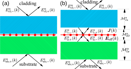
Figure 2: (color online) (a) 2D layer (red in the middle) within a multilayered structure. The incident fields are $E_{\text{cl};-}^{\alpha}(k)$ from cladding and $E_{\text{sb};+}^{\alpha}(k)$ from substrate, while the outgoing fields are $E_{\text{cl};+}^{\alpha}(k)$ and $E_{\text{sb};-}^{\alpha}(k)$. (b) An equivalent structure of (a) by formally inserting a vacuum region around the 2D layer, similar to Fig. 1. The transfer matrix ${\cal M}_{cu}^{\alpha}(k)$ is for the region from the cladding to the upper surface of the region containing the 2D layer, and ${\cal M}_{ls}^{\alpha}(k)$ is for the region from the lower surface of the region containing the 2D layer to the substrate.

In this section we consider the effects of the surrounding environment on the nonlinear optics of a 2D material, with a structure shown in Fig. 2 (a). The incident fields are $E_{\text{cl};-}^{\alpha}(k)$ from the cladding and $E_{\text{sb};+}^{\alpha}(k)$ from the substrate, while the outgoing fields are $E_{\text{cl};+}^{\alpha}(k)$ and $E_{\text{sb};-}^{\alpha}(k)$. We only consider the nonlinear optics from the 2D layer; for other layers, nonlinear radiation can be obtained from the coupled mode theory Boyd (2008) or, in an undepleted pump approximation, by the bulk medium version of these equations Sipe (1987) . To utilize the transfer matrix formalism, we slightly deform the structure into Fig. 2 (b), anticipating that we will treat the thickness of the vacuum region containing the 2D layer as vanishingly small. Now the expressions in Sec. II can be straightforwardly extended. We denote the transfer matrix for the multilayered structure from the cladding layer to the upper surface of the 2D layer region as ${\cal M}_{cu}^{\alpha}(k)$, and the transfer matrix for the multilayered structure from the lower surface of the 2D layer region to the substrate as ${\cal M}_{ls}^{\alpha}(k)$. Then we have

$$\begin{pmatrix}E_{\text{cl};+}^{\alpha}(k)\\ E_{\text{cl};-}^{\alpha}(k)\end{pmatrix} ={\cal M}_{cu}^{\alpha}(k)\begin{pmatrix}E_{1;+}^{\alpha}(k)\\ E_{1;-}^{\alpha}(k)\end{pmatrix}\,,$$ (17a)

$$\begin{pmatrix}E_{2;+}^{\alpha}(k)\\ E_{2;-}^{\alpha}(k)\end{pmatrix} ={\cal M}_{ls}^{\alpha}(k)\begin{pmatrix}E_{\text{sb};+}^{\alpha}(k)\\ E_{\text{sb};-}^{\alpha}(k)\end{pmatrix}\,,$$ (17b)

Eliminating $E_{j;\pm}^{\alpha}(k)$ from Eqs. (15), (17a), and (17b), the fields at the cladding connect with the fields at the substrate by a transfer matrix formalism as

$$\begin{pmatrix}E_{\text{cl};+}^{\alpha}(k)\\ E_{\text{cl};-}^{\alpha}(k)\end{pmatrix}={\cal M}_{cs}^{\alpha}(k)\begin{pmatrix}E_{\text{sb};+}^{\alpha}(k)\\ E_{\text{sb};-}^{\alpha}(k)\end{pmatrix}+{\cal M}_{\text{nl}}^{\alpha}(k)\begin{pmatrix}{\cal G}_{\text{2D};+}^{\alpha}(k)\\ -{\cal G}_{\text{2D};-}^{\alpha}(k)\end{pmatrix}\,,$$ (18)

with the total transfer matrix

$${\cal M}_{cs}^{\alpha}(k)={\cal M}_{cu}^{\alpha}(k){\cal M}_{\text{2D}}^{\alpha}(k){\cal M}_{ls}^{\alpha}(k)\,,$$ (19)

and a transfer matrix for the nonlinear radiation

$${\cal M}_{\text{nl}}^{\alpha}(k)={\cal M}_{cu}^{\alpha}(k)\frac{{\cal M}_{\text{2D}}^{\alpha}(k)+1}{2}\,.$$ (20)

Converting to a scattering matrix form, we obtain the outgoing fields as

$$\begin{pmatrix}E_{\text{cl};+}^{\alpha}(k)\\ E_{\text{sb};-}^{\alpha}(k)\end{pmatrix} = \begin{pmatrix}R_{cs}^{\alpha}(k)&T_{cs}^{\alpha}(k)\\ T_{sc}^{\alpha}(k)&R_{sc}^{\alpha}(k)\end{pmatrix}\begin{pmatrix}E_{\text{cl};-}^{\alpha}(k)\\ E_{\text{sb};+}^{\alpha}(k)\end{pmatrix}$$ (21)

$$+ \begin{pmatrix}1&-R_{cs}^{\alpha}(k)\\ 0&-T_{sc}^{\alpha}(k)\end{pmatrix}{\cal M}_{\text{nl}}^{\alpha}(k)\begin{pmatrix}{\cal G}_{\text{2D};+}^{\alpha}(k)\\ -{\cal G}_{\text{2D};-}^{\alpha}(k)\end{pmatrix}\,,\quad\quad$$

where the Fresnel coefficients appearing here are associated with the total transfer matrix ${\cal M}_{cs}^{\alpha}(k)$ by

$${\cal M}_{cs}^{\alpha}(k)=\frac{1}{T_{sc}^{\alpha}(k)}\begin{pmatrix}{T}_{cs}^{\alpha}(k){T}_{sc}^{\alpha}(k)-{R}_{cs}^{\alpha}(k){R}_{sc}^{\alpha}(k)&{R}_{cs}^{\alpha}(k)\\ -{R}_{sc}^{\alpha}(k)&1\end{pmatrix}\,.$$ (22)

In the absence of the nonlinear terms the results from Eq. (21) for $E_{\text{cl};+}^{\alpha}(k)$ and $E_{\text{sb};-}^{\alpha}(k)$ in terms of the Fresnel coefficients are just what one would expect. For the nonlinear radiation, the key quantity is still ${\cal G}_{\text{2D};\lambda}^{\alpha}(k)$, or equivalently the nonlinear current $\vec{{\cal J}}_{\text{nl}}(k)$, which strongly depend on the total field $\bm{E}_{\text{eff}}(k)$ at the 2D layer. Again, similar to the strategy for a suspended 2D layer, it can be found from Eqs. (3), (4), (6), (17a), and (17b) as

$$\bm{E}_{\text{eff}}(k)=\bm{E}_{\text{2D}}(k)+{\cal Q}(k)\vec{{\cal J}}(k)\,,$$ (23)

where the incident fields $\bm{E}_{\text{2D}}(k)$ at the 2D layer, and the radiation coefficients ${\cal Q}(k)$ are given in Appendix C. Equation (23) has the same structure as Eq. (7), but each term is modified to include the effects from the environment, i.e., other layers. All the results from Eq. (10a) to Eq. (11d) can be simply transferred here after replacing $\bm{E}_{\text{2D}}^{0}(k)$ and ${\cal Q}^{0}(k)$ by $\bm{E}_{2D}(k)$ and ${\cal Q}(k)$, respectively. For example, comparing to Eq. (10a), the effective field depends on the nonlinear current according to

$$\bm{E}_{\text{eff}}(k)=\left[\hat{I}-{\cal Q}(k)\eta^{(1)}(k)\right]^{-1}\left[\bm{E}_{\text{2D}}(k)+{\cal Q}(k)\vec{{\cal J}}_{\text{nl}}(k)\right]\,.\quad\quad$$ (24)

IV Results for a graphene monolayer

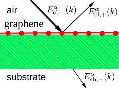
Figure 3: (color online) Illustration of a graphene-covered multilayered structure.

We illustrate our approach by considering a graphene-covered multilayered structure shown in Fig. 3. We assume there is incident light only from the cladding layer, so ${E}_{\text{sb};+}^{\alpha}(k)=0$, and we are interested in the output field ${E}_{\text{cl};+}^{\alpha}(k)$. We ignore any nonlinear sources in the multilayer, cladding, and substrate. In the widely accepted treatment for graphene the optical response in the $z$ direction is ignored, so we put $\eta_{\perp}^{(1)}(\omega)\rightarrow 0$, and assume as well that the nonlinear current has only in-plane components and responds only to the in-plane electric field components. We then require only the in-plane components of the effective fields, which we write as $\bm{E}_{\text{eff};\parallel}(k)=E_{\text{eff};s}(k)\hat{\bm{s}}(k)+E_{\text{eff};\kappa}(k)\hat{\bm{\kappa}}$, and similarly will have only an in-plane nonlinear current $\vec{{\cal J}}_{\text{nl};\parallel}(k)$. With the $z$-component of the current sheet thus ignored and the $z$-component of the effective field not required, Eq. (24) is greatly simplified to give

$$E_{\text{eff};j}(k) =\frac{E_{\text{2D};j}(k)+{\cal Q}_{jj}(k){\cal J}_{\text{nl};j}(k)}{1-{\cal Q}_{jj}(k)\eta_{\parallel}^{(1)}(k)}\,,$$ (25)

for $j=s$ or $\kappa$. Using Eq. (55a) and (55b) for $E_{\text{2D};j}(k)$, the in-plane effective electric fields are found to be

$$E_{\text{eff};s}(k) = [1+R_{cs}^{s}(k)]\left[E_{\text{cl};-}^{s}(k)-\frac{\widetilde{\omega}}{w_{0}(k)}{\cal J}_{\text{nl};s}(k)\right]\,,\quad\quad$$ (26)

$$E_{\text{eff};\kappa}(k) = [1-R_{cs}^{p}(k)]\left[E_{\text{cl};-}^{p}(k)-{\cal J}_{\text{nl};\kappa}(k)\right]\frac{w_{0}(k)}{\widetilde{\omega}}\,.\quad\quad,$$ (27)

and from the transfer matrices the total reflectivity $R_{cs}^{\alpha}(k)$ is found to be

$$R_{cs}^{\alpha}(k) =r^{\alpha}(k)+\frac{t^{\alpha}(k)R_{ls}^{\alpha}(k)t^{\alpha}(k)}{1-R_{ls}^{\alpha}(k)r^{\alpha}(k)}$$

$$=\frac{\tau^{\alpha}}{\dfrac{1}{1+\tau^{\alpha}R_{ls}^{\alpha}(k)}+\left[\dfrac{\widetilde{\omega}}{w_{0}(k)}\right]^{\tau^{\alpha}}\eta_{\parallel}^{(1)}(\omega)}-\tau^{\alpha}\,.$$ (28)

Here $R_{ls}^{\alpha}(k)$ is the reflection coefficient without the presence of graphene, $\tau^{s}=1$, and $\tau^{p}=-1$; in the second expression the result is displayed explicitly in terms of the linear conductivity of the 2D layer. Finally, from Eq. (21) the output fields can then be written into terms of the nonlinear current as

$${E}_{\text{cl},+}^{\alpha}(k) =R_{cs}^{\alpha}(k){E}_{\text{cl},-}^{\alpha}(k)$$

$$-[1+\tau^{\alpha}R_{cs}^{\alpha}(k)]\frac{\widetilde{\omega}}{w_{0}(k)}\vec{{\cal J}}_{\text{nl};\parallel}(k)\cdot\hat{\bm{e}}_{0;+}^{\alpha}\,.$$ (29)

According to earlier results Cheng et al. (2015a); *Phys.Rev.B_93_39904_2016_Cheng; Cheng et al. (2017), the nonlinear currents up to the third order terms are

$$\vec{{\cal J}}_{\text{nl};\parallel}(k) =2\int\frac{dk_{1}}{(2\pi)^{3}}\Bigg{\{}{\cal S}_{M}^{xxyy}(\omega_{1},\omega_{a})[\bm{\kappa}_{1}\times\bm{E}_{\text{eff};\parallel}(k_{1})]\times\bm{E}_{\text{eff};\parallel}(k_{a})+{\cal S}_{Q}^{xxyy}(\omega_{1},\omega_{a})[\bm{E}_{\text{eff};\parallel}(k_{1})\bm{\kappa}_{1}\cdot\bm{E}_{\text{eff};\parallel}(k_{a})$$

$$\hskip 28.45274pt+\bm{\kappa}_{1}\bm{E}_{\text{eff};\parallel}(k_{1})\cdot\bm{E}_{\text{eff};\parallel}(k_{a})]+{\cal S}_{Q}^{xyxy}(\omega_{1},\omega_{a})\bm{\kappa}_{1}\cdot\bm{E}_{\text{eff};\parallel}(k_{1})\bm{E}_{\text{eff};\parallel}(k_{a})\Bigg{\}}$$

$$+3\int\frac{dk_{1}dk_{2}}{(2\pi)^{6}}\eta^{(3);xxyy}(\omega_{1},\omega_{2},\omega_{b})\bm{E}_{\text{eff};\parallel}(k_{1})\bm{E}_{\text{eff};\parallel}(k_{2})\cdot\bm{E}_{\text{eff};\parallel}(k_{b})\,,$$ (30)

with $k_{a}=k-k_{1}$ and $k_{b}=k-k_{1}-k_{2}$. For the second order response, ${\cal S}_{Q}^{xxyy}$ and ${\cal S}_{Q}^{xyxy}$ are response coefficients associated with the quadrupole-like contribution, and ${\cal S}_{M}^{xxyy}$ is a response coefficient associated with the magnetic dipole-like contribution; they are related to the parameters $S_{Q/M}^{dabc}$ defined earlier Cheng et al. (2017) by ${\cal S}=S/(2c\epsilon_{0})$. For later use, the components along the $x$-direction of the conductivity tensors are given by

$$\eta_{2}(k_{1},k_{2}) \equiv \eta^{(2);xxx}(k_{1},k_{2})$$ (31a)

$$= {\cal S}^{xxxx}(\omega_{1},\omega_{2})\kappa_{1}^{c}+{\cal S}^{xxxx}(\omega_{2},\omega_{1})\kappa_{2}^{c}\,,$$

$$\eta_{3}(\omega_{1},\omega_{2},\omega_{3}) \equiv \eta^{(3);xxxx}(\omega_{1},\omega_{2},\omega_{3})$$ (31b)

$$= \eta^{(3);xxyy}(\omega_{1},\omega_{2},\omega_{3})+\eta^{(3);xxyy}(\omega_{2},\omega_{3},\omega_{1})$$

$$+\eta^{(3);xxyy}(\omega_{3},\omega_{1},\omega_{2})\,,$$

with ${\cal S}^{xxxx}(\omega_{1},\omega_{2})=2{\cal S}_{Q}^{xxyy}(\omega_{1},\omega_{2})+{\cal S}_{Q}^{xyxy}(\omega_{1},\omega_{2})$.

We note that the argument $k=(\bm{\kappa},\omega)$ of ${E}_{\text{cl};-}^{\alpha}(k)$ varies continuously, and thus the equations can describe a pulse of light with arbitrary polarization incident on only a finite region of the structure shown in Fig. 3. Here we consider simple cases with incident plane waves at discrete $k_{j}$, which is performed by the transformation

$${E}_{\text{cl};-}^{\alpha}(k)\to(2\pi)^{3}\sum_{j}\delta(k-k_{j}){E}_{\text{cl};-}^{\alpha}(k_{j})\,.$$ (32)

All new $k_{j}$ generated by the nonlinearity are then also discrete.

In the following two subsections, we explicitly give the perturbation formulas for SHG, THG, and PFC.

IV.1 SHG and THG

In this section we derive the formulas for the SHG and THG signals, induced by a single $p-$polarized incident laser beam with amplitude ${E}_{\text{cl};-}^{p}(k)$, as shown in Fig. 3. We list all perturbative quantities with respect to the incident fields. The perturbative effective fields at the graphene layer are given as

$$\bm{E}_{\text{eff};\parallel}^{(1)}(k) ={\cal P}(k)E_{\text{cl};-}^{p}(k)\hat{\bm{\kappa}}\,,$$

$$\bm{E}_{\text{eff};\parallel}^{(2)}(k) =-{\cal P}(k){\cal J}_{\text{nl};\kappa}^{(2)}(k)\hat{\bm{\kappa}}\,,$$

with

$${\cal P}(k)=[1-R_{cs}^{p}(k)]\frac{w_{0}(k)}{\widetilde{\omega}}\,.$$ (33)

The perturbative current responses for SHG and THG are

$$\vec{{\cal J}}_{\text{nl};\parallel}^{(2)}(2k) =\eta_{2}(k,k)\hat{\bm{\kappa}}[E_{\text{eff};\kappa}^{(1)}(k)]^{2}\,,$$ (34a)

$$\vec{{\cal J}}_{\text{nl};\parallel}^{(3)}(3k) =\eta_{3}(\omega,\omega,\omega)\hat{\bm{\kappa}}[E_{\text{eff};\kappa}^{(1)}(k)]^{3}$$

$$+2\eta_{2}(k,2k)\hat{\bm{\kappa}}E_{\text{eff};\kappa}^{(1)}(k)E_{\text{eff};\kappa}^{(2)}(2k)\,.$$ (34b)

Substituting them into Eq. (29), the radiation fields for SHG and THG only include the $p$-polarized components as

$$E_{\text{cl};+}^{p}(2k) =\eta_{\text{SHG}}(k)\beta_{\text{SHG}}(k)[E_{\text{cl};-}^{p}(k)]^{2}\,,$$ (35a)

$$E_{\text{cl};+}^{p}(3k) =\eta_{\text{THG}}(k)\beta_{\text{THG}}(k)[E_{\text{cl};-}^{p}(k)]^{3}\,,$$ (35b)

with $\eta_{\text{SHG}}(k)=\eta_{2}(k,k)$ and

$$\eta_{\text{THG}}(k)=\eta_{3}(\omega,\omega,\omega)-2\eta_{2}(k,2k){\cal P}(2k)\eta_{2}(k,k)\,.$$ (36)

Here all quantities indicated by $\beta$ are dimensionless structure factors, which include the effects from the lower layers of the structure. They are given by

$$\beta_{\text{SHG}}(k) =\left[1-R_{cs}^{p}(2k)\right][{\cal P}(k)]^{2}\,,$$ (37a)

$$\beta_{\text{THG}}(k) =\left[1-R_{cs}^{p}(3k)\right][{\cal P}(k)]^{3}\,.$$ (37b)

As an example, we consider these structure related quantities for a THG experimental setup as used by Kumar et al. Kumar et al. (2013). The layer structure is shown in Fig. 4(a); it is composed of air cladding/graphene/300 nm thick SiO₂/silicon substrate. The incident light is at $\hbar\omega=0.72$ eV, with an incident angle $\theta$ or in-plane wavevector $\bm{\kappa}=\widetilde{\omega}\sin\theta\hat{\bm{x}}$. The dielectric constants we used are listed in Table 1, and the linear conductivity of graphene is taken as $\sigma_{0}$.

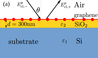
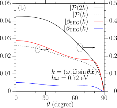
Figure 4: (color online) (a) Illustration of the structure analyzed, (b) the angle dependence of $|\beta_{\text{SHG}}(k)|$, $|\beta_{\text{THG}}(k)|$, $|{\cal P}(2k)|$, and $|{\cal P}(k)|$. The $y$-axis of $|{\cal P}|$s is at the right, as indicated.

	$\varepsilon(\omega)$	$\varepsilon(2\omega)$	$\varepsilon(3\omega)$
SiO2	2.08	2.11	2.13
Si	12.01	$13.27+0.022i$	$16.03+0.189i$
	$R_{cs}^{p}(k_{\perp})$	$R_{cs}^{p}(2k_{\perp})$	$R_{cs}(3k_{\perp})$
	$0.74+0.001i$	$0.57-0.007i$	$0.71+0.006i$
graphene
$\eta_{2}(k,k)/\sin\theta$		$(1.1-0.6i)\times 10^{-15}$ m/V
$\eta_{2}(k,2k)/\sin\theta$		$(1.2-0.53)\times 10^{-16}$ m/V
$\eta_{3}(\omega,\omega,\omega)$		$(6.4+1.6i)\times 10^{-22}$ m2/V2

Table 1: The values for the dielectric constants of SiO₂ and Si (taken from website ‘http://refractiveindex.info/”), the total reflection coefficient at normal incidence, and the optical conductivities of graphene. The nonlinear conductivities of graphene are taken from earlier work [Cheng et al., 2015a; *Phys.Rev.B_93_39904_2016_Cheng, Cheng et al., 2017], with parameters $\mu=0.2$ eV, $\Gamma_{e}=\Gamma_{i}=33$ meV, and $T=300$ K. The linear conductivity of graphene is approximated as $\sigma_{0}$.

In Fig. 4 (b), we plot the $\theta$ dependence of $|\beta_{\text{SHG}}(k)|$, $|\beta_{\text{THG}}(k)|$, and $|{\cal P}(2k)|$. As the incident angle is increased, they decrease. At normal incidence, the values of $|\beta_{\text{SHG}}|$ and $|\beta_{\text{THG}}|$ are of the order of $10^{-2}$ and $10^{-3}$, respectively. Both of them are much smaller than $1$, which means the layer structure greatly reduces the harmonic radiation signal. This is because the value of $|{\cal P}(k)|$ is less than 0.3, and as it is raised to a power of 2 and 3 the resulting values are much smaller. At normal incidence $k=k_{\perp}=(\bm{0},\omega)$, the structure factors can be written as $\beta_{\text{SHG}}(k_{\perp})={\cal P}(2k_{\perp})[{\cal P}(k_{\perp})]^{2}\approx 2.9\times 10^{-2}$ and $\beta_{\text{THG}}(k_{\perp})={\cal P}(3k_{\perp})[{\cal P}(k_{\perp})]^{3}\approx 5\times 10^{-3}$. Compared to a suspended graphene, where both of them are around unity, the layers underneath reduce the harmonic radiation significantly. The dependence of these structure factors on the substrate reflection coefficient is clear.

Equation (36) includes the contribution to the THG coefficients from the cascaded processes, with the values of $|{\cal P}(2k)|$ smaller than 0.5. By checking graphene’s conductivities listed in Table 1, we find the contribution from the cascaded second order processes to the THG process are about 9 orders of magnitude smaller than the direct third order response. This is not surprising, because the second order response in graphene is induced by theoretically forbidden optical processes and is a weak effect, which gives very small $\eta_{2}(k,k)$ and $\eta_{2}(k,2k)$. And ${\cal P}(2k)$ does not undergo any resonance for the structure and parameters used in the experiment.

Following a similar strategy, in the next section we look at parametric frequency conversion.

IV.2 Parametric frequency conversion

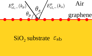
Figure 5: (color online) Illustration of the structure in the experiment of Constant et al.Constant et al. (2015).

The PFC process occurs when the structure is excited by two laser beams: one is a pump beam at $k_{p}$, the other is a signal beam at $k_{s}$. We are interested in the output light at a difference frequency $k_{d}=k_{p}-k_{s}$, which is generated by the second order nonlinearity, and in the idler light at $k_{i}=2k_{p}-k_{s}$, which is generated by the third order nonlinearity. In the experiment of Constant et al. Constant et al. (2015), due to a carefully designed structure and appropriate incident angles the light at $k_{d}$ can be evanescent and on resonance with the plasmon modes of the whole structure. As shown in Fig. 5, the structure is composed of graphene covered SiO₂. For simplicity, we consider that the $p$-polarized incident beams are in the same incident plane, with in-plane wave vectors $\bm{\kappa}_{p}=\kappa_{p}\hat{\bm{\kappa}}_{p}$ and $\bm{\kappa}_{s}=\kappa_{s}(-\hat{\bm{\kappa}}_{p})$, and with frequencies $\omega_{p}>\omega_{s}$.

In a calculation similar to that of the previous section, we find the output fields at $k_{d}$ and $k_{i}$ are

$$E_{\text{cl};+}^{p}(k_{d}) =-2\eta_{\text{DFG}}(k_{p},k_{s})\beta_{\text{DFG}}(k_{p},k_{s})$$

$$\times E_{\text{cl};-}^{p}(k_{p})[E_{\text{cl};-}^{p}(k_{s})]^{\ast}\,,$$ (38a)

$$E_{\text{cl};+}^{p}(k_{i}) =-3\eta_{\text{PFC}}(k_{p},k_{s})\beta_{\text{PFC}}(k_{p},k_{s})$$

$$\times[E_{\text{cl};-}^{p}(k_{p})]^{2}[E_{\text{cl};-}^{p}(k_{s})]^{\ast}\,,$$ (38b)

The prefactors $2$ and $3$ come from the permutation of the incident field components, and the minus signs appear due to the opposite incident directions of these two beams. The terms related to the conductivities are $\eta_{\text{DFG}}(k_{p},k_{s})=\eta_{2}(k_{p},-k_{s})$ and $\eta_{\text{PFC}}(k_{p},k_{s})=\eta_{3}(\omega_{p},\omega_{p},-\omega_{s})+\eta_{3c}(k_{p},k_{s})$. The term $\eta_{3c}$ includes the contribution from the cascaded second order processes to the third order response, and is given as

$$\eta_{3c}(k_{p},k_{s}) =-\frac{4}{3}\eta_{2}(k_{p},k_{d}){\cal P}(k_{d})\eta_{2}(k_{p},-k_{s})\,.$$ (39)

Here only the cascaded process involving the light at $k_{d}$ is taken into account. The dimensionless structure factors are

$$\beta_{\text{DFG}}(k_{p},k_{s}) =[1-R_{cs}^{p}(k_{d})]{\cal P}(k_{p})[{\cal P}(k_{s})]^{\ast}\,,$$ (40a)

$$\beta_{\text{PFC}}(k_{p},k_{s}) =[1-R_{cs}^{p}(k_{i})][{\cal P}(k_{p})]^{2}[{\cal P}(k_{s})]^{\ast}\,.$$ (40b)

Besides involving a product of two second order conductivities, the cascaded process coefficient $\eta_{3c}(k_{p},k_{s})$ in Eq. (39) is also proportional to the term ${\cal P}(k_{d})$. This illustrates how the structure underneath the graphene can be used to tune the cascaded process: In the experiment by Constant et al. Constant et al. (2015), this term is maximized by matching $k_{d}$ with the surface plasmon polariton (SPP) resonance of the entire structure. In an ideal case, when all losses are ignored, $R_{cs}^{p}(k_{d})$ diverges at the resonance; with losses, its value becomes finite, but still very large. As an illustration, this can be clearly seen in Fig. 6(a). For the parameters of graphene we choose the chemical potential as $\mu=1.11$ eV, the relaxation parameters $\Gamma_{i}=\Gamma_{e}=1$ meV, and assume zero temperature. The very high chemical potential, which can be realized by a gate voltage Jiang et al. (2018), is chosen to satisfy resonant conditions in calculating the second order and third order conductivities. The calculation is made for signal light at wavelength $615$ nm ($\widetilde{\omega}_{s}=10.22~{}\mu$m^-1) with an incident angle $\theta_{s}=125^{\circ}$, and pump light at wavelength $\lambda_{p}$ varying from $547$ nm to $615$ nm ($\widetilde{\omega}_{p}$ varying from $11.49~{}\mu$m^-1 to $10.22~{}\mu$m^-1) with an incident angle $\theta_{p}=15^{\circ}$. As the pump light wavelength varies, the in-plane wave vector and frequency of the light at $k_{d}=k_{p}-k_{s}$ vary along the black line in Fig. 6(a). The linear conductivities for graphene are shown in Fig. 6(c). The maximal value of $|R_{cs}^{p}(k_{d})|$ along the black line in Fig. 6(a) is about $41$, and occurs for $\widetilde{\omega}_{p}=11.22~{}\mu$m^-1where the SPP is excited.

We first check the structure factor for PFC, which is shown in Fig. 6(b). As $\lambda_{p}$ varies, $|\beta_{\text{PFC}}|$ is at the order of 0.05 and changes only slightly. This small value results mostly because of the oblique incidence of the light, as captured by the term $w_{0}(k)/\widetilde{\omega}$ in the expression of Eq. (33) for ${\cal P}(k)$. For the difference frequency generation, the structure factor $|\beta_{\text{DFG}}|$ can be as large as $10$ at the SPP resonance at $\widetilde{\omega}_{p}=11.22\mu$m^-1. Obviously, the light at $k_{d}$ is evanescent in air; however, it is could be detected by the use of near field techniques.

Interestingly, the cascaded second order processes can exceed the direct third order process at certain frequencies, mainly because in this case we have very large second order conductivities as well as a SPP resonance, as shown in Fig. 6 (d) and 6 (e). There are in total three possible resonances for the conductivities with varying

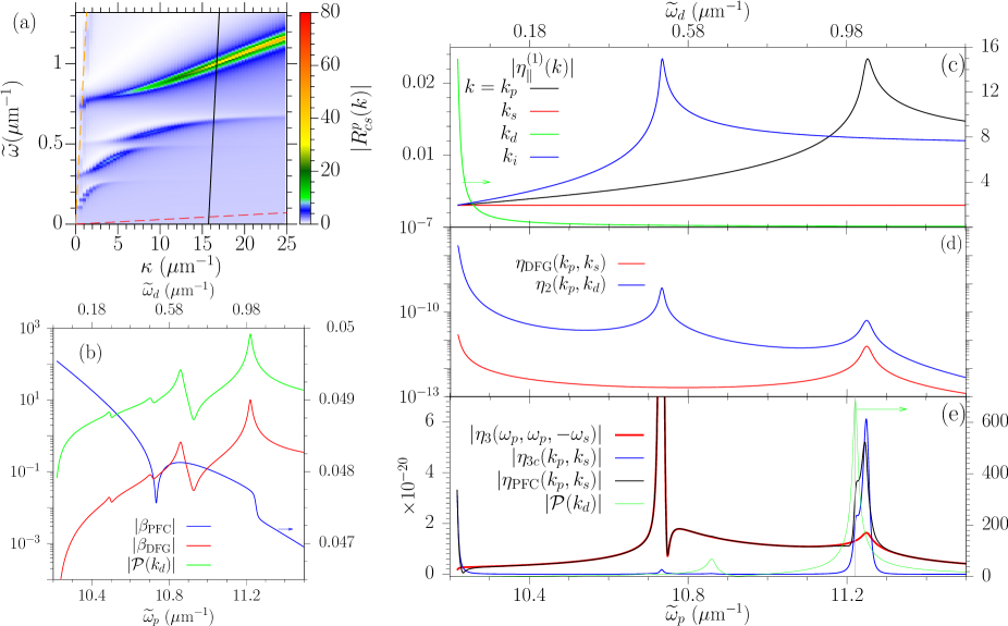
Figure 6: (color online) (a) $k$-dependence of the reflection coefficients. The orange dashed line is the light line, the red dashed line is the graphene dispersion, and the black line is the trajectory of $k_{d}$ when $\lambda_{p}$ varies from 547 nm to 615 nm for $\lambda_{s}=615$ nm, $\theta_{s}=125^{\circ}$, and $\theta_{p}=15^{\circ}$. (b) The structure factors $\beta_{\text{PFC}}(k_{p},k_{s})$, $\beta_{\text{DFG}}(k_{p},k_{s})$, and ${\cal P}(k_{d})$. (c) $\eta_{\parallel}^{(1)}(k)$ for $k=k_{p}$, $k_{s}$, $k_{d}$, and $k_{i}$. (d) $\eta_{\text{DFG}}(k_{p},k_{s})$ and $\eta_{2}(k_{p},k_{d})$. (e) $\eta_{\text{PFC}}(k_{p},k_{s})$, $\eta_{3c}(k_{p},k_{s})$, $\eta_{3}(\omega_{p},\omega_{p},-\omega_{s})$, and ${\cal P}(k_{d})$. All curves indicated by horizontal arrows use the right $y$-axis. In the calculation, the parameters for graphene are taken as $\mu=1.11$ meV, $\Gamma_{i}=\Gamma_{e}=1$ meV, and $T=0$ K.

$\widetilde{\omega}_{p}$, the first is at $\widetilde{\omega}_{A}=[\widetilde{\omega}_{s}+2\mu/(\hbar c)]/2=10.73\mu$m^-1, corresponding to the condition $2\hbar\omega_{A}-\hbar\omega_{s}=2\mu$; the second is at $\widetilde{\omega}_{B}=\widetilde{\omega}_{s}$; and the third is at $\widetilde{\omega}_{C}=2\mu/(\hbar c)=11.25\mu$m^-1, corresponding to the condition $\hbar\omega_{C}=2\mu$. Our calculations show that $\eta_{2}(k_{p},-k_{s})$ shows peaks at $\widetilde{\omega}_{B}$ and $\widetilde{\omega}_{C}$; $\eta_{2}(k_{p},k_{d})$ shows peaks at $\widetilde{\omega}_{A}$, $\widetilde{\omega}_{B}$, and $\widetilde{\omega}_{C}$; and $\eta_{3}(\omega_{p},\omega_{p},-\omega_{s})$ shows peaks at $\widetilde{\omega}_{A}$ and $\widetilde{\omega}_{c}$. For $\widetilde{\omega}_{p}$ around $\widetilde{\omega}_{B}$ and $\widetilde{\omega}_{C}$, the cascaded second order processes dominate because of the very large second order conductivities. But there is another peak for $\widetilde{\omega}_{p}\sim 11.22~{}\mu$m, located at the same peak position of ${\cal P}(k_{d})$, which is induced by the SPP resonance.

All these calculations are for ideal parameters. For higher temperature, larger relaxation parameters, and smaller chemical potential, the second order conductivities can be reduced greatly, as well the value of $\eta_{3c}(k_{p},k_{s})$. Because the graphene layer is put in an asymmetric environment, an additional contribution to the second order nonlinearity can arise from the interface effect. However, it contributes only to the out-of-plane tensor components, which are ignored in the usual model for graphene.

V Conclusion

We have derived the basic equations for analyzing the linear and nonlinear optics of graphene and other 2D materials in layered structures. For linear optics, we obtained the Fresnel coefficients of a suspended 2D layer. Complementing existing work in the literature, these coefficients take into account the optical response along the out-of-plane direction of the 2D layers, which is usually ignored, so they can be used to extract the out-of-plane linear conductivity components from experimental data. In the nonlinear regime, we derived an equation for the total electric field at the 2D material including the feedback radiation of its own sheet current density. After combining this with current response theory, which is widely adopted for calculating the conductivities, a set of consistent equations for the total field and the current can be obtained; after solving them either analytically or numerically, the nonlinear radiation can be found. We also derived the perturbative expressions at weak incident light beams. We discussed how the structures themselves affect the output field intensity. For some experimental scenarios the structures can reduce the radiation by several orders of magnitude, compared to that for a suspended sample. Our results can serve as a starting point for further nonlinear optical investigations of graphene or 2D materials in layered structures.

Appendix A Notations

In a homogeneous medium with dielectric constant $\varepsilon(\omega)$, the electric fields can be written as

$$\bm{E}(z;\bm{R},t) = \int_{0}^{\infty}\frac{d\omega}{2\pi}\bm{E}(z;\bm{R},\omega)e^{-i\omega t}+c.c.\,,$$ (41)

$$\bm{E}(z;\bm{R},\omega) = \int\frac{d\bm{\kappa}}{(2\pi)^{2}}\bm{E}(z;\bm{\kappa},\omega)e^{i\bm{\kappa}\cdot\bm{R}}\,,$$ (42)

with $\bm{R}=x\hat{\bm{x}}+y\hat{\bm{y}}$. Throughout this work, we use a compact notation $k=(\bm{\kappa},\omega)$, and so $\bm{E}(z;\bm{\kappa},\omega)=\bm{E}(z;k)$. The fields can be decomposed into upward and downward propagating (or evanescent) fields,

$${\bm{E}}(z;k)=\sum_{\lambda=\pm}{\bm{E}}_{\lambda}(k)e^{i\lambda w(k)z}\,,$$ (43)

with $s$- and $p$-polarized components

$${\bm{E}}_{\lambda}(k)=\sum_{\alpha=s,p}{E}_{\lambda}^{\alpha}(k)\hat{\bm{e}}_{\lambda}^{\alpha}(k)\,.$$ (44)

The polarization vectors, $\hat{\bm{e}}_{\lambda}^{\alpha}(k)$ with $\alpha=s,p$ for the field polarization and $\lambda=+,-$ for the propagation direction, are defined by

$$\hat{\bm{e}}_{\pm}^{s}(k) \equiv \hat{\bm{s}}(k)=\hat{\bm{\kappa}}\times\hat{\bm{z}}\,,$$ (45)

$$\hat{\bm{e}}_{\pm}^{p}(k) \equiv \hat{\bm{p}}_{\pm}(k)=\frac{\kappa\hat{\bm{z}}\mp w(k)\hat{\bm{\kappa}}}{\sqrt{\varepsilon(\omega)}\widetilde{\omega}}\,.$$ (46)

where $w(k)=\sqrt{\varepsilon(\omega)\widetilde{\omega}^{2}-\kappa^{2}}$ with $\widetilde{\omega}=\omega/c$, is taken such that $\text{Im}[w]\geq 0$, with $\text{Re}[w]>0$ if $\text{Im}[w]=0$. The polarization vectors are in general complex quantities; for propagating fields in lossless materials, their directions are shown in Fig. 1. Although these vectors satisfy $\hat{\bm{s}}(k)\cdot\hat{\bm{s}}(k)=1$ and $\hat{\bm{p}}_{\pm}(k)\cdot\hat{\bm{p}}_{\pm}(k)=1$, the “length” $\sqrt{\hat{\bm{p}}_{\pm}(k)\cdot[\hat{\bm{p}}_{\pm}(k)]^{\ast}}$ can be far larger than unity for an evanescent field.

To identify different regions or layers, we will use an extra subscript $j$ in $E_{j;\lambda}^{\alpha}(z;k)$, $w_{j}(k)$, $\hat{\bm{e}}_{j;\lambda}^{\alpha}(k)$, and so on.

Appendix B Green function method for a sheet current density

For a sheet current density $\bm{J}(z;k)$ embedded in a homogeneous medium with dielectric constant $\varepsilon(\omega)$, the radiation field can be calculated using a Green function strategy Sipe (1987) as

$$\bm{E}_{\text{ind}}(z;k)=\int G(z-z^{\prime};k)\cdot\frac{\bm{J}(z^{\prime};k)}{2c\epsilon_{0}}dz^{\prime}\,,$$ (47)

with

$$G(z;k) = -\frac{\tilde{\omega}}{w(k)}[\hat{\bm{s}}(k)\hat{\bm{s}}(k)+\hat{\bm{p}}_{+}(k)\hat{\bm{p}}_{+}(k)]\theta(z)e^{iw(k)z}$$ (48)

$$- \frac{\tilde{\omega}}{w(k)}[\hat{\bm{s}}(k)\hat{\bm{s}}(k)+\hat{\bm{p}}_{-}(k)\hat{\bm{p}}_{-}(k)]\theta(-z)e^{-iw(k)z}$$

$$- 2i\frac{\hat{\bm{z}}\hat{\bm{z}}}{\widetilde{\omega}\varepsilon(\omega)}\delta(z)\,,$$

In the region $z>0$ of the setup in Fig. 1, the induced field $\bm{E}_{\text{ind}}(z>0;k)$ only propagate upwards, and it can be written as

$$\bm{E}_{\text{ind}}(z>0;k)=\sum_{\alpha=s,p}{\cal F}_{+}^{\alpha}(k)e^{iw(k)z}\hat{\bm{e}}_{+}^{\alpha}(k)$$ (49)

with ${\cal F}_{+}^{\alpha}$ given in Eq. (5). Then the upward fields $\bm{E}_{1;+}(k)$ include two contributions: one is from the incident fields $\bm{E}_{2;+}(k)$ that is propagated from the region $z<0$, as if the sheet current density were absent; the other is the induced field ${\cal F}_{+}^{\alpha}(k)$. Then we get Eq. (3). Similarly, we can get Eq. (4).

Appendix C Incident field $\bm{E}_{\text{eff}}(k)$ at the 2D layer and the radiation coefficients ${\cal Q}(k)$

For a 2D layer inside a multilayered structure, it is convenient to write the incident field $\bm{E}_{\text{2D}}$ at the 2D layer in a coordinate formed by $\{\hat{\bm{s}},\hat{\bm{\kappa}},\hat{\bm{z}}\}$ as

$$\bm{E}_{\text{2D}}=E_{\text{2D};s}\hat{\bm{s}}+E_{\text{2D};\kappa}\hat{\bm{\kappa}}+E_{\text{2D};z}\hat{\bm{z}}\,.$$ (50)

Without causing any confusion, the $k$-dependence of each quantity is implicitly shown. From Eqs. (3), (4), (6), (17a), and (17b), the effective field $\bm{E}_{\text{eff}}$ at the 2D layer can be written into Eq. (23) with

$$E_{\text{2D};s} =\frac{[\overline{R}_{cs}^{s}-R_{cu}^{s}][1+R_{uc}^{s}]+T_{cu}^{s}T_{uc}^{s}}{T_{cu}^{s}}E_{\text{cl};-}^{s}+\frac{[1+R_{uc}^{s}]\overline{T}_{cs}^{s}}{T_{cu}^{s}}E_{\text{sb};+}^{s}\,,$$ (51a)

$$E_{\text{2D};\kappa} =\left\{\frac{-[\overline{R}_{cs}^{p}-R_{cu}^{p}][1-R_{uc}^{p}]+T_{cu}^{p}T_{uc}^{p}}{T_{cu}^{p}}E_{\text{cl};-}^{p}+\frac{[-1+R_{uc}^{p}]\overline{T}_{cs}^{p}}{T_{cu}^{p}}E_{\text{sb};+}^{p}\right\}\frac{w_{0}}{\widetilde{\omega}}\,,$$ (51b)

$$E_{\text{2D};z} =\left\{\frac{[\overline{R}_{cs}^{p}-R_{cu}^{p}][1+R_{uc}^{p}]+T_{cu}^{p}T_{uc}^{p}}{T_{cu}^{p}}E_{\text{cl};-}^{p}+\frac{[1+R_{uc}^{p}]\overline{T}_{cs}^{p}}{T_{cu}^{p}}E_{\text{sb};+}^{p}\right\}\frac{\kappa}{\widetilde{\omega}}\,.$$ (51c)

Here $\overline{T}^{\alpha}$ and $\overline{R}^{\alpha}$ are the Fresnel coefficient for the structure without the presence of 2D material, which are given from

$${\cal M}_{cu}^{\alpha}{\cal M}_{ls}^{\alpha}=\frac{1}{\overline{T}_{sc}^{\alpha}}\begin{pmatrix}\overline{T}_{cs}^{\alpha}\overline{T}_{sc}^{\alpha}-\overline{R}_{cs}^{\alpha}\overline{R}_{sc}^{\alpha}&\overline{R}_{cs}^{\alpha}\\ -\overline{R}_{sc}^{\alpha}&1\end{pmatrix}\,;$$ (52a)

while $$R T$$ and are the Fresnel coefficients for the substrate multilayers, which are given as

$${\cal M}_{cu}^{\alpha} =\frac{1}{{T}_{uc}^{\alpha}}\begin{pmatrix}{T}_{cu}^{\alpha}{T}_{uc}^{\alpha}-{R}_{cu}^{\alpha}{R}_{uc}^{\alpha}&{R}_{cu}^{\alpha}\\ -{R}_{uc}^{\alpha}&1\end{pmatrix}\,.$$ (52b)

Along the directions $\{\hat{\bm{s}},\hat{\bm{\kappa}},\hat{\bm{z}}\}$, the radiation coefficient is a tensor matrix with a form ${\cal Q}={\cal Q}_{ss}\hat{\bm{s}}\hat{\bm{s}}+{\cal Q}_{\kappa\kappa}\hat{\bm{\kappa}}\hat{\bm{\kappa}}+{\cal Q}_{zz}\hat{\bm{z}}\hat{\bm{z}}+{\cal Q}_{\kappa z}\hat{\bm{\kappa}}\hat{\bm{z}}+{\cal Q}_{z\kappa}\hat{\bm{z}}\hat{\bm{\kappa}}$ with elements

$${\cal Q}_{ss} =-\frac{\widetilde{\omega}}{w_{0}}\frac{[\overline{R}_{cs}^{s}-R_{cu}^{s}][1+R_{uc}^{s}]+T_{cu}^{s}T_{uc}^{s}}{T_{cu}^{s}}\frac{1+R_{uc}^{s}}{T_{uc}^{s}}\,,$$ (53a)

$${\cal Q}_{\kappa\kappa} =-\frac{w_{0}}{\widetilde{\omega}}\frac{-[\overline{R}_{cs}^{p}-R_{cu}^{p}][1-R_{uc}^{p}]+T_{cu}^{p}T_{uc}^{p}}{T_{cu}^{p}}\frac{1-R_{uc}^{p}}{T_{uc}^{p}}\,,$$ (53b)

$${\cal Q}_{zz} =-\frac{\kappa^{2}}{w_{0}\widetilde{\omega}}\frac{[\overline{R}_{cs}^{p}-R_{cu}^{p}][1+R_{uc}^{p}]+T_{cu}^{p}T_{uc}^{p}}{T_{cu}^{p}}\frac{1+R_{uc}^{p}}{T_{uc}^{p}}\,,$$ (53c)

$${\cal Q}_{\kappa z} =-{\cal Q}_{z\kappa}=-\frac{\kappa}{\widetilde{\omega}}\frac{[R_{cu}^{p}-\overline{R}_{cs}^{p}]\{1-[R_{uc}^{p}]^{2}\}+R_{uc}^{p}T_{cu}^{p}T_{uc}^{p}}{T_{cu}^{p}T_{uc}^{p}}\,.$$ (53d)

We give these quantities for two special cases:
(1) For a suspended system, all reflection coefficients associated with additional material are zero and all transmission coefficients are $1$. Therefore we can get the effective incident field at the 2D layer is

$$\bm{E}_{\text{2D}}^{0} =[E_{1;-}^{s}+E_{2;+}^{s}]\hat{\bm{s}}+\frac{w_{0}}{\widetilde{\omega}}\left[E_{1;-}^{p}-E_{2;+}^{p}\right]\hat{\bm{\kappa}}$$

$$+\frac{\kappa}{\widetilde{\omega}}\left[E_{1;-}^{p}+E_{2;+}^{p}\right]\hat{\bm{z}}\,,$$ (54a)

and the radiation coefficient matrix becomes diagonal,

$${\cal Q}^{0}=-\frac{\widetilde{\omega}}{w_{0}}\hat{\bm{s}}\hat{\bm{s}}-\frac{w_{0}}{\widetilde{\omega}}\hat{\bm{\kappa}}\hat{\bm{\kappa}}-\frac{\kappa^{2}}{w_{0}\widetilde{\omega}}\hat{\bm{z}}\hat{\bm{z}}\,.$$ (54b)

(2) When the 2D layer is put directly on top of a substrate, we have $R_{cu}^{\alpha}=R_{uc}^{\alpha}=0$, and $T_{cu}^{\alpha}=T_{uc}^{\alpha}=1$. The effective field is

$$E_{\text{2D};s} =[1+R_{ls}^{s}]E_{\text{cl};-}^{s}+T_{ls}^{s}E_{\text{sb};+}^{s}\,,$$ (55a)

$$E_{\text{2D};\kappa} =\left\{[1-R_{ls}^{p}]E_{\text{cl};-}^{p}-T_{ls}^{p}E_{\text{sb};+}^{s}\right\}\frac{w_{0}}{\widetilde{\omega}}\,,$$ (55b)

$$E_{\text{2D};z} =\left\{[1+R_{ls}^{p}]E_{\text{cl};-}^{p}+T_{ls}^{p}E_{\text{sb};+}^{s}\right\}\frac{\kappa}{\widetilde{\omega}}\,,$$ (55c)

with $\overline{R}_{cs}^{\alpha}=R_{ls}^{\alpha}$ and $\overline{T}_{cs}^{\alpha}=T_{ls}^{\alpha}$ being the Fresnel coefficient associated with the lower multilayered structure. The ${\cal Q}$ is then given as

$${\cal Q}_{ss} =-\frac{\widetilde{\omega}}{w_{0}}\left[1+R_{ls}^{s}\right]\,,$$ (56a)

$${\cal Q}_{\kappa\kappa} =-\frac{w_{0}}{\widetilde{\omega}}\left[1-R_{ls}^{p}\right]\,,$$ (56b)

$${\cal Q}_{zz} =-\frac{\kappa^{2}}{w_{0}\widetilde{\omega}}\left[R_{ls}^{p}+1\right]\,,$$ (56c)

$${\cal Q}_{\kappa z} =-{\cal Q}_{z\kappa}=\frac{\kappa}{\widetilde{\omega}}{R}_{ls}^{p}\,.$$ (56d)

References

- Bonaccorso et al. (2010) F. Bonaccorso, Z. Sun, T. Hasan, and A. C. Ferrari, Nat. Photon. 4, 611 (2010).
- Nair et al. (2008) R. R. Nair, P. Blake, A. N. Grigorenko, K. S. Novoselov, T. J. Booth, T. Stauber, N. M. R. Peres, and A. K. Geim, Science 320, 1308 (2008).
- Low and Avouris (2014) T. Low and P. Avouris, ACS Nano 8, 1086 (2014).
- Garcǐa de Abajo (2014) F. J. Garcǐa de Abajo, ACS Photonics 1, 135 (2014).
- Ooi and Tan (2017) K. J. A. Ooi and D. T. H. Tan, Proc. R. Soc. A 473, 20170433 (2017).
- Glazov and Ganichev (2014) M. Glazov and S. Ganichev, Phys. Rep. 535, 101 (2014).
- Sun et al. (2016) Z. Sun, A. Martinez, and F. Wang, Nat. Photon. 10, 227 (2016).
- Autere et al. (2018) A. Autere, H. Jussila, Y. Dai, Y. Wang, H. Lipsanen, and Z. Sun, Adv. Mater. , 1705963 (2018).
- Pinto et al. (2009) H. Pinto, R. Jones, J. P. Goss, and P. R. Briddon, J. Phys. Condens. Matter 21, 402001 (2009).
- Liu et al. (2011a) H. Liu, Y. Liu, and D. Zhu, J. Mater. Chem. 21, 3335 (2011a).
- Ni et al. (2016) G. X. Ni, L. Wang, M. D. Goldflam, M. Wagner, Z. Fei, A. S. McLeod, M. K. Liu, F. Keilmann, B. Özyilmaz, A. H. C. Neto, J. Hone, M. M. Fogler, and D. N. Basov, Nat. Photon. 10, 244 (2016).
- Novoselov et al. (2004) K. S. Novoselov, A. K. Geim, S. V. Morozov, D. Jiang, Y. Zhang, S. V. Dubonos, I. V. Grigorieva, and A. A. Firsov, Science 306, 666 (2004).
- Hendry et al. (2010) E. Hendry, P. J. Hale, J. Moger, A. K. Savchenko, and S. A. Mikhailov, Phys. Rev. Lett. 105, 097401 (2010).
- Xia et al. (2014) F. Xia, H. Wang, D. Xiao, M. Dubey, and A. Ramasubramaniam, Nat. Photon. 8, 899 (2014).
- Vermeulen et al. (2016a) N. Vermeulen, J. L. Cheng, J. E. Sipe, and H. Thienpont, IEEE J. Sel. Top. Quantum Electron. 22, 347 (2016a).
- Bao et al. (2009) Q. Bao, H. Zhang, Y. Wang, Z. Ni, Y. Yan, Z. X. Shen, K. P. Loh, and D. Y. Tang, Adv. Funct. Mater. 19, 3077 (2009).
- Liu et al. (2011b) M. Liu, X. Yin, E. Ulin-Avila, B. Geng, T. Zentgraf, L. Ju, F. Wang, and X. Zhang, Nature 474, 64 (2011b).
- Liu et al. (2012) M. Liu, X. Yin, and X. Zhang, Nano Lett. 12, 1482 (2012).
- Ooi et al. (2014) K. J. A. Ooi, L. K. Ang, and D. T. H. Tan, Appl. Phys. Lett. 105, 111110 (2014).
- Ooi et al. (2016) K. J. A. Ooi, J. L. Cheng, J. E. Sipe, L. K. Ang, and D. T. H. Tan, APL Photon. 1, 046101 (2016).
- Jiang et al. (2018) T. Jiang, D. Huang, J. Cheng, X. Fan, Z. Zhang, Y. Shan, Y. Yi, Y. Dai, L. Shi, K. Liu, C. Zeng, J. Zi, J. E. Sipe, Y.-R. Shen, W.-T. Liu, and S. Wu, Nat. Photon. 12, 430 (2018).
- Kumar et al. (2013) N. Kumar, J. Kumar, C. Gerstenkorn, R. Wang, H.-Y. Chiu, A. L. Smirl, and H. Zhao, Phys. Rev. B 87, 121406 (2013).
- Hong et al. (2013) S.-Y. Hong, J. I. Dadap, N. Petrone, P.-C. Yeh, J. Hone, and R. M. Osgood, Jr., Phys. Rev. X 3, 021014 (2013).
- Säynätjoki et al. (2013) A. Säynätjoki, L. Karvonen, J. Riikonen, W. Kim, S. Mehravar, R. A. Norwood, N. Peyghambarian, H. Lipsanen, and K. Kieu, ACS Nano 7, 8441 (2013).
- Soavi et al. (2018) G. Soavi, G. Wang, H. Rostami, D. G. Purdie, D. De Fazio, T. Ma, B. Luo, J. Wang, A. K. Ott, D. Yoon, S. A. Bourelle, J. E. Muench, I. Goykhman, S. Dal Conte, M. Celebrano, A. Tomadin, M. Polini, G. Cerullo, and A. C. Ferrari, Nat. Nano. 13, 583 (2018).
- Dean and van Driel (2009) J. J. Dean and H. M. van Driel, Appl. Phys. Lett. 95, 261910 (2009).
- Dean and van Driel (2010) J. J. Dean and H. M. van Driel, Phys. Rev. B 82, 125411 (2010).
- Bykov et al. (2012) A. Y. Bykov, T. V. Murzina, M. G. Rybin, and E. D. Obraztsova, Phys. Rev. B 85, 121413 (2012).
- An et al. (2013) Y. Q. An, F. Nelson, J. U. Lee, and A. C. Diebold, Nano Lett. 13, 2104 (2013).
- An et al. (2014) Y. Q. An, J. E. Rowe, D. B. Dougherty, J. U. Lee, and A. C. Diebold, Phys. Rev. B 89, 115310 (2014).
- Lin et al. (2014) K.-H. Lin, S.-W. Weng, P.-W. Lyu, T.-R. Tsai, and W.-B. Su, Appl. Phys. Lett. 105, 151605 (2014).
- Xing et al. (2010) G. Xing, H. Guo, X. Zhang, T. C. Sum, and C. H. A. Huan, Opt. Express 18, 4564 (2010).
- Wu et al. (2011) R. Wu, Y. Zhang, S. Yan, F. Bian, W. Wang, X. Bai, X. Lu, J. Zhao, and E. Wang, Nano Lett. 11, 5159 (2011).
- Yang et al. (2011) H. Yang, X. Feng, Q. Wang, H. Huang, W. Chen, A. T. S. Wee, and W. Ji, Nano Lett. 11, 2622 (2011).
- Zhang et al. (2012) H. Zhang, S. Virally, Q. Bao, L. K. Ping, S. Massar, N. Godbout, and P. Kockaert, Opt. Lett. 37, 1856 (2012).
- Gu et al. (2012) T. Gu, N. Petrone, J. F. McMillan, A. van der Zande, M. Yu, G. Q. Lo, D. L. Kwong, J. Hone, and C. W. Wong, Nat. Photon. 6, 554 (2012).
- Vermeulen et al. (2016b) N. Vermeulen, D. Castelló-Lurbe, J. L. Cheng, I. Pasternak, A. Krajewska, T. Ciuk, W. Strupinski, H. Thienpont, and J. Van Erps, Phys. Rev. Appl. 6, 044006 (2016b).
- Dremetsika et al. (2016) E. Dremetsika, B. Dlubak, S.-P. Gorza, C. Ciret, M.-B. Martin, S. Hofmann, P. Seneor, D. Dolfi, S. Massar, P. Emplit, and et al., Opt. Lett. 41, 3281 (2016).
- Vermeulen et al. (2018) N. Vermeulen, D. Castelló-Lurbe, M. Khoder, I. Pasternak, A. Krajewska, T. Ciuk, W. Strupinski, J. L. Cheng, H. Thienpont, and J. V. Erps, Nature Comm. 9, 2675 (2018).
- Sun et al. (2010) D. Sun, C. Divin, J. Rioux, J. E. Sipe, C. Berger, W. A. de Heer, P. N. First, and T. B. Norris, Nano Lett. 10, 1293 (2010).
- Sun et al. (2012) D. Sun, J. Rioux, J. E. Sipe, Y. Zou, M. T. Mihnev, C. Berger, W. A. de Heer, P. N. First, and T. B. Norris, Phys. Rev. B 85, 165427 (2012).
- Demetriou et al. (2016) G. Demetriou, H. T. Bookey, F. Biancalana, E. Abraham, Y. Wang, W. Ji, and A. K. Kar, Opt. Express 24, 13033 (2016).
- Cheng et al. (2014) J. L. Cheng, N. Vermeulen, and J. E. Sipe, New J. Phys. 16, 053014 (2014).
- Cheng et al. (2016a) J. L. Cheng, N. Vermeulen, and J. E. Sipe, New J. Phys. 18, 029501 (2016a).
- Cheng et al. (2015a) J. L. Cheng, N. Vermeulen, and J. E. Sipe, Phys. Rev. B 91, 235320 (2015a).
- Cheng et al. (2016b) J. L. Cheng, N. Vermeulen, and J. E. Sipe, Phys. Rev. B 93, 039904 (2016b).
- Cheng et al. (2015b) J. L. Cheng, N. Vermeulen, and J. E. Sipe, Phys. Rev. B 92, 235307 (2015b).
- Soh et al. (2016) D. B. S. Soh, R. Hamerly, and H. Mabuchi, Phys. Rev. A 94, 023845 (2016).
- Rostami and Polini (2016) H. Rostami and M. Polini, Phys. Rev. B 93, 161411 (2016).
- Mikhailov (2016) S. A. Mikhailov, Phys. Rev. B 93, 085403 (2016).
- Wang et al. (2016) Y. Wang, M. Tokman, and A. Belyanin, Phys. Rev. B 94, 195442 (2016).
- Cheng et al. (2017) J. L. Cheng, N. Vermeulen, and J. E. Sipe, Sci. Rep. 7, 43843 (2017).
- Mikhailov (2017) S. A. Mikhailov, Phys. Rev. B 95, 085432 (2017).
- Marini et al. (2017) A. Marini, J. D. Cox, and F. J. García de Abajo, Phys. Rev. B 95, 125408 (2017).
- Rostami et al. (2017) H. Rostami, M. I. Katsnelson, and M. Polini, Phys. Rev. B 95, 035416 (2017).
- Avetissian and Mkrtchian (2018) H. K. Avetissian and G. F. Mkrtchian, Phys. Rev. B 97, 115454 (2018).
- Constant et al. (2015) T. J. Constant, S. M. Hornett, D. E. Chang, and E. Hendry, Nat. Phys. 12, 124 (2015).
- Cox and Javier García de Abajo (2014) J. D. Cox and F. Javier García de Abajo, Nat. Comm. 5, 5725 (2014).
- Boyd (2008) R. W. Boyd, Nonlinear Optics, 3rd ed. (Academic, 2008).
- Zhao et al. (2016) M. Zhao, Z. Ye, R. Suzuki, Y. Ye, H. Zhu, J. Xiao, Y. Wang, Y. Iwasa, and X. Zhang, Light Sci. App. 5, e16131 (2016).
- Vincenti et al. (2013) M. A. Vincenti, D. de Ceglia, M. Grande, A. D’Orazio, and M. Scalora, Opt. Lett. 38, 3550 (2013).
- Vincenti et al. (2014) M. A. Vincenti, D. de Ceglia, M. Grande, A. D’Orazio, and M. Scalora, Phys. Rev. B 89, 165139 (2014).
- Savostianova and Mikhailov (2015) N. A. Savostianova and S. A. Mikhailov, Appl. Phys. Lett. 107, 181104 (2015).
- Savostianova and Mikhailov (2017) N. A. Savostianova and S. A. Mikhailov, Opt. Express 25, 3268 (2017).
- Gorbach and Ivanov (2016) A. V. Gorbach and E. Ivanov, Phys. Rev. A 94, 013811 (2016).
- Gorbach (2013) A. V. Gorbach, Phys. Rev. A 87, 013830 (2013).
- Yao et al. (2014) X. Yao, M. Tokman, and A. Belyanin, Phys. Rev. Lett. 112, 055501 (2014).
- Tao et al. (2015) J. Tao, Z. Dong, J. K. W. Yang, and Q. J. Wang, Opt. Express 23, 7809 (2015).
- (69) J. L. Cheng, J. E. Sipe, and C. Guo, unpublished.
- Sipe (1987) J. E. Sipe, J. Opt. Soc. Am. B 4, 481 (1987).
- Ando et al. (2002) T. Ando, Y. Zheng, and H. Suzuura, J. Phys. Soc. Jpn. 71, 1318 (2002).
- Gusynin and Sharapov (2006) V. P. Gusynin and S. G. Sharapov, Phys. Rev. B 73, 245411 (2006).