Some Statistical Problems with High Dimensional Financial data

Abstract

For high dimensional data some of the standard statistical techniques do not work well. So modification or further development of statistical methods are necessary. In this paper we explore these modifications. We start with important problem of estimating high dimensional covariance matrix. Then we explore some of the important statistical techniques such as high dimensional regression, principal component analysis, multiple testing problems and classification. We describe some of the fast algorithms that can be readily applied in practice.

1 Introduction

A high degree of interdependence among modern financial systems, such as firms or banks, is captured through modeling by a network $G(V,E)$, where each node in $V$ represents a financial institution and an edge in $E$ stands for dependence between two such institutions. The edges are determined by calculating the correlation coefficient between asset prices of pairs of financial institutions. If the sample pairwise correlation coefficient is greater than some predefined threshold then an edge is formed between corresponding nodes. This network model can be useful to answer important questions on the financial market, such as determining clusters or sectors in the market, uncovering possibility of portfolio diversification or investigating the degree distribution boginski2005 , vandewalle2001 . See figure 1 for illustration of one such network. Using correlation coefficients to construct the economic or financial network has a serious drawback. If one is interested in direct dependence of two financial institutions the high observed correlation may be due to the effect of other institutions. Therefore a more appropriate measure to investigate direct dependence is partial correlation. Correlation and partial correlation coefficients are related to covariance and inverse covariance matrix respectively. Therefore in order to have meaningful inference on the complex system of financial network, estimation of covariance matrix accurately is of utmost importance. In this paper we investigate how inference based on covariance matrix for high dimensional data can be problematic and how to solve the problem.

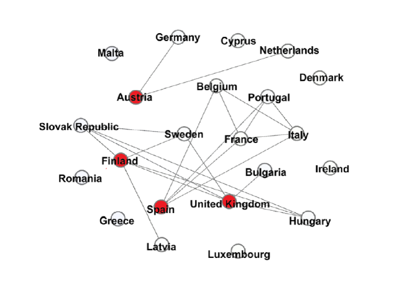
Figure 1: Network topology of European economies in post-euro period as described in papadimitriou2014european .

The rest of the paper is organized as follows. In section 2 we discuss the distribution of eigenvalues of covariance matrix. In section 3 the problem and possible solution of covariance matrix estimation is discussed. Section 4 deals with estimation of precision matrix. Section 5 and 6 deals with multiple testing procedure and high dimensional regression problem respectively. We discuss high dimensional principal component analysis and several classification algorithms in section 7 and 8.

2 Distribution of Eigenvalues

2.1 Eigenvalues of Covariance Matrix

In multivariate statistical theory, the sample covariance matrix is the most common and undisputed estimator because it is unbiased and has good large sample properties with growing number of observations when number of variables is fixed. But if the ratio of the number of variables ($p$) and the number of observations ($n$) is large, then sample covariance does not behave as expected. It can be showen that if $p$ grows at the same rate as $n$ i.e. $\nicefrac{{p}}{{n}}\rightarrow y\!>0)$ the sample covariance matrix becomes inconsistent and therefore can not be relied upon stein1956 . In Figure 2 eigenvalues of population covariance matrix and sample covariance matrix are plotted for different values of $p$ and $n$ where the population covariance matrix is the identity matrix. It is evident that the true and sample spectra differ a lot as the ratio $\nicefrac{{p}}{{n}}$ grows. So for high dimensional data ($\nicefrac{{p}}{{n}}\rightarrow y>0$) there is a need to find an improved estimator.

Even though the sample eigenvalues are not consistent anymore, the limiting distribution of eigenvalues of the sample covariance matrix and the connection it has with the limiting eigenvalue distribution of population covariance matrix are of importance. Determining the limiting spectral distribution can be very useful to test the underlying assumption of the model. In this section we will very briefly discuss some results of random matrix theory that answers this kind of questions. Throughout we will denote the ratio $p/n$ as $y_{n}$.

2.2 Marchenko Pastur Law and Tracy Widom Law

Suppose that $\{x_{ij}\}$ are iid Gaussian variables with variance $\sigma^{2}$. If $\nicefrac{{p}}{{n}}\rightarrow y>0$ then the empirical spectral distribution (distribution function of eigenvalues) of sample covariance matrix $S_{n}$converges almost surely to the distribution F with the density

$$f(x) =\frac{1}{2\pi\sigma^{2}yx}\sqrt{(b-x)(x-a)}I(a\leq x\leq b)$$

if $y<1$, where $a=a(y)=\sigma^{2}(1-\sqrt{y})^{2}$ and $b=b(y)=\sigma^{2}(1+\sqrt{y})^{2}$. If $y$ $>1$ It will take additional positive mass $1-\frac{1}{y}$ at 0.

$\sigma$ is called the scale parameter. The distribution is known as Marchenko-Pastur distribution.

If $\nicefrac{{p}}{{n}}\rightarrow 0$ then empirical spectral distribution of $W_{n}=\sqrt{\frac{n}{p}(S_{n}-\sigma^{2}I})$ converges almost surely to the semicircle law with density:

$$f(x)=\frac{1}{2\pi\sigma^{2}}\sqrt{4\sigma^{2}-x^{2}}I(|x|\leq 2\sigma)$$

Although the sample eigenvalues are not consistent estimator, the limiting spectral distribution is related to the population covariance matrix in a particular way.

Also if $p\rightarrow\infty$ and $n\rightarrow\infty$ such that $\frac{p}{n}\rightarrow y>0$, then $\frac{\lambda_{1}-\mu_{np}}{\sigma_{np}}\stackrel{{\scriptstyle\mathcal{L}}}{{\rightarrow}}W_{1}$where $\lambda_{1}$ is the largest eigenvalue of sample covariance $\mu_{np}=(\sqrt{n}+\sqrt{p})^{2}$ and $\sigma_{np}=(\sqrt{n}+\sqrt{p})(\frac{1}{\sqrt{n}}+\frac{1}{\sqrt{p}})^{\frac{1}{3}}$ and $W_{1}$ is Tracy-Widom Law distribution.

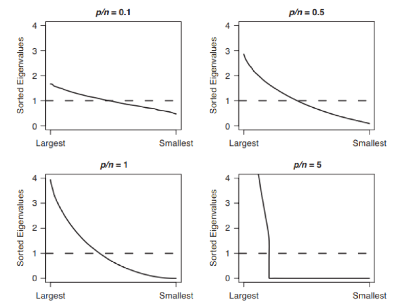
Figure 2: Plot of true (dotted line) and sample (solid line) eigenvalues.

3 Covariance Matrix Estimator

3.1 Stein’s Approach

We see from figure 2 that the sample eigenvalues can differ a lot from the population eigenvalues. Thus shrinking the eigenvalues to a central value is a reasonable approach to take. Such an estimator was proposed by Stein stein1956inadmissibility and takes the following form:

$$\hat{\Sigma}=\hat{\Sigma}(S)=P\psi(\Lambda)P^{\prime}$$

where $\Lambda=diag(\lambda_{1},\lambda_{2},...,\lambda_{p})$ and $\psi(\Lambda)$ is also a diagonal matrix. If $\psi(\lambda_{i})=\lambda_{i}\forall i$ then $\hat{\Sigma}$ is the usual estimator $S$. In this approach the eigen vectors are kept as it is, but the eigenvalues are shrink towards a central value. As the eigen vectors are not altered or regularized this estimator is called rotation equivariant covariance estimator. To come up with a choice of $\psi$, we can use entropy loss function

$$L=\mathrm{tr}(\hat{\Sigma}\Sigma^{-1})-\mathrm{log}(\hat{\Sigma}\Sigma^{-1})-p$$

or Frobeneous loss function

$$L_{2}=\mathrm{tr}(\hat{\Sigma}\Sigma^{-1}-I)^{2}.$$

Under entropy risk ($=E_{\Sigma}(L)$), we have $\psi(\lambda_{i})=\frac{\lambda_{i}n}{\alpha_{i}}$ where

$$\alpha_{i}=(n-p+1+2\lambda_{i}\Sigma_{i\neq j}\frac{1}{\lambda_{i}-\lambda_{j}}).$$

The only problem with this estimator is that some of the essential properties of eigenvalues, like monotonicity and nonnegativity, are not guaranteed. Some modifications can be adopted in order to force the estimator to satisfy those conditions (see Lin and naul2016 ). An algorithm was proposed to avoid such undesirable situations by pooling adjacent estimators together in Stein1975 . In this algorithm first the negative $\alpha_{i}$’s are pooled together with previous values until it becomes positive and then to keep the monotonicity intact, the estimates ($\psi^{\prime}s$) are pooled together pairwise.

3.2 Ledoit-Wolf type Estimator

As an alternative to the above mentioned method, the empirical Bayes estimator can also be used to shrink the eigenvalues of sample covariance matrix. haff1980 proposed to estimate $\Sigma$ by

$$\hat{\Sigma}=\frac{np-2n-2}{n^{2}p}\utilde{\alpha}I+\frac{n}{n+1}S,$$

where $\utilde{\alpha}=(\mathrm{det}(S))^{\nicefrac{{1}}{{p}}}$. This estimator is a linear combination of $S$ and $I$ which is reasonable because although $S$ is unbiased, it is highly unstable for high dimensional data and $\alpha I$ has very little variability with possibly high bias. Therefore a more general form of estimator would be

$$\hat{\Sigma}=\alpha_{1}T+\alpha_{2}S$$

where $T$ is a positive definite matrix and $\alpha_{1}$ (shrinkage intensity parameter), $\alpha_{2}$ can be determined by minimising the loss function. For example ledoit2004 used

$$L(\hat{\Sigma},\Sigma)=\frac{1}{p}\mathrm{tr}(\hat{\Sigma}-\Sigma)^{2}$$

to obtain a consistent estimator with $T=I$. A trade off between bias and variance is achieved through the value of shrinkage parameter. In figure 3, bias, variance and MSE are plotted against shrinkage parameter. The optimum value of shrinkage intensity is that for which MSE is minimum.

It can be shown that if there exists $k_{1}$ and $k_{2}$ independent of $n$ such that $\nicefrac{{p}}{{n}}\leq k_{1}$ and $\frac{1}{p}\sum_{i=1}^{p}\mathrm{E}[Y_{i}]^{8}\leq k_{2}$ where $Y_{i}$ is the $i$-th element of any row of the matrix of principal components of $X$ and if

$$\lim_{n\rightarrow\infty}\frac{p^{2}}{n^{2}}\times\frac{\sum_{(i,j,k,l)\in Q_{n}}(\mathrm{Cov}[Y_{i}Y_{j},Y_{k}Y_{l}])^{2}}{\mathrm{cardinality}(Q_{n})}=0$$

where $Q_{n}$ denotes the set of all quadruples made of four distinct integers between $1$ and $p$, then the following estimator $S_{n}^{*}$ (a convex combination of $I$ and $S$) is consistent for $\Sigma$, see ledoit2004 :

$$S_{n}^{*}=\frac{b_{n}^{2}}{d_{n}^{2}}m_{n}I_{n}+\frac{d_{n}^{2}-b_{n}^{2}}{d_{n}^{2}}S_{n}$$

where $X_{k.}$ is the $k$th row of $X$ and

$$m_{n} =\frac{1}{p}\mathrm{tr}(S_{n}^{{}^{\prime}}I_{n})$$

$$d_{n}^{2} =\|S_{n}-m_{n}I_{n}\|^{2}$$

$$b_{n}^{2} =\mathrm{min}(d_{n}^{2},\frac{1}{n^{2}}\sum_{k=1}^{n}\|X_{k.}^{{}^{\prime}}X_{k.}-S_{n}\|^{2}).$$

The first condition clearly deals with the interplay between sample size, dimension and moments whereas the second one deals with the dependence structure. For $\nicefrac{{p}}{{n}}\rightarrow 0$ the last condition for dependence structure can be trivially verified as a consequence of the assumption on moments. This estimate is also computationally easy to work with. In fact as $S$ is still unbiased estimator one possible way to reduce the variance is to use bootstrap-dependent techniques like bagging. But that is far more computationally demanding compared to this method.

With the additional assumption that $\mathrm{var}(\frac{\sum_{i=1}^{p}Y_{i}^{2}}{p})$ is bounded as $n\rightarrow\infty$, ledoit2004 showed that

$$lim_{n\rightarrow\infty}[E||S_{n}-\Sigma_{n}||^{2}-\frac{p}{n}(m_{n}^{2}+var(\frac{\sum_{i=1}^{p}Y_{i}^{2}}{p}))]=0$$

This result implies that expected loss of sample covariance matrix, although bounded, does not usually vanish. Therefore consistency of usual sample covariance matrix is achieved only when $\frac{p}{n}\rightarrow 0$ or $m_{n}^{2}+\mathrm{var}(\frac{\sum_{i=1}^{p}Y_{i}^{2}}{p})\rightarrow 0.$ In the latter case most of the random variables are asymptotically degenerate. The difference between these two cases is that in the first, the number of variables is very less compared to $n$ and in the latter $O(n)$ degenerate variables are augmented with the earlier lot. Both of these essentially indicate sparsity.

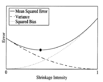
Figure 3: Plot for Error vs shirnkage intensity ledoit2004

A more general target matrix $T$ can be used instead $I$. For example, under Gaussian distribution, if $T=\nicefrac{{\mathrm{tr}(S)}}{{p}}I$, $\alpha_{1}=\lambda$ (intensity parameter) and $\alpha_{2}=1-\lambda$, then optimal shrinkage intensity is

$$min(\frac{\sum_{i=1}^{p}||x_{i}x_{i}^{\prime}-S||_{F}^{2}}{n^{2}[tr(S^{2})-tr^{2}(S)/p]},1)$$

which implies that the shrinkage estimator is a function of the sufficient statistics $S$ and therefore can be further improved upon by using Rao-Blackwell theorem chen2009shrinkage . The resulting estimator becomes $\lambda_{RBLW}T+(1-\lambda_{RBLW})S$ where

$$\lambda_{RBLW}=\frac{\frac{n-2}{n}tr(S)+tr^{2}(S)}{(n+2)[tr(S^{2})-\frac{tr^{2}(S)}{p}]}$$

If we take $T=\mathrm{Diag}(S)$, that is, the diagonal elements of $S$ then the optimal intensity that minimises $E[\|\hat{\Sigma}-\Sigma\|^{2}]$ can be estimated as

$$\frac{\frac{1}{n}(\hat{a}_{2}+p\hat{a}_{12})-\frac{2}{n}\hat{a}_{2}*}{\frac{n+1}{n}\hat{a}_{2}+\frac{p}{n}\hat{a}_{1}^{2}-\frac{n+2}{n}\hat{a}_{2}*}$$

where $\hat{a}_{1}=\nicefrac{{1}}{{p}}\mathrm{tr}(S)$, $\hat{a}_{2}=\frac{n^{2}}{(n-1)(n+2)}\frac{1}{p}[\mathrm{tr}S^{2}-\frac{1}{n}(\mathrm{tr}S)^{2}],$ $\hat{a}_{2}^{*}=\frac{n}{n+2}\mathrm{tr}(T^{2})/p$ as shown infisher2011 . schafer2005 chose the shrinkage parameter to be

$$\lambda*=\frac{\sum_{i=1}^{p}\hat{\mathrm{var}}(s_{i})-\hat{\mathrm{cov}}(t_{i},s_{i})-\hat{\mathrm{Bias}}(s_{i})(t_{i}-s_{i})}{\sum_{i=1}^{p}(t_{i}-s_{i})^{2}}.$$

Along with conventional target matrix ($I$) they used five other target matrices summarised in the following Table.

Table 1

Target A: "diagonal, unit variance” 0 estimated parameters $t_{ij}=\begin{cases}1&if\ i=j\\ 0&if\ i\neq j\end{cases}$ $\hat{\lambda}^{*}=\frac{\sum_{i\neq j}\bar{var}(s_{ij})+\sum_{i=j}\bar{var}(s_{ii})}{\sum_{i\neq j}s_{ij}{}^{2}+\sum_{i}(s_{ii}-1)^{2}}$	Target B: “diagonal, common variance” 1 estimated parameter: $v$ $t_{ij}=\begin{cases}v=avg(s_{ii})&if\ i=j\\ 0&if\ i\neq j\end{cases}$ $\hat{\lambda}^{*}=\frac{\sum_{i\neq j}\bar{var}(s_{ij})+\sum_{i}\bar{var}(s_{ii})}{\sum_{i\neq j}s_{ij}^{2}+\sum_{i}(s_{ij}-v)^{2}}$
Target C: "common (co)variance” 2 estimated parameters: $v,\!c$ $t_{ij}=\begin{cases}v=avg(s_{ii})&if\ i=j\\ c=avg(s_{ij})&if\ i\neq j\end{cases}$ $\hat{\lambda}^{*}=\frac{\sum_{i\neq j}\bar{var}(s_{ij})+\sum_{i=j}\bar{var}(s_{ii})}{\sum_{i\neq j}(s_{ij}-c)^{2}+\sum_{i}(s_{ij}-v)^{2}}$	Target D: "diagonal, unequal variance ” $p$ estimated parameters: $s_{ii}$ $t_{ij}=\begin{cases}v=s_{ii}&if\ i=j\\ 0&if\ i\neq j\end{cases}$ $\hat{\lambda}^{*}=\frac{\sum_{i\neq j}\bar{var}(s_{ij})}{\sum_{i\neq j}s_{ij}^{2}}$
Target E: “perfect positive correlation” $p$ estimated parameters: $s_{ij}$ $t_{ij}=\begin{cases}s_{ii}&if\ i=j\\ \sqrt{s_{ij}s_{ji}}&if\ i\neq j\end{cases}$ $f_{ij}=\frac{1}{2}\{\sqrt{\frac{s_{jj}}{s_{ii}}}\hat{Cov}(s_{ii},s_{ij})+\sqrt{\frac{s_{ii}}{s_{jj}}}\hat{Cov}(s_{jj},s_{ij})\}$ $\hat{\lambda}^{*}=\frac{\sum_{i\neq j}\bar{Var}(s_{ij})-f_{ij}}{\sum_{i\neq j}(s_{ij}-\sqrt{s_{ii}s_{jj}})^{2}}$	Target F: “constant correlation” $p+1$ estimated parameters, $s_{ii},\!\bar{r}$ $t_{ij}=\begin{cases}s_{ii}&if\ i=j\\ \bar{r}\sqrt{s_{ij}s_{ji}}&if\ i\neq j\end{cases}$ $f_{ij}=\frac{1}{2}\{\sqrt{\frac{s_{jj}}{s_{ii}}}\hat{Cov}(s_{ii},s_{ij})+\sqrt{\frac{s_{ii}}{s_{jj}}}\hat{Cov}(s_{jj},s_{ij})\}$ $\hat{\lambda}^{*}=\frac{\sum_{i\neq j}\bar{Var}(s_{ij})-\bar{r}f_{ij}}{\sum_{i\neq j}(s_{ij}-\bar{r}\sqrt{s_{ii}s_{jj}})^{2}}$

3.3 Element-wise Regularization

Under the assumption of sparsity, some element-wise regularization methods can be used. In contrast to ledoit2004 type of estimator, where only the eigenvalues were shrunk, here both eigenvalues and vectors are regularised. We will first discuss popular methods like Banding and Tapering which assume some order between the variables and as a result, the estimator is not invariant under permutation of variables. So this is useful for time-dependent data.

Banding

The idea behind banding is that the variables are ordered in such a way that elements of the covariance matrix, further away from the main diagonal, are negligible. An $l-$banded covariance matrix is defined as $B(S_{l})=[s_{ij}I(|i-j|\leq l)]$, where $S=[s_{ij}]$ is the $p\times p$ sample covariance matrix and $l$ $(\leq p)$ is band length, determined through cross validation. One can question- which kind of population covariance matrix can be well approximated by Banded sample covariance matrix. Intuitively, such a matrix should have decaying entries as one moves away from the main diagonal. bickel2008covariance showed that the population covariance can be well approximated uniformly over the following class of matrices: $\{\Sigma:\ \mathrm{max}_{j}\sum_{i}|\sigma_{ij}|\!I(i-j\geq k)\leq C.k^{-\alpha},\mathrm{and}\ 0<\epsilon\leq\lambda_{\mathrm{min}}(\Sigma)<\lambda_{\mathrm{max}}(\Sigma)\leq\epsilon^{-1}\}$, where $C$ is a constant and $\alpha$ captures the rate of decay of the entries $\sigma_{ij}$ as $i$ goes away from $j$. Although $p$ is large, if $\mathrm{log}(p)$ is very small compared to $n$, that is, $\frac{\mathrm{log}(p)}{n}\rightarrow 0$, then such a $\Sigma$ can be well-approximated by accurately chosen band length and the error in approximation depends on $\mathrm{log}(p)/n$ and $\alpha$. Same result holds also for the precision matrix. Banded covariance estimation procedure does not guarantee positive definiteness.

Tapering

Tapering the covariance matrix is another possible way and it can preserve positive definiteness. $T(S)=S\circ T$ is a tapered estimator where $S$ is the sample covariance matrix, $T$ is the tapering matrix and ‘$\circ$’ denotes the Hadamard product (element-wise product). Properties of Hadamard product suggest that $T(S)$ is positive definite if $T$ is so. The banded covariance matrix is a special case of this with $T=((1_{[|i-j|\leq l}))$, which is not positive definite.

Thresholding

The most widely applicable element-wise regularization method is defined through Thresholding Operator. The regularized estimator is $T_{\lambda}(S)=((s_{ij}I(s_{ij})>\lambda)\thinspace))$, where $S=((s_{ij}))$ is the sample covariance matrix and $\lambda>0$ is the threshold parameter. $\lambda$ can be determined through cross validation. Although it is much simpler than other methods, like penalized lasso, it has one problem. The estimator preserves symmetry but not positive definiteness. With Gaussian assumption, consistency of this estimator can be shown uniformly over a class $\{\Sigma:\ \sigma_{ii}\leq C,\ \sum_{j=1}^{p}|\sigma_{ij}|^{q}\leq s_{0}(p),\ \forall\thinspace i\}$ with $0\leq q\leq 1$, $\nicefrac{{\mathrm{log}(p)}}{{n}}=o(1)$ and $\lambda=M\sqrt{\frac{log(p)}{n}}$for sufficiently large $M$ bickel2008covariance . For $q=0$ the condition $\sum_{j=1}^{p}|\sigma_{ij}|^{q}\leq s_{0}(p)$ reduces to $\sum_{j=1}^{p}I(\sigma_{ij}\neq 0)\leq s_{0}(p).$ The rate of convergence is dependent on the dimension ($p$), sample size ($n$) and $s_{0}$, the determining factor of the number of nonzero elements in $\Sigma$. Similar result can be shown for precision matrix. For non-Gaussian case, we need some moment conditions in order to achieve consistency result bickel2008covariance .

The result goes through for a larger class of thresholding operators. One such is called generalized thresholding operators with the following three properties:

1. $|s_{\lambda}(x)|\leq|x|$ (shrinkage)

2. $s_{\lambda}(x)=0$ for $|x|\leq\lambda$(thresholding)

3. $|s_{\lambda}(x)-x|\leq\lambda$(constraint on amount of shrinkage)

Apart from being consistent under suitable conditions discussed earlier, if variance of each variable is bounded then this operator is also “sparsistent” i.e. able to identify true zero entries of population covariance matrix with probability tending to one.

For both thresholding and generalized thresholding operators $\lambda$ is fixed for all entries of the matrix. An adaptive threshold estimator can be developed cai2011adaptive to have different parameters for different entries where

$$\lambda_{ij}\propto\sqrt{\frac{log(p)}{n}\hat{var}(Y_{i}-\mu_{i})(Y_{j}-\mu_{j})}$$

3.4 Approximate Factor Model

Sometimes the assumption of sparsity is too much to demand. For such situations estimation methods of a larger class of covariance matrices is required. A simple extension is possible to the class of matrices that can be decomposed into sum of low rank and sparse matrix: $\Sigma=FF^{T}+\Psi$, where $F$ is low rank and $\Psi$ is sparse matrix. Due to similarity with Factor model where $\Psi$ is diagonal, this model is called approximate factor model. To estimate $\Sigma$, one can decompose $S$ similarly as, $S=\sum_{i=1}^{q}\hat{\lambda}_{i}\hat{e}_{i}\hat{e}_{i}^{T}+R$, where the first part involves the first $q$ principal components and the second part is residual. As $R$ is sparse we can now use thresholding/adaptive thresholding operators to estimate it chamberlain1982arbitrage .

3.5 Positive Definiteness

Sometimes positive definiteness of the estimator is required in order to be used in classification or covariance regularised regression. As we have discussed thresholding estimators do not guarantee positive definite estimator. In the following section we will describe a couple of methods to achieve that. One possible way is to replace the negative eigenvalues in eigen decomposition of $\hat{\Sigma}$ by zero. But this manipulation destroys the sparse nature of the covariance matrix. An alternative way is necessary that will ensure sparsity and at the same time will produce positive definite output. Let us denote sample correlation matrix by $R$ matrix $M\succ 0$ if it is symmetric and positive definite ($M\succeq 0$ for positive semi definite) and $M_{j,-j}=M_{-j,j}=j$-th column of symmetric matrix $M$ with it’s $j$-th element removed. $M_{-j,-j}=$matrix formed after removing $j$-th column and $j$-th row of $M$ and $M^{+}$ is the diagonal matrix with the same diagonal elements as $M$. Define $M^{-}=M-M^{+}$. Then a desirable positive definite estimator is

$$\hat{\Sigma}_{\lambda}=(S^{+})^{\frac{1}{2}}\hat{\Theta}_{\lambda}(S^{+})^{\frac{1}{2}}$$

where $S^{+}=diag(S)$ and estimated correlation matrix is

$$\hat{\Theta}=\mathrm{argmin}_{\Theta\succ 0}{\|\Theta-R\|_{F}^{2}/2-\tau log|\Theta|+\lambda|\Theta_{-}|}$$

with $\lambda$and $\tau>0$ respectively being tuning parameter and a fixed small value. The log-determinant term in the optimization function ensures positive definiteness. Regularizing the correlation matrix leads to faster convergence rate bound and scale invariance of the estimator. Under suitable and reasonable conditions this estimator is consistentrothman2012positive . For fast computation the following algorithm has been developed.

• Input $Q$- a symmetric matrix with positive diagonals, $\lambda$, $\tau$ and initialise $(\Sigma_{0},\thinspace\Omega_{0})$ with $\Omega_{0}>0$. Follow steps $1-3$ for $j=1,2,\ldots,p$ and repeat till convergence.

  Step1: $\sigma_{jj}^{(k+1)}=q_{jj}+\tau\omega_{jj}^{(k)}$ and solve the lasso penalized regression:

  $$\Sigma_{j,-j}^{(k+1)}=\mathrm{argmin}_{\beta}{\frac{1}{2}\beta^{T}(I+\frac{\tau}{\sigma_{jj}^{k+1}}\Omega_{-j,-j}^{(k)})\beta-\beta^{T}Q_{-j,j}+\lambda\|\beta\|_{1}}$$

  Step2: $\Omega_{j,-j}^{(k+1)}=-\Omega_{-j,-j}^{(k)}\Sigma_{j,-j}^{(k+1)}/\sigma_{jj}^{(k+1)}.$

  Step3: Compute $\omega_{jj}^{(k+1)}=(1-\Sigma_{j,-j}^{(k+1)}\Omega_{j,-j}^{(k+1)})/\sigma_{jj}^{(k+1)}.$

An alternative estimator has been proposed based on alternating direction method xue2012positive . If we want a positive semi definite matrix then the usual objective function along with $l_{1}$ penalty term should be optimized with an additional constraint for positive semi-definiteness:

$$\Sigma^{+}=\mathrm{argmin}_{\Sigma\succeq 0}{\|\Sigma-S\|_{F}^{2}/2+\lambda|\Sigma|_{1}}.$$

For positive definite matrix we can replace the constraint $\Sigma\succeq 0$ with $\Sigma\succ\epsilon I$ for very small $\epsilon>0$. Introducing a new variable $\Theta$, we can write the same as

$$(\hat{\Theta}_{+},\hat{\Sigma}_{+})=\mathrm{argmin}_{\Theta,\Sigma}{\|\Sigma-S\|_{F}^{2}/2+\lambda|\Sigma|_{1}:\,\Sigma=\Theta,\,\Theta\succeq\epsilon I}.$$

Now it is enough to minimize its augmented Lagrangian function for some given penalty parameter $\mu$:

$$L(\Theta,\thinspace\Sigma;\thinspace\Lambda)=\|\Sigma-S\|_{F}^{2}/2+\lambda|\Sigma|_{1}-<\Lambda,\thinspace\Theta-\Sigma>+\nicefrac{{\|\Theta-\Sigma\|_{F}^{2}}}{{2\mu}}$$

, where $\Lambda$ is the Lagrange multiplier. This can be achieved through the following algorithm (S being Soft Thresholding Operator):

• Input $\mu$, $\Sigma^{0}$, $\Lambda^{0}$.

• Iterative alternating direction augmented Lagrangian step: for the $i$-th iteration:

  1. Solve $\Theta^{i+1}=(\Sigma^{{}^{i}}+\mu\Lambda^{i})_{+}$

  2. Solve $\Sigma^{i+1}=\{\textbf{S}(\mu(S-\Lambda^{i})+\Theta^{i+1};\mu\lambda)\}/(1+\mu)$

  3. Update $\Lambda^{i+1}=\Lambda^{i}-(\Theta^{i+1}-\Sigma^{i+1})/\mu$

• Repeat the above cycle till convergence.

4 Precision Matrix Estimator

In some situations instead of covariance matrix, the precision matrix ($\Sigma^{-1}$) needs to be calculated. One example of such situation is financial network model using partial correlation coefficients because the sample estimate of partial correlation between two nodes is $\hat{\rho}_{ij}=-\hat{\omega}_{ij}/\sqrt{\hat{\omega}_{ii}\hat{\omega}_{jj}}$, where $\hat{\omega}_{ij}=(\hat{\Sigma}^{-1})_{ij}$. Of course $\hat{\Sigma}^{-1}$can be calculated from $\hat{\Sigma}$ but that inversion involves $O(p^{3})$ operations. For high dimensional data it is computationally expensive. On the other hand, if it is reasonable to assume sparsity of the precision matrix, that is, most of the off-diagonal elements of the precision matrix are zeros, then we can directly estimate the precision matrix. Although the correlation for most of the pairs of financial institutions would not be zero, the partial correlations can be. So this assumption of sparsity would not be a departure from reality in many practical situations. In such cases starting from a fully connected graph we can proceed in a backward stepwise fashion, by removing the least significant edges. Instead of such sequential testing procedure, some multiple testing strategy, for example, controlling for false discovery rate, can also be adopted. We discuss this in detail in section 5. After determining which off-diagonal entries of precision matrix are zeros (by either sequential or multiple testing procedure), maximum likelihood estimates of nonzero entries can be found by solving a convex optimization problem: maximizing the concentrated likelihood subject to the constraint that a subset of entries of precision matrix equal to zero dempster1972covariance pourahmadi2013 .

Alternatively, under Gaussian assumption a penalized likelihood approach can be employed. If $Y_{1},...,Y_{p}\sim N_{p}(0,\Sigma)$, the likelihood function is

$$L(\Sigma)=\frac{1}{(2\pi)^{np/2}|\Sigma|^{n/2}}exp(-\frac{1}{2}\sum_{i=1}^{n}Y_{i}^{\prime}\Sigma^{-1}Y_{i}).$$

The penalized likelihood $l(\Sigma^{-1})=log|\Sigma^{-1}|-tr(S\Sigma^{-1})-\lambda\|\Sigma^{-1}\|_{1}$, with penalty parameter $\lambda>0,$ can be used to obtain a sparse solution yuan2007model . The fastest algorithm to obtain the solution is called graphical lasso friedman2008sparse , described as follows:

1. Denote $\Theta=\Sigma^{-1}$. Start with a matrix $W$ that can be used as a proxy of $\Sigma$. The choice recommended in Friedman et. al is $W=S+\lambda I$.

2. Repeat till convergence for $j=1,2,\ldots,p$:

   1. Partition matrix $W$ in two parts, $j$th row and column, and the matrix $W_{11}-$composed by the remaining elements. After eliminating the $jj$th element, the remaining part of $j\text{th}$ column ($p-1$dimensional) is denoted as $w_{12}$ and similarly the row is denoted as $w_{21}$. Similarly, define $S_{11},$ $s_{12}$, $s_{21}$, $s_{22}$ for $S$ matrix. (For $j=p$, the partition will look like: $W=\left(\begin{array}[]{cc}W_{11}&w_{12}\\ w_{21}&w_{22}\end{array}\right)$ and $S=\left(\begin{array}[]{cc}S_{11}&s_{12}\\ s_{21}&s_{22}\end{array}\right)$).

   2. Solve the estimating equations

      $$W_{11}\beta-s_{12}+\lambda.Sign(\beta)=0,$$

      using cyclical coordinate-descent algorithm to obtain $\hat{\beta}$.

   3. Update $w_{12}=W_{11}\hat{\beta}$.

3. In the final cycle, for each $j$, solve for $\hat{\Theta}_{12}=-\hat{\beta}\hat{\Theta}_{22}$, with $\hat{\Theta}_{22}^{-1}=w_{22}-w_{12}^{\prime}\hat{\beta}$. Stacking up $(\hat{\Theta}_{12},\hat{\Theta}_{21})$ will give the $j$th column of $\Theta$.

Figure 4 shows undirected graph from Cell-signalling data obtained through graphical lasso with different penalty parameters friedman2008sparse .

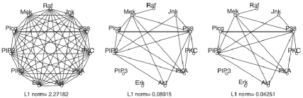
Figure 4: Resulting networks given by graphical lasso algorithm for different values of penalty parameter lambda friedman2008sparse

5 Multiple Hypothesis Testing Problem and False Discovery Rate

We can encounter large scale hypothesis testing problems in many practical situations. For example, in Section 4, we discussed to remove edge from a fully connected graph, we need to perform $p(p-1)/2$ testing problems- $H_{ij}:\!\rho_{ij}=0$ vs $K_{ij}:\!\rho_{ij}\neq 0$. A detailed review can be found in drton2007multiple .

Suppose we have $N$ independent hypothesis $H_{1},\thinspace H_{2},...,\thinspace H_{N}$ to test. In such situations it is important to control not only the type I error of individual hypothesis tests but also the overall (or combined) error rate. It is due to the fact that the probability of atleast one true hypothesis would be rejected becomes large: $1-(1-\alpha)^{N}$, where $\alpha$ being the level of significance, generally taken as 0.05 or 0.01. The conventional way to resolve this problem is by controlling the familywise error rate (FWER)- $P(\cup_{i=1}^{N}H_{0i}\text{ is rejected when it is true$)$}$. One example of such is Bonferroni correction. The problem with this procedure is that it is overly conservative and as a consequence the power of the test will be small. A much more liberal and efficient method for high dimension has been proposed by Benjamini and Hochberg benjamini1995controlling . In figure 5, out of $N$ hypothesis tests in $N_{0}$ cases null hypothesis is true and in $N_{1}$cases null hypothesis is false. According the decision rule, in $R$ out of $N$ cases null hypothesis is rejected. Clearly $R$ is observed but $N_{0}$ or $N_{1}$are not. The following algorithm controls the expected false discovery proportion:

1. The test statistic of $H_{1},\thinspace H_{2},...,\thinspace H_{N}$ yield $p$values $p_{1},.....,p_{N}$ .

2. Order the $p$ values $p_{(1)},.....,p_{(N)}$.

3. Rank the hypothesis $H_{1},\thinspace H_{2},...,\thinspace H_{N}$ according to the $p$values

4. Find largest $j$, say $j^{*}$, such that $p_{j}\leq\frac{j}{N}\alpha$

5. Reject the top $j^{*}$tests as significant.

It can be shown that if the $p$ values are independent of each other then the rule based on the algorithm controls the expected false discovery proportion by $\alpha$, more precisely, $E(\nicefrac{{a}}{{R}})\leq\frac{N_{0}}{N}\alpha\leq\alpha$.

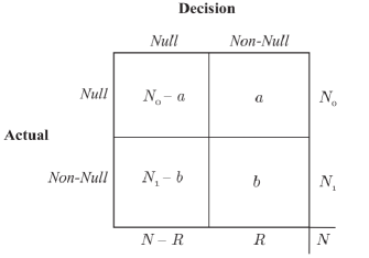
Figure 5: False discovery rate $\nicefrac{{a}}{{R}}$ efron2012large

6 High Dimensional Regression

In financial econometrics one can often encounter multiple regression analysis problem. A large number of predictors implies large number of parameters to be estimated which reduces the degrees of freedom. As a result prediction error will be increased. So in high dimensional regression regularization is an essential tool.

In this section we will breifly discuss the multivariate regression problem with $q$ responses and $p$ predictors, which requires estimation of $pq$ parameters in the regression coefficient matrix. Suppose the matrix of regressors, responses and coefficient matrix are $X$, $Y$ and $B$ respectively. As we know $\hat{B}_{OLS}=(X^{\prime}X)^{-1}X^{\prime}Y$ (under multivariate mormality, this is also the maximum likelihood estimator) with $pq$ parameters. Estimated covariance matrix (with $q(q+1)/2$ parameters) of $Y$ is $\hat{\Sigma}=\frac{1}{n}(Y-X\hat{B})^{\prime}(Y-X\hat{B})$. When $p$ and $q$ are large then both these estimators exhibits poor statistical properties. So here again, shrinkage and regularization of $\hat{B}$ would help to obtain a better estimator. It can be achieved through Reduced Rank Regression which attempts to solve a constrained least square problem:

$$\hat{B}_{r}=\underset{B:\ \mathrm{rank}(B)=r\leq\mathrm{min}(p,q)}{\mathrm{argmin}}tr[(Y-XB)^{\prime}(Y-XB)]$$

The solution of this constrained optimization is $\hat{B}_{r}=(X^{\prime}X)^{-1}X^{\prime}YHH^{\prime}$ where $H=(h_{1},....,h_{r})$ with $h_{k}$ being normalized eigenvector corresponding to the $k$th largest eigenvalue of the matrix $Y^{\prime}X(X^{\prime}X)^{-1}X^{\prime}Y$. Choice of $r$ is important because this is the parameter that balances between bias and variance of prediction.

Alternatively, a regularized estimator can be obtained by introducing a nonnegative penalty function in the optimization problem:

$$\hat{B}=\mathrm{argmin_{B}}\{tr[(Y-XB)^{\prime}(Y-XB)]+\lambda C(B)\}$$

when $C$ is a scalar function and $\lambda$ is nonnegative quantity. Most common choices of $C(B)$ are $l_{p}$ norms. $C(B)=\sum_{j,k}|b_{jk}|$ leads to lasso estimate where as $C(B)=\sum_{j,k}b_{jk}^{2}$ amount to ridge regression. $C(B)=\alpha\sum_{j,k}|b_{jk}|+\nicefrac{{(1-\alpha)}}{{2}}\sum_{j,k}b_{jk}^{2}$ for $\alpha\in(0,1)$ and $C(B)=\sum_{j,k}|b_{jk}|^{\gamma}$ for $\gamma\in[1,2]$ are called elastic net and bridge regression respectively. Grouped lasso with $C(B)=\sum_{i=1}^{p}(b_{j1}^{2}+...+b_{jq}^{2})^{0,5}$ imposes groupwise penalty on the rows of $B$, which may lead to exclusion of some predictors for all the responses.

All the above mentioned methods regularize the matrix $B$ only while leaving $\Sigma$aside. Although a little more complicated, it is sometimes appropriate to regularize both $B$ and $\Sigma^{-1}$. One way to do that is to adding separate lasso penalty on $B$ and $\Sigma^{-1}$in the negative log likelihood:

$$l(B,\Sigma)=\mathrm{tr}[\frac{1}{n}(Y-XB)\Sigma^{-1}(Y-XB)]-\mathrm{log}|\Sigma^{-1}|+\lambda_{1}\sum_{j^{\prime}\neq j}|\omega_{j^{\prime}j}|+\lambda_{2}\sum_{j,k}|b_{j,k}|$$

where $\lambda_{1}$ and $\lambda_{2}$ are as usual tuning parameter, $B=((b_{jk}))$ and $\Sigma^{-1}=\Omega=((\omega_{j^{\prime},j}))$. This optimization problem is not convex but biconvex. Note that solving the above mentioned optimization problem for $\Omega$ with $B$ fixed at $B_{0}$ reduced to the optimization problem:

$$\hat{\Omega}(B_{0})=\mathrm{argmin_{\Omega}}\{tr(\hat{\Sigma}\Omega)-log|\Omega|+\lambda_{1}\sum_{i\neq j}|\omega_{ij}|\}$$

where $\hat{\Sigma}=\frac{1}{n}(Y-XB_{0})^{\prime}(Y-XB_{0})$. If we fix $\Omega$ at a nonnegative definite $\Omega_{0}$ it will lead to

$$\hat{B}(\Omega_{0})=\mathrm{argmin_{B}}\{tr[\frac{1}{n}(Y-XB_{0})\Omega(Y-XB_{0})^{\prime}]+\lambda_{2}\sum_{j,k}|b_{j,k}|\}$$

It can be shown that the original problem can be solved by using the following algorithm prescribed by rothman2010sparse -

• Fix $\lambda_{1}$ and $\lambda_{2}$, initialize $\hat{B}^{(0)}=0$ and $\hat{\Omega}^{(0)}=\hat{\Omega}(\hat{B}^{(0)})$.

  • Step 1: Compute $\hat{B}^{(m+1)}=\hat{B}(\hat{\Omega}^{(m)})$ by solving

    $$\mathrm{argmin_{B}}\{tr(\frac{1}{n}(Y-XB)\Omega(Y-XB)+\lambda_{2}\sum_{j}\sum_{k}|b_{jk}|\}$$

    by coordinate descent algorithm.

  • Step 2: Compute $\hat{\Omega}^{(m+1)}=\hat{\Omega}(\hat{B}^{(m+1)})$ by solving

    $$\mathrm{argmin_{\Omega}}\{tr(\hat{\Sigma}\Omega)-log|\Omega|+\lambda_{1}\sum_{i\neq j}|\omega_{ij}|\}$$

    by Graphical lasso algorithm.

  • Step 3: If $\sum_{i,j}|\hat{b}_{ij}^{(m+1)}-\hat{b}_{ij}^{(m)}|<\epsilon\sum_{i,j}\hat{b}_{ij}^{R}$ where $((\hat{b}_{ij}^{R}))$ is the Ridge estimator of $B$.

7 Principal Components

In many high dimensional studies estimates of principal component loadings are inconsistent and the eigenvectors consists of too many entries to interpret. In such situation regularising the eigenvectors along with eigenvalues would be preferable. So it is desirable to have loading vectors with only a few nonzero entries. The simplest way to achieve that is through a procedure called SCoTLASS jolliffe2003modified . In this approach a lasso penalty is to be imposed on the PC loadings. So the first PC loading can be obtained by solving the optimization problem:

$$\mathrm{maximize_{v}}vX^{\prime}Xv\ \mathrm{subject\ to}\ ||v||_{2}^{2}\leq 1,\ ||v||_{1}\leq c$$

The next PC can be obtained by imposing extra constraint of orthogonality. Note that this is not a minimization problem and so can be difficult to solve. However the above problem is equivalent to the following one:

$$\mathrm{maximize_{u,v}}u^{\prime}Xv\ \mathrm{subject\ to}\ ||v||_{1}\leq c,\ ||v||_{2}^{2}\leq 1,\ ||u||_{2}^{2}\leq 1$$

The equivalence between the two can be easily verified by using Cauchy Schwartz inequality to $u^{\prime}Xv$ and noting that equality will be achieved for $u=\frac{X^{\prime}v}{||X^{\prime}v||_{2}}$. The optimization problem can be solved by the following algorithm witten2009penalized

• Initialize $v$ to have $l_{2}$ norm 1.

• Iterate until convergence

  • $u\leftarrow\frac{Xv}{||Xv||_{2}}$

  • $v\leftarrow\frac{s(X^{\prime}u,\Delta)}{||s(X^{\prime}u,\Delta)||_{2}}$, where $S$ is a soft thresholding operator, and $\Delta=0$ if the computed $v$ satisfies $||v||_{1}\leq c;$ otherwise $\Delta>0$ with $||v||_{1}=c$

8 Classification

Suppose there are $n$ independent observations of training data ($\textbf{X}_{i},\ Y_{i}$), $i=1(1)n$, coming from an unknown distribution. Here $Y_{i}$ denotes the class of the $i$th observation and therefore can take values $\{1,2,3,...,K\}$ if there are $K$ classes. $\textbf{X }_{i}$ , generally a vector of dimension $p$, is the feature vector for the ith observation. Given a new observation X, the task is to determine the class, the observation belongs to. In other words we have to determine a function from the feature space to $\{1,2,...,K\}$. One very widely used class of classifiers is distance based classifiers. It assigns an observation to a class $k$, if the observation is closer to class $k$ on average compared to other classes i.e. $k=\mathrm{argmin_{i}\thinspace dist}(\textbf{X},\mu_{i})$, where $\mu_{i}$ is the center of the feature space of class $i$ . As an example if there are two classes and the feature distribution for the first class is $\textbf{X }\sim N(\mu_{1},\Sigma)$ and for the second class is $\textbf{X}\sim N(\mu_{2},\Sigma)$ then under the assumption that both the classes have equal prior probabilities, the most widely used distance measure is called Mahalanobis’s distance

$$dist(X,\mu_{k})=\sqrt{(X-\mu_{k})\Sigma^{-1}(X-\mu_{k})},k=1,2$$

. So class 1 is to be chosen when

$$\sqrt{(X-\mu_{1})\Sigma^{-1}(X-\mu_{1})}\leq\sqrt{(X-\mu_{2})\Sigma^{-1}(X-\mu_{2})}$$

This technique is called Fisher Discriminant Analysis. For high dimensional data Fisher Discriminant Analysis does not perform well because it involves accurate estimation of precision matrix bickel2004some . In the following section we will discuss some high dimensional classification methods.

8.1 Naive Bayes Classifier

Suppose we classify the observation, with feature x, by some predetermined function $\delta$ i.e. $\delta(\textbf{x})\in\{1,2,..,K\}$. Now to judge the accuracy we need to consider some Loss function. A most intuitive loss function is the zero-one loss: $L(\delta(\textbf{x}),Y)=I(\delta(\textbf{x})\neq Y$), where $I(.)$ is the indicator function. Risk of $\delta$ is the expected loss- $E(L(\delta(\textbf{x}),Y))=1-P(Y=\delta(\textbf{x})|\textbf{X}=\textbf{x})$. The optimal classifier, minimizing the risk, is $g(\textbf{x})=\mathrm{arg\thinspace max_{k}}P(Y=k|\textbf{X}=\textbf{x})$. If $\pi$ be the prior probability of an observation being in class $k$ then by Bayes Theorem $P(Y=k|\textbf{X}=\textbf{x})=\frac{\pi(k)P(\textbf{X}=\textbf{x}|Y=k)}{\sum\pi(k)P(\textbf{X}=\textbf{x}|Y=k)}$. So $g(\textbf{X})=\mathrm{arg\thinspace max_{k}}\pi(k)P(\textbf{X}=\textbf{x}|Y=k)$. This is called Bayes classifier. When X is high dimensional $P(\textbf{X |}Y)$ is practically impossible to estimate. The Naive Bayes Classifier works by assuming conditional independence: $P(\textbf{X}=\textbf{x}|Y=k)=\prod_{i}P(X_{i}=x_{i}|Y=k)$ where $X_{j}$ is the $j$th component of X. Naive Bayes classifier is used in practice even when the conditional independent assumption is not valid. In case of the previous example, under some conditions Naive Bayes classifier outperforms Fisher Discriminant function as long as dimensionality $p$ does not grow faster than sample size $n$.

8.2 Centroid Rule and k-Nearest-Neighbour Rule

The centroid rule classifies an observation to $k$th class if its distance to the centroid of $k$th class is less than that to the centroid of any other class. The merit of this method is illustrated for $K=2$. Suppose $n_{1}$and $n_{2}$ are fixed and $p\rightarrow\infty$ and within each class observations are iid. The observation of two classes can be denoted by $Z_{1}=(Z_{11},Z_{12},...,Z_{1p})$ and $Z_{2}=(Z_{21},...,Z_{2p})$ respectively. With the assumption that as $p\rightarrow\infty$, $\frac{1}{p}\sum_{i=1}^{p}var(Z_{1i})\rightarrow\sigma^{2}$, $\frac{1}{p}\sum_{i=1}^{p}var(Z_{2i})\rightarrow\tau^{2}$ , $\sigma^{2}/n_{1}>\tau^{2}/n_{2}$ and $\frac{1}{p}\sum_{i=1}^{p}[E(Z_{1i}^{2})-E(Z_{2i}^{2})]\rightarrow\kappa^{2}$ a new observation is correctly classified with probability converging to 1 as $p\rightarrow\infty$ if $\kappa^{2}\geq\nicefrac{{\sigma^{2}}}{{n_{1}}}-\nicefrac{{\tau^{2}}}{{n_{2}}}$hall2005geometric .

The $k$-Nearest Neighbour rule determines the class of a new observations by help of $k$ nearest data points from the training data. The new observation is to be assigned to the class closest to

$$g(\textbf{X})=\frac{1}{k}\sum_{i:\!\textbf{X}_{i}\in N_{k}(\textbf{X})}Y_{i}$$

where $N_{k}(\textbf{x})$ is the set $k$ nearest points around x.

8.3 Support Vector Machine

In Bayes classifier, as we discussed, one tries to minimize $\sum_{i}I(g(X)\neq Y)$, with respect to $g(.)$. But it is difficult to work with as indicator function is neither smooth nor convex. So one can think of using a convex loss function. Support vector machine (SVM) claims to resolve that problem. Suppose for binary classification problem, $Y$ takes -1 and 1 to denote two classes. The SVM replaces zero-one loss by convex hinge loss $H(x)=[1-x]_{+}$ where $[u]_{+}=max\{0,u\}$, the positive part of $u$. The SVM tries to minimize $\sum_{i}H(Y_{i}g(\textbf{X}_{i}))+\lambda J(g)$ with respect to $g$. Here $\lambda$ is a tunning parameter and $J$ is a complexity penalty of $g$. If the minimizer is $\hat{g}$ then the SVM classifier is taken to be $sign(\hat{g})$. $J(.)$ can be taken as $L_{2}$ penalty.

It can be shown that the fuction minimizing $E(H(Yg(\textbf{X}))+\lambda J(g))$ is exactly $sign(P(Y=+1|\textbf{X=}\textbf{x})-\frac{1}{2})$ lin2002support . Infact instead of working with $P(Y|\textbf{X}=\textbf{x})$ as in Bayes classifier SVM directly tries to estimate the decision boundary $\{\textbf{x}:\ P(Y=1|\textbf{X}=\textbf{x})=\frac{1}{2}\}$.

8.4 AdaBoost

Among the recently developed methodologies one of the most important is Boosting. It is a method that combines a number of ’weak’ classifiers to form a powerful ’committee’. AdaBoost is the most commonly used boosting algorithm. An interesting result of this algorithm is that it is immuned to overfitting i.e. the test error decreases consistently as more and more classifiers are added. Suppose we have two classes represented as $-1$ and $1$ and denoted by $y$. We have $n$ training data points $(x_{1},y_{1}),\ ,(x_{2},y_{2}),\ ,...,(x_{n},y_{n}).$ We want to produce a committee $F(x)=\sum_{i=1}^{M}c_{m}f_{m}(x)$ where $f_{m}$ is a weak classofier (with values either $1$ or $-1$) that predicts better than random guess. The initial classifiers $f_{m}$ are trained on an weighted version of training sample giving more weight to the cases that are currently misclassified. The ultimate prediction will be based on $sign(F(x))$. This following algorithm is called discrete AdaBoost (as the initial classifier can take only two discrete values +1 and -1) friedman2000additive .

Discrete AdaBoost algorithm:

1. Start with weights $w_{i}=\nicefrac{{1}}{{n}}$ for $i=1(1)n$

2. Repeat for $m=1(1)M$:

   1. Fit the classifier $f_{m}(x)\in\{-1,1\}$ with weights $w_{i}$ on training data.

   2. Compute error $e_{m}=E_{w}[I_{(y\neq f_{m}(x))}]$, where $E_{w}$ is the expectation over the training data with weights $w=(w_{1,}w_{2},...,w_{n})$ and $I(.)$ is an indicator function.

   3. $c_{m}=log(\frac{1-e_{m}}{e_{m}})$

   4. Set $w_{i}\leftarrow w_{i}exp[c_{m}I_{(y_{i}\neq f_{m}(x_{i}))}]$ for $i=1,2,..,n$ and then renormalize to get $\sum_{i}w_{i}=1$.

3. Final classifier: $sign(\sum_{m=1}^{M}c_{m}f_{m}(x))$

The base classifier ($f_{m}(.)$) of Discrete AdaBoost algorithm is binary. It can be generalized further to obtain a modification over discrete AdaBoost algorithm.

Real AdaBoost algorithm:

1. Start with weights $w_{i}=\nicefrac{{1}}{{n}}$ for $i=1(1)n$.

2. Repeat for $m=1(1)M$:

   1. Fit the classifier to obtain the class probability estimate $p_{m}(x)=\hat{P}_{w}(y=1|x)\in[0,1]$, with weights $w=(w_{1},w_{2},...,w_{n})$ on the training data.

   2. Set $f_{m}(x)\leftarrow\frac{1}{2}log\thinspace(p_{m}(x)/(1-p_{m}(x)))\in\mathbf{R}$.

   3. Set $w_{i}\leftarrow w_{i}exp[-y_{i}f_{m}(x_{i})]$, $i=1,2,..,n$ and renormalize so that $\sum_{i}w_{i}=1$.

3. Finale classifier $sign[\sum_{m}f_{m}(x)]$.

It can be shown that AdaBoost method of classification is equivalent to fiiting an additive logistic regression model in a forward stagewise manner friedman2000additive .

Concluding remarks

With the availability of high dimensional economic and financial data many classical statistical methods do not perform well. We have discussed some of the commonly encounted problems related to inference for high dimensional financial data. In many of the approaches signicant improvement can be achieved by bias variance trade off. Some feasible solutions to the problems and some efficient algorithms are discussed. It is to be noted that there are many other challeges related to high dimensional data. Some solutions have been proposed based on simulation studies without desired theoretical justifications.

References

- [1] Yoav Benjamini and Yosef Hochberg. Controlling the false discovery rate: a practical and powerful approach to multiple testing. Journal of the royal statistical society. Series B (Methodological), pages 289–300, 1995.
- [2] Peter J Bickel, Elizaveta Levina, et al. Some theory for fisher’s linear discriminant function,naive bayes’, and some alternatives when there are many more variables than observations. Bernoulli, 10(6):989–1010, 2004.
- [3] Peter J Bickel, Elizaveta Levina, et al. Covariance regularization by thresholding. The Annals of Statistics, 36(6):2577–2604, 2008.
- [4] Vladimir Boginski, Sergiy Butenko, and Panos M Pardalos. Statistical analysis of financial networks. Computational statistics & data analysis, 48(2):431–443, 2005.
- [5] Tony Cai and Weidong Liu. Adaptive thresholding for sparse covariance matrix estimation. Journal of the American Statistical Association, 106(494):672–684, 2011.
- [6] Gary Chamberlain and Michael Rothschild. Arbitrage, factor structure, and mean-variance analysis on large asset markets, 1982.
- [7] Yilun Chen, Ami Wiesel, and Alfred O Hero. Shrinkage estimation of high dimensional covariance matrices. In Acoustics, Speech and Signal Processing, 2009. ICASSP 2009. IEEE International Conference on, pages 2937–2940. IEEE, 2009.
- [8] Arthur P Dempster. Covariance selection. Biometrics, pages 157–175, 1972.
- [9] Mathias Drton and Michael D Perlman. Multiple testing and error control in gaussian graphical model selection. Statistical Science, pages 430–449, 2007.
- [10] Bradley Efron. Large-scale inference: empirical Bayes methods for estimation, testing, and prediction, volume 1. Cambridge University Press, 2012.
- [11] Thomas J Fisher and Xiaoqian Sun. Improved stein-type shrinkage estimators for the high-dimensional multivariate normal covariance matrix. Computational Statistics & Data Analysis, 55(5):1909–1918, 2011.
- [12] Jerome Friedman, Trevor Hastie, and Robert Tibshirani. Sparse inverse covariance estimation with the graphical lasso. Biostatistics, 9(3):432–441, 2008.
- [13] Jerome Friedman, Trevor Hastie, Robert Tibshirani, et al. Additive logistic regression: a statistical view of boosting (with discussion and a rejoinder by the authors). The annals of statistics, 28(2):337–407, 2000.
- [14] LR Haff. Empirical bayes estimation of the multivariate normal covariance matrix. The Annals of Statistics, pages 586–597, 1980.
- [15] Peter Hall, James Stephen Marron, and Amnon Neeman. Geometric representation of high dimension, low sample size data. Journal of the Royal Statistical Society: Series B (Statistical Methodology), 67(3):427–444, 2005.
- [16] Ian T Jolliffe, Nickolay T Trendafilov, and Mudassir Uddin. A modified principal component technique based on the lasso. Journal of computational and Graphical Statistics, 12(3):531–547, 2003.
- [17] Olivier Ledoit and Michael Wolf. A well-conditioned estimator for large-dimensional covariance matrices. Journal of multivariate analysis, 88(2):365–411, 2004.
- [18] Shang P Lin. A monte carlo comparison of four estimators for a covariance matrix. Multivariate Analysis, 6:411–429, 1985.
- [19] Yi Lin. Support vector machines and the bayes rule in classification. Data Mining and Knowledge Discovery, 6(3):259–275, 2002.
- [20] Brett Naul, Bala Rajaratnam, and Dario Vincenzi. The role of the isotonizing algorithm in stein’s covariance matrix estimator. Computational Statistics, 31(4):1453–1476, 2016.
- [21] Theophilos Papadimitriou, Periklis Gogas, and Georgios Antonios Sarantitis. European business cycle synchronization: A complex network perspective. In Network Models in Economics and Finance, pages 265–275. Springer, 2014.
- [22] Mohsen Pourahmadi. High-dimensional covariance estimation: with high-dimensional data, volume 882. John Wiley & Sons, 2013.
- [23] Adam J Rothman. Positive definite estimators of large covariance matrices. Biometrika, 99(3):733–740, 2012.
- [24] Adam J Rothman, Elizaveta Levina, and Ji Zhu. Sparse multivariate regression with covariance estimation. Journal of Computational and Graphical Statistics, 19(4):947–962, 2010.
- [25] Juliane Schäfer and Korbinian Strimmer. A shrinkage approach to large-scale covariance matrix estimation and implications for functional genomics. Statistical applications in genetics and molecular biology, 4(1), 2005.
- [26] Charles Stein. Inadmissibility of the usual estimator for the mean of a multivariate normal distribution. Technical report, STANFORD UNIVERSITY STANFORD United States, 1956.
- [27] Charles Stein. Estimation of a covariance matrix, rietz lecture. In 39th Annual Meeting IMS, Atlanta, GA, 1975, 1975.
- [28] Charles Stein et al. Inadmissibility of the usual estimator for the mean of a multivariate normal distribution. In Proceedings of the Third Berkeley symposium on mathematical statistics and probability, volume 1, pages 197–206, 1956.
- [29] N Vandewalle, F Brisbois, X Tordoir, et al. Non-random topology of stock markets. Quantitative Finance, 1(3):372–374, 2001.
- [30] Daniela M Witten, Robert Tibshirani, and Trevor Hastie. A penalized matrix decomposition, with applications to sparse principal components and canonical correlation analysis. Biostatistics, 10(3):515–534, 2009.
- [31] Lingzhou Xue, Shiqian Ma, and Hui Zou. Positive-definite 1-penalized estimation of large covariance matrices. Journal of the American Statistical Association, 107(500):1480–1491, 2012.
- [32] Ming Yuan and Yi Lin. Model selection and estimation in the gaussian graphical model. Biometrika, 94(1):19–35, 2007.