Nearby high-speed stars in Gaia DR2

Abstract

We investigate the nature of nearby (10–15 kpc) high-speed stars in the Gaia DR2 archive identified on the basis of parallax, proper motion and radial velocity. Together with a consideration of their kinematic, orbital, and photometric properties, we develop a novel strategy for evaluating whether high speed stars are statistical outliers of the bound population or unbound stars capable of escaping the Galaxy. Out of roughly 1.5 million stars with radial velocities, proper motions, and 5-$\sigma$ parallaxes, we identify just over 100 high-speed stars. Of these, only two have a nearly 100% chance of being unbound, with indication that they are not just bound outliers; both are likely hyper-runaway stars. The rest of the high speed stars are likely statistical outliers. We use the sample of high-speed stars to demonstrate that radial velocity alone provides a poor discriminant of nearby, unbound stars. However, these stars are efficiently identified from the tangential velocity, using just parallax and proper motion. Within the full Gaia DR2 archive of stars with 5-$\sigma$ parallax and proper motion but no radial velocity, we identify a sample of 19 with speeds significantly larger than the local escape speed of the Milky Way based on tangential motion alone.

1 INTRODUCTION

The recent release of the Gaia DR2 catalog (Gaia Collaboration et al., 2018a) has renewed interest in the highest velocity stars in the Galaxy. In addition to contributing new samples of candidates (e.g., Marchetti et al., 2018b; Shen et al., 2018; Hattori et al., 2018a), Gaia proper motions and radial velocities allow more robust assessments of the distances and space velocities of previously identified high velocity stars (e.g., Boubert et al., 2018; Brown et al., 2018; Raddi et al., 2018). As a result of these analyses, some stars are clearly unbound. Others are just barely bound to the Milky Way.

The 6-D positions and velocities available for over 7 million sources in the Gaia DR2 archive also enable new tests of theoretical models for the highest velocity stars. In the current paradigm, hyper-runaway stars (HRSs) result from dynamical interactions among groups of massive stars (e.g., Poveda et al., 1967; Leonard, 1991; Perets & Subr, 2012) or the explosion of a massive star in a close binary (e.g., Blaauw, 1961; De Donder et al., 1997; Portegies Zwart, 2000; Perets & Subr, 2012). The supermassive black hole in the Galactic Center may also disrupt a close binary system, capture one component, and eject the other as a hypervelocity star (HVS; Hills, 1988; Yu & Tremaine, 2003). Other physical mechanisms may also accelerate stars to high velocity (e.g., Sesana et al., 2006; Yu & Madau, 2007; Sesana et al., 2009; Abadi et al., 2009; Piffl et al., 2014; Capuzzo-Dolcetta & Fragione, 2015; Fragione & Capuzzo-Dolcetta, 2016; Subr & Haas, 2016; Hamers & Perets, 2017). Comparisons between observed and predicted space motions yield constraints on the Galactic potential and the ejection mechanism (e.g., Bromley et al., 2006; Kenyon et al., 2008; Bromley et al., 2009; Kenyon et al., 2014; Rossi et al., 2014, 2017; Hattori et al., 2018b; Marchetti et al., 2018a; Kenyon et al., 2018).

Here, we use the Gaia DR2 proper motion and radial velocity data for the brightest stars to test several aspects of theoretical models for HRSs and HVSs (see also Marchetti et al., 2018a, b). Based on existing samples of HVSs with B-type spectra in the outer halo (e.g., Brown et al., 2005; Edelmann et al., 2005; Hirsch et al., 2005; Brown et al., 2006a, b, 2007a, 2007b, 2009, 2012, 2013, 2014, 2015; Brown, 2015), the probability of detecting more than one B-type HVS within 10 kpc of the Sun is small (Kenyon et al., 2008, 2014). Finding nearby HRSs is much easier (Bromley et al., 2009; Kenyon et al., 2014). For either HRSs or HVSs, surveys using the Galactic rest-frame tangential velocity should return a higher proportion of nearby high velocity stars than the radial velocity (Kenyon et al., 2018). Our goal is to test these predictions with Gaia data.

Identifying true high-velocity outliers in the Gaia DR2 archive is challenging. Among the roughly 7 million stars with measured parallax, proper motion, and radial velocity, no more than a few hundred candidates emerge with Galactic rest-frame velocity close to or exceeding the local escape velocity (e.g., Marchetti et al., 2018b; Hattori et al., 2018a). Based on the quoted errors of the measured quantities, only a few outliers unambiguously exceed the escape velocity. Our goal is to consider the wealth of kinematic information available in the Gaia data to analyze the distribution of dynamical parameters and their errors and to make robust estimates of the number of true outliers in the velocity distribution.

Aside from identifying potential HRSs or HVSs, our analysis is important for measuring the local escape velocity and the mass of the Milky Way (e.g., Patel et al., 2018; Gaia Collaboration et al., 2018c; Watkins et al., 2018; Posti & Helmi, 2018; Monari et al., 2018). All of the Gaia stars with radial velocity data lie within roughly 15 kpc of the Sun. Understanding which of these stars have velocities smaller than the local escape velocity helps to establish the mass of the Milky Way within 20 kpc of the Galactic Center (see also Monari et al., 2018). Our analysis provides a strategy to isolate unbound outliers from those bound to the Milky Way.

We begin with a discussion of the sample selection in §2 and the basic properties of candidate high velocity stars in §3. In §4, we assess the effectiveness of using radial velocities and proper motion separately to identify high-speed sources, and in §5 we introduce a new set of candidate stars selected on the basis of proper motion only. Comparisons with theory follow in §6. We conclude with a brief summary in §7.

2 SAMPLE SELECTION

We select stars with well-constrained position and velocity vectors, seeking sources with measurements of radial velocity $v_{\text{r}}$, parallax $\varpi$, and proper motion $\vec{\mu}=(\mu_{\alpha},\mu_{\delta})$, where the vector components are along right ascension $\alpha$ and declination $\delta$, respectively. The Gaia DR2 archive (Gaia Collaboration et al., 2016) lists 7,224,631 stars with estimates of all of these parameters. This section describes our astrometric selection of these “6-D” stars, distance estimation and a novel numerical approach to it, and the measurement of source parameters in the Galactic rest frame.

Nearly all stars with high-quality astrometry and radial velocity data are bound to the Galaxy. Defining $p_{\text{unb}}$ as the probability a star is unbound, we seek stars with a 3-$\sigma$ confidence level $p_{\text{unb}}\geq$ 0.997. To construct a reasonable set of outliers, we identify groups of stars with $p_{\text{unb}}\geq$ 0.2 and $p_{\text{unb}}\geq$ 0.5 (see also Marchetti et al., 2018b; Hattori et al., 2018a). In §4, we develop a new approach to quantify this probability based on a consideration of the error distribution for the large population of bound stars. This method enables us to determine whether an unbound candidate has measured kinematical properties that stand out from the bound outliers. A handful of the highest-speed stars emerge as promising.

2.1 Astrometric selection criteria

To select stars with high-quality astrometry, we follow the recommendations in the basic source parameter descriptions (Gaia Collaboration et al., 2018b) by requiring

$$\texttt{astrometric\_gof\_al}<3, \texttt{astrometric\_excess\_noise}\leq 2,$$

$$-0.23< \texttt{mean\_varpi\_factor\_al}\leq 0.32, \texttt{visibility\_periods\_used}>9.$$

We also make cuts based on photometry that impact the quality of the astrometry:

$$1+0.015\times(\texttt{bp\_rp})^{2}<\texttt{phot\_bp\_rp\_excess\_factor}<1.3+0.06\times(\texttt{bp\_rp})^{2}$$

$$\chi_{\nu}^{2}<1.2\times\max\{1.0,\exp[-0.2*(\texttt{phot\_g\_mean\_mag}-19.5)]\}$$

$$\chi_{\nu}^{2}\equiv\texttt{astrometric\_chi2\_al}/(\texttt{astrometric\_n\_good\_obs\_al}-5)$$

(see Lindegren et al., 2018, Equations C.1 and C.2, therein). In addition, we admit only those sources that have

$$\texttt{rv\_nb\_transits}>5,$$

a condition that provides assurance of the quality of the reported radial velocity, indicating that $v_{\text{r}}$ measurements were taking at a minimum of six distinct epochs. This step helps to eliminate confusion from binary stars. Applying all of these criteria yields 1,519,451 stars.

The basic source parameter, duplicated_source, indicates possibly compromised astrometry for stars in crowded fields (Gaia Collaboration et al., 2018b). We accept stars even when this flag is raised (about 13% of the roughly $1.5\times 10^{6}$ objects) to enable comparisons with previous results that do not use this selection criterion (see Marchetti et al., 2018b; Hattori et al., 2018a). For the high-speed objects of primary interest, this flag is raised once in a set of 25 objects.

Here, we include only stars with median parallax $\varpi>0$ and relative error $\sigma_{\varpi}/\varpi<0.2$, corresponding to a 5-$\sigma$ detection. This threshold enables a straightforward estimate of distance from the inverse of the parallax (e.g., Bailer-Jones, 2015, although see Luri et al. 2018 and our next discussion). It is also restrictive enough to provide meaningful estimates of whether sources are unbound to the Galaxy, yet it eliminates fewer than 3% of the sources that survive the Gaia-recommended quality cuts listed above. The result is a “5-$\sigma$ sample” of $N_{\textit{s}}=$1,475,207 stars.

2.2 Distance estimates from Gaia parallaxes

A first step in assessing how sources in our sample are traveling with respect to the Galaxy is the transformation of basic archive data into physical distances and speeds. A key element in the process is the inference of heliocentric distance ${d}_{\text{h}}$ from parallax. While the significance of the parallax detections in our 5-$\sigma$ sample is high, parallax errors are not negligible. The parallax error distribution of Gaia DR2 sources is well-approximated by a Gaussian (Lindegren et al., 2018), with a tail formally extending to unphysical, negative values. When converting to distance using the inversion formula ${d}_{\text{h}}=1/\varpi$, even small values allowed by the uncertainties may be unrealistic, based on the understanding that the source is a star in the Milky Way.

A way to mitigate the problem is to select only sources that have small relative parallax errors (e.g., Hattori et al., 2018a). When the parallax error distribution is narrow compared to the measured parallax, the extreme tails of the distribution are negligible. Then the inverse of the median parallax gives a reliable distance estimate, ${d}_{\text{h}}=1/\varpi$. Inverted samples of the parallax error distribution also give a good representative set of possible distance measurements.

A more general approach, Bayesian inference, incorporates prior information about source locations (e.g., Bailer-Jones, 2015; Astraatmadja & Bailer-Jones, 2016; Luri et al., 2018). From Bayes’ Theorem, the posterior distribution of distances, $P({d}_{\text{h}}|\varpi,\sigma_{\varpi})$, given a measured parallax $\varpi$ with uncertainty $\sigma_{\varpi}$, is

$$P_{\text{post}}({d}_{\text{h}}|\varpi,\sigma_{\varpi})\sim P_{\text{cond}}(\varpi|{d}_{\text{h}},\sigma_{\varpi})P_{\text{prior}}({d}_{\text{h}}),$$ (1)

where $P_{\text{cond}}(\varpi|{d}_{\text{h}},\sigma_{\varpi})$ is the distribution of parallax values given a distance ${d}_{\text{h}}$ (here, a Gaussian with mean $1/{d}_{\text{h}}$), and $P_{\text{prior}}({d}_{\text{h}})$ is the prior distribution that contains assumptions about where a source is located. Bailer-Jones (2015) introduces

$$P_{\text{prior}}\sim{d}_{\text{h}}^{2}\exp(-{d}_{\text{h}}/L),$$ (2)

corresponding to an exponential fall-off in density, with a most probable source location at $2L$. Marchetti et al. (2017) set $L=2.6$ kpc to represent bulk of the Gaia stars, averaged over the plane of the sky. Bailer-Jones et al. (2018) adopt values around 1 kpc, depending on the sky location relative to the Galaxy. However, we hesitate to adopt priors that are tailored to the bulk catalog in a search for rare, unbound stars on orbits that are not known a priori.

When the parallax uncertainty is large compared to the measured parallax, Bayesian distance estimates are dominated by the choice of prior. When the relative parallax errors are small, reasonable priors have little influence on the inferred distance. Our threshold, $\sigma_{\varpi}/\varpi=0.2$, is on the boundary between these two cases (e.g., Bailer-Jones, 2015; Astraatmadja & Bailer-Jones, 2016). For a 5-$\sigma$ detection, nearly all parallaxes consistent with measurement of a source correspond to physical distances, enabling a blind search for rare, unknown sources. Furthermore, the 5-$\sigma$ sample is not strongly affected by potential systematic errors in parallax (Lindegren et al., 2018). Nonetheless, priors as in equation (2) may modestly affect the noisier sources in the our sample (cf. Marchetti et al., 2018b). Thus, we perform our analysis with and without priors to understand their impact. Our analysis demonstrates that our most promising high-speed sources and our overall conclusions are not affected by this choice.

2.3 Galactocentric quantities

Our analysis of the 5-$\sigma$ sample requires estimates of a source’s position and velocity relative to the Galactic Center. To obtain these quantities, we assume that the Sun has a position vector $(X_{\odot},Y_{\odot},Z_{\odot})=(-8,0,0)$ kpc and a velocity vector $(U_{\odot},V_{\odot},W_{\odot})=(11.1,247.24,7.25)$ km/s (e.g., Schönrich et al., 2010) in a right-handed coordinate system ($X,Y,Z,U,V,W$) where the origin is fixed at the Galactic Center (e.g., Johnson & Soderblom, 1987). The Sun’s velocity includes a contribution of $V=235$ km/s from the rotation of the Galactic disk (e.g. Reid et al., 2014). These definitions allow us to transform Gaia measurements into the Galactic frame of reference.

To estimate Galactocentric position, velocity, and derived quantities from the parallax, proper motion, and radial velocity, we account for uncertainties and correlations between measurements as specified in Gaia DR2 basic source parameter list. We group together the measured quantities as a vector,

$${\vec{{{\xi}}}}=\{{{\xi}}_{i}\}\equiv(\varpi,\mu_{\alpha},\mu_{\delta},v_{\text{r}}),$$ (3)

and, with index $i$ running from one to four, write the elements of the corresponding covariance matrix,

$${\cal C}_{ii}=\sigma_{i}^{2}\text{\ \ and\ \ }{\cal C}_{ij}=\sigma_{i}\sigma_{j}\rho_{ij}\ \ (i\neq j),$$ (4)

where $\sigma_{i}$ is the uncertainty in ${{\xi}}_{i}$, and $\rho_{ij}$ is the correlation coefficient for measurements ${{\xi}}_{i}$ and ${{\xi}}_{j}$. The Gaia DR2 archive lists all of the uncertainties and correlation coefficients, except that radial velocity is uncorrelated with parallax and proper motion, so $\rho_{i<4,4}=0$.

We take a Monte Carlo approach to error estimation, generating samples from the joint distribution of parallax, proper motion and radial velocity, as specified by the measured median values, uncertainties and correlations. In our “Quasi-Monte Carlo” implementation, low-discrepancy sequences form realizations of quasi-random 4-vectors, uniformly distributed in the unit hypercube (Sobol, 1976; Press et al., 1992). A pair of 2-D Box-Muller transformations converts each quasi-random vector into a new 4-vector $\vec{n}$, whose components are (quasi-)independent and normally distributed. A Cholesky factorization of the covariance matrix ${\cal C}$ in equation (4) transforms this vector into the Gaia observables, ${\vec{{{\xi}}}}={\cal C}^{1/2}\vec{n}$. In this way, we generate $N=4,096$ realizations of $(\varpi,\mu_{\alpha},\mu_{\delta},v_{\text{r}})$ per star. If heliocentric distance estimates come from $1/\varpi$, then samples are converted geometrically into desired quantities like Galactocentric distance (${r}_{\text{g}}$) and speed (${v}_{\text{g}}$).

When heliocentric distance ${d}_{\text{h}}$ comes from Bayesian estimation, the Quasi-Monte Carlo procedure just described is modified to sample a 4-D distribution with ${d}_{\text{h}}$ replacing parallax as a variate, distributed according to the posterior, $P_{\text{post}}$. To maintain correlations with proper motion samples, practitioners recommend Markov Chain Monte Carlo (MCMC) methods (e.g., Marchetti et al., 2017; Luri et al., 2018). Because the distance priors considered here are proper and functions of ${d}_{\text{h}}$ alone, we instead calculate the cumulative posterior distribution, $P_{\text{post}}(<{d}_{\text{h}})$, and numerically invert it. The $i$-th sample of a uniform variate $u$ then yields distance ${d}_{\text{h,i}}=P_{\text{post}}^{-1}(u_{i})$. To preserve correlations between ${d}_{\text{h,i}}$ and proper motion, we generate Quasi-Monte Carlo trials as before but in the transformation of the $i$-th set of independent normal quasi-random variates to observables, ${\vec{{{\xi}}}}_{i}={\cal C}^{1/2}\vec{n}_{i}$, we make the substitution

$$n_{1,i}\rightarrow(1/{d}_{\text{h,i}}-\varpi)/\sigma_{\varpi}\ \ \ \ ({d}_{\text{h,i}}>0).$$ (5)

This step takes advantage of the lower triangular form of ${\cal C}^{1/2}$ from the Cholesky factorization. As a check, we reproduce results obtained with a full 4-D MCMC solver from the emcee package (Foreman-Mackey et al., 2013).

Compared to MCMC, and to pseudorandom methods generally, the Quasi-Monte Carlo approach converges quickly, like a grid-based integrator (e.g., Press et al., 1992). For example, with $N=4,096$, estimates of ${\sigma}_{v,\text{g}}$, the 1-$\sigma$ error in Galactocentric speed, are typically accurate to within a few tenths of a percent. Pseudorandom Monte Carlo trials with the same $N$ yield estimates with uncertainties of a few percent. The MCMC approach also gives errors of several percent with that same number of trials, not including the “burn-in” steps (Foreman-Mackey et al., 2013).

2.4 Orbit selection: bound versus unbound

Next we identify high-speed stars that are potentially on unbound orbits relative to the Galaxy. We use the Galaxy model composed of a compact bulge, a rotating disk, and an extended, dark matter halo described in Kenyon et al. (2014, 2018). The Galactic potential $\Phi$ is the sum of the potential of each component; the model parameters (Kenyon et al., 2018, §3.1 therein) are consistent with recent Gaia observations of the mass of the Milky Way (cf. Callingham et al., 2018; Fritz et al., 2018; Watkins et al., 2018).

From the gravitational potential, we obtain a local escape speed, ${v}_{\text{esc}}(\vec{r}_{\text{g}})$, defined as the minimum speed of a star that reaches a distance of 250 kpc from the Galactic Center:

$${v}_{\text{esc}}=\sqrt{2[\Phi(\vec{r}_{250})-\Phi(\vec{r}_{\text{g}})]}.$$ (6)

For simplicity, we take $\vec{r}_{250}$ as a point at that distance on the symmetry axis of the Galactic disk. An unbound orbit has ${v}_{\text{g}}\geq{v}_{\text{esc}}$. Quasi-Monte Carlo draws of ${r}_{\text{g}}$ and ${v}_{\text{g}}$ from the error distributions of each source give the fraction of trials that yield unbound orbits; this fraction is our estimator for $p_{\text{unb}}$, the probability that a star is unbound.

There are 25 candidate high velocity stars with $p_{\text{unb}}$ exceeding 50%. An additional 101 candidates have a 20% or better likelihood of being on an unbound orbit ($p_{\text{unb}}\geq 0.2$). Table 1 reproduces the Gaia DR2 basic source parameters for the 25 high-speed outliers.

Table 1: High-speed stars: Gaia DR2 basic source parameters

Gaia DR2	($\alpha$, $\delta$)	$\varpi$	$\mu_{\alpha}$	$\mu_{\delta}$	rv	G	$G_{\text{BP}}$	BP-RP
designation	(deg)	(mas)	(mas/yr)	(mas/yr)	(km/s)	(mag)	(mag)	(mag)
5932173855446728064M,d	(244.118100,-54.440452)	0.454$\pm$0.029	-2.68$\pm$0.04	-4.99$\pm$0.03	-614.29$\pm$2.49	13.81	14.21	0.99
1383279090527227264M	(240.337348, 41.166774)	0.118$\pm$0.016	-25.76$\pm$0.03	-9.75$\pm$0.04	-180.90$\pm$2.42	13.01	13.51	1.16
1478837543019912064	(212.477709, 33.712932)	0.105$\pm$0.019	-17.61$\pm$0.02	-16.57$\pm$0.03	-245.88$\pm$1.48	13.09	13.51	1.00
6456587609813249536M	(317.360892,-57.912400)	0.099$\pm$0.019	13.00$\pm$0.03	-18.26$\pm$0.03	-15.85$\pm$2.83	13.01	13.47	1.08
6492391900301222656M	(348.646647,-58.429575)	0.095$\pm$0.018	7.50$\pm$0.03	-15.82$\pm$0.03	-149.86$\pm$1.16	13.36	13.94	1.29
4326973843264734208M	(248.892295,-14.518435)	0.199$\pm$0.031	-20.55$\pm$0.05	-33.97$\pm$0.03	-220.39$\pm$2.05	13.50	14.43	1.87
5846998984508676352	(211.089783,-69.345114)	0.095$\pm$0.019	-16.20$\pm$0.02	-2.69$\pm$0.03	31.43$\pm$4.38	14.14	14.92	1.63
2089995308886282880M	(280.928177, 31.345968)	0.071$\pm$0.013	-3.17$\pm$0.02	-9.50$\pm$0.02	-9.90$\pm$0.52	13.18	13.89	1.51
5802638672467252736M	(255.717030,-74.057467)	0.101$\pm$0.015	-8.72$\pm$0.02	-15.29$\pm$0.02	70.53$\pm$1.46	13.06	13.70	1.39
2095397827987170816M	(276.654116, 35.056068)	0.066$\pm$0.012	-3.13$\pm$0.02	-8.86$\pm$0.02	-96.95$\pm$1.11	13.45	14.15	1.51
6431596947468407552M	(274.687922,-70.249323)	0.084$\pm$0.016	4.55$\pm$0.02	4.97$\pm$0.02	259.08$\pm$1.65	13.09	13.66	1.28
2159020415489897088M	(273.321443, 61.318680)	0.134$\pm$0.026	3.99$\pm$0.05	15.67$\pm$0.05	-162.28$\pm$0.99	12.51	13.12	1.33
5919596571872806272	(265.896592,-56.104065)	0.120$\pm$0.022	-11.03$\pm$0.04	-20.09$\pm$0.04	212.10$\pm$2.21	13.01	13.57	1.28
2121857472227927168M	(275.124461, 47.497863)	0.072$\pm$0.013	-5.36$\pm$0.02	-7.06$\pm$0.02	-434.70$\pm$0.71	13.27	13.96	1.49
5839686407534279808M	(209.437107,-72.149655)	0.138$\pm$0.020	-22.74$\pm$0.03	-3.18$\pm$0.03	175.38$\pm$4.87	13.91	14.84	1.87
2112308930997657728M	(272.894471, 39.889802)	0.167$\pm$0.022	-21.92$\pm$0.04	-12.60$\pm$0.04	-107.02$\pm$1.40	12.58	13.02	1.04
6656557095228727936	(286.480891,-52.679280)	0.105$\pm$0.020	2.31$\pm$0.03	-18.83$\pm$0.02	-85.25$\pm$2.60	13.43	13.94	1.17
5399966178291369728M	(166.880803,-37.647268)	0.100$\pm$0.017	-12.87$\pm$0.02	0.51$\pm$0.02	420.38$\pm$1.84	13.08	13.69	1.36
4366218814874247424M	(256.061406, -2.675249)	0.139$\pm$0.021	-19.29$\pm$0.04	6.03$\pm$0.03	-132.81$\pm$1.22	13.17	13.89	1.54
5217818333256869376M	(141.829543,-73.543300)	0.118$\pm$0.018	-13.27$\pm$0.04	8.27$\pm$0.04	375.09$\pm$1.26	12.48	13.10	1.37
6124121132097402368	(212.016640,-32.476408)	0.120$\pm$0.024	-19.81$\pm$0.04	-2.60$\pm$0.04	85.24$\pm$1.21	13.05	13.61	1.25
2106519830479009920M	(285.484415, 45.971657)	0.123$\pm$0.018	3.30$\pm$0.04	13.17$\pm$0.04	-212.12$\pm$0.98	12.42	13.04	1.35
5835015235520194944	(244.519790,-58.328708)	0.118$\pm$0.020	-16.31$\pm$0.03	-13.74$\pm$0.03	106.78$\pm$1.49	13.17	13.99	1.70
1989862986804105344M	(340.509702, 51.611096)	0.095$\pm$0.016	10.34$\pm$0.02	5.09$\pm$0.02	-75.70$\pm$1.62	13.08	13.72	1.39
5779919841659989120M	(235.357736,-77.283183)	0.094$\pm$0.016	-11.43$\pm$0.03	-8.40$\pm$0.03	-13.31$\pm$0.83	13.55	14.39	1.71

Note. — This list is in order of decreasing probability of being unbound (see Table 2). In the first column, the superscript “d” indicates that the duplicated_source flag is raised, while the “M” indicates that a source is also listed in Marchetti et al. (2018b).

Table 2 lists Galactocentric data for the 25 high-speed outliers, sorted by decreasing probability of being unbound. It includes heliocentric distance (${d}_{\text{h}}$), Galactocentric distance (${r}_{\text{g}}$) and speed (${v}_{\text{g}}$), along with Galactocentric speeds inferred from either the heliocentric radial velocity or proper motion:

$$v_{\text{r,g}} = v_{\text{r}}+\vec{v}_{\odot,\text{g}}\cdot\hat{r},$$ (7)

$$\vec{v}_{\text{pm,g}} = k\frac{\vec{\mu}}{\varpi}+\vec{v}_{\odot,\text{g}}-(\vec{v}_{\odot,\text{g}}\cdot\hat{r})\hat{r},$$ (8)

where $\vec{v}_{\odot,\text{g}}$ is the Sun’s velocity in the Galaxy’s rest frame, and $\hat{r}$ is the unit vector in the direction of the Sun in that frame. Equation (7) gives the observer-frame line-of-sight component of the Galactic velocity, corrected for Solar motion; equation (8) gives the Galactocentric velocity vector in the observer’s sky plane, corrected for Solar motion, as estimated from the parallax and the proper motion vector $\vec{\mu}=(\mu_{\alpha},\mu_{\delta})$ in equatorial coordinates. The constant $k$ in equation (8) has a value of 4.7047 when speed, parallax, and proper motion are in units of km/s  mas, and mas/yr, respectively.

Table 2 also includes $\gamma$, the angle between each star’s radial position and velocity:

$$\cos\gamma=\hat{v}_{\text{g}}\cdot\hat{r}_{\text{g}}=\frac{\vec{r}_{\text{g}}\cdot\vec{v}_{\text{g}}}{|\vec{r}_{\text{g}}||\vec{v}_{\text{g}}|}.$$ (9)

Stars on purely radial, outbound orbits have $\gamma=0^{\circ}$; stars orbiting the Galactic Center have $\gamma=90^{\circ}$. The $L_{\text{Z}}/L_{200}$ parameter, the $Z$-component of the stars’ angular momentum relative to a disk-like orbit with $|\vec{L}_{200}|={r}_{\text{g}}\times 200$ km/s, indicates how stars move relative to the rotation of stars in the Milky Way’s disk. Similarly, the quantity

$${v_{\text{Z}}}/v_{\bot}\equiv\ \frac{W}{\left(U^{2}+V^{2}\right)^{1/2}}$$ (10)

establishes out-of-plane motion as compared with the speed in a plane parallel to the disk. This measure also serves to distinguish disk stars from the halo population.

Table 2: High-stars stars: Galactocentric kinematical parameters.

Gaia DR2	($\ell$,$b$)	${d}_{\text{h}}$	${r}_{\text{g}}$	${v}_{\text{g}}$	$v_{\text{r,g}}$	$v_{\text{t,g}}$	$\gamma$	$L_{\text{Z}}/L_{200}$	${v_{\text{Z}}}/v_{\bot}$	$p_{\text{unb}}$
designation	(deg)	(kpc)	(kpc)	(km/s)	km/s	km/s	(deg)
5932173855446728064	(329.9, -2.7)	2.2$\pm$0.1	6.2$\pm$0.1	747$\pm$3	-728.7$\pm$2.5	164$\pm$4	53.0$\pm$0.6	3.0$\pm$0.0	0.02$\pm$0.00	1.00
1383279090527227264	( 65.5, 48.8)	8.5$\pm$1.3	10.0$\pm$0.9	924$\pm$168	-24.4$\pm$2.4	924$\pm$168	86.7$\pm$0.6	-2.3$\pm$0.3	0.79$\pm$0.01	1.00
1478837543019912064	( 59.0, 71.9)	9.6$\pm$2.1	11.4$\pm$1.6	876$\pm$230	-171.3$\pm$1.5	859$\pm$234	95.9$\pm$0.7	-2.5$\pm$0.5	0.09$\pm$0.04	0.99
6456587609813249536	(338.3,-40.9)	10.1$\pm$2.4	7.3$\pm$1.7	889$\pm$250	-82.0$\pm$2.8	885$\pm$251	51.3$\pm$9.0	0.8$\pm$2.5	-0.33$\pm$0.01	0.98
6492391900301222656	(324.6,-54.4)	10.5$\pm$2.4	9.7$\pm$1.8	678$\pm$189	-233.8$\pm$1.2	637$\pm$198	93.0$\pm$0.4	-0.3$\pm$0.7	0.60$\pm$0.09	0.81
4326973843264734208	( 2.6, 21.5)	5.0$\pm$0.9	3.8$\pm$0.4	730$\pm$159	-197.0$\pm$2.1	703$\pm$164	91.8$\pm$5.3	-3.1$\pm$0.4	-0.24$\pm$0.03	0.79
5846998984508676352	(309.3, -7.4)	10.5$\pm$2.5	8.3$\pm$1.9	671$\pm$189	-152.2$\pm$4.4	654$\pm$193	55.9$\pm$6.9	2.6$\pm$3.9	0.15$\pm$0.01	0.74
2089995308886282880	( 60.7, 15.2)	14.2$\pm$3.2	12.6$\pm$2.8	605$\pm$144	205.3$\pm$0.5	569$\pm$151	104.3$\pm$2.7	2.8$\pm$1.9	-0.07$\pm$0.00	0.73
5802638672467252736	(317.9,-19.1)	9.9$\pm$1.6	7.2$\pm$1.1	648$\pm$135	-80.6$\pm$1.5	643$\pm$136	45.6$\pm$7.8	1.9$\pm$1.2	-0.10$\pm$0.01	0.70
2095397827987170816	( 63.0, 19.9)	15.1$\pm$3.3	13.7$\pm$2.9	585$\pm$142	117.4$\pm$1.1	573$\pm$144	110.3$\pm$3.7	2.5$\pm$1.7	-0.05$\pm$0.01	0.69
6431596947468407552	(324.2,-22.7)	12.0$\pm$2.7	8.0$\pm$2.2	605$\pm$84	131.2$\pm$1.7	591$\pm$85	105.4$\pm$5.7	-1.7$\pm$1.5	-0.44$\pm$0.00	0.66
2159020415489897088	( 90.5, 28.1)	7.5$\pm$1.8	11.0$\pm$1.3	588$\pm$134	59.2$\pm$1.0	585$\pm$135	41.1$\pm$5.4	-1.1$\pm$1.1	-0.25$\pm$0.02	0.65
5919596571872806272	(336.2,-13.5)	8.3$\pm$1.8	3.8$\pm$0.9	684$\pm$188	123.3$\pm$2.2	672$\pm$190	26.8$\pm$8.3	0.2$\pm$2.7	-0.06$\pm$0.01	0.63
2121857472227927168	( 75.5, 24.7)	14.0$\pm$3.0	14.4$\pm$2.6	550$\pm$114	-211.6$\pm$0.7	507$\pm$122	141.8$\pm$8.8	1.1$\pm$1.0	0.07$\pm$0.06	0.62
5839686407534279808	(308.0, -9.9)	7.2$\pm$1.1	6.8$\pm$0.5	626$\pm$123	-11.0$\pm$4.9	625$\pm$123	25.7$\pm$6.7	1.0$\pm$0.8	0.12$\pm$0.00	0.62
2112308930997657728	( 67.0, 24.2)	6.0$\pm$0.8	8.1$\pm$0.4	601$\pm$100	107.4$\pm$1.4	592$\pm$101	118.0$\pm$1.5	0.3$\pm$0.2	0.96$\pm$0.02	0.62
6656557095228727936	(344.2,-23.4)	9.5$\pm$2.1	4.5$\pm$1.5	661$\pm$187	-140.2$\pm$2.6	646$\pm$190	50.7$\pm$13.3	1.3$\pm$2.9	-0.41$\pm$0.01	0.62
5399966178291369728	(281.2, 20.8)	10.0$\pm$2.0	11.7$\pm$1.6	564$\pm$117	198.2$\pm$1.8	528$\pm$124	31.2$\pm$8.5	0.9$\pm$1.0	-0.11$\pm$0.05	0.59
4366218814874247424	( 17.5, 22.3)	7.2$\pm$1.2	3.8$\pm$0.3	651$\pm$108	-51.7$\pm$1.2	649$\pm$108	33.9$\pm$7.1	-0.8$\pm$0.2	1.92$\pm$0.11	0.59
5217818333256869376	(289.7,-16.2)	8.5$\pm$1.5	9.6$\pm$1.0	578$\pm$105	153.1$\pm$1.3	558$\pm$109	26.9$\pm$6.4	1.1$\pm$0.8	-0.47$\pm$0.04	0.58
6124121132097402368	(321.1, 27.7)	8.3$\pm$2.0	6.4$\pm$1.2	619$\pm$188	-41.1$\pm$1.2	618$\pm$189	30.5$\pm$12.2	1.1$\pm$2.1	0.32$\pm$0.04	0.58
2106519830479009920	( 76.2, 17.4)	8.1$\pm$1.3	10.0$\pm$0.9	567$\pm$82	21.7$\pm$1.0	566$\pm$82	37.0$\pm$5.4	-1.6$\pm$0.7	0.01$\pm$0.01	0.56
5835015235520194944	(327.4, -5.6)	8.5$\pm$1.6	4.7$\pm$0.9	647$\pm$166	-17.3$\pm$1.5	646$\pm$166	27.7$\pm$11.7	1.2$\pm$1.9	0.10$\pm$0.01	0.56
1989862986804105344	(103.4, -6.3)	10.5$\pm$2.1	14.6$\pm$1.8	531$\pm$108	160.0$\pm$1.6	506$\pm$112	40.3$\pm$7.0	-1.7$\pm$1.0	-0.02$\pm$0.01	0.55
5779919841659989120	(311.9,-17.5)	10.6$\pm$2.0	8.3$\pm$1.5	571$\pm$128	-183.9$\pm$0.8	541$\pm$134	62.0$\pm$5.0	2.2$\pm$1.3	0.08$\pm$0.01	0.50

Note. — The variables are described in the text, and illustrated in Figure 3.

2.5 Comparison with other work

Our sample selection criteria, based on the quality of astrometry and the probability of being unbound to the Galaxy, generates stars that overlap those previously identified in detailed analyses of Gaia data. Hattori et al. (2018a) identify 30 stars with complete velocity measurements on the basis of high tangential speed relative to the Galactic Center, and use low parallax uncertainty, $\sigma_{\varpi}/\varpi<0.1$, as a surrogate for astrometric quality cuts. Four of these stars are in our group of 101 marginally bound stars; none of our other candidates satisfy the condition of low parallax uncertainty adopted by Hattori et al. (2018a). Of the remaining 26 stars in their sample, we exclude 16 because Gaia astrometric parameters (e.g., astrometric_gof_al) indicate possible problems with the parallax measurements. The other 10 stars are excluded in our sample on the basis of low unbound probability, resulting from our choice of a more massive Milky Way (MW) model with higher escape speeds. Hattori et al. (2018a) adopt the MWPotential2014 model of Bovy (2015), which has a mass that is 80% of the Kenyon et al. (2018) model. Compared to a value of 578 km/s for the more massive MW, the less massive MW has a much lower escape speed of ${v}_{\text{esc}}=513$ km/s at ${r}_{\text{g}}=8$ kpc. Aside from yielding a more stringent assessment of the unbound probability, the more massive MW model is favored by recent observations (e.g., Watkins et al., 2018).

Marchetti et al. (2018b) also mine the Gaia DR2 stars with 3-D velocity measurements, using nearly identical criteria as we do here by following recommendations in Gaia Collaboration et al. (2018b). However, they do not impose a cut based on parallax uncertainty, and instead select sources with ${\sigma}_{v,\text{g}}/{v}_{\text{g}}<0.3$. Their catalog of 125 unbound stars ($p_{\text{unb}}\geq 0.5$) has 19 stars in common with our list. The remaining stars are excluded here because the parallaxes (including $\varpi<0$) do not meet our astrometric cuts for the 5-$\sigma$ sample (90 sources), or the $p_{\text{unb}}$ estimates are higher than ours because of the adopted Milky Way potential (16 sources). As in Hattori et al. (2018a), Marchetti et al. (2018b) use a model of the Milky Way that is less massive than the one chosen here. Our sample includes six sources that do not make the Marchetti et al. (2018b) criteria for Galactocentric velocity uncertainty (see Table 1).

Du et al. (2018) analyze 16 stars from Gaia DR 1 with spectroscopic data from LAMOST. None of these objects are in our sample of unbound candidates; however, a single star, Gaia DR2 3266449244243890176, appears in our group of 101 marginally bound candidates. Of the 16 stars in Du et al. (2018), 11 do not have radial velocity data in the Gaia DR2 archive; four others with measured $v_{\text{r}}$ have goodness-of-fit parameters astrometric_gof_al outside of the recommended range that indicates reliable astrometry in Gaia DR 2.

3 THE HIGH-SPEED OUTLIERS

Here we examine characteristics of the 25 stars in our set of high-speed outliers to address their evolutionary state and likely origin.

3.1 Photometric properties

Although we do not have optical spectroscopy for these stars, the color-magnitude diagram in Figure 1 demonstrates that most stars are late-type giants. The plot shows Gaia G band absolute magnitude, $M_{G}$, versus Gaia Blue-Red Photometer color, BP-RP, without correction for Galactic reddening, for the full sample with 5-$\sigma$ parallaxes and radial velocity data. The population shows F-type and later stars on the main sequence and a set of late-type giants. Most of the fast moving stars are the brightest among the giants, well above the red clump of helium-burning, solar-type stars (Gaia Collaboration et al., 2018d). Possibly, they may be younger (400 Myr–1 Gyr) and more massive stars in a similar evolutionary stage, members of a vertical red clump (Caputo & degl’Innocenti, 1995; Zaritsky et al., 1997; Ibata et al., 1998). The analysis of Hattori et al. (2018a, §3.1 therein) suggests that these fastest stars are less massive, older ($\gtrsim$1 Gyr) metal-poor stars on the asymptotic giant branch.

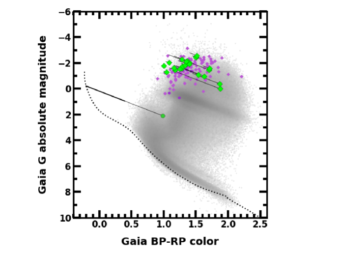
Figure 1: Color-magnitude diagram for stars in the Gaia DR2 archive with 5-$\sigma$ parallaxes and complete velocity measurements. The light gray points and shaded region show the distribution of the $N_{\textit{s}}\approx 1.5$-million sources with these properties (the shading is proportional to the logarithm of the density of stars in the plot). Main sequence stars are well defined on the lower left edge; giants lie above them. The magenta diamonds indicate stars that are marginally bound ($0.2\leq p_{\text{unb}}<0.5$); the lime-green diamonds are the unbound candidates ($p_{\text{unb}}\geq 0.5$). The darker shade of green or magenta circles indicate sources that have the duplicated_source flag raised. For the unbound candidates, we also correct for reddening as described in text; the tips of the thin black lines indicate the estimated intrinsic color and brightness. The faintest and bluest unbound star, located toward the Galactic Center, has intrinsic color and magnitude that suggests it is on the main sequence (indicated by the dotted curve, based on Marigo et al. 2017 for a 100-Myr isochrone with a metallicity of 0.01520). The thicker black line indicates a range of reddening and extinction corrections, with the Marshall et al. (2006) dust map giving the smaller correction and the Schlafly & Finkbeiner (2011) estimate giving the upper limit.

To estimate reddening corrections for the 25 unbound candidates, we use the IPAC/IRSA DUST service, based on the work of Schlegel et al. (1998) and Schlafly & Finkbeiner (2011). With a default Image Size of 5 degrees, we obtain the color excess, $E(B-V)$, and optical extinction, $A_{V}=3.1E(B-V)$, for each star. To convert to Gaia passbands, we follow the prescriptions in Cardelli et al. (eqs. (1) and (3) 1989) to get $A_{\lambda}/A_{V}$ where $A_{\lambda}$ is the extinction in a passband centered on wavelength $\lambda$. For the Gaia G band, $\lambda=637$ nm; the Gaia Blue Photometer (BP) and Red Photometer (RP) bands are centered on 532 nm and 797 nm, respectively (Jordi et al., 2010). The result is

$$E(\text{BP-RP})\approx 1.355E(B-V)\ \ \ \text{and}\ \ \ A_{G}\approx 0.848A_{V}.$$ (11)

Since Schlegel et al. (1998) and Schlafly & Finkbeiner (2011) provide total dust screening in the plane of the sky averaged over degree scales, $A_{G}$ and $E(\text{BP-RP})$ for nearby sources at low Galactic latitudes are approximate upper limits.

After correction for reddening, all but one of these fast stars has color and luminosity indicative of the low metallicity, low surface-gravity late-type giants identified by Hattori et al. (2018a) and Hawkins & Wyse (2018, see also ). Even with significant adjustments to our reddening correction, our interpretation of these sources as late-type giants remains the same.

Of the fast stars, Gaia DR2 5932173855446728064 is the most reddened. It lies within a few degrees of the Galactic plane and is the closest of the fast stars to the Sun (${d}_{\text{h}}=2.2$ kpc; see also Marchetti et al., 2018b). The 2-D V band extinction from Schlafly & Finkbeiner (2011) at this source’s location is $E(B-V)=0.88$, which is likely an upper bound. A refined estimate, based on the 3-D, low-latitude map by Marshall et al. (2006, which we access through the mwdust package) gives $E(B-V)=0.43$. Since small-scale variations in the dust (e.g., Minniti et al., 2018) may impact the actual reddening of this source, we indicate both estimates in Figure 1 (the Schlafly & Finkbeiner (2011) and Marshall et al. (2006) reddening agree to within 0.05 mag for other high-speed, low-latitude sources reported here). Despite these uncertainties, the corrected $M_{G}$ and BP-RP color are consistent with an early-type star either on the main sequence or one that is just evolving off it. Follow-up spectroscopy would distinguish these possibilities.

In Figure 1, the fastest stars are among the most luminous objects with 5-$\sigma$ parallaxes and complete velocity measurements. Compared to the bulk of the $\sim 1.5$M stars in Figure 1, our high-speed candidates typically have a large heliocentric distance. All but one lie outside of ${d}_{\text{h}}=5$ kpc. Because it is more challenging to acquire high quality astrometry for more distant objects, it is important to consider whether these high speed stars have measurement uncertainties similar to those of more slowly moving stars. Figure 2 shows that our fastest-moving stars, with one exception, have uncertainties in Galactocentric speed that scale with the speed. The key message from this figure, along with the color-magnitude data, is that our fastest moving objects are the most distant, most luminous ones with the biggest uncertainty in speed.

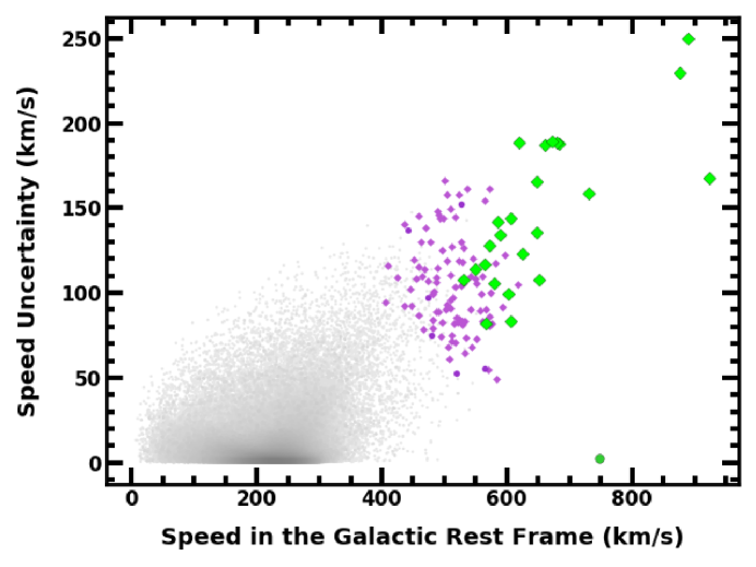
Figure 2: The uncertainty in Galactic rest-frame speed as a function of distance from the Galactic Center. The meaning of the symbols is as in Figure 1: Lime symbols are unbound candidates, magenta symbols are marginally bound, and the gray shading indicates the number density of the bulk of the $\sim$1.5M sources in our 6-D sample.

3.2 Orbital characteristics

To illustrate how the orbits of the fastest stars compare with the bulk of the $\sim$1.5M stars in the sample, we present a few different views of the data in Figure 3. We look at the speed of stars and their direction of travel in ways that highlight the difference between disk stars, the halo population, and unbound HVS or HRS orbits. In the Figure, we distinguish between the 25 unbound candidates (lime-colored symbols), the 101 nominally unbound objects (magenta circles), and the roughly $1.5$ million remaining stars.

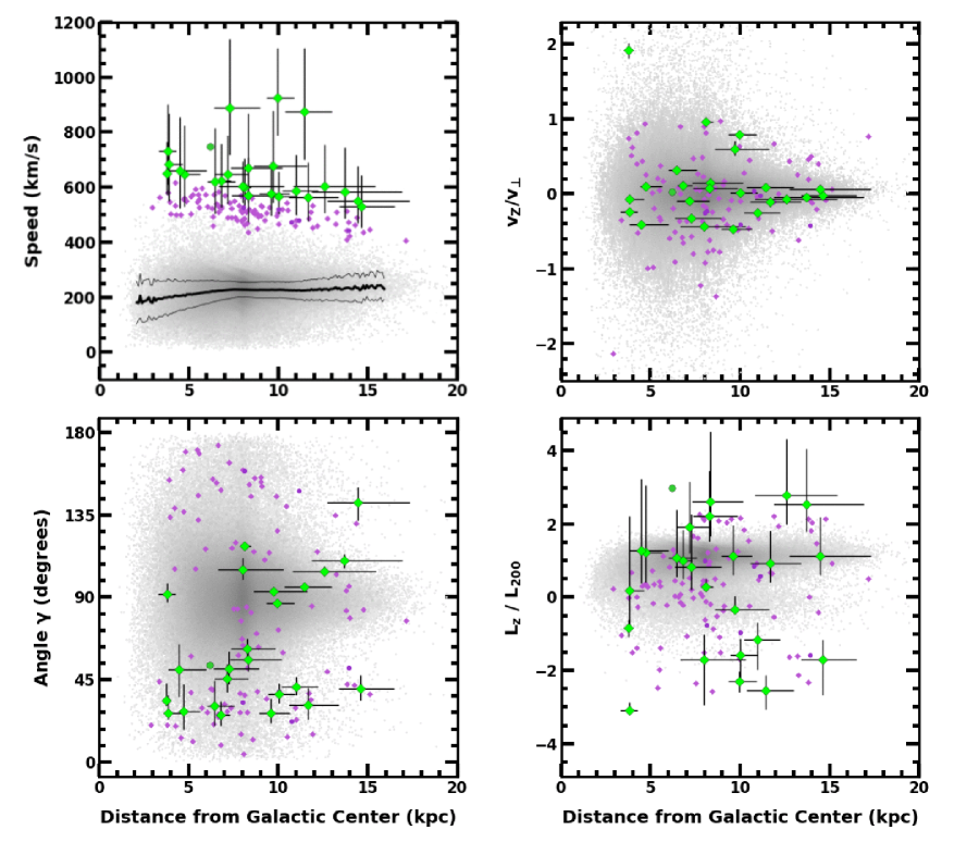
Figure 3: Orbit characteristics as a function of distance from the Galactic center of sample stars. As in Figure 1, lime-colored points represent unbound candidates ($p_{\text{unb}}\geq 0.5$); errorbars mark the 16-th to 84-th percentiles in the position and velocity distributions. The magenta points are nominally bound stars with at least 20% probability of being unbound ($0.2\leq p_{\text{unb}}<0.5$). The circle points show sources with the duplicated_source flag set, whereas diamonds indicate stars for which this flag is not raised. The light gray points are the remaining stars in our 6-D sample. The upper left panel shows Galactocentric speed, and the lower left shows the direction of travel relative to an outbound radial orbit. The upper right plot is the vertical speed relative to the plane-of-the-disk speed, and the lower right plot shows the $Z$-component of the angular momentum relative to the value characteristic of circular orbits in the disk ($L_{2}00$). Together, these plots build a picture of the high-speed stars as mostly outliers of the halo and disk populations. As a group, these stars also tend to be outgoing ($\gamma<90^{\circ}$ in the lower left panel). Their vertical motion is typically less than in the plane of the disk (upper right panel), and they tend to corotate with the Galactic disk (lower right panel). Despite significant uncertainties, the fastest objects are distinct from the bulk of sample, which has a mean speed near 200 km/s(thick line in the upper left plot) and 1-$\sigma$ range of $\lesssim 100$ kms (thinner lines).

The Galactic rest-frame speed of stars as a function of distance from the Galactic Center (Figure 3, upper left panel) gives an overall perspective of bound versus unbound candidates. The bulk of stars in the sample have considerably slower speeds, around 200 km/s. The dispersion is also low, $\sim 50$ km/s in the Solar neighborhood, suggesting that most of these stars are part of the disk. The dispersion creeps upward at larger distances and toward the Galactic Center at least in part because the uncertainty in speed (${\sigma}_{v,\text{g}}$) tends to increase with distance from the Sun.

Figure 3 also provides information about the orientation of stellar orbits. The lower left panel shows $\gamma$, the angle of travel relative to a purely radial trajectory, a measure tuned to select high-speed objects that originate from the Galactic Center ($\gamma=0^{\circ}$). The plot of ${v_{\text{Z}}}/v_{\bot}$ (upper right panel) measures the degree to which orbits are confined to the disk plane; $L_{\text{Z}}/L_{200}$, the $Z$-component of angular momentum relative to typical disk star values (lower right panel), provides information about the sense of orbital rotation compared with the disk. Together these panels illustrate that the majority of the $N_{\textit{s}}\approx 1.5$M stars shown in Figure 3 are associated with the disk: stars cluster around $\gamma=90^{\circ}$, ${v_{\text{Z}}}/v_{\bot}=0$ and $L_{\text{Z}}/L_{200}=1$. Another distinct population of stars is more evenly distributed in $\gamma$ and ${v_{\text{Z}}}/v_{\bot}$ and has values of $L_{\text{Z}}/L_{200}$ centered around zero. These are likely halo stars.

Within Figure 3, the marginally bound stars (magenta symbols) generally track our expectation of halo stars. There are roughly as many incoming as outgoing objects, with $\gamma$ values loosely clustered about $\sim 30^{\circ}$ and $\sim 150^{\circ}$. The mean and dispersion of ${v_{\text{Z}}}/v_{\bot}$ is characteristic of isotropic orbits. Furthermore, comparable numbers of these stars corotate with the Milky Way’s disk as counterrotate.

Among the 25 unbound candidates (lime-green symbols), the distribution suggests a trend toward orbits that are outgoing from the Galactic Center and co-rotating with the disk. Roughly two-thirds are on outgoing orbits (17 of 25 stars); a majority corotates with the disk (16 stars). Almost half of these sources have both of these characteristics (12 objects). Thus, while no compelling HVS candidates emerge, there is a hint that of some of the unbound candidates are HRSs.

3.3 Are the outliers really unbound?

The top 25 high-speed stars may include unbound HVS and HRS candidates (Kenyon et al., 2014, 2018). However, they may simply be slower-moving bound objects with large errors, drawn from the large pool of almost 1.5 million stars. When the unbound probability of a source has a modest value, different from unity (e.g., $p_{\text{unb}}\sim 0.5$), we cannot distinguish the unbound cases from the bound outliers. Even when $p_{\text{unb}}$ for a candidate is close to unity, we must consider whether it is a rare outlier of the bound population.

To develop an approach for distinguishing a truly unbound object from a bound outlier, we examine each unbound candidate and ask whether known bound stars could have been measured with an unbound probability as large as the candidate’s. Thus, we run through the long list of nominally bound stars ($p_{\text{unb}}<0.5)$, identifying those with uncertainties in Galactic distance and speed that are similar or better than the candidate’s. Then, by sampling the error distributions of these bound objects, we determine the probability, $p_{\textit{b,out}}$, that each bound star would be observed to be an unbound object like the candidate. If the candidate were just an outlier, then we expect $p_{\textit{b,out}}$ to be significant for at least some bound stars; if no bound star has any likelihood of being observed as an outlier with similar properties ($p_{\textit{b,out}}=0$), then the candidate stands out as a true unbound star.

In our algorithm for quantifying whether a star is unbound or an outlier, we work with the list of bound stars that have the same or smaller relative uncertainties, ${\sigma}_{r,\text{g}}/{r}_{\text{g}}$ and ${\sigma}_{v,\text{g}}/{v}_{\text{g}}$, compared to the candidate. For the $i$-th bound star on the list, Quasi-Monte Carlo trials give samples of the state vector in Galactic coordinates, based on the measured astrometry and uncertainties. A separate Quasi-Monte Carlo estimate gives the unbound probability $p_{\text{unb}}$ for each state vector. The fraction of trials that give $p_{\text{unb}}$ equal to or greater than that of the unbound candidate is our estimate of $p_{\textit{b,out}}$ the chance that a bound star would be identified as unbound, like the candidate.

The likelihood that an unbound star is not just an outlier comes from tallying up the possibilities that individual bound stars might be perceived as unbound,

$$p_{\textit{b}}=1-\prod_{i}(1-p_{\textit{b,out}}^{(i)}),$$ (12)

where the index $i$ runs over the list of bound stars. Similarly, the typical number of bound stars that are expected to be outliers like the candidate is

$$N_{\textit{b}}\sim\sum_{i}p_{\textit{b,out}}^{(i)}.$$ (13)

Thus, if none of the bound stars has as much of a chance of being an outlier as the unbound candidate ($p_{\textit{b,out}}=0$ for all $N_{\textit{s}}\approx$1.5M stars), $N_{\textit{b}}=0$. The candidate then has zero probability of being a bound outlier; it is probably unbound. If $p_{\textit{b}}$ is much less than unity, then we cannot distinguish the candidate from the unbound population.

Applied to our high-speed sample, this analysis yields two sources, Gaia DR2 5932173855446728064 and 1383279090527227264, as the most likely unbound stars. For the first source, the likelihood of drawing bound outliers with its orbital characteristics and measurement errors is formally zero ($p_{\textit{b}}=0$). None of the roughly 6 billion Quasi-Monte Carlo samples yields as extreme an outlier ($N_{\textit{b}}=0$), primarily because of the candidate’s high speed with small uncertainty ($747\pm 3$ km/s). The second source, Gaia DR2 1383279090527227264, also has a formal 100% probability of being an unbound star and not an outlier of the bound population.

Of the remaining sources, Gaia DR2 1478837543019912064 has the greatest chance of being an unbound star. There is an 86% chance that it is not just a bound outlier, although we expect that one star from a bound population would be an outlier as extreme as this star ($N_{\textit{b}}=0.99$). Gaia DR2 6456587609813249536 is a runner-up, with a 49% chance of being unbound given the pool of other sources ($N_{\textit{b}}=0.98$). The remaining 21 objects have more than a 99% chance of being bound outliers. These preliminary results do not indicate that these candidates are really bound; they just cannot be distinguished from bound outliers (see also Bromley et al., 2006; Brown et al., 2007a; Kenyon et al., 2018).

We summarize aspects of the two main candidates, including their orbits in the Galaxy. We use a simple, fixed-timestep, fourth-order orbit integrator to estimate how an object moves within our choice of Galactic potential (the integrator is similar to the one described in Kenyon et al., 2018).

• Gaia DR2 5932173855446728064: This star has a high radial velocity with low uncertainty ($v_{\text{r}}=747\pm 3$ km/s) (cf. Marchetti et al., 2018b). At a Galactocentric distance of ${r}_{\text{g}}=6.2\pm 0.1$ kpc, its radial motion alone indicates that it is gravitationally unbound. With position $(X,Y,Z)=(-6.1,-1.1,-0.1)$ kpc and speed $(U,V,W)=(-549,506,18)$ km/s, it is moving outward and with the rotation of the Galaxy, skimming the underside of the disk. A traceback of its orbit gives a closest approach to the Galactic Center of 4.8 kpc, at a distance of about 0.2 kpc below the plane. Because the star’s orbit is deflected upward by the gravity of the Galaxy, the star formally crossed the disk on the far side from the Sun (${r}_{\text{g}}\sim 20~{}kpc$), within the past 50 Myr. The reddening and extinction also suggest that this source may be an A-type main sequence star. Thus it may well be a hyper-runaway star of Galactic origin. However, this source is in a crowded field and has been flagged as a duplicated_source in the Gaia DR2 archive. Follow-up observations would resolve these ambiguities.

• Gaia DR2 1383279090527227264: At a distance of $10.0\pm 0.9$ kpc and with a speed of $924\pm 168$ km/s relative to the Galactic Center, this object is likely to be unbound (see also Marchetti et al., 2018b). It is situated well above the disk ($X,Y,Z=-5.7,5.1,6.4$ kpc) and its orbit arches upward and against the rotation of the disk ($U,V,W=-91,-719,573$ km/s). An orbit calculation back to the disk suggests an intersection at a distance just inside of 14 kpc from the GC about 15 Myr ago. An integration farther back in time gives an orbit that crosses within about 15 kpc of the Large Megellanic Cloud roughly 70 Myr ago. (One other star, Gaia DR2 6492391900301222656, has a similar closest approach to the LMC.) Thus, this star has promise as a hyper-runaway star candidate, or even an escapee from the LMC. Despite these intriguing possibilities, the kinematics, compared with the bulk of the 6-D samplei, and the source’s position in the color-magnitude diagram remind that it is probably a statistical high-speed outlier of the halo’s late-type giant population.

3.4 The impact of distance estimation

The results presented in this section come from a Quasi-Monte Carlo analysis in which heliocentric distances and parallaxes are related simply by ${d}_{\text{h}}=1/\varpi$. A Bayesian approach (§2) applied to the 5-$\sigma$ sample alters Galactocentric position and velocities only modestly, but the impact on the unbound probabilities $p_{\text{unb}}$ can be more substantial. For example, a prior for constant source density within roughly 20 kpc of the Sun ($L=40$ kpc in equation (2), motivated by HVS ejection models (Bromley et al., 2006)), yields 99 stars with $p_{\text{unb}}\geq 0.5$, including all of the sources listed in Tables 1 and 2. This increase arises because the prior causes distance estimates to increase, in accordance with the assumption that there are more sources at larger distances, at least for the parallax range of the 5-$\sigma$ stars. This change raises the tangential speed $v_{\text{t,g}}$ and the unbound probability $p_{\text{unb}}$.

A Bayesian prior that roughly follows the distance distribution of the bulk of the Gaia stars (equation (2) with $L=1.5$ kpc; cf. Bailer-Jones et al. 2018) tends to shift raw parallaxes toward the peak of the distance distribution of the bulk (${d}_{\text{h}}=2L$). More distant stars are estimated to be closer to the Sun, decreasing the tangential speed and the unbound probability The opposite happens for close-in stars. Both effects are present in our data. Analysis with this prior yields 16 stars with $p_{\text{unb}}\geq 0.5$; Of the 25 stars in Table 2, 13 appear in the new catalog. The drop-outs are have $p_{\text{unb}}<0.75$, and are at median distances ${d}_{\text{h}}>8$ kpc. Three new candidates emerge (Gaia DR2 3905884598043829504, Gaia DR2 3705761936916676864 and Gaia DR2 6516009306987094016), all with comparatively small distances, below about 5 kpc, and unbound probabilities near our 50% threshold.

Adopting a larger value of scale length $L$ in the exponential prior, as in Marchetti et al. (2018b), gives results that are more similar to the ones presented here. The heliocentric distance estimates between the two cases change typically by a few percent or less. The exponential model draws in 11 new objects with $p_{\text{unb}}$ near the 50% threshold, and of the 25 high-speed stars identified here, only one star, the object with the lowest $p_{\text{unb}}$, falls below the threshold as a result of the prior.

All of the distance estimation methods explored here yield the same set of stars with high probability of being unbound to the Galaxy, with $p_{\text{unb}}>0.75$ in Table 2. Thus, the identification of the most promising candidates is insensitive to the details of distance estimation, which is our motivation for selecting the 5-$\sigma$ sample.

4 INFERRING 3-D VELOCITY FROM PROPER MOTION OR RADIAL VELOCITY

In addition to finding unbound candidates, our 6-D sample allows evaluation of other measures of velocity as indicators of stellar orbits. Figure 4 shows the radial velocity in the Galactic frame, $v_{\text{r,g}}$ ($v_{\text{r}}$ corrected for Solar motion). One star, the top unbound candidate Gaia DR2 5932173855446728064, stands out with a high radial speed, $v_{\text{r,g}}>{v}_{\text{esc}}$. With ($\ell,b)=(329.94^{\circ},-2.70^{\circ})$, it lies inside the Solar circle, roughly in the direction of the Galactic Center relative to the Sun, and is approaching the Sun with a closing speed of over 600 km/s (Marchetti et al., 2018b).

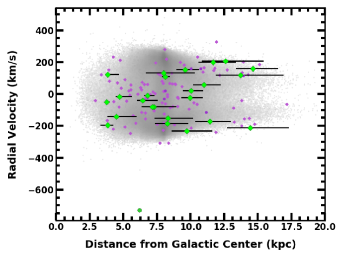
Figure 4: The radial velocity of stars, corrected for Solar motion. The symbols are the same as in the preceding Figures; lime-green points are unbound ($p_{\text{unb}}\geq 0.5$), magenta points are marginally bound ($0.2\geq p_{\text{unb}}<0.5$), and the remaining 1.5M stars are represented in gray. Except for two outliers, the unbound or marginally bound stars are mixed in with the slower-moving objects. Radial velocity is not a strong discriminant for high-speed stars in this sample.

Figure 4 reveals a second outlier, Gaia DR2 1364548016594914560, a marginally bound star (the uppermost magenta point in the Figure). This source lies beyond the Solar circle and is on an orbit that is nearly radially outward from the Galactic Center. Although it was tagged as a hypervelocity candidate by Marchetti et al. (2018b), it is not included in our top-25 list; our choice of Galactic potential suggests that this star is most likely bound to the Galaxy (see also Brown et al., 2007a).

Other than the two outliers, the stars shown in Figure 4 have radial speeds of less than $\sim$300 km/s. Thus, the $v_{\text{r,g}}$ values of the high-speed outliers give little indication of unusual motion. Radial velocities alone do not consistently distinguish high-speed stars from bound disk or halo stars at the modest Galactocentric distances discussed here.

Figure 5 shows the tangential speed of stars in our sample, $v_{\text{t,g}}$, derived from parallax and proper motion, and corrected for Solar motion. Nearly all of the high-speed stars that we identify as either unbound or marginally bound lie in the upper envelop of the speed distribution. Thus, in contrast to radial velocity, proper motion leads to a more robust indicator of speed relative to the Galactic Standard of Rest, at least for stars within $\sim$10 kpc of the Sun. The one exception to this rule is the radial-velocity outlier, Gaia DR2 5932173855446728064, which exhibits comparatively little tangential motion.

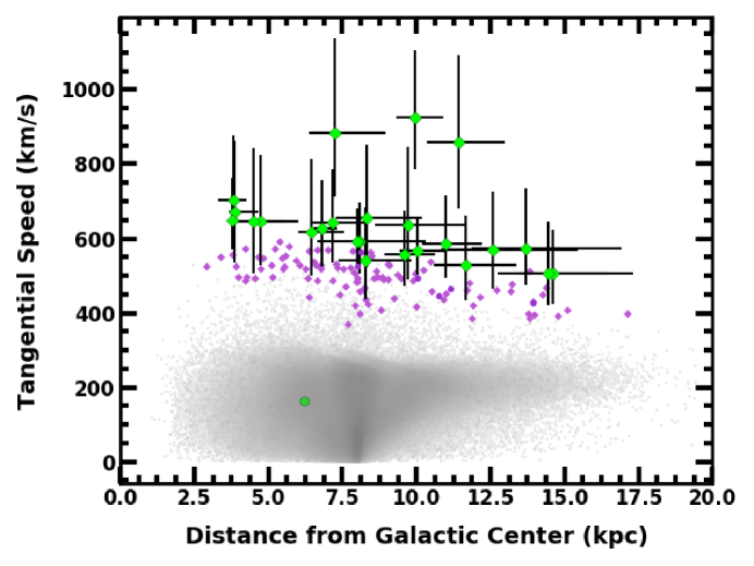
Figure 5: The tangential speed of stars, corrected for Solar motion. The symbols are the same as in the previous plot. Here, the tangential motion leads to a clustering of high-speed stars roughly sorted by probability of being unbound to the Galaxy. The one exception is the lime-colored point below $v_{\text{t,g}}=200$ km/s; its motion, relative to the Sun, is predominantly radial.

For stars at the modest heliocentric distances in our sample, tangential velocity is a good measure of the probability that a star is unbound. This result contrasts with more distant samples, where the radial velocity selects robust samples of unbound stars (e.g., Brown et al., 2006a, 2009, 2014). Figure 6 shows the Galactocentric speed of stars in our sample as a function of unbound probability $p_{\text{unb}}$.

We also show the unbound probability as determined from radial and tangential speeds separately. The distributions of these sets of points illustrate that tangential speed is a reasonable indicator of $p_{\text{unb}}$. Radial velocity measurements on their own mostly fail to predict $p_{\text{unb}}$. Thus, for nearby stars with distances of 10–15 kpc, selection according to proper motion and parallax is an efficient way to find high-speed stars. In our sample, identifying stars with tangential speeds exceeding 0.75 times local escape speed selects 92% of the stars that are unbound to the Galaxy with $p_{\text{unb}}$ = 20% or higher, with a false detection rate of 43%. In contrast, identifying nearby, high speed stars solely by radial velocity yields only one candidate (Gaia DR2 5932173855446728064).

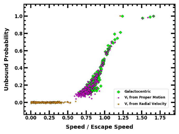
Figure 6: Probability that a star is unbound to the Galaxy, as a function of speed in the Galactic rest frame. The speed of each star is derived in three ways: from radial velocity $v_{\text{r,g}}$ alone (orange triangles), tangential speed $v_{\text{t,g}}$ alone (magenta circles), and the total Galactocentric speed ${v}_{\text{g}}$ (lime diamonds; each star has three points associated with it). Only the last set of points, derived from both radial and tangential motion, gives the true unbound probability, $p_{\text{unb}}$. The tangential data track the true probability reasonably well. The radial velocity data fail miserably, but not completely, in predicting $p_{\text{unb}}$. The one exception is the high-speed radial velocity outlier (the upper orange triangle, which corresponds to the green diamond to its immediate right). Only stars with $p_{\text{unb}}>0.01$ are considered in this analysis.

5 NEW CANDIDATES IN 5-D

From the 6-D analysis of §4 and the calculations of HVSs in Kenyon et al. (2018), measurements of tangential velocity provide a good indicator of nearby (10–15 kpc) high-speed stars, including those on orbits that emanate radially outward from the Galactic Center. We now consider stars in the full Gaia DR2 archive that satisfy the astrometric criteria listed in §2 yet do not have radial velocity measurements. Our analysis of these sources is as described in §2, except with no radial velocity component. Because we are most interested in fast stars, we consider a subset of these sources that have an observed tangential speed, corrected for Solar motion, of $v_{\text{t,g}}>400$ km/s (approximately 70% of the escape speed in the Solar neighborhood). This sample of 9939 fast-moving objects contains the most promising unbound candidates in 5-D.

The proper motion sample includes 343 stars with $\geq$ 50% likelihood of being unbound ($p_{\text{unb}}\geq 0.5)$. Of these, 19 are unbound with 95% confidence on the sole basis of tangential velocity and astrometric uncertainties. Table 3 summarizes the properties of these 19 fastest objects. Figure 7 provides brightness and color information of all stars in this sample, with indicators of reddening and extinction from the IPAC/IRSA DUST service. The most significantly reddened sources (Gaia DR2 2946665465655257472 and Gaia DR2 1820299950021811072) are both within 10^∘ of the Galactic plane; nonetheless the values of $E(B-V)$ provided by IRSA (0.497 and 0.287, respectively) are within 0.1 mag of the estimate from the 3-D Combine15 maps in the mwdust package (Bovy et al., 2016). Figure 8 shows the Galactocentric distance and speed information for all stars in this sample.

From this subset of the Gaia DR2 archive, we conclude that the high-speed stars in 5-D are more broadly representative of the general population of stars in the Milky Way. We have not evidently selected an exclusive set of HVS or HRS candidates. Instead, we speculate that these stars, like the majority of our high-speed candidates in 6-D, are outliers of a bound distribution. Radial velocity measurements of these top candidates are required to test this interpretation.

Table 3: High-speed stars: tangential speed selection.

Gaia DR2	G	BP-RP	($\ell$,$b$)	${d}_{\text{h}}$	${r}_{\text{g}}$	$v_{\text{t,g}}$	$p_{\text{unb}}$
designation	(mag)	(mag)	(deg)	(kpc)	(kpc)	(km/s)
1540013339194597376	15.96	1.01	(145.31, 68.25)	1.70$\pm$0.16	8.7$\pm$0.1	917.2$\pm$107.1	1.00
1240475894700468736	14.03	0.99	( 20.41, 67.83)	3.99$\pm$0.47	7.6$\pm$0.1	842.6$\pm$124.1	1.00
1570348658847157888	15.63	0.74	(122.23, 62.07)	5.07$\pm$0.79	10.5$\pm$0.6	885.7$\pm$179.0	1.00
1312242152517660800	13.81	0.30	( 50.78, 40.14)	8.39$\pm$1.52	8.3$\pm$0.9	837.0$\pm$172.1	0.99
4727516205455716224	13.57	0.63	(273.60,-51.39)	8.84$\pm$1.26	11.7$\pm$0.9	740.7$\pm$117.2	0.99
1586391907885793792	14.39	0.64	( 78.07, 57.23)	10.34$\pm$2.32	12.3$\pm$1.9	873.4$\pm$244.0	0.99
5778956291515661440	14.31	0.99	(313.01,-19.17)	8.45$\pm$1.39	6.9$\pm$0.8	852.1$\pm$168.5	0.99
4798132614628163968	15.92	0.62	(253.31,-35.03)	5.69$\pm$1.24	10.9$\pm$0.9	819.0$\pm$194.7	0.99
1820299950021811072	14.01	1.34	( 54.89, -6.08)	7.66$\pm$1.57	7.3$\pm$0.9	877.3$\pm$208.9	0.99
2946665465655257472	16.22	1.09	(227.47, -9.16)	3.17$\pm$0.66	10.4$\pm$0.6	786.7$\pm$173.6	0.98
1527780516422382592	15.14	0.77	(117.82, 74.69)	4.03$\pm$0.58	9.4$\pm$0.3	765.5$\pm$135.7	0.98
4535258625890434944	13.14	1.18	( 52.01, 14.00)	5.31$\pm$0.41	6.4$\pm$0.0	688.4$\pm$55.2	0.98
1702417150851952128	13.84	1.10	(107.08, 37.42)	11.39$\pm$2.19	15.4$\pm$1.9	728.7$\pm$160.8	0.97
4783869234396531968	15.44	0.84	(257.18,-38.70)	5.71$\pm$1.15	10.6$\pm$0.9	792.1$\pm$200.6	0.97
2154188852160448512	13.51	1.21	( 86.83, 24.49)	12.23$\pm$2.33	14.3$\pm$2.0	671.9$\pm$110.6	0.97
6524618551753693952	14.06	1.04	(328.60,-64.49)	7.86$\pm$1.50	8.9$\pm$1.0	795.0$\pm$190.1	0.96
1484524973071001984	15.83	0.64	( 68.04, 68.64)	4.50$\pm$0.77	8.6$\pm$0.3	779.1$\pm$170.1	0.96
6358539652542070912	13.95	1.21	(315.20,-37.99)	12.08$\pm$2.72	10.1$\pm$2.2	800.7$\pm$217.1	0.95
4805658359403594624	13.46	1.22	(249.38,-32.52)	15.25$\pm$3.61	19.2$\pm$3.3	710.0$\pm$194.2	0.95

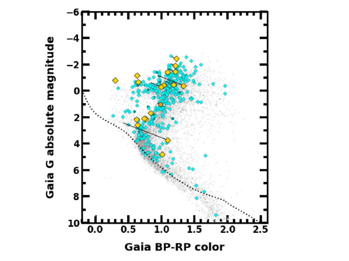
Figure 7: The color-magnitude diagram of stars in the Gaia DR2 with 5-$\sigma$ astrometry but no radial velocity measurement. The dotted line shows the position of the main sequence. All stars with $v_{\text{t,g}}>400$ km/s are shown in gray. The cyan diamonds indicate stars with $p_{\text{unb}}\geq 0.5$; the yellow-gold diamonds plot the subset with $p_{\text{unb}}\geq 0.95$. Darker-shaded circles show sources that have the duplicated_source flag set. Thin solid lines indicate reddening vectors. Unlike the 6-D data, the fastest stars include those near the main sequence as well as late-type giants.

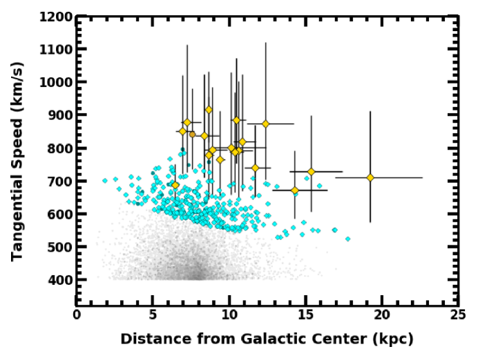
Figure 8: The Galactic-frame tangential speed of fast-moving stars in the Gaia DR2 with 5-$\sigma$ astrometry but no radial velocity measurement. As in Figure 7, yellow-gold symbols plot stars with probability $p_{\text{unb}}\geq 0.95$; cyan points correspond to stars with $0.5\leq p_{\text{unb}}\leq 0.95$; gray points indicate stars with $v_{\text{t,g}}>400$ kms and $p_{\text{unb}}\leq 0.5$. This sample and the theoretical analysis of Kenyon et al. (2018) suggest that the high-speed stars are excellent candidates for HVSs and HRSs.

The list in Table 3 with $p_{\text{unb}}\geq 0.95$ changes in a Bayesian analysis. As with the 6-D sample, a prior tuned for a uniform source density within the Milky Way yields larger distance estimates and is more permissive in the assessment of whether a star is unbound. It yields 90 sources, including the 19 stars in the Table. An analysis with an exponential prior and $L=1.5$ kpc (equation (2)) flags 17 stars with $p_{\text{unb}}\geq 0.95$, 15 of which are in Table 3. Two are new candidates (Gaia DR2 6182941362050295424 and Gaia DR2 6698855754225352192) within 6 kpc of the Sun. The four from the Table that are missed by the Bayesian analysis all have estimated median distances beyond 10 kpc. All three methods identify the same highest speed sources with $p_{\text{unb}}>0.98$.

6 COMPARISON WITH THEORY

Kenyon et al. (2018, Figures 21 and 22 therein) predict that HVSs and HRSs are efficiently selected at heliocentric distances well beyond $\sim 10$ kpc with radial velocities. At these distances, tangential motion is not significant. Closer to the Sun and to the Galactic Center, radial velocities may be significant, but will not typically differ much from the motion of bound halo stars. Tangential speeds, however, will be high for nearby HVSs and HRSs. Radial velocities select high-speed stars at large distances; proper motion selects the fastest-moving stars within $\sim 10$ kpc.

Our analysis, based on 6-D data but using only 5-D information for comparison, confirms the geometrical argument in Kenyon et al. (2018). All of the high-speed outliers, with one exception, have large tangential speeds and nondescript radial speeds. The exception, Gaia DR2 5932173855446728064, is an unusual star, seemingly coming nearly directly toward the Sun in the heliocentric frame. Figures 4 and 5 illustrate these effects.

We also have sought to identify HVS and HRS candidates in the 6-D data. Focusing on the top 101 high-speed stars, only Gaia DR2 5932173855446728064 has a high probability of being unbound, a low likelihood that it is an outlying bound star, and spectral type suggesting a young main sequence star. Other stars are more suggestive of sample outliers of the halo’s late-type giant population. None of the stars has a radial direction of travel ($\gamma$ near 0^∘). A Galactic Center origin for this population is not favored.

The small number of HVSs is expected. The sample region is small (a radius of $\sim 10$ kpc), compared to the region of space explored in HVS searches of the Milky Way halo (out to $\sim 100$ kpc; Brown et al., 2005, 2006a, 2007a, 2014). Theory predicts few if any A- or B-type stars on hypervelocity trajectories in this small region (e.g., Hills, 1988; Yu & Tremaine, 2003; Bromley et al., 2006; Kenyon et al., 2014; Hamers & Perets, 2017); observations support this assessment (e.g., Brown et al., 2006a; Kollmeier & Gould, 2007; Kollmeier et al., 2009, 2010; Brown et al., 2014). On the basis of the relatively short lifetimes of giants compared to these main sequence stars, the likelihood of observing an evolved star in this region is even lower.

HRSs may arise from binary supernova ejection (e.g. Poveda et al., 1967; Leonard, 1991; Wang & Han, 2009; Tauris, 2015) or dynamical ejections, boosted by Galactic rotation (e.g., Blaauw, 1961; De Donder et al., 1997; Portegies Zwart, 2000). Other mechanisms, such as tidal shredding of dwarf galaxies by the Milky Way (Abadi et al., 2009; Piffl et al., 2014) are other possibilities. The expected number of HRSs among early-type stars is nonetheless somewhat lower than for HVSs (e.g., Perets, 2009; Brown et al., 2015). Still, the detection of a single high-speed star with a Galactic disk origin, if confirmed, is likely not a strong challenge to theoretical predictions.

We caution that these inferences about the number counts are only preliminary, order-of-magnitude estimates. The Gaia DR2 archive is not uniform on the sky with respect to the selection criteria we use in deriving the sample with 5-$\sigma$ astrometry.

Our reliance on the errors in parallax and proper motion to make robust estimates for $p_{\text{unb}}$ assumes that the noise in not sensitive to motions not included in model fits to Gaia astrometric data. For example, the Gaia DR2 astrometric solution does not model binary motion (Lindegren et al., 2018). Stars in binaries with orbital periods of 1–3 yr have semimajor axes of several tenths of a mas at distances of roughly 10 kpc; this unmodeled motion could inflate the parallax, proper motion, and associated errors. Future Gaia releases will include data that cover a typical orbital period for these binaries and a model that solves for binary motion. This analysis should clarify the relationship between the error in the speed and the speed for the highest velocity stars.

7 CONCLUSION

We analyze a sample of approximately 1.5 M stars with measured radial velocity and 5-$\sigma$ parallaxes from Gaia DR2 using a fast and accurate Quasi-Monte Carlo algorithm. The code incorporates Bayesian distance estimation and accommodates correlated erros in Gaia DR2 basic source parameters. All of the stars lie within about 15 kpc of both the Sun and the Galactic Center. Using their total space motion in the Galactic rest-frame, we identify the most promising HVS and HRS candidates. Considering only the stars’ radial velocity or proper motion, we conclude that the Galactic rest-frame radial velocity provides a poor measure of total space motion for the fastest stars. However, the tangential velocity alone is sufficient to identify unbound star candidates within $\sim$15 kpc of the Sun.

We determine Galactocentric locations and speeds, along with uncertainties, to find the probability that each source in our sample is unbound to the Galaxy. This probability, $p_{\text{unb}}$, depends on the choice of Galactic potential (we use the model in Kenyon et al., 2018), the quality of the astrometric data, and the method of distance estimation from parallax. To reduce the impact of prior assumptions about source location on heliocentric distance estimation, we work with sources that have relative parallax errors of 20% or less. An analysis with a heliocentric distance prior based on the bulk of Gaia stars gives similar results to an analysis where all parallaxes in the error distribution out to 5-$\sigma$ give physically plausible distances. Other assumptions, including a constant distribution of sources in space, admit more possibilities. We are encouraged that all methods, even the more restrictive ones, yield the same set of stars that have a high probability of being unbound.

However, even when a star has $p_{\text{unb}}$ near unity, it is only one of over 1.5 M stars with 5-$\sigma$ astrometric and radial velocity data. For stars with large measurement errors, we expect to find statistical outliers drawn from the enormous bound population. Thus, we introduce an analysis to address quantitatively whether a star is truly unbound or whether its observed kinematics are consistent with a bound statistical outlier of a large sample. This analysis suggests that most high speed stars in the 6-D sample are bound outliers.

Other features of the highest-speed stars support the case against unbound orbits. They have large errors in Galactocentric speed and are probably late-type giants with lifetimes rather short compared to the time scale for unbound stars to escape the Galaxy ($\sim 100$ Myr). While there may be some physical explanation for the coincidence in timing, the idea that these stars are outliers due to the large velocity errors is compelling. We suspect that many of the objects identified by Marchetti et al. (2018b) and Hattori et al. (2018a), also predominantly late-type giants, are bound outliers as well.

There is at least one promising object in our high-speed sample, (Gaia DR2 5932173855446728064), first identified by Marchetti et al. (2018b), with the orbital elements of a star that is unbound to the Galaxy at a high level of confidence (§3.3). With colors (albeit reddened) that suggest an A-type main sequence star, and an orbit that runs close to the Galactic plane, this object is a hyper-runaway star candidate (Marchetti et al., 2018b). However, a Gaia DR2 error flag is set, so we emphasize the need for observational confirmation of the source’s orbital parameters.

Twenty four other high-speed sources have trajectories and colors consistent with late-type giants that make them improbable HVS or HRS candidates. Our analysis of the likelihood that these objects are unbound suggests these stars are statistical outliers of the Milky Way’s bound population. Nonetheless, these stars are excellent candidates for programs to obtain high quality ground-based spectra. One of these stars, Gaia DR2 1383279090527227264, stands out, with the lowest probability that it is just an outlier. This object and another star in this group (Gaia DR2 6492391900301222656) have orbits that passed near the LMC. Subsequent Gaia data releases with improved astrometry will allow refined orbit calculations and inferences about the origin of these high-speed stars.

Whether bound outliers or unbound stars, some of our highest-speed stars probably have a Galactic disk origin. A significant majority show angular momentum aligned with the Galaxy’s disk (Fig. 3, lower right panel). Most of this majority are also on trajectories that are outbound from the Galactic Center. An analysis of the type introduced here, to determine whether a source is actually an unbound star or an outlier, may be adapted to constrain the mass of the Milky Way inside 10-20 kpc as in Gnedin et al. (2005).

Motivated by our confirmation that proper motion alone can efficiently select nearby high-speed stars (§4; see also Kenyon et al. 2018), we identify new candidates selected from 5-D Gaia data. Even without radial velocities, 19 stars have unbound probabilities of 95% or more, with inferred speeds between about 600 kms and 900 km/s. Their colors and magnitudes suggest that this sample includes both main sequence stars as well as evolved giants. Better astrometry and radial velocity measurements will help us learn if these intriguing objects are among the fastest moving stars in the Galaxy.

References

- Abadi et al. (2009) Abadi, M. G., Navarro, J. F., & Steinmetz, M. 2009, ApJ, 691, L63
- Astraatmadja & Bailer-Jones (2016) Astraatmadja, T. L., & Bailer-Jones, C. A. L. 2016, ApJ, 832, 137
- Bailer-Jones (2015) Bailer-Jones, C. A. L. 2015, PASP, 127, 994
- Bailer-Jones et al. (2018) Bailer-Jones, C. A. L., Rybizki, J., Fouesneau, M., Mantelet, G., & Andrae, R. 2018, AJ, 156, 58
- Blaauw (1961) Blaauw, A. 1961, Bull. Astron. Inst. Netherlands, 15, 265
- Boubert et al. (2018) Boubert, D., Guillochon, J., Hawkins, K., Ginsburg, I., & Evans, N. W. 2018, ArXiv e-prints, arXiv:1804.10179
- Bovy (2015) Bovy, J. 2015, ApJS, 216, 29
- Bovy et al. (2016) Bovy, J., Rix, H.-W., Schlafly, E. F., et al. 2016, ApJ, 823, 30
- Bromley et al. (2009) Bromley, B. C., Kenyon, S. J., Brown, W. R., & Geller, M. J. 2009, ApJ, 706, 925
- Bromley et al. (2006) Bromley, B. C., Kenyon, S. J., Geller, M. J., et al. 2006, ApJ, 653, 1194
- Brown (2015) Brown, W. R. 2015, ARA&A, 53, 15
- Brown et al. (2015) Brown, W. R., Anderson, J., Gnedin, O. Y., et al. 2015, ApJ, 804, 49
- Brown et al. (2013) Brown, W. R., Cohen, J. G., Geller, M. J., & Kenyon, S. J. 2013, ApJ, 775, 32
- Brown et al. (2009) Brown, W. R., Geller, M. J., & Kenyon, S. J. 2009, ApJ, 690, 1639
- Brown et al. (2012) —. 2012, ApJ, 751, 55
- Brown et al. (2014) —. 2014, ApJ, 787, 89
- Brown et al. (2005) Brown, W. R., Geller, M. J., Kenyon, S. J., & Kurtz, M. J. 2005, ApJ, 622, L33
- Brown et al. (2006a) —. 2006a, ApJ, 640, L35
- Brown et al. (2006b) —. 2006b, ApJ, 647, 303
- Brown et al. (2007a) Brown, W. R., Geller, M. J., Kenyon, S. J., Kurtz, M. J., & Bromley, B. C. 2007a, ApJ, 660, 311
- Brown et al. (2007b) —. 2007b, ApJ, 671, 1708
- Brown et al. (2018) Brown, W. R., Lattanzi, M. G., Kenyon, S. J., & Geller, M. J. 2018, ArXiv e-prints, arXiv:1805.04184
- Callingham et al. (2018) Callingham, T., Cautun, M., Deason, A. J., et al. 2018, ArXiv e-prints, arXiv:1808.10456
- Caputo & degl’Innocenti (1995) Caputo, F., & degl’Innocenti, S. 1995, A&A, 298, 833
- Capuzzo-Dolcetta & Fragione (2015) Capuzzo-Dolcetta, R., & Fragione, G. 2015, MNRAS, 454, 2677
- Cardelli et al. (1989) Cardelli, J. A., Clayton, G. C., & Mathis, J. S. 1989, ApJ, 345, 245
- De Donder et al. (1997) De Donder, E., Vanbeveren, D., & van Bever, J. 1997, A&A, 318, 812
- Du et al. (2018) Du, C., Li, H., Liu, S., Donlon, T., & Newberg, H. J. 2018, ArXiv e-prints, arXiv:1807.00427
- Edelmann et al. (2005) Edelmann, H., Napiwotzki, R., Heber, U., Christlieb, N., & Reimers, D. 2005, ApJ, 634, L181
- Foreman-Mackey et al. (2013) Foreman-Mackey, D., Hogg, D. W., Lang, D., & Goodman, J. 2013, PASP, 125, 306
- Fragione & Capuzzo-Dolcetta (2016) Fragione, G., & Capuzzo-Dolcetta, R. 2016, MNRAS, 458, 2596
- Fritz et al. (2018) Fritz, T. K., Battaglia, G., Pawlowski, M. S., et al. 2018, ArXiv e-prints, arXiv:1805.00908
- Gaia Collaboration et al. (2018a) Gaia Collaboration, Brown, A. G. A., Vallenari, A., et al. 2018a, ArXiv e-prints, arXiv:1804.09365
- Gaia Collaboration et al. (2018b) —. 2018b, ArXiv e-prints, arXiv:1804.09365
- Gaia Collaboration et al. (2016) Gaia Collaboration, Prusti, T., de Bruijne, J. H. J., et al. 2016, A&A, 595, A1
- Gaia Collaboration et al. (2018c) Gaia Collaboration, Helmi, A., van Leeuwen, F., et al. 2018c, ArXiv e-prints, arXiv:1804.09381
- Gaia Collaboration et al. (2018d) Gaia Collaboration, Babusiaux, C., van Leeuwen, F., et al. 2018d, ArXiv e-prints, arXiv:1804.09378
- Gnedin et al. (2005) Gnedin, O. Y., Gould, A., Miralda-Escudé, J., & Zentner, A. R. 2005, ApJ, 634, 344
- Hamers & Perets (2017) Hamers, A. S., & Perets, H. B. 2017, ApJ, 846, 123
- Hattori et al. (2018a) Hattori, K., Valluri, M., Bell, E. F., & Roederer, I. U. 2018a, ArXiv e-prints, arXiv:1805.03194
- Hattori et al. (2018b) Hattori, K., Valluri, M., & Castro, N. 2018b, ArXiv e-prints, arXiv:1804.08590
- Hawkins & Wyse (2018) Hawkins, K., & Wyse, R. F. G. 2018, ArXiv e-prints, arXiv:1806.07907
- Hills (1988) Hills, J. G. 1988, Nature, 331, 687
- Hirsch et al. (2005) Hirsch, H. A., Heber, U., O’Toole, S. J., & Bresolin, F. 2005, A&A, 444, L61
- Ibata et al. (1998) Ibata, R. A., Lewis, G. F., & Beaulieu, J.-P. 1998, ApJ, 509, L29
- Johnson & Soderblom (1987) Johnson, D. R. H., & Soderblom, D. R. 1987, AJ, 93, 864
- Jordi et al. (2010) Jordi, C., Gebran, M., Carrasco, J. M., et al. 2010, A&A, 523, A48
- Kenyon et al. (2014) Kenyon, S. J., Bromley, B. C., Brown, W. R., & Geller, M. J. 2014, ApJ, 793, 122
- Kenyon et al. (2018) —. 2018, ArXiv e-prints, arXiv:1806.10167
- Kenyon et al. (2008) Kenyon, S. J., Bromley, B. C., Geller, M. J., & Brown, W. R. 2008, ApJ, 680, 312
- Kollmeier & Gould (2007) Kollmeier, J. A., & Gould, A. 2007, ApJ, 664, 343
- Kollmeier et al. (2009) Kollmeier, J. A., Gould, A., Knapp, G., & Beers, T. C. 2009, ApJ, 697, 1543
- Kollmeier et al. (2010) Kollmeier, J. A., Gould, A., Rockosi, C., et al. 2010, ApJ, 723, 812
- Leonard (1991) Leonard, P. J. T. 1991, AJ, 101, 562
- Lindegren et al. (2018) Lindegren, L., Hernandez, J., Bombrun, A., et al. 2018, ArXiv e-prints, arXiv:1804.09366
- Luri et al. (2018) Luri, X., Brown, A. G. A., Sarro, L. M., et al. 2018, A&A, 616, A9
- Marchetti et al. (2018a) Marchetti, T., Contigiani, O., Rossi, E. M., et al. 2018a, MNRAS, 476, 4697
- Marchetti et al. (2018b) Marchetti, T., Rossi, E. M., & Brown, A. G. A. 2018b, ArXiv e-prints, arXiv:1804.10607
- Marchetti et al. (2017) Marchetti, T., Rossi, E. M., Kordopatis, G., et al. 2017, MNRAS, 470, 1388
- Marigo et al. (2017) Marigo, P., Girardi, L., Bressan, A., et al. 2017, ApJ, 835, 77
- Marshall et al. (2006) Marshall, D. J., Robin, A. C., Reylé, C., Schultheis, M., & Picaud, S. 2006, A&A, 453, 635
- Minniti et al. (2018) Minniti, D., Saito, R. K., Gonzalez, O. A., et al. 2018, A&A, 616, A26
- Monari et al. (2018) Monari, G., Famaey, B., Carrillo, I., et al. 2018, ArXiv e-prints, arXiv:1807.04565
- Patel et al. (2018) Patel, E., Besla, G., Mandel, K., & Sohn, S. T. 2018, ApJ, 857, 78
- Perets (2009) Perets, H. B. 2009, ApJ, 690, 795
- Perets & Subr (2012) Perets, H. B., & Subr, L. 2012, ApJ, 751, 133
- Piffl et al. (2014) Piffl, T., Scannapieco, C., Binney, J., et al. 2014, A&A, 562, A91
- Portegies Zwart (2000) Portegies Zwart, S. F. 2000, ApJ, 544, 437
- Posti & Helmi (2018) Posti, L., & Helmi, A. 2018, ArXiv e-prints, arXiv:1805.01408
- Poveda et al. (1967) Poveda, A., Ruiz, J., & Allen, C. 1967, Boletin de los Observatorios Tonantzintla y Tacubaya, 4, 86
- Press et al. (1992) Press, W. H., Teukolsky, S. A., Vetterling, W. T., & Flannery, B. P. 1992, Numerical recipes in C. The art of scientific computing
- Raddi et al. (2018) Raddi, R., Hollands, M. A., Gänsicke, B. T., et al. 2018, MNRAS, arXiv:1804.09677
- Reid et al. (2014) Reid, M. J., Menten, K. M., Brunthaler, A., et al. 2014, ApJ, 783, 130
- Rossi et al. (2014) Rossi, E. M., Kobayashi, S., & Sari, R. 2014, ApJ, 795, 125
- Rossi et al. (2017) Rossi, E. M., Marchetti, T., Cacciato, M., Kuiack, M., & Sari, R. 2017, MNRAS, 467, 1844
- Schlafly & Finkbeiner (2011) Schlafly, E. F., & Finkbeiner, D. P. 2011, ApJ, 737, 103
- Schlegel et al. (1998) Schlegel, D. J., Finkbeiner, D. P., & Davis, M. 1998, ApJ, 500, 525
- Schönrich et al. (2010) Schönrich, R., Binney, J., & Dehnen, W. 2010, MNRAS, 403, 1829
- Sesana et al. (2006) Sesana, A., Haardt, F., & Madau, P. 2006, ApJ, 651, 392
- Sesana et al. (2009) Sesana, A., Madau, P., & Haardt, F. 2009, MNRAS, 392, L31
- Shen et al. (2018) Shen, K. J., Boubert, D., Gänsicke, B. T., et al. 2018, ArXiv e-prints, arXiv:1804.11163
- Sobol (1976) Sobol, I. 1976, USSR Computational Mathematics and Mathematical Physics, 16, 236
- Subr & Haas (2016) Subr, L., & Haas, J. 2016, ApJ, 828, 1
- Tauris (2015) Tauris, T. M. 2015, MNRAS, 448, L6
- Wang & Han (2009) Wang, B., & Han, Z. 2009, A&A, 508, L27
- Watkins et al. (2018) Watkins, L. L., van der Marel, R. P., Sohn, S. T., & Evans, N. W. 2018, ArXiv e-prints, arXiv:1804.11348
- Yu & Madau (2007) Yu, Q., & Madau, P. 2007, MNRAS, 379, 1293
- Yu & Tremaine (2003) Yu, Q., & Tremaine, S. 2003, ApJ, 599, 1129
- Zaritsky et al. (1997) Zaritsky, D., Harris, J., & Thompson, I. 1997, AJ, 114, 1002