Image Anomalies: a Review and Synthesis of Detection Methods

Abstract

We review the broad variety of methods that have been proposed for anomaly detection in images. Most methods found in the literature have in mind a particular application. Yet we focus on a classification of the methods based on the structural assumption they make on the “normal” image, assumed to obey a “background model”. Five different structural assumptions emerge for the background model. Our analysis leads us to reformulate the best representative algorithms in each class by attaching to them an a-contrario detection that controls the number of false positives and thus deriving a uniform detection scheme for all. By combining the most general structural assumptions expressing the background’s normality with the proposed generic statistical detection tool, we end up proposing several generic algorithms that seem to generalize or reconcile most methods. We compare the six best representatives of our proposed classes of algorithms on anomalous images taken from classic papers on the subject, and on a synthetic database. Our conclusion hints that it is possible to perform automatic anomaly detection on a single image.

1 Introduction

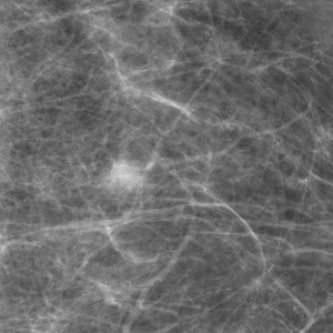
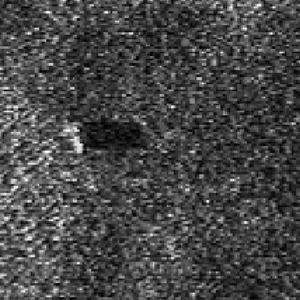
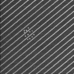
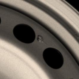
Figure 1: Examples of industrial images with anomalies to detect. From left to right a suspicious mammogram Grosjean and Moisan (2009), an undersea mine Mishne and Cohen (2014), a defective textile pattern Tsai and Hsieh (1999) and a defective wheel Tout (2018).

The automatic detection of anomalous structure in arbitrary images is concerned with the problem of finding non-confirming patterns with respect to the image normality. This is a challenging problem in computer vision, since there is no clear and straightforward definition of what is (ab)normal for a given arbitrary image. Automatic anomaly detection has high stakes in industry, remote sensing and medicine (Figure 1). It is crucial to be able to handle automatically massive data to detect for example anomalous masses in mammograms Tarassenko et al. (1995); Grosjean and Moisan (2009), chemical targets in multi-spectral and hyper-spectral satellite images Ashton (1998); Schweizer and Moura (2000); Stein et al. (2002); Du and Kopriva (2008), sea mines in side-scan sonar images Mishne and Cohen (2013), or defects in industrial monitoring applications Zontak and Cohen (2010); Yeh et al. (2010); Tout et al. (2017). This detection may be done using any imaging device from cameras to scanning electron microscopes Carrera et al. (2016).

Our goal here is to review the broad variety of methods that have been proposed for this problem in the realm of image processing. We would like to classify the methods, but also to decide if some arguably general anomaly detection framework emerges from the analysis. This is not obvious: most reviewed methods were designed for a particular application, even if most claim some degree of generality.

Yet, all anomaly detection methods make a general structural assumption on the “normal” background that actually characterizes the method. By combining the most general structural assumptions with statistical detection tools controlling the number of false alarms, we shall converge to a few generic algorithms that seem to generalize or reconcile most methods.

To evaluate our conclusions, we shall compare representatives of the main algorithmic classes on classic and diversified examples. A fair comparison will require completing them when necessary with a common statistical decision threshold.

Plan of the paper.

In the next subsection 1.1, we make a first sketch of definition of the problem, define the main terminology and give the notation for the statistical framework used throughout the paper. Section 1.2 reviews four anterior reviews and discusses their methodology. Section 1.3 circumscribes our field of interest by excluding several related but different questions. In the central Section 2 we propose a classification of the anomaly detectors into five classes depending on the main structural assumption made on the background model. This section contains the description and analysis of about 50 different methods. This analysis raises the question of defining a uniform detection scheme for all background structures. Hence, in Section 3 we incorporate a uniform probabilistic detection threshold to the most relevant methods spotted in Section 2. This enables us in Section 4 to build three comparison protocols for six methods representative of each class. We finally conclude in Section 5.

1.1 Is there a formal generic framework for the problem?

Because of the variety of methods proposed, it is virtually impossible to start with a formal definition of the problem. Nevertheless, this subsection circumscribes it and lists the most important terms and concepts recurring in most papers. Each new term will be indicated in italic.

Our study is limited to image anomalies for obvious experimental reasons: we need a common playground to compare methods. Images have a specific geometric structure and homogeneity which is different from (say) audio or text. For example, causal anomaly detectors based on predictive methods such as autoregressive conditional heteroskedasticity (ARCH) models fall out of our field. (We shall nevertheless study an adaptation of ARCH to anomaly detection in sonar images.)

Like in the overwhelming majority of reviewed papers, we assume that anomalies can be detected in and from a single image, or from an image data set, even if they do contain anomalies. Learning the background or “normal” model from images containing anomalies nevertheless implies that anomalies are small, both in size and proportion to the processed images, as stated for example in Olson et al. (2018):

“We consider the problem of detecting points that are rare within a data set dominated by the presence of ordinary background points.”

Without loss of generality, we shall evaluate the methods on single images. It appears that for the overwhelming majority of considered methods, a single image has enough samples to learn a background model. As a matter of fact, many methods are proceeded locally in the image or in a feature space, which implies that the background model for each detection test is learned only on a well chosen portion of the image or of the samples. Nevertheless for industrial applications, using a fixed database representative of anomaly-free images can help reduce false alarms and computation time, and studied methods can generally be adapted to this scenario. All methods extract vector samples from the images, either hyperspectral pixels generally denoted by $x_{i},x_{j},x_{r}\cdots$, or image patches, namely sub-images of the image $u$ with moderate size, typically from $2\times 2$ to $16\times 16$, generally denoted by $p_{i},p_{j},q_{r},q_{s},\cdots$. The vector samples may be also obtained as a feature vector obtained by a linear transform (e.g. wavelet coefficients) or by a linear or nonlinear coordinate transform such as, PCA, kernel PCA or diffusion maps, or as coordinates in a sparse dictionary. We denote the resulting vector representing a sample by $\tilde{x}_{i},\tilde{y}_{i},\cdots$ or $\tilde{p}_{i},\tilde{q}_{i},\cdots$.

From these samples taken from an image (or from a collection of images), all considered anomaly detection methods estimate (implicitly or explicitly) a background model, also known as model of normal samples. The goal of the background model is to provide for each sample a measure of its rareness. This rarity measure is generally called a saliency map. It requires an empirical threshold to decide which pixels or patches are salient enough to be called anomalies. If the background model is stochastic, a probability of false alarm or p-value can be associated with each sample, under the assumption that it obeys the background model.

The methods will be mainly characterized by the structure of their background model. This model may be global in the image, which means common to all the image samples, but also local in the image (for center-surround anomaly detectors), or global in the sample space (when a global model is given for all samples regardless of their position in the image). The model may remain local in the sample space when the sample’s anomaly is evaluated by comparing it to its neighbors in the patch space or in the space of hyperspectral pixels. When samples are compared locally in the sample space but can be taken from all over the image, the method is often called non-local, though it can actually be local in the sample space.

Many methods proceed to a background subtraction. This operation, which can be performed in many different ways that we will explore, aims at removing from the data all “normal” variations, attributable to the background model, thus enhancing the abnormal ones, that is, the anomalies.

At the end of the game, all methods compute for each sample its distance to the background or saliency. This distance must be larger than a given value (threshold) to decide if the sample is anomalous. The detection threshold may be empirical, but is preferably obtained through a statistical argument. To explicit the formalism, we shall now detail a classic method.

Du and Zhang (2011) proposed to learn a Gaussian background model from randomly picked $k$ dimensional image patches in a hyperspectral image. Once this background model $p\sim{\mathcal{N}}\left(\mu,\Sigma\right)$ with mean $\mu$ and covariance matrix $\Sigma$ is obtained, the anomalous $(2\times 2)$ patches are detected using a threshold on their Mahalanobis distance to the background

$$d_{\mathcal{M}}(p_{i}):=\sqrt{(p_{i}-\mu)\Sigma^{-1}(p_{i}-\mu)}.$$

Thresholding the Mahanalobis distance boils down to a simple $\chi^{2}$ test. Indeed, one has $d_{\mathcal{M}}^{2}(p)\sim\chi_{k}^{2}$, meaning that the square of the Mahalanobis distance between $p$ and its expectation obeys a $\chi^{2}$ law with $k$ degrees of freedom. Let us denote by $\chi_{k;1-\alpha}^{2}$ the quantile $1-\alpha$, then

$$\mathbb{P}\left[d_{\mathcal{M}}^{2}(p)\leq\chi_{k;1-\alpha}^{2}\right]=1-\alpha=\mathbb{P}\left[p\in ZT_{\alpha}\right],$$

where $ZT_{\alpha}:=\left\{p\in\mathbb{R}^{k}\mid d_{\mathcal{M}}^{2}(p)\leq\chi_{k;1-\alpha}^{2}\right\}$ is the $\alpha$-tolerance zone. Thus, $\alpha$ is the p-value or probability of false alarm for an anomaly under the Gaussian background problem: If indeed $d_{\mathcal{M}}^{2}(p)>\chi_{k;1-\alpha}^{2}$, then the probability that $p$ belongs the background is lower than $\alpha$.

Yet, thresholding the p-value may lead to many false detections. Indeed, anomaly detectors perform a very large number of tests, as they typically test each pixel. For that reason, Desolneux et al. (2004), Desolneux et al. (2007) pointed out that in image analysis computing a number of false alarms (NFA), also commonly called per family error rate (PFER) is preferable. Assume that the above anomaly test is performed for all $N$ pixels $p_{i}$ of an image. Instead of fixing a p-value for each pixel, it is sound to fix a tolerable number $\alpha$ of false alarms per image. Then the “Bonferroni correction” requires our test on $p$ to be $d_{\mathcal{M}}^{2}(p)>\chi_{k;1-\frac{\alpha}{N}}^{2}$. We then have

$$\mathbb{P} \left(\bigcup_{i=1}^{N}[d_{\mathcal{M}}^{2}(p_{i})>\chi_{k;1-\frac{\alpha}{N}}^{2}]\right)$$

$$\leq \sum_{i=1}^{N}\mathbb{P}\left([d_{\mathcal{M}}^{2}(p_{i})>\chi_{k;1-\frac{\alpha}{N}}^{2}]\right)=N\frac{\alpha}{N}=\alpha,$$

which means that the probability of detecting at least one “false anomaly” in the background is equal to $\alpha$. It is convenient to reformulate this Bonferroni estimate in terms of expectation of the number of false alarms:

$$\mathbb{E} \left[\Sigma_{i=1}^{N}\mathbf{1}_{[d_{\mathcal{M}}^{2}(p_{i})>\chi_{k;1-\frac{\alpha}{N}}^{2}]}\right]$$

$$= \sum_{i=1}^{N}\mathbb{E}\mathbf{1}_{[d_{\mathcal{M}}^{2}(p_{i})>\chi_{k;1-\frac{\alpha}{N}}^{2}]}=N\frac{\alpha}{N}=\alpha$$

where $\mathbf{1}$ denotes the characteristic function equal to 1 if and only if its argument is positive. This means that by fixing a lower threshold equal to $\chi_{k;1-\frac{\alpha}{N}}^{2}$ for the distance $d_{\mathcal{M}}^{2}(p)$, we secure on average $\alpha$ false alarms per image.

We can compare this unilateral test to standard statistical decision terms. The final step of an anomaly detector would be to decide between two assumptions:

• $\mathcal{H}_{0}$: the sample $p$ belongs to the background;

• $\mathcal{H}_{1}$: the sample $p$ is too exceptional under $\mathcal{H}_{0}$ and is therefore an anomaly.

Because no model is at hand for anomalies, $\mathcal{H}_{1}$ boils down to a mere negation of $\mathcal{H}_{0}$. $\mathcal{H}_{1}$ is chosen with a probability of false alarm $\frac{\alpha}{N}$ and therefore with a number of false alarms (NFA) per image equal to $\alpha$. We shall give more examples of NFA computations in Section 3.

1.2 A quick review of reviews

More than 1000 papers in Google scholar contain the key words “anomaly detection” and “image”. The existing review papers proposed a useful classification, but leave open the question of the existence of generic algorithms performing unsupervised anomaly detection on any image. The 2009 review paper by Chandola et al. (2009) on anomaly detection is arguably the most complete review. It considered allegedly all existing techniques and all application fields and reviewed 361 papers. The review establishes a distinction between point anomaly, contextual anomaly, collective anomalies, depending on whether the background is steady or evolving and the anomaly has a larger scale than the initial samples. It also distinguishes between supervised, mildly supervised and unsupervised anomalies. It revises the main objects where anomalies are sought for (images, text, material, machines, networks, health, trading, banking operations, etc.) and lists the preferred techniques in each domain. Then it finally proposes the following classification of all involved techniques.

1. Classification based anomaly detection, e.g., SVM, Neural networks. These techniques train a classifier to distinguish between normal and anomalous data in the given feature space. Classification is either multi-class (normal versus abnormal) or one-class (only trains to detect normality, that is, learns a discriminative boundary around normal data). Among the one-class detection methods we have the Replicator Neural Networks (auto-encoders).

2. Nearest neighbor based anomaly detection. The basic assumption of these methods is that normal data instances occur in dense neighborhoods, while anomalies occur far from their closest neighbors. This can be measured by the distance to the $k^{\text{th}}$ nearest neighbor or as relative density.

3. Clustering based anomaly detection. Normal data instances are assumed to belong to a cluster in the data, while anomalies are defined as those standing far from the centroid of their closest cluster.

4. Statistical anomaly detection. Anomalies are defined as observations unlikely to be generated by the “background” stochastic model. Thus, anomalies occur in the low probability regions of the background model. Here the background models can be: parametric (Gaussian, Gaussian mixture, regression), or non-parametric and built, e.g., by a kernel method.

5. Spectral anomaly detection. The main tool here is principal component analysis (PCA) and its generalizations. Its principle is that an anomaly has deviant coordinates with respect to normal PCA coordinates.

6. Information theoretic anomaly detection. These techniques analyze the information content of a data set using information theoretic measures, such as, the Kolomogorov complexity, the entropy, the relative entropy, among others.

This excellent review is perhaps nevertheless biting off more than it could possibly chew. Indeed, digital materials like sound, text, networks, banking operations, etc. are so different that it was impossible to examine in depth the role of their specific structures for anomaly detection. By focusing on images, we shall have a much focused discussion involving their specific structure yielding natural vector samples (color or hyperspectral, pixels, patches) and specific structures for these samples, such as self-similarity and sparsity.

The above review by Chandola et al. (2009) is fairly well completed by the more recent review by Pimentel et al. (2014). This paper presents a complete survey of novelty detection methods and introduces a classification into five groups.

1. Probabilistic novelty detection. These methods are based on estimating a generative probabilistic model of the data (either parametric or non-parametric).

2. Distance-based methods. These methods rely on a distance metric to define similarity among data points (clustering, nearest-neighbour and self-similar methods are included here).

3. Reconstruction-based methods. These methods seek to model the normal component of the data (background), and the reconstruction error or residual is used to produce an anomaly score.

4. Domain-based methods. They determine the location of the normal data boundary using only the data that lie closest to it, and do not make any assumption about data distribution.

5. Information-theoretic methods. These methods require a measure (information content) that is sensitive enough to detect the effects of anomalous points in the dataset. Anomalous samples, for example, are detected by a local Gaussian model, which starts this list.

Our third reviewed review was devoted to anomaly detection in hyperspectral imagery Matteoli et al. (2010). It completes three previous comparative studies, namely Stein et al. (2002), Hytla et al. (2007) and Matteoli et al. (2007). Matteoli et al. (2010) conclude that most of the techniques try to cope with background non-homogeneity, and attempt to remove it by de-emphasizing the main structures in the image, which we can interpret as background subtraction.

For the same authors, an anomaly can be defined as an observation that deviates in some way from the background clutter. The background itself can be identified from a local neighborhood surrounding the observed pixel, or from a larger portion of the image. They also suggest that the anomalies must be sparse and small to make sense as anomalies. Also, no a-priori knowledge about the target’s spectral signature should be required. The question in hyperspectral imagery therefore is to “find those pixels whose spectrum significantly differs from the background”. We can summarize the findings of this review by examining the five detection techniques that are singled out:

1. Modeling the background as a locally Gaussian model Reed and Yu (1990) and detecting anomalous pixels by their Mahanalobis distance to the local Gaussian model learned from its surrounding at some distance. This famous method is called the RX (Reed-Xiaoli) algorithm.

2. Gaussian-Mixture Model based Anomaly Detectors Stein et al. (2002); Ashton (1998); Hazel (2000); Carlotto (2005). The optimization is done by stochastic expectation minimization Masson and Pieczynski (1993). The detection methodology is similar to the locally Gaussian model, but the main difference is that background modeling becomes global instead of local.

   The technical difficulty raised by this more complex model is the variety of clustering algorithms that can be used Duran and Petrou (2005, 2007), and the thorny question of finding the adequate number of clusters as addressed in Duran et al. (2006) and Penn (2002).

3. The Orthogonal Subspace Projection approach. It performs a background estimation via a projection of pixel samples on their main components after an SVD has been applied to all samples. Subtracting the resulting image amounts to a background subtraction and therefore delivers an image where noise and the anomalies dominate.

4. The kernel RX algorithm Kwon and Nasrabadi (2005) which proceeds by defining a (Gaussian) kernel distance between pixel samples and considering that it represents a Euclidean distance in a higher dimension feature space. (This technique is also proposed in Mercier and Girard-Ardhuin (2006) for oil slick detection.) A local variant of this method Ranney and Soumekh (2006) performs an OSP suppression of the background, defined as one of the four subspaces spanned by the pixels within four neighboring subwindows surrounding the pixel at some distance.

5. Background support region estimation by Support Vector Machine Banerjee et al. (2006). Here the idea is that it is not necessary to model the background, but that the main question is to model its support and to define anomalies as observations away from this support.

Our last reviewed review, by Olson et al. (2018), compares “manifold learning techniques for unsupervised anomaly detection” on simulated and real images. Manifold methods assume that the background samples span a manifold rather than a linear space. Hence PCA might be suboptimal and must be replaced by a nonlinear change of coordinates. The authors of the review consider and three kinds for this change of coordinates:

1. Kernel PCA, introduced by Schölkopf et al. Schölkopf et al. (1998) and adapted to the anomaly detection problem by Hoffmann Hoffmann (2007).

2. The Parzen density estimator, which is actually interpreted as the simplest instance of kernel PCA Parzen (1962); Hoffmann (2007).

3. The diffusion map Coifman and Lafon (2006); Lafon et al. (2006), which in this framework appears as a variant of kernel PCA.

We shall review these techniques in more detail in Section 2. In these methods, the sample manifold $\mathcal{M}$ is structured by a Gaussian “distance”

$$k(x_{j},x_{j})=e^{-\frac{1}{h^{2}}||x_{i}-x_{j}||^{2}}.$$

The methods roughly represent the samples by coordinates computed from the eigenvectors and eigenvalues of the matrix $K=(k(x_{i},x_{j}))_{ij}$. This amounts in all cases to a nonlinear change of coordinates. Then, anomalous samples are detected as falling apart from the manifold. The key parameter $h$ is chosen in the examples so that the isolevel surface of the distance function wraps tightly the inliers.

The review compares the ROC curves of the different methods (PCA, kernel PCA, Parzen, diffusion map) and concludes that small ships on a sea landscape are better detected by kernel PCA. Since the review only compares ROC curves between the different methods, it avoids addressing the detection threshold issue.

Discussion.

The above four highly cited reviews made an excellent job of considering countless papers and proposing a categorization of methods. Nevertheless, their final map of the methods is an exhaustive inventory where methods are distributed according to what they do, rather than to what they assume on background and anomaly. Nevertheless, the Pimentel et al. (2014) review is actually close to classify methods by structural assumptions on the background, and we shall follow this lead. The above reviews do not conclude on a unified statistical decision framework. Thus, while reusing most of their categories, we shall attempt at reorganizing the panorama according to three main questions:

• What is the structural assumption made on the background: in other terms what is “normal”?

• How is the decision measurement computed?

• How is the anomaly detection threshold defined and computed, and what guarantees are met?

Our ideal goal would be to find out the weakest (and therefore most general) structural assumption on normal data, and to apply to it the most rigorous statistical test. In other words, the weaker the assumptions of normality, the more generic the detector will be. Before proceeding to a classification of anomaly detection methods, we shall examine several related questions which share some of their tools with anomaly detection.

1.3 What anomaly detection isn’t

1.3.1 Not a classification problem

Most papers and reviews on anomaly detection agree that multi-class classification techniques like SVM can be discarded, because anomalies are generally not observed in sufficient number and lack statistical coherence. There are exceptions like the recent method introduced by Ding et al. (2014). This paper assumes the disposition of enough anomalous samples to learn classification parameters from the data themselves. Given several datasets with dimensions from 8 to 50 with moderate size (a few hundreds to a few thousand samples), this paper applies classic density estimators to sizable extracts of the normal set (k-means, SVM, Gaussian mixture), then learns the optimal thresholds for each classifier and finally compares the performance of these classifiers.

While in many surface defect detection problems, the defect can be of any shape or color, in some industrial applications known recurrent anomalies are the target of defect detectors. In this case a training database can be produced and the detection algorithm is tuned for the detection of the known defects Jia et al. (2004); Yang et al. (2002); Xie (2008). For example, Soukup and Huber-Mörk (2014) proposed to detect rail defects in a completely supervised manner by training a classical convolutional neural networks on a dataset of photometric stereo images of metal surface defects. Another neural-network based method was proposed by Kumar (2003). This paper on the detection of local fabric defects, first performs a PCA dimension reduction on $7\times 7$ windows followed by the training of a neural network on a base of detects / non-detects, thus again performing two-class classification.

To detect changes on optical or SAR satellite images, many methods compare a pair of temporally close images, or more precisely the subtraction between them in the case of optical images Bruzzone and Prieto (2002); Zanetti et al. (2015); Zanetti and Bruzzone (2018); Liu et al. (2017); Bovolo and Bruzzone (2007); Liu et al. (2015); Thonfeld et al. (2016), or the log-ratio for SAR images Bovolo and Bruzzone (2005); Li et al. (2018); Celik (2010); Jia and Wang (2018). However these methods often work on a pair of images where a change is known to have occurred (such as a forest fire Bruzzone and Prieto (2002); Celik (2010), an earthquake Washaya and Balz (2018); Ferrentino et al. (2018) or a flood Li et al. (2018); Clement et al. (2017)), and thus have an a priori for a two class distribution, which leads to classification techniques.

Conclusions.

1.3.2 More than a saliency measure

A broad related literature exists on saliency measures. They associate to each image a saliency map, which is a scalar positive function that can be visualized as an image where the brighter the pixel, the more salient it is. The goal of automatic saliency measures is to emulate the human perception. Hence saliency measures are often learned from a large set of examples associating with images their average fixation maps by humans. For example, Tavakoli et al. (2011) designed an anomaly detector trained on average human fixation maps learning both the salient parts and their surround vectors as Gaussian vectors. This reduced the problem to a two class Bayesian classification problem.

The main difference with anomaly detectors is that many saliency measures try to mimic the human visual perception and therefore are allowed to introduce semantic prior knowledge related to the perceptual system (e.g., face detectors). This approach works particularly well with deep neural networks because attention maps obtained by gaze trackers can be used as a ground truth for the training step. SALICON by Huang et al. (2015) is one of these deep neural networks architecture achieving state of the art performance.

Saliency measures deliver saliency maps, in contrast to anomaly detectors that are requested to give a binary map of the anomalous regions. We can exclude from our review supervised saliency methods based on learning from humans. Yet we cannot exclude the unsupervised methods that are based, like anomaly detectors, on a structural model of the background. The only difference of such saliency maps with anomaly detectors is that that anomaly detectors would require to add a last thresholding step after the saliency map is computed, to transform it into a binary detection map.

Interesting methods for example assign a saliency score to each tested pixel feature based on the inverse of the histogram bin value to which it belongs. In Riche et al. (2013) a saliency map is obtained by combining 32 multiscale oriented features obtained by filtering the image with oriented Gabor kernels. A weighted combination of the most contrasted channels for each orientation yields a unique multiscale orientation channel $c_{o}(i)$ for each orientation. Then the histograms $h_{o}$ of these channels $c_{o}$ are computed and each pixel $i$ with value $c_{o}(i)$ is given a weight which is roughly inversely proportional to its value $h_{o}(c_{o}(i))$ in the histogram. The same rarity measurement is applied to the colors after PCA. Summing all of these saliency maps one obtains something similar to what is observed with gaze trackers: the salient regions are the most visited.

Similarly, image patches are represented by Borji and Itti (2012) using their coefficients on a patch dictionary learned on natural images. Local and global image patch rarities are considered as two “complementary processes”. Each patch is first represented by a vector of coefficients that linearly reconstruct it from a learned dictionary of patches from natural scenes (“normal” data). Two saliency measures (one local and one global) are calculated and fused to indicate the saliency of each patch. The local saliency is computed as the distinctiveness of a patch from its surrounding patches, while the global saliency is the inverse of a patch’s probability of happening over the entire image. The final saliency map is built by normalizing and fusing local and global saliency maps of all channels from both color systems. (Patch rarity is measured both in RGB and Lab color spaces.)

One can consider the work by Murray et al. (2011), as a faithful representative of the multiscale center-surround saliency methods. Its main idea is to:

• apply a multi-scale multi-orientation wavelet pyramid to the image;

• measure the local wavelet energy for each wavelet channel at each scale and orientation;

• compute a center-surround ratio for this energy;

• obtain in that way wavelet contrast coefficients that have the same spatial multi-scale sampling as the wavelet pyramid itself;

• apply the reverse wavelet pyramid to the contrast coefficients to obtain a saliency map.

This is a typical saliency-only model, for which an adequate detection threshold is again missing.

Conclusions.

Saliency detection methods learned from human gaze tracking are semantic methods that fall off our inquiry. But unsupervised saliency measures deliver a map that only needs to be adequately thresholded to get an anomaly map. They therefore propose mechanisms and background structure assumptions that are relevant for anomaly detection. Conversely, most anomaly detectors also deliver a saliency map before thresholding. The last three generic saliency measures listed are tantalizing. Indeed, they seem to do a very good job of enhancing anomalies by measuring rarity. Notwithstanding, they come with no clear mechanism to transform the saliency map into a probabilistic one that might allow hypothesis testing and eventually statistically motivated detection thresholds.

1.3.3 A sketch of our proposed classification

The anomaly detection problem has been generally handled as a “one-class” classification problem. The 2003 very complete review by Markou and Singh (2003) concluded that most research on anomaly detection was driven by modeling background data distributions, to estimate the probability that test data do not belong to such distributions. Hence the mainstream methods can be classified by their approach to background modeling. Every detection method has to do three things:

1. to model the anomaly-free “background”. This background model may be constructed from samples of various sizes extracted from the given image (or an image database): pixels (e.g. in hyperspectral images), patches, local features (e.g. wavelet coefficients).

2. to define a measure on the observed data evaluating how far its samples are from their background model. Generally, this measure is a probability of false alarm (or even better, as we shall see, an expectation of the number of false alarms) associated with each sample.

3. to define the adequate (empirically or statistically motivated) threshold value on the measure obtained in b).

The structure chosen for the background model appears to us as the most important difference between methods. Hence we shall primarily classify the methods by the assumed structure of their background model, and the way a distance of samples to the background model is computed. Section 3 will then be devoted to the computation of the detection thresholds.

We shall examine in detail five generic structures for the background:

1. the background can be modeled by a probability density function (pdf), which is either parametric, such as, a Gaussian, or a Gaussian mixture, or is obtained by interpolation from samples by a kernel density estimation method; this structure leads to detect anomalies by hypothesis testing on the pdf;

2. the background is globally homogeneous (allowing for a fixed reference image, a global Fourier or a convolutional neural network model generally followed by background subtraction);

3. the background is locally spatially homogeneous (leading to center-surround methods);

4. the background is sparse on a given dictionary or base (leading to variational decomposition models).

5. the background is self-similar (in the non-local sense that for each sample there are other similar samples in the image).

2 Detailed analysis of the main anomaly detection families

The main anomaly detection families can be analyzed from their structural assumptions on the background model. In what follows we present and discuss the five different families that we announced.

2.1 Stochastic background models

The principle of these anomaly detection methods is that anomalies occur in the low probability regions of the background model. The stochastic model can be parametric (Gaussian, Gaussian mixture, regression), or non-parametric. For example in “spectral anomaly detection” as presented by Chandola et al. (2009), an anomaly is defined by having deviant coordinates with respect to normal PCA coordinates. This actually assumes a Gaussian model for the background.

Gaussian background model.

The Gaussian background assumption may expand to image patches. Du and Zhang (2011) proposed to build a Gaussian background model from random $2\times 2$ image patches in a hyperspectral image. Once this background model $(\mu,\Sigma)$ is obtained, the anomalous $(2\times 2)$ patches are detected using a threshold on their Mahalanobis distance to the background Gaussian model. The selection of the image blocks permitting to estimate the Gaussian patch model $(\mu,\Sigma)$ is performed by a RANSAC procedure Fischler and Bolles (1987), picking random patches in the image and excluding progressively the anomalous ones.

Goldman and Cohen (2004), aiming at sea-mine detection, propose a detection scheme that does not rely on a statistical model of the targets. It performs a background estimation in a local feature space of principal components (this again amounts to building a Gaussian model). Then, hypothesis testing is used for the detection of anomalous pixels, namely those with an exceedingly high Mahalanobis distance to the Gaussian distribution (Section 1.1). This detects potentially anomalous pixels, which are thereafter grouped and filtered by morphological operators. This ulterior filter suggests that the first stage may yield many false alarms.

Pdf estimation.

Sonar images have a somewhat specific anisotropic structure that leads to model the background using signal processing methods. For example, in Mousazadeh and Cohen (2014) the authors proposed to adapt an ARCH model, thus obtaining a statistical detection model for anomalies not explained by the non-causal model. This method is similar to the detection of scratches in musical records Oudre (2015).

Cohen et al. (1991) detect fabric defects using a Gaussian Markov Random Fields model. The method computes the likelihood of patches of size $32\times 32$ or $64\times 64$ according to the model learned on a database free of defects. The patches are then classified as anomalous or defect-free thanks to a likelihood ratio test.

Tarassenko et al. (1995) identify abnormal masses in mammograms by assuming that abnormalities are uniformly distributed outside the boundaries of normality (defined using an estimation of the probability density function from training data). If a feature vector falls in a low probability region (using a pre-determined threshold), then this feature vector is considered to be novel. The process to build the background model is complex and involves selecting five local features, equalizing their means and variances to give them the same importance, clustering the data set into four classes, and estimating for each cluster its pdf by a non-parametric method (i.e., Parzen window interpolation). Finally, a feature vector is considered anomalous if it has low probability for each estimated pdf. Such a non-parametric pdf estimate has of course an over-fitting or under-fitting risk, due to the fact that training data are limited.

Gaussian Mixture.

The idea introduced by Xie and Mirmehdi (2007) is to learn a texture model based on Julezs’ texton theory Julesz (1981). The textons are interpreted as image patches following a Gaussian model. Thus a random image patch is assumed to follow a Gaussian mixture model (GMM), which is therefore estimated from exemplar images by the expectation-maximization algorithm (EM). The method works at several scales in a Gaussian pyramid with fixed size patches (actually $5\times 5$). The threshold values for detecting anomalies are learned on a few images without defects in the following way: At each scale, the minimum probability in the GMM over all patches is computed. These probabilities serve as detection thresholds. A patch is then considered anomalous if its probability is lower than the minimum learned on the faultless textures on two consecutive dyadic scales in the Gaussian pyramid. A saliency map is obtained by summing up these consecutive probability excesses. Clearly, this model can be transformed from a saliency map to an anomaly detector by using hypothesis testing on the background Gaussian mixture model. Gaussian mixture modeling has been long classical in hyperspectral imagery Ashton (1998) to detect anomalies. In that case, patches are not needed as each hyperspectral pixel already contains rich multidimensional information.

Gaussian Stationary process.

Grosjean and Moisan (2009) propose a method that models the background image as a Gaussian stationary process, which can also be modeled as the result of the convolution of a white Gaussian noise model with an arbitrary kernel, in other terms a colored noise. This background model is rather restrictive, but it is precise and simple to estimate. The Gaussian model is first estimated. Then the image is filtered either with low-pass filters (to detect global peaks in the texture) or center-surround filters (to detect locally contrasted peaks in the texture). The Gaussian probability density function of each of these filtered images is easily computed. Finally, a probabilistic detection threshold for the filtered images is determined by bounding the NFA as sketched in Section 1.1 (we shall give more details on this computation in Section 3.1.)

Conclusions.

To summarize, in the above methods relying on probabilistic background models, outliers are detected as incoherent with respect to a probability distribution estimated from the input image(s). The anomaly detection threshold is a statistical likelihood test on the learned background model. In all cases, it gives (or could give) a p-value for each detection. So, by tightening the detection thresholds, one can easily control the number of false alarms, as done by Grosjean and Moisan (2009) (see Section 1.1).

2.2 Homogeneous background model

These methods estimate and (generally) subtract the background from the image to get a residual image representation on which detection is eventually performed. We shall examine different ways to do so: by using Fourier modeling, auto-encoder networks, or by subtraction of a smooth or fixed background.

Fourier background model.

Perhaps the most successful background based method is the detection of anomalies in periodic patterns of textile Tsai and Hsieh (1999); Tsai and Huang (2003); Perng et al. (2010). This can be done naturally by cutting specific frequencies in the Fourier domain and thresholding the residual to find the defects. For example Tsai and Hsieh (1999) remove the background by a frequency cutoff. Then a detection threshold using a combination of the mean and the variance of the residual yields a detection map.

Similarly, Tsai and Huang (2003) propose an automatic inspection of defects in randomly textured surfaces which arise in sandpaper, castings, leather, and other industrial materials. The proposed method does not rely on local texture features, but on a background subtraction scheme in Fourier domain. It assumes that the spread of frequency components in the power spectrum space is isotropic, and with a shape that is close to a circle. By finding an adequate radius in the spectrum space, and setting to zero the frequency components outside the selected circle, the periodic, repetitive patterns of statistical textures are removed. In the restored image, the homogeneous regions in the original image get approximately flat, but the defective region is preserved. According to the authors, this leads to convert the defect detection in textures into a simple thresholding problem in non-textured images. This thresholding is done using a statistical process control (SPC) binarization method,

$$f_{b}(x,y)=\begin{cases}255&\text{ if }\mu-k\sigma\leqslant f(x,y)\leqslant\mu+k\sigma\\ 0&\text{ otherwise,}\end{cases}$$

where $k$ is a control parameter, $\mu$ is the residual image average and $\sigma^{2}$ its variance. Regions set to zero are then detected.

Perng et al. (2010) focus on anomaly detection during the production of bolts and nuts. The method starts by creating normalized unwrapped images of the pattern on which the detection is performed. The first step consists in removing the “background” by setting to zero some Fourier coefficients. Indeed, the background pattern being extremely periodic, is almost entirely removed by canceling large Fourier coefficients. The mean $\mu$ and the variance $\sigma^{2}$ of the residual are then computed. This residual is then thresholded using the SPC binarization method of Tsai and Huang (2003).

Aiger and Talbot (2010) propose to learn a Gaussian background Fourier model of the image Fourier phase directly from the input image. The method assumes that only a few sparse defaults are present in the provided image. First a “phase only transform (PHOT)” is applied to the image. The Fourier transform of an image contains all the information of its source inside the modulus of the Fourier coefficients and their phase. The phase is known to contain key positional elements of the image, while the modulus relates more to the image texture, and therefore to its background. To illustrate this fact, RPNs are well known models for a wide class of “microtextures” as explained in Galerne et al. (2011b). A RPN is a random image where the Fourier coefficients have deterministic moduli (identical to the reference texture), but random, uniform, independent phases. Another illustration of the role of phase and modulus is obtained noticing that a Gaussian noise has uniform random phase. The PHOT amounts to invert the Fourier transform of an image after normalizing the Fourier coefficients modulus, thus keeping only the structural information contained in the phase. A local anomaly is expected to have a value in excess compared to the PHOT. Anomalous pixels are therefore detected as peaks of the Mahalanobis distance of their values to the background modelled as Gaussian distributed. Hence, a probability of false alarm can be directly computed in this ideal case. The detection method can be also applied after convolving the PHOT transformed image with a Gaussian, to detect blobs instead of single pixels.

Xie and Guan (2000) introduced a method to detect defects in periodic wafer images. By estimating the periods of the repeating pattern, the method obtains a “golden template” of the patterned wafer image under inspection. No other prior knowledge is required. The estimated defect-free background pattern image is then subtracted to find out possible defects.

Neural-network-based background model.

The general idea is to learn the background model by using a neural network trained on normal data. Under the assumption that the background is homogeneous, the “replicator” neural networks proposed by Hawkins et al. (2002) can be used to learn this model. These networks were introduced in section 1.2.

Perhaps the most important application of anomaly detection in industry is surface defect detection. Iivarinen (2000) proposes an efficient technique to detect defects in surface patterns. A statistical self-organizing map (SOM) is trained on defect-free data, using handpicked features from co-occurrence matrices and texture unit elements. The SOM is then able to separate the anomalies, which are supposed to have a different feature distribution. As can be seen in Xie (2008) which reviews surface defect detection techniques, many surface defect detection methods work similarly. Texture features are selected, and defects are detected as being not well explained by the feature model.

Similarly Chang et al. (2009) presented an unsupervised clustering-based automatic wafer inspection system using self-organizing neural networks. An (2016) proposed to train a variational autoencoder (VAE), and to compute from it an average reconstruction probability, which is a different measure than just looking at the difference between the input and output. Given a new data point, a number of samples are drawn from the trained probabilistic encoder. For each code sample, the probabilistic decoder outputs the corresponding mean and variance parameters. Then, the probability of the original data being generated from a Gaussian distribution having these parameters is calculated. The average probability, named reconstruction probability, among all drawn samples is used as an anomaly score.

Mishne et al. (2017) presented an encoder-decoder deep learning framework for manifold learning. The encoder is constrained to preserve the locality of the points, which improves the approximation power of the embedding. Outliers are detected based on the autoencoder reconstruction error. The work of Schlegl et al. (2017) is in the same direction as using an autoencoder and looking at the norm between the original and the output. A Generative Adversarial Network (GAN) Goodfellow et al. (2014) is trained (generator + discriminator) by using anomalous-free data. Then, given a new test image a representation in latent space is computed (by backpropagation), and the GAN reconstruction is compared to the input. The discriminator cost is then used alongside the representation of the input by the network to find the anomalies. There is, however, no guarantee that the latent representation found would do good for anomaly free examples. Hence, it is not clear why the discriminator cost would detect anomalies.

Smooth or fixed background model.

Many surface defect detectors fall into that category. For example, a common procedure to detect defects in semiconductors is to use a fixed reference clean image and apply some detection procedure to the difference of the observed image and the reference pattern Hiroi et al. (1994); Dom and Brecher (1995); Tsai and Yang (2005b); Shankar and Zhong (2005); Tsai and Yang (2005a). Since for different chips, the probability of defects existing at the same position is very low, one can extract a standard reference image by combining at least three images (by replacing pixels located in defects by the pixels located in the corresponding location of another image)Liu et al. (2010). Similar ideas have been exploited for the detection of defects in patterned fabrics Ngan et al. (2011). In Ngan et al. (2005), nonconforming regions are detected by subtracting a golden reference image and processed in the Wavelet domain.

A very recent and exemplary method to detect anomalies in smooth materials is the one proposed by Tout et al. (2016). In this paper, the authors develop a method for the fully automatic detection of anomalies on wheels surface. First, the wheel image are registered to a fixed position. For each wheel patch in a given position, a linear deterministic background model is designed. Its basis is made of a few low degree polynomials combined with a small number of basis functions learned as the first basis vectors of a PCA applied to exemplar data. The acquisition noise is accurately modeled by a two-parameter Poisson noise. The parameters are easily estimated from the data. The background estimation is a mere projection of each observed patch on the background subspace. The residual, computed as the difference between the input and the projection, can contain only noise-and anomalies. Thus, classic hypothesis testing on the norm of the residual of each patch will yield an automatic detection threshold. This method is clearly adapted to defect detection on smooth surfaces.

Conclusions.

Homogeneous background model based anomaly detection methods are compelling detectors used in a wide variety of applications. They avoid proposing a stochastic model for an often complex background by computing the distance to the background or doing background subtraction. However this simplification comes at a cost: some algorithms are hard to generalize to new applications, and the detection decision mechanism is generally not statistically justified, with the exception of some methods, like Tout et al. (2016).

2.3 Local homogeneity models: center-surround detection.

These methods are often used for creating saliency maps. Their rationale is that anomalies (or saliency) occur as local events contrasting with their surroundings.

In one of the early papers on this topic, Itti et al. (1998) propose to compute a set of center-surround linear filters based on color, orientation and intensity. The filters are chosen to only have positive output values. The resultant maps are normalized by stretching their response so that the max is at a pre-specified value. These positive feature maps are then summed up to produce a final saliency map. Detection is then done on a simple winner-takes-all scheme on the maximum of the response maps. This method is applied in Itti and Koch (2000) to detect vehicles via their saliency in huge natural or urban images. It has also been generalized to video in Mahadevan et al. (2010).

The method was expanded by Gao et al. (2008). The features in this paper are basically the same as those proposed by Itti and Koch (2000), that is, color features, intensity features, and a few orientation filters (Gabor functions, wavelets). This last paper does detection on image and video with center-surround saliency detector. It directly compares its results to those of Itti and Koch (2000) and takes similar features, but works differently with them. In particular it computes center-surround discrimination scores for the features, and puts in doubt the linearity of center-surround filters and the need for computing a (necessarily nonlinear) probability of false alarm in the background model. In fact, they claim Gao et al. (2008):

“In particular, it is hypothesized that, in the absence of high-level goals, the most salient locations of the visual field are those that enable the discrimination between center and surround with smallest expected probability of error.”

The difficulty of center-surround anomaly detection is faced by Honda and Nayar (2001), who introduced a generic method which tentatively works on all types of images. The main idea is to estimate a probability density for sub-regions in an image, conditioned upon the areas surrounding these sub-regions. The estimation method employs independent component analysis and the Karhunen-Loève transform (KLT) to reduce dimensionality and find a compact representation of the region space and its surroundings, with elements as independent as possible. Anomaly is again defined as a subregion with low conditional probability with respect to its surrounding. This is both a coarse grained and complex method.

Schölkopf et al. (2000) and Tax and Duin (2004) extended SVM to the problem of one-class detection (support estimation). The general idea is that by assuming that only a small fraction of the training data consist of anomalies, we can optimize the decision function of a classifier to predict if a point belongs or not to the normal class. The goal is to find the simplest or smallest region that is compatible to observing a given fraction of anomalies in the training set. In Gurram et al. (2012), the authors presented an ensemble-learning anomaly detection approach by optimizing an ensemble of kernel-based one-class classifiers.

Very recently, Ruff et al. (2018) introduced a novel approach to detect anomalies using deep-learning that is inspired in the same ideas. The method, named Deep Support Vector Data Description (Deep SVDD), trains a deep neural network by minimizing the volume of a hypersphere that encloses the network representations of the data.

In the famous Reed-Xiaoli (RX) algorithm Reed and Yu (1990) the pixels of a hyperspectral optical image are assumed to follow a Gaussian non-stationary multivariate random process with a rapidly fluctuating space-varying mean vector and a more slowly space-varying covariance matrix. This “local normal model” for the background pixels is learned from an outer window from which a guard window has been subtracted, as it might contain the anomaly. Then detection is performed by thresholding the Mahanalobis distance of the pixel of interest to the local Gaussian model, as described in Section 1.1. It may be noticed that a previous rough background subtraction is performed by a local demeaning using a sliding window Margalit et al. (1985); Chen and Reed (1987). Matteoli et al. (2010) points out two main limitations of the RX method: first, the difficulty of estimating locally a high dimensional covariance matrix, and second the fact that a local anomaly is not necessarily a global anomaly: an isolated tree in a meadow would be viewed as an anomaly, even if its stands close to a wood of the same trees. Nevertheless, RX remains a leading algorithm and it has even online versions: See, e.g., Fowler and Du (2012) for the successful application of RX after a dimensional reduction by random projections, inspired from compressed sensing.

Conclusions.

Most presented center-surround anomaly detectors produce a saliency map, but as previously mentioned in Section 1.3.2, while saliency detectors are tantalizing since they propose simple and efficient rarity measurements, they provide no detection mechanism (threshold value). Several above reviewed center-surround methods attempt to remedy that. But then, the method becomes quite heavy as it requires estimating a local stochastic model for both the center and surround. Hence we are forced back to two-class classification with fewer samples and a far more complex methodology.

2.4 Sparsity-based background models and its variational implementations

One recent non-parametric trend is to learn a sparse dictionary representing the background (i.e., normality) and to characterize outliers by their non-sparsity.

Margolin et al. (2013) propose a method for building salient maps by a conjunction of pattern distinctness and color distinctness. They claim that for pattern distinctness, patch sparsity is enough to characterize visual saliency. They proceed by:

1. Computing the PCA of all patches (of fixed size –typically $8\times 8$) in the image;

2. Computing the pattern saliency of a patch $p$ as $P(p):=\|p\|_{1}$ where the $l^{1}$ norm is computed on the PCA coordinates.

3. The pattern saliency measure is combined (by multiplication) with a color distinctness measure, that measures the distance of each color super pixel to its closest color cluster. The final map therefore is $D(p):=P(p)C(p)$ where $C(p)$ is the color distinctness.

4. The final result is a product of this saliency map with (roughly) a Gaussian centered in the center of mass of the previous saliency map.

We now look at sparsity models that learn the background model as a dictionary on which “normal” patches would have to be represented by a sparse linear combination of the elements of the dictionary (and anomalous patches tentatively would not). Sparse dictionary learning, popularized by the K-SVD algorithm Aharon et al. (2006) and Rubinstein et al. (2010) and online learning methods Mairal et al. (2009a), has been successful for many signal representation applications and in particular for image representation and denoising Mairal et al. (2009b).

Cong et al. (2011); Zhao et al. (2011) proposed a completely unsupervised sparse coding approach for detecting abnormal events in videos based on online sparse reconstructibility of query signals using a learned event dictionary. These methods are based on the principle that normal video events are more likely to be reconstructible from an event dictionary, whereas unusual events are not.

Li et al. (2015b) introduced a low-rank and sparse tensor representation of hyperspectral imaginary HSI) data based on the observation that the HSI data volume often displays a low-rank structure due to significant correlations in the spectra of neighboring pixels.

The anomaly detector in hyperspectral images proposed by Li et al. (2015a) soundly considers learning a background model and not an anomaly model. Its main contribution is perhaps to justify the use of sparsity to estimate a background model even in the presence of a minority of outliers. This detector belongs to the class of center-surround detectors considered in the previous section. In a neighbour of each pixel deprived of a “guard” central square, a sparse model of the background is learned by orthogonal matching pursuit. It is expected that the vectors of the sparse basis will not contain any anomaly. Thus, the projection of the central pixel on the orthogonal space to this basis should have a norm much higher than the average norm observed in the surround if it is anomalous. The detection threshold is based on the ratio between these two numbers and is not further specified. It might nevertheless use a $\chi^{2}$ model, as the background residual could be modeled as white Gaussian noise.

For Boracchi et al. (2014), the background model is a learned patch dictionary from a database of anomaly-free data. The abnormality of a patch is measured as the Mahalanobis distance to a 2D Gaussian learned on the parameter pairs composed by the $\ell_{1}$ norm of the coefficients and of their reconstruction error. In what follows we detail this method.

Although the method looks general, the initial question addressed by Boracchi et al. (2014) is how to detect anomalies in complex homogeneous textures like microfibers. A model is built as a dictionary $\hat{D}$ learned from all patches $p_{i}$ by minimizing

$$J_{\lambda}(X,D)=\|DX-P\|_{F}^{2}+\lambda\|X\|_{1},$$

where $P$ is the matrix whose columns are the reference patches, the dictionary $D$ is represented as a matrix where the columns are the elements of the dictionary, $X$ is a matrix where the $i$-th column represents the coefficients of patch $p_{i}$ on $D$, and the data-fitting error is measured by the Frobenius norm of the first term. The $\ell_{1}$ norm on $X$ must be understood as the sum of the absolute values of all of its coefficients. Once a minimizer $\hat{D}$ is obtained, the same functional can be used to find a sparse representation $\mathbf{x}$ for each patch $p$ by minimizing

$$J_{\lambda}(\mathbf{x})=\|\hat{D}\mathbf{x}-p\|^{2}+\lambda\|\mathbf{x}\|_{1}.$$

The question then arises: how to decide from this minimization that a patch $p$ is anomalous? The authors propose to associate to each patch the pair of values $\phi(p):=(\|\hat{D}\mathbf{x}-p\|,\|\mathbf{x}\|_{1})$. The first component is a data-fidelity term measuring how well the patch is represented in $\hat{D}$. The second component measures the sparsity (and therefore the adequacy) of this representation. An empirical 2D Gaussian model $(\mu,\Sigma)$ is then estimated for these pairs calculated for all patches in the reference anomalous-free dataset. Under this Gaussian assumption, the normality region can be defined for the patch model by fixing an adequate threshold $\gamma$ on the Mahanalobis distance of samples to this Gaussian model (see section 1.1). According to the authors fixing $\gamma$ is a “suitable question” that we shall address in Section 3.5.

The Boracchi et al. (2014) method is directly related to the sparse texture modeling previously introduced by Elhamifar et al. (2012), where a “row sparsity index” is defined to distinguish outliers in a dataset. The outliers are added to the dictionary. Hence, in any variational sparse decomposition of themselves, they will be used primarily as they cannot be sparsely decomposed over the inlier dictionary. In the words of the authors Elhamifar et al. (2012),

“We use the fact that outliers are often incoherent with respect to the collection of the true data. Hence, an outlier prefers to write itself as an affine combination of itself, while true data points choose points among themselves as representatives as they are more coherent with each other.”

As we saw the  Boracchi et al. (2014) method is extremely well formalized. It was completed in Carrera et al. (2016) by adding a multiscale detection framework measuring the anomaly’s non-sparsity at several scales. The 2015 variant by Carrera et al. (2015) of the above models introduces the tempting idea of building a convolutional sparse dictionary. This is done by minimizing

$$L(\textbf{x}_{m},d_{m})=\\ \sum_{p\in\mathcal{P}}\left(\left\|\sum_{m=1}^{M}d_{m}\ast\mathbf{x}_{m}-p\right\|^{2}+\lambda\sum_{m=1}^{M}\|\mathbf{x}_{m}\|_{1}\right),$$

subject to $\|d_{m}\|_{2}=1$, $m=1,\cdots,M$, where $(d_{m})_{m}$ and $(\mathbf{x}_{m})_{m}$ denote a collection of $M$ filters and $M$ coefficient vectors respectively. As usual in such sparse dictionary models, the minimization can be done on both the filters $(d_{m})$ and coordinates $x_{m}$ and summing for a learning set of patches. Deprived of the sum over $p$, the same functional can be minimized for a given input patch $p_{0}$ to compute its coordinates $\textbf{x}_{m}$ and evaluate its sparsity.

Defining anomaly detection as a variational problem, where anomalies are detected as non-sparse, is also the core of the method proposed by Adler et al. (2015). In a nutshell, the $\ell_{1}$ norm of the coefficients on a learned background dictionary is used as an anomaly measure. More precisely, assuming a dictionary $D$ on which normal data would be sparse, the method performs the minimization

$$\min_{X,E}\|Y-DX-E\|_{F}^{2}+\alpha\|X\|_{1,q}+\beta\|E\|_{2,1},$$

where $q=1$ for if sparsity is enforced separately on each sample and $q=2$ for enforcing joint sparsity of all samples and $\|E\|_{2,1}=\sum_{i}\|E(:,i)\|_{2}$ is the $l_{2,1}$ norm. Here $Y$ is the data matrix where each column is a distinct data vector. Similarly $D$ is a matrix whose columns are the dictionary’s components. $X$ is the matrix of coefficients of these data vectors on $D$ which is forced by the $\|X\|_{1,q}$ term to become sparse. Yet anomalies, which are not sparse on $D$, make a residual whose norm is measured as $\|E\|_{2,1}$, therefore their number should be moderated. Of course this functional depending on two parameters $(\alpha,\beta)$ raises the question of their adequate values. The final result is a decomposition $Y\simeq DX+E$ where the difference between $Y$ and $DX+E$ should be mainly noise and therefore we can write this

$$Y=DX+E+N$$

where $N$ is the noisy residual, $DX$ the sparse part of $Y$ and $E$ its anomalies.

In appendix A we prove that the dual variational method amounts to finding directly the anomalies. Furthermore, we have seen that these methods cleverly solve the decision problem by applying very simple hypothesis testing to the low dimensional variables formed by the values of the terms of the functional. Hence, the method is generic, applicable to all images and can be completed by computing a number of false alarms, as we shall see. Indeed, we interpret the apparent over-detection by a neglect of the multiple testing. This can be fixed by the a-contrario method and we shall do it in Section 3.5.

Dual interpretation of sparsity models.

Sparsity based variational methods lack the direct interpretation enjoyed by other methods as to the proper definition of an anomaly. By reviewing the first simplest method of this kind proposed by Boracchi et al. (2014), we shall see that its dual interpretation points to the detection of the most deviant anomaly. Let $D$ a dictionary representing “normal” patches. Given a new patch $p$ we compute the representation using the dictionary,

$$\hat{x}=\operatorname*{arg\,min}_{x}\left\{\frac{1}{2}\|p-Dx\|_{2}^{2}+\lambda\|x\|_{1}\right\},$$

and then build the “normal” component of the patch as $D\hat{x}$.

One can derive the following Lagrangian dual formulation (see Appendix A),

$$\hat{\eta}=\operatorname*{arg\,min}_{\eta}\left\{\frac{1}{2}\|p-\eta\|_{2}^{2}+\lambda^{\prime}\|D^{T}\eta\|_{\infty}\right\},$$ (1)

where the vector $\eta$ are the Lagrangian multipliers.

While $D\hat{x}$ represents the “normal” part of the patch $p$, $\hat{\eta}$ represents the anomaly. Indeed, the condition $\|D^{T}\eta\|_{\infty}\leq\lambda$ imposes to $\eta$ to be far from the patches represented by $D$. Moreover, for a solution $\eta^{*}$ of the dual to exist (and so that the duality gap doesn’t exist) it requires that $\eta^{*}=p-Dx^{*}$ i.e. $p=Dx^{*}+\eta^{*}$ which confirms the previous observation. Notice that the solution of (1) exists by an obvious compactness argument and is unique by the strict convexity of the dual functional.

Conclusions.

The great advantage of the background models assuming sparsity is that they make a very general structural assumption on the background, and derive a variational model that depends on one or two parameters only, namely the relative weights given to the terms of the energy to be minimized.

2.5 Non-local self-similar background models

The non-local self-similarity principle is invoked as a qualitative regularity prior in many image restoration methods, and particularly for image denoising methods such as the bilateral filter Tomasi and Manduchi (1998) or non-local means Buades et al. (2005). It was first introduced for texture synthesis in the pioneering work of Efros and Leung (1999).

The basic assumption of this generic background model, applicable to most images, is that in normal data, each image patch belongs to a dense cluster in the image’s patch space. Anomalies instead occur far from their closest neighbors. This definition of an anomaly can be implemented by clustering the image patches (anomalies being detected as far away from the centroid of their own cluster), or by a nearest neighbor search (NNS) leading to a direct rarity measurement.

As several anomaly detectors derive from NL-means Buades et al. (2005), we shall here give a short overview of this image denoising algorithm. For each patch $p$ in the input image $u$, the $n$ most similar patches denoted by $p_{i}$ are searched and averaged to produce a self-similar estimate,

$$\hat{p}=\frac{1}{Z}\sum_{i=1}^{n}\exp\left(-\frac{\|p-p_{i}\|_{2}^{2}}{h^{2}}\right)p_{i}$$ (2)

where $Z=\sum_{i=1}^{n}\exp\left(-\frac{\|p-p_{i}\|_{2}^{2}}{h^{2}}\right)$ is a normalizing constant, and $h$ is a parameter (which should be set according to the noise estimation) and $\hat{p}$ is the denoised patch.

NL-means inspired model.

An example of anomaly detector with non-local self-similar background model is Seo and Milanfar (2009), Seo and Milanfar propose to directly measure rarity as an inverse function of resemblance. At each pixel $i$ a descriptor $F_{i}$ measures the likeness of a pixel (or voxel) to its surroundings. Then, this descriptor $F_{i}$ is compared to the corresponding descriptors of the pixels in a wider neighborhood. The saliency at a pixel $i$ is measured by

$$S_{i}=\frac{1}{\sum_{j=1}^{N}\exp\left(\frac{\rho(F_{i},F_{j})-1}{h^{2}}\right)},$$ (3)

where $\rho(\cdot,\cdot)$ is the cosine distance between two descriptors, $F_{i}$ is the local feature, and $F_{j}$ for $j=1,\ldots,N$, the $N$ closest features to $F_{i}$ in the surrounding, and $0<h<1$ is a parameter.

The formula reads as follows: if all $F_{j}$ are not aligned to $F_{i}$, the exponentials in (3) will be all small and therefore the saliency will be high. If instead only one $F_{j}$ correlates well with $F_{i}$, the saliency will be close to one, and if $k$ different $F_{j}$s correlate well with $F_{i}$, $S_{i}$ will be approximately equal to $\frac{1}{k}$. This method cannot yield better than a saliency measure, as no clear way of having a detection mechanism emerges: how do we set a detection threshold?

The algorithm in Zontak and Cohen (2010) is closely inspired from NL-means: For a reference patch $p$, a similarity parameter $h^{2}$ and a set of $n$ neighboring patches $(p_{i})$, an anomaly is detected when

$$\sum_{j=1}^{n}e^{\frac{-\|p-p_{j}\|_{2}^{2}}{h^{2}}}\leqslant\tau$$

where $\tau$ is an empirical parameter. The anomaly detection is applied to strongly self-similar wafers, and the authors also display the difference between their actual denoised source image by the NL-means denoising algorithm, and an equally denoised reference image. We can interpret the displayed experiments, if not the method, as a form of background subtraction followed by a detection threshold on the residual. In section 3.4 we shall propose a statistical method for fixing $\tau$.

A similar idea was proposed by Tax and Duin (1998):

“The distance of the new object and its nearest neighbor in the training set is found and the distance of this nearest neighbor and its nearest neighbor in the training set is also found. The quotient between the first and the second distance is taken as indication of the novelty of the object.”

As demonstrated more recently by the SIFT method Lowe (1999) this ratio is a powerful tool. In SIFT a descriptor in a first image is compared to all other descriptors in a target image. If the ratio of distances between the closest descriptor and the second closest one is below a certain threshold, the match between both descriptors is considered meaningful. Otherwise, it is considered casual.

In Davy et al. (2018) the authors of the present review addressed this last step. They proposed to perform background modeling on the residual image obtained by background subtraction. As for the above mentioned self-similarity based methods, the background is assumed self-similar. Thus, to remove it, a variant of the NL-means algorithm is applied. The background modeling consists in replacing each image patch by an average of the most similar ones. These similar patches are found outside a “guard region” centered at the query patch. This precaution is taken to prevent anomalies with some self-similar structure to be kept in the background.

Equation (2) used to reconstruct the background is the same as for NL-means. Since each pixel belongs to several different patches, it receives several distinct estimates that can be averaged to give the final background image $\hat{u}$. Finally, the residual image is built as $r(u)=\hat{u}-u$. Anomalies, having no similarities in the image, should remain in the residual $r(u)$. In the absence of the anomalies, the residual should instead be unstructured and therefore akin to a noise. Then, the method uses the Grosjean and Moisan (2009) a-contrario method to detect fine scale anomalies on the residual. A pyramid of images is used to detect anomalies at all scales. The method is shown to deliver similar results when producing the residual from features obtained from convolutional neural networks instead of the raw RGB features (see Davy et al. (2018)). Still, there is something unsatisfactory in the method: it assumes like Grosjean and Moisan (2009) that the background is an uniform Gaussian random field, but no evidence is given that the residual would obey such a model.

Boracchi and Roveri (2014) proposed to detect structural changes in time-series by exploiting the self-similarity. Their general idea is that a normal patch should have at least one very similar patch along the sequence. Given a temporal patch (a small temporal window) the residual with respect to the most similar patch in the sequence is computed. This leads to a new residual sequence (i.e., change indicator sequence). The final step is to apply a traditional change detector test (CDT) on the residual sequence. CDTs are statistical tests to detect structural changes in sequences, that is, when the monitored data no longer conform to the independent and identical distributed initial model. CDTs run in an online and sequential fashion. The very recent method Napoletano et al. (2018) is similar to the above commented Boracchi and Roveri (2014). Its main difference is the usage of convolutional neural network features instead of image patches.

Kernel PCA background model.

Manifold and PCA kernel methods reduce the computational expense by a uniform random sampling of a small fraction of the data, which has high chance of being uncontaminated by anomalies. The kernel PCA method for anomaly detection introduced by Hoffmann (2007) defines a Gaussian kernel on the dataset $x_{i}$, $i=1,\ldots,M$ by setting $k(x_{i},x_{j})=e^{-\frac{1}{h^{2}}||x_{i}-x_{j}||^{2}}$, $i,j=1,\ldots,M$. This “kernel” is actually assumed to represent the actual scalar product between feature vectors of the samples $\Phi(x_{i})$ and $\Phi(x_{j})$ in a high-dimensional feature space ($\Phi$ being implicitly defined). The trick of kernel PCA consists in performing implicitly a PCA in this feature space with computations only involving $k$. It is possible to compute the distance between $\Phi(z)$ and $\Phi_{0}=\sum_{i=1}^{M}\Phi(x_{i})$ using only $k$:

$$p(z)=k(z,z)-\frac{2}{M}\sum_{i=1}^{M}k(z,x_{i})+\frac{1}{M^{2}}\sum_{i,j=1}^{M}k(x_{i},x_{j}).$$

Since the first term is 1 and the last term constant, it follows that

$$p(z)=C-\frac{2}{M}\sum_{i=1}^{M}k(z,x_{i}),$$

which is opposite to the Parzen density estimation of the sample set using a Gaussian kernel with standard deviation $h$. Thus, anomalies will be detected by setting a threshold on this density computed from the background samples. A more complete background subtraction can be performed by subtracting its $q$ first PCA components.

Diffusion map background model Olson et al. (2018).

The diffusion map construction Coifman and Lafon (2006) views the data as a graph where a kernel function $k(x_{i},x_{j})$ measures vertex similarity. Like in kernel PCA, consider the matrix $K_{ij}=e^{-\frac{1}{h^{2}}||x_{i}-x_{j}||^{2}}$ associated with a Gaussian kernel, and transform it into a probability matrix by setting $p_{ij}=\frac{K_{ij}}{\sum_{j}K_{ij}}$. This matrix is interpreted as the probability that a random walker will jump from $x_{i}$ to $x_{j}$. The probability for a random walk in the graph moving from $x_{i}$ to $x_{j}$ in $t$ time steps is given by $(P^{t})_{ij}$, where $P=(p_{ij})_{ij}$. The eigenvalues $\lambda_{k}$, and eigenvectors $\alpha^{k}$ of the $t$-th transition matrix provide diffusion map coordinates. Using these coordinates one can easily computes the distance (called diffusion distance) between two graph nodes. A background manifold is learned from these samples. Unsampled data are the projected on a local plane tangent to the manifold. The projection error can be then used as an anomaly detection statistic. The distance of a new sample $\theta^{\prime}$ from the manifold is approximated by selecting a subset of $k$ nearest neighbors on the manifold, finding the best least-squares plane through those points, and approximating the distance of the new point from the plane. An adequately threshold on this distance is all that is needed to detect anomalies. We refer to Madar et al. (2011) for an actually very complex anomaly detector based on a diffusion map of an image’s hyperspectral pixels.

More recently, the self-similarity measurement proposed by Goferman et al. (2012), finds for each $7\times 7$ patch $p_{i}$ its $K=64$ most similar patches $q_{k}$ in a spatial neighborhood, and computes its saliency as

$$S_{i}=1-\exp{\left(-\frac{1}{K}\sum_{k=1}^{K}d(p_{i},q_{k})\right)}.$$ (4)

The distance between patches is a combination of Euclidean distance of color maps in LAB coordinates and of the Euclidean distances of patch positions,

$$d(p_{i},p_{j})=\frac{\|p_{i}-p_{j}\|}{1+3\|i-j\|},$$ (5)

where the norm is the Euclidean distance between patch color vectors or between patch positions $p_{i},p_{j}$.

The algorithm computes saliency measures at four different scales and then averages them to produce the final patch saliency. This is a rough measure: all the images are scaled to the same size of 250 pixels (largest dimension) and take patches of size $7\times 7$. The four scales are 100%, 80%, 50% and 30%. A pixel is considered salient if its saliency value exceeds a certain threshold ($S=0.8$ in the examples shown in the paper).

The patch distance (5) used in Goferman et al. (2012) is almost identical to the descriptor distance proposed by Mishne and Cohen (2014). Like in their previous paper Mishne and Cohen (2013), the authors perform first a dimension reduction of the patches. To that aim a nearest neighbor graph on the set of patches is built, where the weights on the edges between patches are decreasing functions of their Euclidean distances, $w(p_{i},p_{j})=\exp\left(-\frac{\|p_{i}-p_{j}\|^{2}}{h^{2}}\right)$. These positive weights allow to define a graph Laplacian. Then the basis of eigenvectors of the Laplacian is computed. The first coordinates of each patch on this basis yield a low dimensional embedding of the patch space. (There is an equivalence between this representation of patches and the application to the patches of the NL-means algorithm, as pointed out in Singer et al. (2009).)

The anomaly score involves the distance of each patch to the first $K$ nearest neighbors, using the new patch coordinates $\tilde{p}_{i}$. This yields the following anomaly score for a given patch $p_{i}$ with coordinates $\tilde{p}_{i}$:

$$S_{i}=1-\exp\left(-\frac{1}{K}\sum_{k=1}^{K}\frac{\|p_{i}-p_{j}\|/2h}{1+c\|\tilde{p}_{i}-\tilde{p}_{j}\|}\right).$$

Note the intentional similarity of this formula with (4) and (5). Mishne and Cohen indeed state that they are adapting the Goferman score to the embedding space. Similar methods have been developed for video Boiman and Irani (2007).

All of the mentioned methods so far have no clear specification of their anomaly threshold. This comes from the fact that the self-similarity principle is merely qualitative. It does not fix a rule to decide if two patches are alike or not.

Conclusions on self-similarity.

Like sparsity, self-similarity is a powerful qualitative model, but we have pointed out that in all of its applications except one, it lacks a rigorous mechanism to fix an anomaly detection threshold. The only exception is Davy et al. (2018), extending the Grosjean and Moisan (2009) method and therefore obtaining a rigorous detection threshold under the assumption that the residual image is a Gaussian random field. The fact that the residual is more akin to a random noise than the background image is believable, but not formalized.

2.6 Conclusions, selection of the methods, and their synthesis

Background category	Background sub-category	Reviewed methods
Stochastic	Gaussian	Du and Zhang (2011); Goldman and Cohen (2004)
	Non-parametric pdf	Mousazadeh and Cohen (2014); Cohen et al. (1991); Tarassenko et al. (1995)
	Gaussian mixture	Xie and Mirmehdi (2007); Ashton (1998)
	Gaussian stationary process	Grosjean and Moisan (2009)
Homogeneous	Fourier	Tsai and Hsieh (1999); Tsai and Huang (2003); Perng et al. (2010); Aiger and Talbot (2010); Xie and Guan (2000)
	Neural-network	Hawkins et al. (2002); Iivarinen (2000); Chang et al. (2009); An (2016); Mishne et al. (2017); Schlegl et al. (2017)
	Smooth/fixed	Hiroi et al. (1994); Dom and Brecher (1995); Tsai and Yang (2005b); Shankar and Zhong (2005); Tsai and Yang (2005a); Liu et al. (2010); Ngan et al. (2005); Tout et al. (2016)
Locally Homogeneous		Itti et al. (1998); Itti and Koch (2000); Gao et al. (2008); Honda and Nayar (2001); Mahadevan et al. (2010); Gurram et al. (2012); Ruff et al. (2018); Reed and Yu (1990); Margalit et al. (1985); Chen and Reed (1987); Fowler and Du (2012)
Sparsity based		Margolin et al. (2013); Cong et al. (2011); Zhao et al. (2011); Li et al. (2015b, a); Boracchi et al. (2014); Elhamifar et al. (2012); Carrera et al. (2015, 2016); Adler et al. (2015)
Non-local self-similar	NL-means inspired	Seo and Milanfar (2009); Zontak and Cohen (2010); Tax and Duin (1998); Davy et al. (2018); Boracchi and Roveri (2014); Napoletano et al. (2018)
	Kernel PCA	Hoffmann (2007)
	Diffusion maps	Olson et al. (2018); Coifman and Lafon (2006); Madar et al. (2011); Goferman et al. (2012); Mishne and Cohen (2013, 2014); Boiman and Irani (2007)

Table 1: Synopsis of the examined anomaly detectors.

Table 1 recapitulates the analyzed papers in Section 2. We observed that the methods giving a stochastic background model are powerful when the images belong to a restricted class of homogeneous objects, like textiles or smooth painted surfaces. Indeed, the method furnishes rigorous detection thresholds based on the estimated probability density function. But, regrettably, stochastic background modeling is not applicable on generic images. For the same reason, homogeneous background models are restrictive and do not rely on provable detection thresholds. We saw that center-surround methods are successful for saliency enhancement, but generally again lack a detection mechanism. We also saw that the center-surround methods proposing a detection threshold have to estimate two stochastic models, one for the center and one for the surround, being therefore quite complex and coarse grained. The last two categories, namely the sparsity and the self-similarity models are tempting and thriving. Their big advantage is their universality: they can be applied to all background images, homogeneous or not, stochastic or not. But again, the self-similarity model lacks a rigorous detection mechanism, because it works on a feature space that is not easily modeled. Nevertheless, several sparsity models that we examined do propose a hypothesis testing method based on a pair of parameters derived from the variational method. But these parameters have no justifiable model and anyway do not take into account the multiple testing. This last objection can be fixed though, by computing a number of false alarms as proposed in Grosjean and Moisan (2009), and we shall do it in the next section.

As pointed out in Davy et al. (2018), abandoning the goal of building a stochastic background model does not imply abandoning the idea of a well-founded probabilistic threshold. Their work hints that background subtraction is a powerful way to get rid of the hard constraint to model background and to work only on the residual. But in Davy et al. (2018) no final argument is given demonstrating that the residual can be modeled as a simple noise. Nevertheless, this paper shows that the parametric Grosjean and Moisan (2009) detection works better on the residual than on the original image (see Section 3.2).

We noticed that at least one paper (Aiger and Talbot (2010)) has proposed a form of background whitening. It seems therefore advisable to improve background subtracting methods by applying the PHOT to the residual. This post-processing step will remove the potential background leftovers of the NL-means inspired background subtracting method, and thus slightly enhance the detection results.

Our conclusion is that we might be closer to a fully generic anomaly detection by combining the best advances that we have listed. To summarize we see two different combinations of these advances that might give a competitive result:

1. The sparsity method joined by an a-contrario decision:

   • model the background by a sparse dictionary Carrera et al. (2016);

   • estimate a Gaussian on the distance parameters (these are actually statistics on the residual) Carrera et al. (2015);

   • apply the a-contrario detection framework on this estimated Gaussian to control the NFA Desolneux et al. (2007).

2. Background subtraction by self-similarity and residual whitening

   • apply a variant of NL-means (using patches from the whole image) excluding a local search region to define the background;

   • obtain the residual by subtracting the background Davy et al. (2018);

   • whiten the residual by the phase only transform (PHOT) Aiger and Talbot (2010);

   • apply the Grosjean and Moisan (2009) center-surround detection criteria to the whitened residual.

These two proposals have the advantage of taking into account all the advances in anomaly detection that we pointed out. They cannot be united; sparsity and self-similarity are akin but different regularity models. We notice that both methods actually work on a residual. In the second proposed method the residual is computed explicitly. In the first one, the decision method is taken on a Gaussian model for a pair of parameters where one is actually the norm of the residual and the other one a sparsity measure. In Section 3 we develop the tools necessary to compare the selected methods. We need a unified anomaly detection criterion, and we shall see that the a-contrario framework, introduced in Section 3.1, gives one.

3 Estimating a number of false alarms for all compared methods

In Section 2, we classified anomaly detection methods into several families based on their background models: stochastic, homogeneous, local homogeneous, sparsity-based and non-local self-similar models. Our final goal is to compare the results of these families by selecting state of the art representatives for each family.

All methods presented in section 2 require a detection threshold. These thresholds are not always explicit and remain empirical in many papers: instead of a universal threshold, most methods propose a range from which to choose depending on the application or even on the image.

To perform a fair comparison of the selected methods, we must automatically set their detection threshold, based on an uniform criterion. This will done by computing for each method a Number of False Alarms, using the a-contrario framework introduced by Desolneux et al. (2004), Desolneux et al. (2007). This detection criterion is already used in two of the examined papers, Grosjean and Moisan (2009) and Davy et al. (2018). We give in the next section a general framework to the explanations given in section 1.1 on the particular example of the Mahanalobis distance.

3.1 Computing a number of false alarms in the a-contrario framework

The a-contrario framework is classical in many detection or estimation computer vision tasks, such as line segment detection Von Gioi et al. (2010); Grompone von Gioi et al. (2012), ellipse detection Patraucean et al. (2012), spot detection Grosjean and Moisan (2009), vanishing points detection Lezama et al. (2014, 2017), fundamental matrix estimation Moisan and Stival (2004), image registration Moisan et al. (2012), mirror-symmetry detection Patraucean et al. (2013), cloud detection Dagobert (2017), among others.

The a-contrario framework is a general methodology to automatically fix a detection threshold in terms of hypothesis testing. This is done by linking the number of false alarms (NFA) and the probability of false alarm, typically used in hypothesis testing. It relies on the following simple definition.

Definition 1

Grosjean and Moisan (2009) Given a set of random variables $(X_{i})_{i\in[1,N]}$ with known distribution under a null-hypothesis $(\mathcal{H}_{0})$, a test function $f$ is called an NFA if it guarantees a bound on the expectation of its number of false alarms under $(\mathcal{H}_{0})$, namely:

$$\forall{\varepsilon>0},\mathbb{E}[\#\{i,f(i,X_{i})\leq\varepsilon\}]\leq\varepsilon.$$

To put it in words, raising a detection every time the test function is below $\varepsilon$ should give under $(\mathcal{H}_{0})$ an expectation of less than $\varepsilon$ false alarms. An observation $\mathbf{x}_{i}$ is said to be “$\varepsilon$-meaningful” if it satisfies $f(i,\mathbf{x_{i}})\leq\varepsilon$, where $\varepsilon$ is the predefined target for the expected number of false alarms. The lower $f(i,\mathbf{x})$ the “stronger” the detection.

Notice that the function $f(i,X_{i})$ is called an NFA function but we call also its value for a given sample an NFA. Thus we can use expressions like “the NFA of $X_{i}$ is lower than $\varepsilon$”.

While the definition of the background model $(\mathcal{H}_{0})$ doesn’t contain any a priori information on what should be detected, the design of the test function $f$ reflects expectations on what is an anomaly. A common way to build an NFA is to take

$$f(i,\mathbf{x_{i}})=N\mathbb{P}_{\mathcal{H}_{0}}(X_{i}\geq\mathbf{x}_{i})$$ (6)

or

$$f(i,\mathbf{x_{i}})=N\mathbb{P}_{\mathcal{H}_{0}}(|X_{i}|\geq|\mathbf{x}_{i}|),$$ (7)

where $N$ is the number of tests, $i$ goes over all tests, and $\mathbf{x}_{i}$, are the observations which excess should raise an alarm. These test functions are typically used when anomalies are expected to have higher values than the background in the first case, or when anomalies are expected to have higher modulus than the background. If for example the $(X_{i})$ represent the pixels of an image, there would be one test per pixel and per channel. Hence $N$ would be the product of the image dimension by the number of image channels.

Grosjean and Moisan (2009) proved that the test function (6) satisfies Definition 1. Since the only requirement of their proof is that $X_{i}$ has to be a real-valued random variable, a more general result can be derived for any function $g$ and multi-dimensional $X_{i}$ if $g(X_{i})$ is a real-valued random variable. Under these conditions, the following function

$$f(i,\mathbf{x})=N\mathbb{P}_{\mathcal{H}_{0}}(g(X_{i})\geq g(\mathbf{x}_{i}))$$ (8)

also is a NFA.

In short, applying the a-contrario framework just requires a stochastic background model $(\mathcal{H}_{0})$ giving the laws of the random variables $X_{i}$, and a test function $f$.

In Davy et al. (2018) for example, $X_{i}$ denote the pixels of the residual image $r(u)$, that presumably follow a Gaussian colored noise model. This Gaussian model defines the null hypothesis $(\mathcal{H}_{0}$), and $N$ is the total number of tested pixels (considering all the scales and channels), and the test function is given by (7).

Proposition 1

Consider the simplest case where all tested variables are equally distributed under $(\mathcal{H}_{0})$, and assume that their cumulative distribution function is invertible. Assume that the test function is given by (7). Then testing if $|\mathbf{x}_{i}|$ is above $\gamma_{\varepsilon}$ defined by

$$\mathbb{P}(|X|\geq\gamma_{\varepsilon})=\frac{\varepsilon}{N}$$ (9)

ensures a number of false alarms lower that $\varepsilon$.

In the particular a-contrario setting given by Eq. (9), the number of false alarms gives a result similar to the Bonferroni correction Bland and Altman (1995), used to compensate for multiple testing. It is also interpretable as a per family error rate Hochberg and Tamhane (1987). Deeper results can be found in Desolneux et al. (2007).

In the next sections we specify the a-contrario framework for the methods that we will be comparing.

3.2 The Grosjean and Moisan (2009) stochastic parametric background model and the Davy et al. (2018) self-similarity model

Grosjean and Moisan (2009) proposed to model the input image as a colored Gaussian stationary process. The method is designed to detect bright local spots in textured images, for example, mammograms. Three different ways to compute a NFA are proposed by locally assuming (i) no context, (ii) contrast related to the context, and (iii) a conditional context. Method (i) comes down to convolving the image with disk kernels, and testing the tails of the obtained Gaussian distributions, while method (ii) comes down to convolving with center-surround kernels. Their second method is preferred since with strong noise correlation the local average in their background model can be far from 0.

In Davy et al. (2018), a residual image is produced with a self-similarity removal step, which contains a normalization step to make the noise more Gaussian. The residual is then supposed to behave as colored Gaussian noise. Then the method comes down to convolving the residual with disk kernels, and testing the tails of the obtained Gaussian distributions.

Both methods do combine the detection at several scales of the input image. Thus, both methods share a similar detection mechanism and can be expressed in the same terms. Under their $(\mathcal{H}_{0})$, the result of the convolutions of the image for the former, and of the residual for the latter, with the testing kernels are colored Gaussian noise which mean and variance can be estimated accurately from the filtered image itself. Hence, the NFA test function applied on all the residual values (pixel/channel/residual) is exactly the function (7). Both methods assume the anomaly impact on the variance estimation is negligible (small anomaly).

3.3 The Fourier homogeneous background model of Aiger and Talbot (2010)

In the Aiger and Talbot (2010) method, a residual is obtained by setting the value of the modulus of the Fourier coefficients of the image (PHOT) to 1. The residual is then modeled a-contrario as a simple Gaussian white noise whose mean and variance are estimated from the image. Anomalous pixels are therefore detected by using a threshold on the Mahalanobis distance between the pixel value and the background Gaussian model. Let $(\mathcal{H}_{0})$ be the null hypothesis under which the residual values $(X_{i})$ follow a Gaussian distribution with mean $\mu$ and variance $\sigma^{2}$. Then we have

$$\mathbb{P}\left(\left|\frac{X_{i}-\mu}{\sigma}\right|\geqslant\gamma_{\varepsilon}\right) =2\int_{\gamma_{\varepsilon}}^{\infty}\frac{e^{-\frac{u^{2}}{2}}}{\sqrt{2\pi}}du$$ (10)

$$={\text{erfc}}\left(\frac{\gamma_{\varepsilon}}{\sqrt{2}}\right).$$ (11)

Thus, the associated function

$$f(i,\mathbf{x}_{i})=N\mathbb{P}\left(\left|\frac{X_{i}-\mu}{\sigma}\right|\geqslant\left|\frac{\mathbf{x}_{i}-\mu}{\sigma}\right|\right)$$

is an NFA of the form (8), where the number of tests $N$ corresponds to the number of pixels in the image. This NFA leads to detect an anomalous pixel when $\left|\frac{\mathbf{x}_{i}-\mu}{\sigma}\right|$ is above $\gamma_{\varepsilon}$ verifying

$$\gamma_{\varepsilon}:=\sqrt{2}{\text{erfc}}^{-1}\left(\frac{\varepsilon}{N}\right).$$

The impact of anomalies impact on the PHOT is assumed to be negligible, which implicitly assumes small or low intensity anomalies with respect to the background.

3.4 The Zontak and Cohen (2010) non-local self-similar model

In this method, the detection test is based on the NL-means weights. If the sum of these weights is smaller than a threshold $\tau$ (before normalization of these weights), then it is considered an anomaly. In what follows, we discuss how to choose this threshold $\tau$ by computing a NFA. We restrict ourselves to the case where the distance between patches is the $\ell_{2}$ distance.

Let us recall that for a reference patch $p$, a similarity parameter $h^{2}$ and a set of $n$ neighboring patches $(p_{i})$, an anomaly is detected when

$$\sum_{j=1}^{n}e^{\frac{-\|p-p_{j}\|_{2}^{2}}{h^{2}}}\leqslant\tau.$$ (12)

Under $(\mathcal{H}_{0})$, every patch $X_{i}$ of the image is associated with $n$ spatially close patches $P_{i,j}$. At least one of these patches is similar and only differs by the realization of the noise, the noise-free content assumed to be identical. The noise is supposed to be for each pixel an independent centered Gaussian noise of variance $\sigma^{2}$. We know that

$$f(i,\mathbf{x})=N\mathbb{P}\left(\sum_{j=1}^{n}e^{\frac{-\|X_{i}-P_{i,j}\|_{2}^{2}}{h^{2}}}\leqslant\sum_{j=1}^{n}e^{\frac{-\|\mathbf{x}_{i}-p_{i,j}\|_{2}^{2}}{h^{2}}}\right),$$ (13)

verifies the NFA property (this is just equation (8) with a well chosen $g$).

By hypothesis, at least one of the $P_{i,j}$ - we shall name $P_{i}^{*}$ one of these patches - is a realization of the same content than $X_{i}$ but with different noise (that we suppose to be of standard deviation $\sigma$).

By event inclusion,

$$\mathbb{P}\left(\sum_{j=1}^{n}e^{\frac{-\|X_{i}-P_{i,j}\|_{2}^{2}}{h^{2}}}\leqslant\tau\right)\leqslant\mathbb{P}\left(e^{\frac{-\|X_{i}-P_{i}^{*}\|_{2}^{2}}{h^{2}}}\leqslant\tau\right).$$

Moreover

$$\mathbb{P}\left(e^{\frac{-\|X_{i}-P_{i}^{*}\|_{2}^{2}}{h^{2}}}\leqslant\tau\right)=\mathbb{P}\left(\frac{\|X_{i}-P_{i}^{*}\|_{2}^{2}}{h^{2}}\geqslant-\log(\tau)\right)\\ =1-\mathbb{P}\left(\frac{\|X_{i}-P_{i}^{*}\|_{2}^{2}}{2\sigma^{2}}\leqslant-\frac{h^{2}}{2\sigma^{2}}\log(\tau)\right).$$

Here we suppose that the candidate is indeed the same as the patch modulo the noise. Therefore the distance follows a $\chi^{2}$ law of degree the size of the patch.

That is,

$$\mathbb{P}\left(e^{\frac{-\|X_{i}-P_{i}^{*}\|_{2}^{2}}{h^{2}}}\leqslant\tau\right)=1-\text{chi2}\left(-\frac{h^{2}}{2\sigma^{2}}\log(\tau)\right)$$

where chi2 is the cumulative density function of the $\chi^{2}$ distribution of the degree the size of the patch.

Thus, by bounding (13) from above, and using the fact that a function whose value is always above a NFA is also a NFA (there will be fewer or an equal number of detections), the following test function also is a NFA:

Thus, by definition of a NFA, a detection is raised if

$$f(i,\mathbf{x})\leqslant\varepsilon,$$

which leads to a threshold $\tau_{\varepsilon}$ on $\sum_{j=1}^{n}e^{\frac{-\|\mathbf{x}_{i}-p_{i,j}\|_{2}^{2}}{h^{2}}}$ satisfying

$$\tau_{\varepsilon}:=\exp\left(-\frac{2\sigma^{2}}{h^{2}}\text{chi2inv}\left(1-\frac{\varepsilon}{N}\right)\right).$$

In order to fit the $(\mathcal{H}_{0})$ hypothesis we can estimate $\sigma^{2}$ using Ponomarenko et al. (2007) noise level estimation, in the implementation proposed by Colom and Buades (2013).

3.5 The Boracchi et al. (2014) sparsity-based background model

In this method the detection is done using a threshold on the Mahalanobis distance. Chen (2007) has shown, as a generalization of Chebyshev’s inequality, that for a random vector $X$ of dimension $d$ with covariance matrix $C$ we have

$$\mathbb{P}((X-\mathbb{E}(X))^{T}C^{-1}(X-\mathbb{E}(X))\geqslant\gamma)\leqslant\frac{d}{\gamma},$$

Moreover, it has been shown in Navarro (2014) that this inequality is sharp if no other assumptions are made on $X$. Therefore, in the case of this method, for a candidate $X_{i}$ and a reference set $P$,

$$\mathbb{P}(d_{\mathcal{M}}(X_{i})\geqslant\gamma)\leqslant\frac{2}{\gamma^{2}},$$ (14)

where the Mahalanobis distance $d_{\mathcal{M}}(\cdot)$ is computed with respect to the empirical mean and covariance of the set $P$. Hence, the function

$$f(i,\mathbf{x})=N\mathbb{P}(d_{\mathcal{M}}(X_{i})\geqslant d_{\mathcal{M}}(\mathbf{x}_{i}))$$

is clearly an NFA associated to the method. Using (14) and the obvious fact that a function whose value is always above an NFA also is an NFA, we deduce that the test function

$$f(i,\mathbf{x})=\frac{2N}{d_{\mathcal{M}}(\mathbf{x}_{i})^{2}}$$

also is a NFA. Thus, a detection is made if

$$\frac{2N}{d_{\mathcal{M}}(\mathbf{x}_{i})^{2}}\leqslant\varepsilon,$$

which leads to a threshold $\gamma_{\varepsilon}$, such that

$$d_{\mathcal{M}}(\mathbf{x}_{i})\geqslant\gamma_{\varepsilon}:=\sqrt{\frac{2N}{\varepsilon}}.$$

While the method was originally presented as using an external database of anomaly free detections, we use it on the image itself i.e. the dictionary is learned on the image, under the assumption that it presents too few anomalies to disturb the dictionary.

3.6 The Mishne and Cohen (2014) non-local self-similar model

There is no obvious way to formalize this method under the a-contrario framework. For the experiments that we present in Section 4, we use the detection threshold suggested in the original paper even though there is no actual theoretical justification.

4 Experiments

In this section we shall compare the six methods analyzed in Section 3. In what follows, we detail the different variants that we finally compare:

• The Grosjean and Moisan (2009) stochastic parametric background model as explained in Section 3.2. The NFA computation has been adapted to take into account both tails of a pixel’s distribution, with tests performed on all pixels. We denote this method by Grosjean.

• The Aiger and Talbot (2010) Fourier homogeneous model using the a-contrario detection threshold as specified in Section 3.3. We denote this method by Aiger.

• The Zontak and Cohen (2010) non-local self-similar model using the a-contrario detection threshold as specified in Section 3.4. We denote this method by Zontak.

• The sparsity-based background model of Boracchi et al. (2014) using the a-contrario detection threshold as specified in Section 3.5. We denote this method by Boracchi.

• The non-local self-similar model of Mishne and Cohen (2014) with the detection threshold as detailed in the original publication. We denote this method by Mishne.

• The non-local self-similar model of Davy et al. (2018) where the phase only transform (PHOT) is applied before the distribution normalization. The NFA is computed as explained in Section 3.2. We denote this method by Davy.

We propose two types of experimental comparison.

• The first comparison is a qualitative sanity check. For this qualitative analysis we tested on synthetic examples having obvious anomalies of different types (color, shape, cluster), or inexistent (white noise). These toy examples provide a sanity check since one would expect all algorithms to perform perfectly on them. We will also examine the results of the competitors on challenging examples taken from anomaly detection articles.

• The second protocol is a quantitative evaluation. We generated anomaly-free images as samples of colored random Gaussian noise. Being a spatially homogeneous random process, such images should remain neutral for an anomaly detector. We then introduced small anomalies to these images and evaluated whether these synthetic anomalies were detected by the competitors. This leads to evaluate a true positive detection rate (TP) for each method on these images. We also evaluated how much of the anomaly free background was wrongly detected, namely the false positive detection rate (FP). Disposing of TP-FP pairs yields ROC curves that will be opportunely discussed. Undoubtedly, the colored Gaussian noise used in this experiment could be replaced by any other spatially homogeneous random process. We varied the background texture by varying strongly the process’s power spectrum.

4.1 Qualitative evaluation

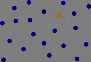
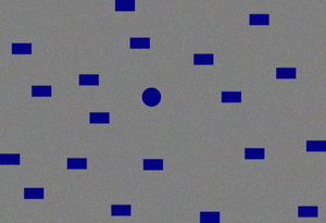
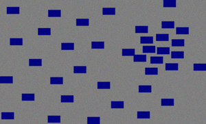
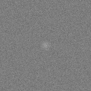
A[residual Davy et al. (2018)

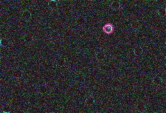
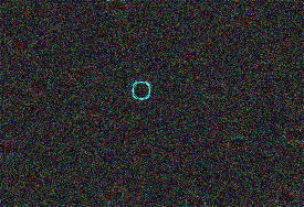
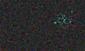
A[ Davy Davy et al. (2018)

A[Aiger Aiger and Talbot (2010)

A[Zontak Zontak and Cohen (2010)

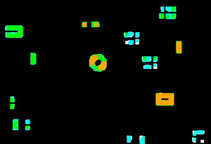
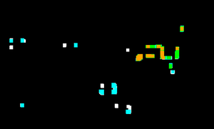
A[Mishne Mishne and Cohen (2014)

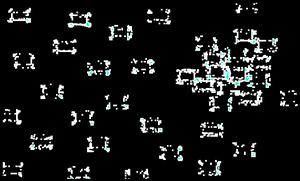
A[Grosjean Grosjean and Moisan (2009)

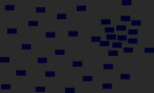
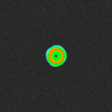
A[Boracchi Boracchi et al. (2014)

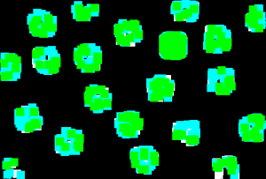
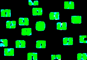
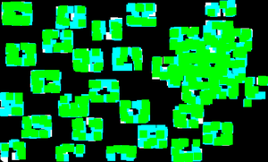
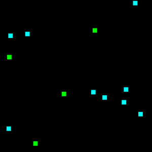
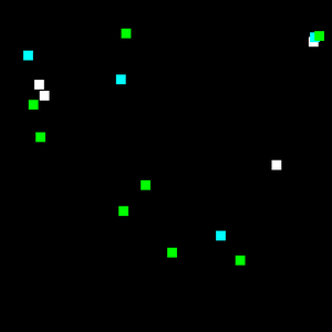
Figure 6: From left to right: Image presenting an anomaly in colors, in shape and in density, image of pure noise, and image of noise with an anomaly in the middle (from Grosjean and Moisan (2009)). From top to bottom: The original image, the image residual of one of the scales computed in Davy et al. (2018) (the scale shown is the one where the anomaly is the most salient, the contrast has been adjusted for visualization purpose), algorithm detections for: Davy et al. (2018), Aiger and Talbot (2010), Zontak and Cohen (2010), Mishne and Cohen (2014), Grosjean and Moisan (2009) and Boracchi et al. (2014). Detections are shown using the following color coding: white is a weak detection - threshold with NFA $\in[10^{-3},10^{-2}]$, cyan is a mild detection - threshold with NFA $\in[10^{-8},10^{-3}]$, green is a strong detection - threshold with NFA $\in[10^{-21},10^{-8}]$, and orange is very strong - threshold with NFA $\leq 10^{-21}$. When available, red is the detection with the threshold corresponding to the lowest NFA. For Mishne and Cohen (2014) we adopted a similar color coding: white between $0$ and $0.5$, cyan between $0.5$ and $0.7$, green between $0.7$ and $0.9$ and orange above $0.9$.

The toy examples are probably the easiest to analyze. We show the results in Figure 6. We generated images in the classic form used in anomaly detection benchmarks like in Riche et al. (2013), where the anomaly is the shape or the color that is unique in the figure. In the third toy example most rectangles are well spaced except in a small region. The anomaly therefore is a change in spatial density. Even though these examples are extremely simple to analyze, they appear to challenge several methods, as can be seen in Figure 6. Only Davy et al. (2018) is able to detect accurately the anomaly in all three examples. This is explained in the second row where the residual after background subtraction is shown. In the residual details of the anomalies stand out on a noise-like background. While Aiger and Talbot (2010) works well with the color and the shape, it fails to detect the spatial density anomaly. Zontak and Cohen (2010) detects well but also lots of false detection. The other methods Zontak and Cohen (2010); Mishne and Cohen (2014); Grosjean and Moisan (2009) and Boracchi et al. (2014) over-detect the contours of the non anomalous shapes, thus leading to many false positives. We also tried a sanity check with a pure white Gaussian noise image. This is done in the last two examples of Figure 6. Davy et al. (2018), and Grosjean and Moisan (2009) soundly detect no anomaly in white noise, as expected. However a few detections are made by Boracchi et al. (2014) and almost everything is detected by Mishne and Cohen (2014). It can be noted that the background model of the first three papers is directly respected in the case of white Gaussian noise, which explains the perfect result. (In the case of the model of Davy et al. (2018), it has to be noted that non-local means asymptotically transforms white Gaussian noise into white Gaussian noise Buades et al. (2008)). The over-detection in Mishne and Cohen (2014) can be explained by the lack of an automatic statistical threshold. The few spurious detections in Boracchi et al. (2014) show that the feature used for the detection doesn’t follow a Gaussian distribution, contrarily to the method’s testing assumption. It is also clear that one cannot build a sound sparse dictionary for white noise.

The same test was done after adding a small anomalous spot to the noise, and the conclusion is similar: Davy et al. (2018); Grosjean and Moisan (2009) perform well, Boracchi et al. (2014) has a couple of false detections and doesn’t detect the anomaly. One method, Zontak and Cohen (2010), doesn’t detect anything. Finally Mishne and Cohen (2014) over-detects. Both noise images were taken from Grosjean and Moisan (2009).

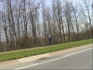
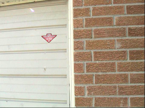
A[residual Davy et al. (2018)

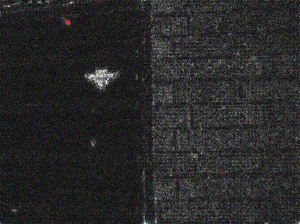
A[Davy Davy et al. (2018)

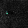
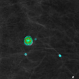
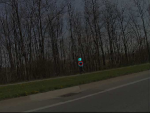
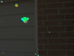
A[Aiger Aiger and Talbot (2010)

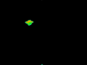
A[Zontak Zontak and Cohen (2010)

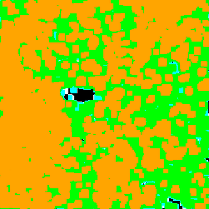
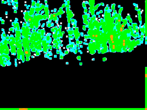
A[Mishne Mishne and Cohen (2014)

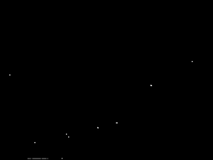
A[Grosjean Grosjean and Moisan (2009)

A[Boracchi Boracchi et al. (2014)

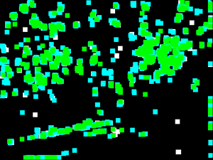
Figure 7: From left to right: image of an undersea mine from Mishne and Cohen (2014), image of a periodic textile from Tsai and Hsieh (1999), image of a tumor from Grosjean and Moisan (2009), image of a man from the Toronto dataset Bruce and Tsotsos (2006), image of a garage door from Bruce and Tsotsos (2006). From top to bottom: The original image, the image residual of one of the scales computed in Davy et al. (2018) (the scale shown is the one where the anomaly is the most salient, the contrast has been adjusted for visualization purpose), algorithm detections for: Davy et al. (2018), Aiger and Talbot (2010), Zontak and Cohen (2010), Mishne and Cohen (2014), Grosjean and Moisan (2009) and Boracchi et al. (2014). Detections are shown using the following color coding: white is a weak detection - threshold with NFA $\in[10^{-3},10^{-2}]$, cyan is a mild detection - threshold with NFA $\in[10^{-8},10^{-3}]$, green is a strong detection - threshold with NFA $\in[10^{-21},10^{-8}]$, and orange is very strong - threshold with NFA $\leq 10^{-21}$. When available red is the detection with the threshold corresponding to the lowest NFA. For Mishne and Cohen (2014) we adopted a similar color coding: white between $0$ and $0.5$, cyan between $0.5$ and $0.7$, green between $0.7$ and $0.9$ and orange above $0.9$.

We then analyze three examples coming from previous papers. The first one (first column in Figure 7) is a radar image of an undersea mine borrowed from Mishne and Cohen (2014). The mine is detected by Davy et al. (2018); Grosjean and Moisan (2009) without any false detections. Both Mishne and Cohen (2014); Boracchi et al. (2014) have false detections; Zontak and Cohen (2010) over-detects and Aiger and Talbot (2010) misses the mine. The second example (second column in Figure 6) shows an example of near-periodic texture. This is one of the examples where Fourier based methods are ideally well suited. It was therefore important to check if more generic methods were still able to detect the anomaly. Two methods Aiger and Talbot (2010) and Grosjean and Moisan (2009) fail to detect the anomaly, the other three methods performing really well. This makes the case for self-similarity and sparsity based methods, that generalize nicely the background’s periodicity assumption. The final example (third column from Figure 7) is a real example of medical imaging borrowed from Grosjean and Moisan (2009) where the goal is to detect the tumor (the large white region). Aiger and Talbot (2010); Boracchi et al. (2014) fail to detect the tumor. A strong detection is given by Zontak and Cohen (2010); Mishne and Cohen (2014) but the false alarms are also strong and numerous. Finally Davy et al. (2018) has stronger tumor detections than Grosjean and Moisan (2009)) (a NFA of $10^{-6.6}$ against $10^{-2.8}$) but it has several false alarms as well.

Finally we tested the methods on real photographs taken from the Toronto dataset Bruce and Tsotsos (2006). This clearly takes several of the methods out of their specific context and type of images (tumors in X-ray images, mine detection in sonar scans, clot detection in microfibers, wafer defects,…) On the other hand, the principles of the algorithms are general. So by testing on these examples, our goal is to explore the limits of several detection principles, not to compare these specific algorithms. Clearly some of the methods are more adapted for spatially homogeneous background than to an outdoor cluttered scene.

Another issue when using real photographs is that anomalies detected by humans may be semantic. None of the methods we consider was made to detect semantic anomalies, that can only be learned on human annotated images. Nevertheless, the tests’ results are still enlightening. Detections are very different from one method to the other. The fourth example in Figure 7 shows a man walking in front of some trees. Aiger and Talbot (2010); Grosjean and Moisan (2009) and Mishne and Cohen (2014) don’t detect anything. Both Zontak and Cohen (2010); Boracchi et al. (2014) detect mostly the trees and the transition between the road and the sidewalk. Surprisingly Davy et al. (2018) only detects the man. Indeed in the noise like residual one can check that the man stands out. The second example shows a garage door as well as a brick wall. This time the algorithms tend to agree more. The conspicuous sign on the door is well detected by all methods as well the lens flare. A gap at the bottom between the brick wall and the door is detected by Davy et al. (2018); Mishne and Cohen (2014); Grosjean and Moisan (2009); Boracchi et al. (2014). The methods Mishne and Cohen (2014) and Boracchi et al. (2014) also detect the transition between the wall and and the brick wall. Finally some detections on the brick wall are made by Davy et al. (2018) and Boracchi et al. (2014). The residuals of Davy et al. (2018) on the second row are much closer to noise than the background, which amply justify the interest of detecting on the residual rather than on the background. Nevertheless, the residual has no reason to be uniform, as is apparent in the garage’s residual. Even if the detections look any way acceptable, this non-uniformity of the residual noise suggests that center-surround detectors based on a local variance (as done in Grosjean and Moisan (2009)) might eventually be preferable.

Fixing a target number of $10^{-2}$ for the NFA means that under the $(\mathcal{H}_{0})$ model, only $10^{-2}$ false positives should occur per image. Yet, many of them shown examples show several false positives. Given the mathematical justification of these thresholds, false positives come from discrepancies between the hypothetical $(\mathcal{H}_{0})$ model and the image. In the case of Zontak and Cohen (2010), the over-detection in the trees of the picture with a man can be explained by the limited self-similarity of the trees: for this region, the nearest patches won’t be close enough to the patch to reconstruct to fit the model, which requires at least one would-be-identical-except-for-the-noise patch in the neighborhood. The over-detection in the case of the undersea mine is likely a mismatch of the noise model with the picture noise. The many false alarms of this method for the other examples, makes us wonder if the model hypothesis is not too strong. The Boracchi et al. (2014) method triggers many false detections in almost all examples tested. As we mentioned, this suggests that the Gaussian model for the detection pairs is inaccurate. This is not necessarily a problem for specific fault detection applications where the false alarm curves can be learned.

4.2 Quantitative evaluation

Estimating how well an anomaly detector works “in general” is a challenging evaluation task. Qualitative experiments such as the ones presented in section 4.1 give no final decision. Our goal now is to address the performance evaluation in terms of true positive rate (TP) and false positive rate (FP). To that aim, we generated a set of ten RPN textures Galerne et al. (2011a) which are deprived of any statistical anomalies. We then introduced one artificial anomaly per rpn by merging a small piece of another image inside each of them. This was made by simple blending or by Poisson editing Pérez et al. (2003) using the implementation of Di Martino et al. (2016). This method provides a set of images where a ground truth is known. Hence the detection quality measure can be clearly defined. Figure 2 shows one of the generated RPN images with an anomaly added and the anomaly’s ground truth locus. Table 2 shows the result for our six methods on this dataset.

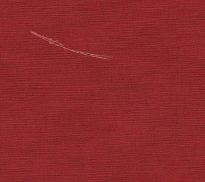
Figure 2: A ground truth (on the right) for anomaly detection has been generated by introducing an anomaly in a RPN Galerne et al. (2011b) texture (on the left), which is anomaly free. The detection is then done on the result (in the middle).

	TP pixels (in %)	FP pixels (in %)	TP anomalies (in %)	FP anomalies (in %)
Aiger and Talbot (2010)	$56.2$	$7.60\times 10^{-4}$	90	40
Zontak and Cohen (2010)	$0$	$0$	0	0
Mishne and Cohen (2014)	$23.4$	$8.52$	90	90
Boracchi et al. (2014)	$78.2$	$0.87$	100	100
Grosjean and Moisan (2009)	$11.6$	$0.16$	30	20
Davy et al. (2018)	$33.1$	$1.79\times 10^{-5}$	80	10

Table 2: Quantitative comparative results for anomaly detection. The number of true positive (TP) and false positive (FP) for different metrics is shown. TP pixels and FP pixels correspond to detections at a pixel level. A true positive is when an anomalous pixel is detected, and a false positive when a normal pixel is detected as anomalous. TP anomalies and FP anomalies evaluate if anomalies have been detected at all. A true positive is counted when there is at least one detected pixel in an anomalous region, and a false positive when there is at least one detection completely outside an anomalous region (with a maximum of 1 FP per image). These results were computed on a dataset of random uniform textures with a single anomaly added to each image. The thresholds were set for a targer number of false alarms (NFA) of $10^{-2}$ per image (theoretical FP pixels of $4\times 10^{-6}\%$). An example of an image from the dataset is shown in Figure 2. A method works correctly if it detects a high percentage of anomalies (third column) while having a good pixel coverage (first column), and a minimal false positive rate (second and fourth columns). Having a very low false positive rate is crucial for massive fault detection. In that sense, the best methods are Aiger and Talbot (2010) and Davy et al. (2018).

	TP pixels (in %)	FP pixels (in %)	TP anomalies (in %)	FP anomalies (in %)
Aiger and Talbot (2010)	$79.1$	$1.0$	100	100
Zontak and Cohen (2010)	$27.2$	$1.0$	60	60
Mishne and Cohen (2014)	$12.5$	$1.0$	50	90
Boracchi et al. (2014)	$80.1$	$1.0$	100	100
Grosjean and Moisan (2009)	$24.2$	$1.0$	70	100
Davy et al. (2018)	$65.0$	$1.0$	100	100

Table 3: This table is similar to Table 2, but in this case each method detection threshold is set so as there are $1\%$ false positives. Hence, the criterion is to detect as many anomalies as possible (third column) while having a high true positive rate. The winners are clearly Boracchi et al. (2014) and Aiger and Talbot (2010).

Table 2 demonstrates that for all methods, the predicted number of false positives (namely the theoretical NFA) is not always achieved. Indeed, the threshold for Table 2 was chosen so that the theoretical number of false detections per image should be $10^{-2}$. When taking into account the total number of pixels, this means that only around $4\times 10^{-6}\%$ false detections should be made by any method in this table. Only two methods are close to this number: Aiger and Talbot (2010) and Davy et al. (2018), while the other compared methods make too many false detections. Such a false positive target might seem too strict. Yet, it is an important requirement of anomaly detectors in fault detection to minimize the false alarm rate. Indeed excessive false alarms may put a production chain in jeopardy. Images are generally of the order of $10^{7}$ pixels. Therefore if one wants to limit the false detection rate in a series of tested images, the false positive rate needs to be really small. The methods compared - except Mishne and Cohen (2014) - used the NFA framework as seen in Section 3. Therefore the discrepancy between the theoretical target and the obtained number of false alarms is explained by an inadequate $(\mathcal{H}_{0})$ for the images. In fact, only the background model of Aiger and Talbot (2010) matches completely these really specific textures that are RPNs.

To better compare the methods, we also computed ROC curves for all methods, Figures 4 and 5, as well as the table of true positive areas and false positive areas for a fixed positive rate of $1\%$ (Table 3). The ROC curve aren’t impacted by the choice of thresholds. Figure 4 is shown with a log scale for the number of false positives because its low or very low false positive section is much more relevant for anomaly detection than the rest. From these ROC curves and tables we can conclude, for this specific example, that Aiger and Talbot (2010) (Area under the curve (AUC) 7.52) (which theoretically should be optimal for this problem) performs the best followed closely by Davy et al. (2018) (AUC 7.03). It’s worth noting that Davy et al. (2018) is performing better than Aiger and Talbot (2010) for very low false positive region. We then have Boracchi et al. (2014) (AUC 5.79). The trailing methods are Grosjean and Moisan (2009) (AUC 3.30), Zontak and Cohen (2010) (AUC 2.92) and finally Mishne and Cohen (2014) (AUC 1.98) . Nevertheless, if a moderate number of false positives can be tolerated, then Boracchi et al. (2014) becomes really attractive because of its high detection precision. Figure 5 illustrates the problem of false detections. Most methods requires many false detections to achieve a reasonable detection rate. Only Aiger and Talbot (2010) (AUC 0.82) and Davy et al. (2018) (AUC 0.87) detect well while still keeping a zero false detection rate. This confirms the results from Table 2. Table 3 also shows that having a $1\%$ detection is useful to obtain a good precision but leads to almost all images getting false positives. In practice $1\%$ is too large a tolerance for images. In Figure 3 we show the result of the detections on 2 corresponding to Table 2 for the different methods.

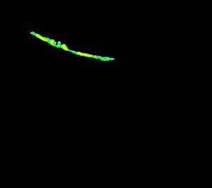
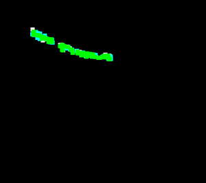
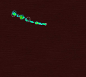
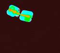
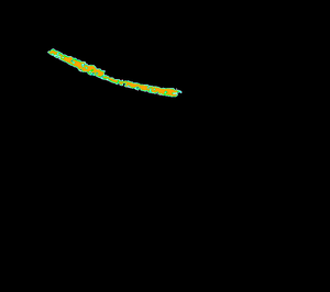
Figure 3: Example of detections for all the different methods on 2. It corresponds to the one showed in Table 2. From left to right: Aiger and Talbot (2010), Boracchi and Roveri (2014), Davy et al. (2018), Grosjean and Moisan (2009), Mishne et al. (2017) and Zontak and Cohen (2010).

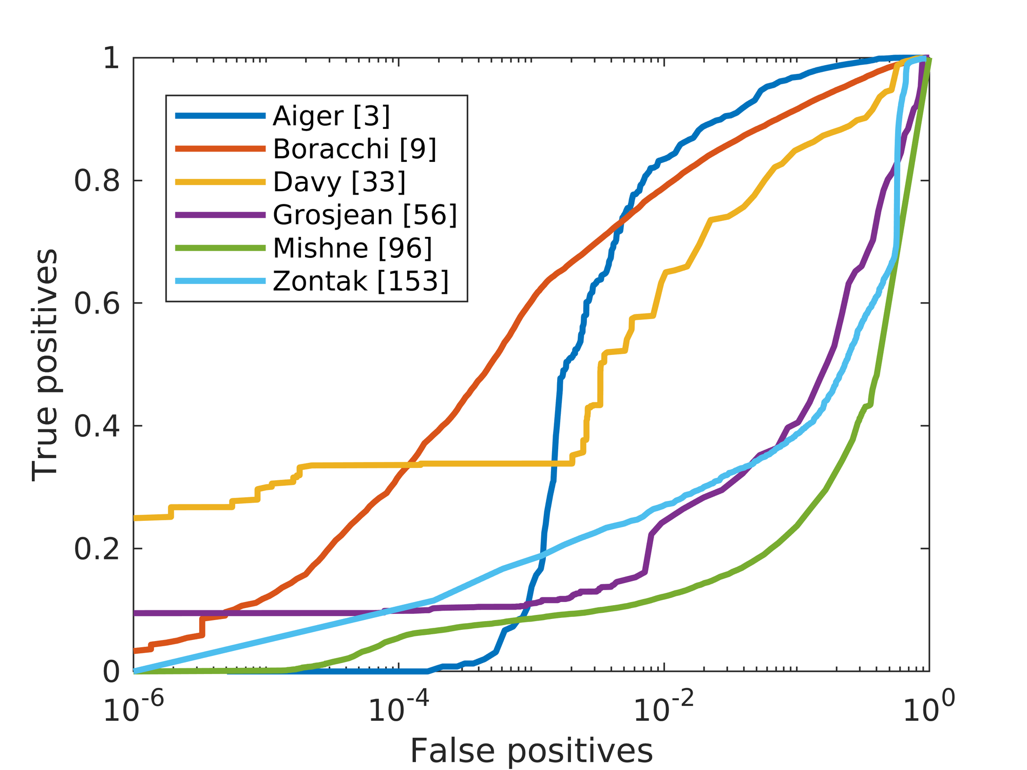
Figure 4: ROC curve computed on the dataset of synthetic images. A true positive corresponds to an anomalous pixel detected. A false positive corresponds to a normal pixel that has been detected as anomalous. In deep blue Aiger and Talbot (2010) (Area Under the Curve (AUC) $7.52$), in red Boracchi et al. (2014) (AUC $5.79$), in yellow Davy et al. (2018) (AUC $7.03$), in purple Grosjean and Moisan (2009) (AUC $3.30$), in green Mishne and Cohen (2014) (AUC $1.98$) and in light blue Zontak and Cohen (2010) (AUC $2.92$).

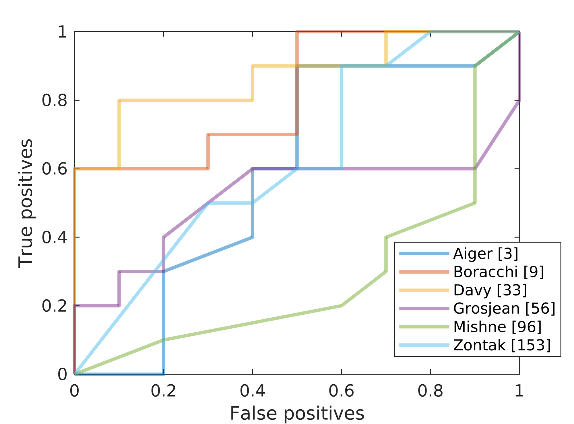
Figure 5: ROC curve computed on the dataset of synthetic images. A true positive is when an anomaly is detected (in the sense that at least one detection has been made inside the anomalous region). A false positive is when there is a detection outside the anomalous region. In deep blue Aiger and Talbot (2010) (Area Under the Curve (AUC) $0.82$), in red Boracchi et al. (2014) (AUC $0.585$), in yellow Davy et al. (2018) (AUC $0.87$), in purple Grosjean and Moisan (2009) (AUC $0.52$), in green Mishne and Cohen (2014) (AUC $0.28$) and in light blue Zontak and Cohen (2010) (AUC $0.625$).

A[input image

A[input image

4.3 Impact of the parameters

Until now we considered the parameters suggested in the corresponding papers. While it can be interesting to fine tune parameters depending on the application we wanted to stay as generic as possible which led us to fix the same parameters for all the experiments, whatever the type of images, for a given method. In this section we show qualitatively that the parameters impact little on the detection results: playing with the parameters neither adds new interesting detections, nor reduces the quantity of false detections. To evaluate that we selected a few images from our qualitative testing set and computed the results with different sets of parameters. The different experiments are presented in Figures 8, 9, 10 and 11. There is actually a non negligible difference for Zontak and Cohen (2010), the reason is probably that the model assumed during the derivation of the NFA is not completely valid. It is also interesting to see that using not too big patches allows to keep a good precision of the detected region. Nevertheless this experiment validates the choice of parameters for the different models, as the detections are not too drastically different for most methods. We specify here the different parameters used for the different methods:

1. Boracchi et al. (2014): $15\times 15$ patches with a redundancy of $1.5$;

2. Davy et al. (2018): $8\times 8$ patches with $16$ nearest neighbors;

3. Mishne et al. (2017): $8\times 8$ patches with $16$ nearest neighbors;

4. Zontak and Cohen (2010): $8\times 8$ patches with a region of size $160\times 160$, we also set $h$ the similarity parameter to the known noise level $\sigma$ as it seems to work best in practice.

A[ $4\times 4$ patches                  $8\times 8$ patches               $16\times 16$ patches               $32\times 32$ patches A[ $4$ neighbors

A[ $8$ neighbors

A[ $16$ neighbors

A[ $32$ neighbors

Figure 8: Impact of parameters for the detection using Davy et al. (2018). The two parameters studied are the size of the patch and the number of patches.

A[ $4\times 4$ patches                  $8\times 8$ patches               $16\times 16$ patches               $32\times 32$ patches A[ $20\times 20$ region

A[ $40\times 40$ region

A[ $80\times 80$ region

A[ $160\times 160$ region

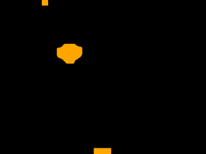
Figure 9: Impact of parameters for the detection using Zontak and Cohen (2010). The two parameters studied are the size of the patch and the size of the region used for the computation.

A[ $8\times 8$ patches               $16\times 16$ patches               $32\times 32$ patches A[ $8$ neighbors

A[ $16$ neighbors

A[ $32$ neighbors

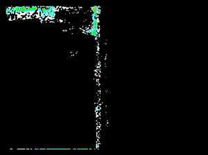
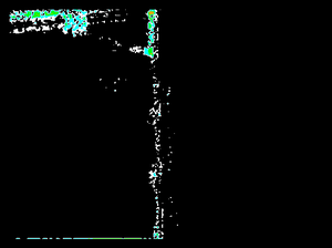
Figure 10: Impact of parameters for the detection using Mishne and Cohen (2014). The two parameters studied are the size of the patch and the number of patches.

A[ $5\times 5$ patches                  $10\times 10$ patches               $15\times 15$ patches               $20\times 20$ patches A[ $1.2\times$ redundancy

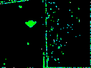
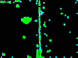
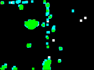
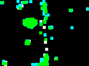
A[ $1.5\times$ redundancy

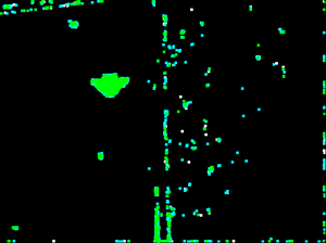
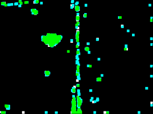
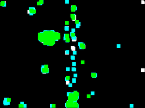
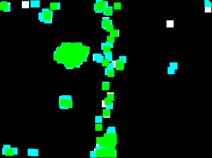
A[ $2\times$ redundancy

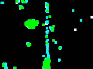
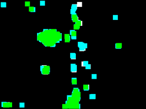
A[ $4\times$ redundancy

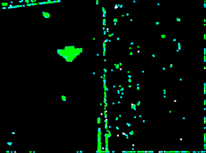
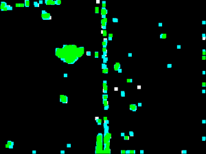
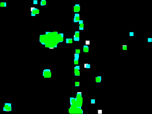
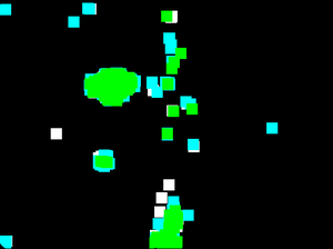
Figure 11: Impact of parameters for the detection using Boracchi et al. (2014). The two parameters studied are the size of the patch and the redundancy of the dictionary.

4.4 Computation time analysis

In this section we do a brief computation time analysis. All algorithms have wildly different computation times. For example Aiger and Talbot (2010) method is really fast as no really complex computations are needed. On the contrary the Mishne and Cohen (2014) method is really slow. Table 4 summarizes the computation time for the different algorithms for the parameter used for the experiment. It’s worth noting that for the larger parameters the Mishne and Cohen (2014) method requires many hours to compute a single result. It’s also worth noting that even though the Boracchi et al. (2014) and Davy et al. (2018) algorithms are not the fastest ones, the dictionaries of patches and indexes for the searches can be precomputed and therefore accelerated for fast industrial applications. For example the processing of Boracchi et al. (2014) only takes 12s when the dictionary is prelearned. The computation time estimation was done on a core i7-7820HQ 2.90GHz using authors’ code whenever it was available (Boracchi et al. (2014), Davy et al. (2018) and Mishne and Cohen (2014) are multithreaded so actual computation times are reported. We report $1/8$ of the actual computation time for Aiger and Talbot (2010), Grosjean and Moisan (2009) and Zontak and Cohen (2010) for a fair comparison).

Aiger and Talbot (2010)	Boracchi et al. (2014)	Davy et al. (2018)	Grosjean and Moisan (2009)	Mishne and Cohen (2014)	Zontak and Cohen (2010)
0.09	1375	57	1.4	749	394

Table 4: Computation time (in seconds) for the different methods reviewed in details with the parameter chosen for the experiments for the door image (size: $600\times 450$.

5 Discussion and conclusions

Our analysis and experiments seem to confirm the view that generic anomaly detection methods can be built on purely qualitative assumptions. Such methods do not require a learning database for the background or the anomalies, but can learn directly normality from a single image in which anomalies may be present. Why not using more images? Certainly disposing of a “golden reference” or even of a database of “golden references” may seem to be ideal situation. But the majority and the best methods succeed to work with a single image. For some methods though, or applications, disposing of a database can help enhance the results and the computation time (by precomputing a dictionary for example). This success of detecting on a single image is of course possible only under the assumption that anomalies are a minor part of the image. Some of the most performing methods use anyway only a small part of the image samples, processing locally in the image domain on in the sample domain. Using the present image also has the advantage of providing an updated background.

Since anomalies cannot be modeled, the focus of attention of all methods is the background model. Methods giving a stochastic model to the background, parametric or not, could only be applied to restricted classes of background. For this reason, our attention has been drawn to the thriving qualitative background models. Any assumption about a kind of global or local background homogeneity is a priori acceptable. The most restrictive models assume that the background is periodic, or smooth or even low dimensional. This kind of strong regularity assumption is not extensible to any image.

Another common sense principle is put forward by local contrast center-surround detectors, which anomalies generate local anomalous contrast. Yet center-surround methods suffer from the difficulty of defining a universal detection rule.

A more clever idea has emerged with the Aiger and Talbot (2010) method, which is to transform the background into a homogeneous texture while the anomalies would still stand out.

Meanwhile the old idea of performing a background subtraction remains quite valid. Indeed, as pointed out still very recently in Tout et al. (2016), background subtraction may be used to return to an elementary background model for the residual that might contain only noise.

The most general background models are merely qualitative. We singled out two of them as the most recent and powerful ones: the sparsity assumption and the self-similarity assumption. We found that two recent exponents use these assumptions to perform a sort of background subtraction: Carrera et al. (2017) for sparsity and Davy et al. (2018) for self-similarity.

We compared methods on various examples in Section 4 and found some methods tend to work better on these various inputs than others, but no method stands out as the best on all images. For applications of anomaly detection, we advise using methods which background model describes the best the expected anomaly-free background, as it will generally lead to the best performance. In our quantitative experiments, Section 4.2, Aiger and Talbot (2010)’s background model was closest to the background of our synthetic examples, and got the best AUC.

Furthermore, we found that all methods required a strict control of the number of false alarms to become universal. Indeed most methods were originally presented with at best an empirical threshold and at worst a comment saying that the threshold depends on the application. The first method proposing this is the one by Grosjean and Moisan (2009), and it was recently extended in Davy et al. (2018). Since Grosjean and Moisan (2009) requires a background stochastic model, we concluded that a good universal model should:

• subtract a background model that is merely qualitative (self-similar, sparse);

• handle the residual as a stochastic process to detect anomalies as anomalies in a colored noise;

• possibly also whiten the residual before detecting the anomaly.

This way, most methods are generalized in a common framework. We tested three such syncretic methods and compared them favorably with the three other most relevant methods taken from the main classes of background models. Our comparative tests were made on very diverse images. Our quantitative comparison tests were made on simulated ground truths with stochastic background.

Both tests seem to validate the possibility of detecting anomalies with very few false alarms using a merely qualitative background model. This fact is both surprising and exciting. It confirms that there has been significant progress in the past decade. We hope that this study, at the very least, provides users with useful generic tools that can be combined for any detection task.

Appendix A Appendix: Dual formulation of sparsity models

Sparsity based variational methods lack the direct interpretation enjoyed by other methods as to the proper definition of an anomaly. By reviewing the first simplest method of this kind proposed in Boracchi et al. (2014), we shall see that its dual interpretation points to the detection of the worst anomaly. Let $D$ a dictionary representing “normal” image patches. For a given patch $p$ the normal patch corresponding to $p$ is $\hat{p}=D\hat{x}$ where

$$\hat{x}=\operatorname*{arg\,min}_{x}\left\{\frac{1}{2}\|p-Dx\|_{2}^{2}+\lambda\|x\|_{1}\right\}.$$

One can derive the following dual optimization problem: Let $z=p-Dx$,

$$\min_{x}\left\{\frac{1}{2}\|z\|_{2}^{2}+\lambda\|x\|_{1}\right\}\text{ s.t }z=p-Dx.$$

The Lagrangian is in this case

$$\mathcal{L}(x,z,\eta) =\frac{1}{2}\|z\|_{2}^{2}+\lambda\|x\|_{1}+\eta^{T}(p-Dx-z)$$

$$=\eta^{T}p+\left(\frac{1}{2}\|z\|_{2}^{2}-\eta^{T}z\right)+(\lambda\|x\|_{1}-\eta^{T}Dx).$$

The dual problem is then

$$\mathcal{G}(\eta) =\inf_{x,z}\mathcal{L}(x,z,\eta)$$

$$=\eta^{T}p+\inf_{z}\left(\frac{1}{2}\|z\|_{2}^{2}-\eta^{T}z\right)+\inf_{x}(\lambda\|x\|_{1}-\eta^{T}Dx).$$

Consider first $\inf_{z}\left(\frac{1}{2}\|z\|_{2}^{2}-\eta^{T}z\right)$: This part is differentiable in $z$ so that

$$\partial_{z}\left(\frac{1}{2}\|z\|_{2}^{2}-\eta^{T}z\right)=z-\eta$$

therefore the inf is achieved for $z=\eta$. The inf is in this case

$$\inf_{z}\left(\frac{1}{2}\|z\|_{2}^{2}-\eta^{T}z\right)=-\frac{1}{2}\|\eta\|_{2}^{2}$$

As for $\inf_{x}(\lambda\|x\|_{1}-\eta^{T}Dx)$: This part is not differentiable (because not smooth) nevertheless the subgradient exists. Let $v$ such that $\|x\|_{1}=v^{T}x$ (for all i $v_{i}\in{-1,1}$). The subgradient of $\|.\|_{1}$ gives $v$.

$$\partial_{x}\left(\lambda\|x\|_{1}-\eta^{T}Dx\right) =\partial_{x}\left(\lambda v^{T}x-\eta^{T}Dx\right)$$

$$=\lambda v-D^{T}\eta$$

A necessary condition to attain the infimum is then $0\in\{\lambda v-D^{T}\eta\}$. This leads to $v=\frac{D^{T}\eta}{\lambda}$ with the condition that $\|D^{T}\eta\|_{\infty}\leq\lambda$ (because $\|v\|_{\infty}\leq 1$) which can be injected into the previous equation which gives

$$\inf_{x}(\lambda\|x\|_{1}-\eta^{T}Dx) =\inf_{x}(\lambda v^{T}x-\eta^{T}Dx)$$

$$=\lambda(\frac{D^{T}\eta}{\lambda})^{T}x-\eta^{T}Dx$$

$$=\eta^{T}Dx-\eta^{T}Dx$$

$$=0$$

Finally,

$$\mathcal{G}(\eta)=\eta^{T}p-\frac{1}{2}\|\eta\|_{2}^{2}$$

Therefore the dual problem is

$$\sup_{\eta}\left\{\eta^{T}p-\frac{1}{2}\|\eta\|_{2}^{2}\right\}\text{ s.t. }\|D^{t}\eta\|_{\infty}\leq\lambda$$

which is equivalent to

$$\sup_{\eta}\left\{-\frac{1}{2}\|p-\eta\|_{2}^{2}\right\}\text{ s.t. }\|D^{t}\eta\|_{\infty}\leq\lambda.$$

It can be reformulated in a penalized version as

$$\hat{\eta}=\operatorname*{arg\,min}_{\eta}\left\{\frac{1}{2}\|p-\eta\|_{2}^{2}+\lambda^{\prime}\|D^{T}\eta\|_{\infty}\right\}.$$ (15)

While $D\hat{x}$ represents the “normal” part of the patch $p$, $\hat{\eta}$ represents the anomaly. Indeed, the condition $\|D^{T}\eta\|_{\infty}\leq\lambda$ imposes to $\eta$ to be far from the patches represented by $D$. Moreover, for a solution $\eta^{*}$ of the dual to exist (and so that the duality gap doesn’t exist) it requires that $\eta^{*}=p-Dx^{*}$ i.e. $p=Dx^{*}+\eta^{*}$ which confirms the previous observation. Notice that the solution of (15) exists by an obvious compactness argument and is unique by the strict convexity of the dual functional.

References

- Adler et al. (2015) Adler, A., Elad, M., Hel-Or, Y., Rivlin, E.: Sparse coding with anomaly detection. Journal of Signal Processing Systems 79(2), 179–188 (2015)
- Aharon et al. (2006) Aharon, M., Elad, M., Bruckstein, A., et al.: K-svd: An algorithm for designing overcomplete dictionaries for sparse representation. IEEE Transactions on signal processing 54(11), 4311 (2006)
- Aiger and Talbot (2010) Aiger, D., Talbot, H.: The phase only transform for unsupervised surface defect detection. In: 2010 IEEE Conference on Computer Vision and Pattern Recognition, pp. 295–302. IEEE (2010)
- An (2016) An, J.: Variational Autoencoder based Anomaly Detection using Reconstruction Probability. Arxiv (2016)
- Ashton (1998) Ashton, E.A.: Detection of subpixel anomalies in multispectral infrared imagery using an adaptive bayesian classifier. IEEE Transactions on Geoscience and Remote Sensing 36(2), 506–517 (1998)
- Banerjee et al. (2006) Banerjee, A., Burlina, P., Diehl, C.: A support vector method for anomaly detection in hyperspectral imagery. IEEE Transactions on Geoscience and Remote Sensing 44(8), 2282–2291 (2006)
- Bland and Altman (1995) Bland, J.M., Altman, D.G.: Multiple significance tests: the bonferroni method. Britsh Medical Journal 310(6973), 170 (1995)
- Boiman and Irani (2007) Boiman, O., Irani, M.: Detecting irregularities in images and in video. International journal of computer vision 74(1), 17–31 (2007)
- Boracchi et al. (2014) Boracchi, G., Carrera, D., Wohlberg, B.: Novelty detection in images by sparse representations. In: 2014 IEEE Symposium on Intelligent Embedded Systems, pp. 47–54. IEEE (2014)