Unintegrated gluon distribution from forward polarized $\rho$-electroproduction

Abstract

We present here some arguments to support our suggestion that data on the helicity structure for the hard exclusive electroproduction of $\rho$ mesons at HERA (and in possible future high-energy electron-proton colliders) provide useful information to constrain the $\kappa$-shape of the unintegrated gluon distribution in the proton.

I Introduction

Our ability to find new Physics and understand the dynamics of strong interactions at the LHC strongly relies on getting a more and more precise knowledge of the structure of the proton. In general, the latter is encoded in different types of partonic distribution functions that enter the factorization formalism for the description of the hard processes. Collinear factorization is the most developed approach to calculate cross sections of inclusive reactions as a power expansion over the hard-scale parameter. A prominent example here is the deep inelastic scattering (DIS) of an electron off a proton. Its cross section, at the leading order in the power expansion over the virtuality $Q^{2}$ of the exchanged photon $\gamma^{*}$, is factorized as a convolution of a hard cross sections (calculable in perturbation theory) with parton distribution functions (PDFs) of quarks and gluons, $q_{i}(\zeta,\mu_{F})$ and $g(\zeta,\mu_{F})$, that depend on the longitudinal momentum fraction of the proton carried by the parton, $\zeta$, and on the factorization scale $\mu_{F}$, and obey DGLAP evolution equations DGLAP . At the leading order (LO) of perturbation theory the variable $\zeta$ coincides with the Bjorken variable $x=Q^{2}/(W^{2}+Q^{2})$, where $W^{2}$ is the squared center-of-mass energy of the $\gamma^{*}p$ system. The collinear factorization scheme can be also applied to the amplitudes of hard exclusive processes, where the nonperturbative part is factorized in generalized parton distributions Collins:1996fb ; Radyushkin:1997ki .

At high energy, $W\gg Q\gg\Lambda_{\rm QCD}$, the application of collinear factorization is limited because the perturbative expansion includes in this kinematics large logarithms of the energy that have to be resummed. Such a resummation is incorporated in the $\kappa$-factorization. The scattering amplitudes are basically written as a convolution of the unintegrated gluon distribution (UGD) in the proton with the impact factor (IF) that depends on the considered process. In the DIS case the $\gamma^{*}\to\gamma^{*}$ IF is calculated fully in perturbation theory. The UGD is a nonperturbative quantity, function of $x$ and $\kappa$, where the latter represents the gluon momentum transverse to the direction of the proton and is the Fourier-conjugate variable of the transverse separation $r_{d}$ of the color dipole into which the virtual photon splits. Therefore small values of $r_{d}$ mean large values of $\kappa$ and vice versa. The UGD, in its original definition, obeys the BFKL BFKL evolution equation in the $x$ variable. Differently from collinear PDFs, the UGD is not well known and several types of models for it do exist, which lead to very different shapes in the $(x,\kappa)$-plane (see, for instance, Refs. small_x_WG ; Angeles-Martinez:2015sea ).

The aim of this paper is to present our arguments that HERA data on polarization observables in vector meson (VM) electroproduction can be used to constrain the $\kappa$-dependence of the UGD in the HERA energy range. In particular, we will focus our attention on the ratio of the two dominant amplitudes for the polarized electroproduction of $\rho$ mesons, i.e. the longitudinal VM production from longitudinally polarized virtual photons and the transverse VM production from transversely polarized virtual photons.

The H1 and ZEUS collaborations performed a complete analysis Aaron:2009xp ; Chekanov:2007zr of the spin density matrix elements describing the hard exclusive light vector meson production, which can be expressed in terms of helicity amplitudes for this process. The HERA data show distinctive features for both longitudinal and transverse VM production: the same $W$- and $t$-dependence, that are different from those seen in soft exclusive reactions (like VM photoproduction). This supports the idea that the same physical mechanism, involving the scattering of a small transverse size color dipole on the proton target, is at work for both helicity amplitudes. Contrary to DIS case, the IFs for $\gamma^{*}\to\rm{VM}$ transitions are not fully perturbative, since they include information about the VM bound state. However, assuming the small size dipole dominance, one can calculate the $\gamma^{*}\to\rm{VM}$ IFs unambiguously in collinear factorization, as a convolution of the amplitudes of perturbative subprocesses with VM distribution amplitudes (DAs) of twist-2 and twist-3 Anikin:2009bf . Such approach to helicity amplitudes of VM electroproduction was used earlier in Ref. Anikin:2011sa , where a rather simple model for UGD was adopted.

Note that the $\kappa$-dependence of the IFs is different in the cases of longitudinal and transverse polarizations and this poses a strong constraint on the $\kappa$-dependence of the UGD in the HERA energy range. The main point of our work will be to demonstrate, considering different models for UGD, that the uncertainties of the theoretical description do not prevent us from some, at least qualitative, conclusions about the $\kappa$-shape of the UGD.

In this paper we concentrate on the $\kappa$-factorization method. The dipole approach is based on similar physical ideas, but formulated not in $\kappa$- but in the transverse coordinate space; this scheme is especially suitable to account for nonlinear evolution and gluon saturation effects. Interesting developments are the results of the papers Besse:2012ia ; Besse:2013muy , where the helicity amplitudes of VM production were considered in the dipole approach.

The paper is organized as follows: in Section II we will present the expressions for the amplitudes of interest here, discuss the sources of theoretical uncertainties and sketch the main properties of a few models for the UGD; in Section III we compare theoretical predictions from the different models of UGD with HERA data; in Section IV we draw our conclusions and give some outlook.

II Theoretical setup

The H1 and ZEUS collaborations have provided extended analyses of the helicity structure in the hard exclusive production of the $\rho$ meson in $ep$ collisions through the subprocess

$$\gamma^{*}(\lambda_{\gamma})p\rightarrow\rho(\lambda_{\rho})p\,.$$ (1)

Here $\lambda_{\rho}$ and $\lambda_{\gamma}$ represent the meson and photon helicities, respectively, and can take the values 0 (longitudinal polarization) and $\pm 1$ (transverse polarizations). The helicity amplitudes $T_{\lambda_{\rho}\lambda_{\gamma}}$ extracted at HERA Aaron:2009xp exhibit the following hierarchy, that follows from the dominance of a small-size dipole scattering mechanism, as discussed first in Ref. Ivanov:1998gk :

$$T_{00}\gg T_{11}\gg T_{10}\gg T_{01}\gg T_{-11}.$$ (2)

The H1 and ZEUS collaborations have analyzed data in different ranges of $Q^{2}$ and $W$. In what follows we will refer only to the H1 ranges,

$$\begin{split}2.5\,\text{\rm GeV${}^{2}$}<Q^{2}<60\,\text{\rm GeV${}^{2}$},\\ 35\,\text{GeV}<W<180\,\text{GeV},\end{split}$$ (3)

and will concentrate only on the dominant helicity ratio, $T_{11}/T_{00}$.

II.1 Electroproduction of polarized $\rho$ mesons in the $\kappa$-factorization

In the high-energy regime, $s\equiv W^{2}\gg Q^{2}\gg\Lambda_{\rm QCD}^{2}$, which implies small $x=Q^{2}/W^{2}$, the forward helicity amplitude for the $\rho$-meson electroproduction can be written, in $\kappa$-factorization, as the convolution of the $\gamma^{*}\rightarrow\rho$ IF, $\Phi^{\gamma^{*}(\lambda_{\gamma})\rightarrow\rho(\lambda_{\rho})}(\kappa^{2},Q^{2})$, with the UGD, ${\cal F}(x,\kappa^{2})$. Its expression reads

$$T_{\lambda_{\rho}\lambda_{\gamma}}(s,Q^{2})=\frac{is}{(2\pi)^{2}}\int\dfrac{d^{2}\kappa}{(\kappa^{2})^{2}}\Phi^{\gamma^{*}(\lambda_{\gamma})\rightarrow\rho(\lambda_{\rho})}(\kappa^{2},Q^{2}){\cal F}(x,\kappa^{2}),\quad\text{$x=\frac{Q^{2}}{s}$}\,.$$ (4)

Defining $\alpha=\frac{\kappa^{2}}{Q^{2}}$ and $B=~{}2\pi\alpha_{s}\frac{e}{\sqrt{2}}f_{\rho}$, the expression for the IFs takes the following forms (see Ref. Anikin:2009bf for the derivation):

• longitudinal case

  $$\Phi_{\gamma_{L}\rightarrow\rho_{L}}(\kappa,Q;\mu^{2})=2B\frac{\sqrt{N_{c}^{2}-1}}{Q\,N_{c}}\int^{1}_{0}dy\,\varphi_{1}(y;\mu^{2})\left(\frac{\alpha}{\alpha+y\bar{y}}\right)\,,$$ (5)

  where $N_{c}$ denotes the number of colors and $\varphi_{1}(y;\mu^{2})$ is the twist-2 distribution amplitude (DA) which, up to the second order in the expansion in Gegenbauer polynomials, reads Ball:1998sk

  $$\varphi_{1}(y;\mu^{2})=6y\bar{y}\left(1+a_{2}(\mu^{2})\frac{3}{2}\left(5(y-\bar{y})^{2}-1\right)\right)\,;$$ (6)

• transverse case

  $$\Phi_{\gamma_{T}\rightarrow\rho_{T}}(\alpha,Q;\mu^{2})=\dfrac{(\epsilon_{\gamma}\cdot\epsilon^{*}_{\rho})\,2Bm_{\rho}\sqrt{N_{c}^{2}-1}}{2N_{c}Q^{2}}$$

  $$\times\left\{-\int^{1}_{0}dy\frac{\alpha(\alpha+2y\bar{y})}{y\bar{y}(\alpha+y\bar{y})^{2}}\right.\left[(y-\bar{y})\varphi_{1}^{T}(y;\mu^{2})+\varphi_{A}^{T}(y;\mu^{2})\right]$$ (7)

  $$+\int^{1}_{0}dy_{2}\int^{y_{2}}_{0}dy_{1}\frac{y_{1}\bar{y}_{1}\alpha}{\alpha+y_{1}\bar{y}_{1}}\left[\frac{2-N_{c}/C_{F}}{\alpha(y_{1}+\bar{y}_{2})+y_{1}\bar{y}_{2}}-\frac{N_{c}}{C_{F}}\frac{1}{y_{2}\alpha+y_{1}(y_{2}-y_{1})}\right]M(y_{1},y_{2};\mu^{2})$$

  $$\left.-\int^{1}_{0}dy_{2}\int^{y_{2}}_{0}dy_{1}\left[\frac{2+N_{c}/C_{F}}{\bar{y}_{1}}+\frac{y_{1}}{\alpha+y_{1}\bar{y}_{1}}\right.\right.\left(\frac{(2-N_{c}/C_{F})y_{1}\alpha}{\alpha(y_{1}+\bar{y}_{2})+y_{1}\bar{y}_{2}}-2\right)$$

  $$\left.\left.-\frac{N_{c}}{C_{F}}\frac{(y_{2}-y_{1})\bar{y}_{2}}{\bar{y}_{1}}\frac{1}{\alpha\bar{y}_{1}+(y_{2}-y_{1})\bar{y}_{2}}\right]\!S(y_{1},y_{2};\mu^{2})\right\}\,,$$

  where $C_{F}=\frac{N_{c}^{2}-1}{2N_{c}}$, while the functions $M(y_{1},y_{2};\mu^{2})$ and $S(y_{1},y_{2};\mu^{2})$ are defined in Eqs. (12)-(13) of Ref. Anikin:2011sa and are combinations of the twist-3 DAs $B(y_{1},y_{2};\mu^{2})$ and $D(y_{1},y_{2};\mu^{2})$ (see Ref. Ball:1998sk ), given by

  $$B(y_{1},y_{2};\mu^{2}) =-5040y_{1}\bar{y}_{2}(y_{1}-\bar{y}_{2})(y_{2}-y_{1})$$

  $$D(y_{1},y_{2};\mu^{2}) =-360y_{1}\bar{y}_{2}(y_{2}-y_{1})\left(1+\frac{\omega^{A}_{\{1,0\}}(\mu^{2})}{2}\left(7\left(y_{2}-y_{1}\right)-3\right)\right)\,.$$ (8)

In Eqs. (6) and (• ‣ II.1) the functional dependence of $a_{2}$, $\omega^{A}_{\{1,0\}}$, $\zeta^{A}_{3\rho}$, and $\zeta^{V}_{3\rho}$ on the factorization scale $\mu^{2}$ can be determined from the corresponding known evolution equations Ball:1998sk , using some suitable initial condition at a scale $\mu_{0}$.

The DAs $\varphi^{T}_{1}(y;\mu^{2})$ and $\varphi^{T}_{A}(y;\mu^{2})$ in Eq. (7) encompass both genuine twist-3 and Wandzura-Wilczek (WW) contributions Ball:1998sk ; Anikin:2011sa . The former are related to $B(y_{1},y_{2};\mu^{2})$ and $D(y_{1},y_{2};\mu^{2})$; the latter are those obtained in the approximation in which $B(y_{1},y_{2};\mu^{2})=D(y_{1},y_{2};\mu^{2})=0$, and in this case read

$$\varphi^{T\;WW}_{A}(y;\mu^{2})=\frac{1}{2}\left[-\bar{y}\int_{0}^{y}\,dv\frac{\varphi_{1}(v;\mu^{2})}{\bar{v}}-y\int_{y}^{1}\,dv\frac{\varphi_{1}(v;\mu^{2})}{v}\right]\;,$$

$$\varphi^{T\;WW}_{1}(y;\mu^{2})=\frac{1}{2}\left[-\bar{y}\int_{0}^{y}\,dv\frac{\varphi_{1}(v;\mu^{2})}{\bar{v}}+y\int_{y}^{1}\,dv\frac{\varphi_{1}(v;\mu^{2})}{v}\right]\;.$$ (9)

II.2 Theoretical uncertainties and approximations

There are four sources of uncertainty and/or approximation in our analysis, as based on the above expressions for the helicity amplitudes.

(i) The $\gamma^{*}\to V$ IF is a function of $Q^{2}$ and $\kappa$ which is not fully perturbative and includes also physics of large distances. Here we use collinear factorization to express the IF as a convolution – integration over longitudinal momentum fraction – of the nonperturbative twist-2 and -3 DAs and a perturbative hard part.

In the region of large $\kappa$, $\kappa\sim Q$, which corresponds to the range of small dipole sizes, the IFs for the production of both the longitudinally and transversely polarized meson are well described in our collinear factorization scheme. The neglected contributions are relatively suppressed as powers of $\Lambda_{\rm QCD}/Q$ and are therefore neglected.

The region of small $\kappa$, $\kappa\ll Q$, is also present in our $\kappa$-factorization formulas and corresponds to the range of larger dipole sizes $r_{d}$. Can we calculate also in this case our IFs as convolution of the perturbative hard part with the meson DAs?

The situation here is different in the cases of longitudinal and transverse polarizations. In the longitudinal case, we have, in fact, small $r_{d}$ dominance in the region of all $\kappa$. Note that, as calculated in our scheme, the longitudinal IF divided by $\kappa^{2}$ is finite for $\kappa\to 0$, and, therefore, the neglected contributions for our longitudinal IF are suppressed by powers of $\Lambda_{\rm QCD}/Q$ in the region of all $\kappa$. In relation with that, we note here that the longitudinal VM electroproduction can be described not only in $\kappa$-, but also fully in QCD collinear factorization (in terms of generalized parton distributions).

For the transverse polarization the situation is different, since the transverse IF divided by $\kappa^{2}$ behaves like $\log(\kappa^{2}/Q^{2})$, which means that the collinear limit, $\kappa\to 0$, is not safe and one cannot describe the transverse VM electroproduction fully in QCD collinear factorization. One can easily trace that this behavior $\sim\log(\kappa^{2}/Q^{2})$ for $\kappa\to 0$ of the transverse IF appears due to the integration over the longitudinal fraction $z$ and its logarithmic divergence near the end points $z\to 0,1$. The light-cone wave function of the virtual photon, that controls the hard part of the IF, has a scale $Q^{2}r_{d}^{2}z(1-z)$. This means that, at $\kappa\to 0$, when the endpoint region of the $z$-integration is important, large values of $Q$ do not mean automatically that the small-$r_{d}$ region is dominant, but instead both large and small $r_{d}$ contribute. Therefore we do not control the accuracy of our IF calculation for $\kappa\to 0$ in the transverse polarization case.

However, in $\kappa$-factorization the small-$\kappa$ region is only a corner of the $\kappa$ integration domain and the importance of this corner is a matter of investigation. On the experimental side we do not see indications that large $r_{d}$’s, and therefore small $\kappa$’s, are dominant; indeed, HERA data show similar $t$- and $W$-dependence for the both longitudinal and transverse helicity amplitudes. In our phenomenological analysis we will check the importance of the region of small $\kappa$’s by studying the dependence of our predictions on the $\kappa$ lower cut value.

(ii) Another source of uncertainty comes from the adopted form of the light-cone DAs.

We considered, for the sake of simplicity, the so called asymptotic choice for the twist-2 DA given in Eq. (6), corresponding to fixing $a_{2}(\mu^{2})=0$. The impact of this approximation was estimated by letting $a_{2}(\mu_{0}^{2})$ take a non-zero value as large as 0.6 at $\mu_{0}^{2}=1$ GeV² in the analysis with one specific model for UGD.

We used typically twist-3 DAs in the Wandzura-Wilczek approximation, but considered in one case the effect of the inclusion of the genuine twist-3 contribution to check the validity of this approximation.

(iii) We calculate the forward amplitudes for both longitudinal and transverse case. The experimental analysis showed that the $t$-dependence is similar for the two helicity amplitudes, the measured values of the slope parameter have, within errors, the same values for the both polarizations cases. Therefore in $T_{11}/T_{00}$ ratio considered here the $t$-dependence drops.

(iv) The expression in Eq. (4) represents, as a matter of fact, the imaginary part of the amplitude and not the full amplitude. The real parts of the amplitudes at high energy are smaller: they are suppressed in comparison to the imaginary parts by the factor $\sim 1/\log s$, and they are related to the latter by dispersion relations. Here again we appeal to the results of the experimental analysis, that showed similar $W$-dependence for both helicity amplitudes, that means the effective cancellation of the contribution from the real parts of the amplitudes in the ratio $T_{11}/T_{00}$.

II.3 Models of Unintegrated Gluon Distribution

In this work we have considered a selection of six models of UGD, without pretension to exhaustive coverage, but with the aim of comparing (sometimes radically) different approaches. We refer the reader to the original papers for details on the derivation of each model and limit ourselves to presenting here just the functional form ${\cal F}(x,\kappa^{2})$ of the UGD as we implemented it in the numerical analysis.

II.3.1 An $x$-independent model (ABIPSW)

The simplest UGD model is $x$-independent and merely coincides with the proton impact factor Anikin:2011sa :

$${\cal F}(x,\kappa^{2})=\frac{A}{(2\pi)^{2}\,M^{2}}\left[\frac{\kappa^{2}}{M^{2}+\kappa^{2}}\right]\,,$$ (10)

where $M$ corresponds to the non-perturbative hadronic scale. The constant $A$ is unessential since we are going to consider the ratio $T_{11}/T_{00}$.

II.3.2 Gluon momentum derivative

This UGD is given by

$${\cal F}(x,\kappa^{2})=\frac{dxg(x,\kappa^{2})}{d\ln\kappa^{2}}$$ (11)

and encompasses the collinear gluon density $g(x,\mu_{F}^{2})$, taken at $\mu_{F}^{2}=\kappa^{2}$. It is based on the obvious requirement that, when integrated over $\kappa^{2}$ up to some factorization scale, the UGD must give the collinear gluon density. We have employed the CT14 parametrization Dulat:2015mca , using the appropriate cutoff $\kappa_{\rm min}=0.3$ GeV (see Section III.1 for further details).

II.3.3 Ivanov–Nikolaev’ (IN) UGD: a soft-hard model

The UGD proposed in Ref. Ivanov:2000cm is developed with the purpose of probing different regions of the transverse momentum. In the large-$\kappa$ region, DGLAP parametrizations for $g(x,\kappa^{2})$ are employed. Moreover, for the extrapolation of the hard gluon densities to small $\kappa^{2}$, an Ansatz is made Nikolaev:1994cd , which describes the color gauge invariance constraints on the radiation of soft gluons by color singlet targets. The gluon density at small $\kappa^{2}$ is supplemented by a non-perturbative soft component, according to the color-dipole phenomenology.

This model of UGD has the following form:

$${\cal F}(x,\kappa^{2})={\cal F}^{(B)}_{\text{soft}}(x,\kappa^{2}){\kappa_{s}^{2}\over\kappa^{2}+\kappa_{s}^{2}}+{\cal F}_{\text{hard}}(x,\kappa^{2}){\kappa^{2}\over\kappa^{2}+\kappa_{h}^{2}}\,,$$ (12)

where $\kappa_{s}^{2}=3$ GeV² and $\kappa_{h}^{2}=[1+0.047\log^{2}(1/x)]^{1/2}$.

The soft term reads

$${\cal F}^{(B)}_{\text{soft}}(x,\kappa^{2})=a_{\text{soft}}C_{F}N_{c}{\alpha_{s}(\kappa^{2})\over\pi}\left({\kappa^{2}\over\kappa^{2}+\mu_{\text{soft}}^{2}}\right)^{2}V_{\rm N}(\kappa)\,,$$ (13)

where $C_{F}=\dfrac{N_{c}^{2}-1}{2N_{c}}$ and $\mu_{\text{soft}}=0.1$ GeV. The parameter $a_{\text{soft}}=2$ gives a measure of how important is the soft part compared to the hard one. On the other hand, the hard component reads

$${\cal F}_{\text{hard}}(x,\kappa^{2})={\cal F}^{(B)}_{\text{pt}}(\kappa^{2}){{\cal F}_{\text{pt}}(x,Q_{c}^{2})\over{\cal F}_{\text{pt}}^{(B)}(Q_{c}^{2})}\theta(Q_{c}^{2}-\kappa^{2})+{\cal F}_{\text{pt}}(x,\kappa^{2})\theta(\kappa^{2}-Q_{c}^{2})\,,$$ (14)

where ${\cal F}_{\text{pt}}(x,\kappa^{2})$ is related to the standard gluon parton distribution as in Eq. (11) and $Q_{c}^{2}=3.26$ GeV² (see Section III.1 for further details). We refer to Ref. Ivanov:2000cm for the expressions of the vertex function $V_{\rm N}(\kappa)$ and of ${\cal F}^{(B)}_{\text{pt}}(\kappa^{2})$. Another relevant feature of this model is given by the choice of the coupling constant. In this regard, the infrared freezing of strong coupling at leading order (LO) is imposed by fixing $\Lambda_{\text{QCD}}=200$ MeV:

$$\alpha_{s}(\mu^{2})=\text{min}\left\{0.82,\,\frac{4\pi}{\beta_{0}\log\left(\frac{\mu^{2}}{\Lambda^{2}_{\text{QCD}}}\right)}\right\}.$$ (15)

We stress that this model was successfully tested on the unpolarized electroproduction of VMs at HERA.

II.3.4 Hentschinski–Sabio Vera–Salas’ (HSS) model

This model, originally used in the study of DIS structure functions Hentschinski:2012kr , takes the form of a convolution between the BFKL gluon Green’s function and a LO proton impact factor. It has been employed in the description of single-bottom quark production at LHC in Ref. Chachamis:2015ona and to investigate the photoproduction of $J/\Psi$ and $\Upsilon$ in Ref. Bautista:2016xnp . We implemented the formula given in Ref. Chachamis:2015ona (up to a $\kappa^{2}$ overall factor needed to match our definition), which reads

$${\cal F}(x,\kappa^{2},M_{h})=\int_{-\infty}^{\infty}\frac{d\nu}{2\pi^{2}}\ {\cal C}\ \frac{\Gamma(\delta-i\nu-\frac{1}{2})}{\Gamma(\delta)}\ \left(\frac{1}{x}\right)^{\chi\left(\frac{1}{2}+i\nu\right)}\left(\frac{\kappa^{2}}{Q^{2}_{0}}\right)^{\frac{1}{2}+i\nu}$$ (16)

$$\times\left\{1+\frac{\bar{\alpha}^{2}_{s}\beta_{0}\chi_{0}\left(\frac{1}{2}+i\nu\right)}{8N_{c}}\log\left(\frac{1}{x}\right)\left[-\psi\left(\delta-\frac{1}{2}-i\nu\right)-\log\frac{\kappa^{2}}{M_{h}^{2}}\right]\right\}\,,$$

where $\beta_{0}=\frac{11N_{c}-2N_{f}}{3}$, with $N_{f}$ the number of active quarks (put equal to four in the following), $\bar{\alpha}_{s}=\dfrac{\alpha_{s}\left(\mu^{2}\right)N_{c}}{\pi}$, with $\mu^{2}=Q_{0}M_{h}$, and $\chi_{0}(\frac{1}{2}+i\nu)\equiv\chi_{0}(\gamma)=2\psi(1)-\psi(\gamma)-\psi(1-\gamma)$ is (up to the factor $\bar{\alpha}_{s}$) the LO eigenvalue of the BFKL kernel, with $\psi(\gamma)$ the logarithmic derivative of Euler Gamma function. Here, $M_{h}$ plays the role of the hard scale which can be identified with the photon virtuality, $\sqrt{Q^{2}}$. In Eq. (16), $\chi(\gamma)$ (with $\gamma=\frac{1}{2}+i\nu$) is the NLO eigenvalue of the BFKL kernel, collinearly improved and BLM optimized; it reads

$$\chi(\gamma)=\bar{\alpha}_{s}\chi_{0}(\gamma)+\bar{\alpha}^{2}_{s}\chi_{1}(\gamma)-\frac{1}{2}\bar{\alpha}^{2}_{s}\chi^{\prime}_{0}(\gamma)\,\chi_{0}(\gamma)+\chi_{RG}(\bar{\alpha}_{s},\gamma)\,,$$ (17)

with $\chi_{1}(\gamma)$ and $\chi_{RG}(\bar{\alpha}_{s},\gamma)$ given in Section 2 of Ref. Chachamis:2015ona .

This UGD model is characterized by a peculiar parametrization for the proton impact factor, whose expression is

$$\Phi_{p}(q,Q^{2}_{0})=\frac{{\cal C}}{2\pi\Gamma(\delta)}\left(\frac{q^{2}}{Q^{2}_{0}}\right)^{\delta}e^{-\frac{q^{2}}{Q^{2}_{0}}},$$ (18)

which depends on three parameters $Q_{0}$, $\delta$ and ${\cal C}$ which were fitted to the combined HERA data for the $F_{2}(x)$ proton structure function. We adopted here the so called kinematically improved values (see Section III.1 for further details) and given by

$$Q_{0}=0.28\,\text{GeV},\qquad\delta=6.5,\qquad{\cal C}=2.35\;.$$ (19)

II.3.5 Golec-Biernat–Wüsthoff’ (GBW) UGD

This UGD parametrization derives from the effective dipole cross section $\hat{\sigma}(x,r)$ for the scattering of a $q\bar{q}$ pair off a nucleon GolecBiernat:1998js ,

$$\hat{\sigma}(x,r^{2})=\sigma_{0}\left\{1-\exp\left(-\frac{r^{2}}{4R^{2}_{0}(x)}\right)\right\}\,,$$ (20)

through a reverse Fourier transform of the expression

$$\sigma_{0}\left\{1-\exp\left(-\frac{r^{2}}{4R^{2}_{0}(x)}\right)\right\}=\int\frac{d^{2}\kappa}{\kappa^{4}}{\cal F}(x,\kappa^{2})\left(1-\exp(i\vec{\kappa}\cdot\vec{r})\right)\left(1-\exp(-i\vec{\kappa}\cdot\vec{r})\right)\,,$$ (21)

$${\cal F}(x,\kappa^{2})=\kappa^{4}\sigma_{0}\frac{R^{2}_{0}(x)}{2\pi}e^{-\kappa^{2}R^{2}_{0}(x)}\,,$$ (22)

with

$$R^{2}_{0}(x)=\frac{1}{{\rm GeV}^{2}}\left(\frac{x}{x_{0}}\right)^{\lambda_{p}}$$ (23)

and the following values

$$\sigma_{0}=23.03\,\text{mb},\qquad\lambda_{p}=0.288,\qquad x_{0}=3.04\cdot 10^{-4}\,.$$ (24)

The normalization $\sigma_{0}$ and the parameters $x_{0}$ and $\lambda_{p}>0$ of $R^{2}_{0}(x)$ have been determined by a global fit to $F_{2}(x)$ in the region $x<0.01$.

II.3.6 Watt–Martin–Ryskin’ (WMR) model

The UGD introduced in Ref. Watt:2003mx reads

$${\cal F}(x,\kappa^{2},\mu^{2})=T_{g}(\kappa^{2},\mu^{2})\,\frac{\alpha_{s}(\kappa^{2})}{2\pi}\,\int_{x}^{1}\!dz\;\left[\sum_{q}P_{gq}(z)\,\frac{x}{z}q\left(\frac{x}{z},\kappa^{2}\right)+\right.$$

$$\left.\hskip 184.9429ptP_{gg}(z)\,\frac{x}{z}g\left(\frac{x}{z},\kappa^{2}\right)\,\Theta\left(\frac{\mu}{\mu+\kappa}-z\right)\,\right]\,,$$ (25)

where the term

$$T_{g}(\kappa^{2},\mu^{2})=\exp\left(-\int_{\kappa^{2}}^{\mu^{2}}\!d\kappa_{t}^{2}\,\frac{\alpha_{s}(\kappa_{t}^{2})}{2\pi}\,\left(\int_{z^{\prime}_{{\rm min}}}^{z^{\prime}_{{\rm max}}}\!dz^{\prime}\;z^{\prime}\,P_{gg}(z^{\prime})+N_{f}\,\int_{0}^{1}\!dz^{\prime}\,P_{qg}(z^{\prime})\right)\right)\,,$$ (26)

gives the probability of evolving from the scale $\kappa$ to the scale $\mu$ without parton emission. Here $z^{\prime}_{\mathrm{max}}\equiv 1-z^{\prime}_{\mathrm{min}}=\mu/(\mu+\kappa_{t})$; $N_{f}$ is the number of active quarks. This UGD model depends on an extra-scale $\mu$, which we fixed at $Q$. The splitting functions $P_{qg}(z)$ and $P_{gg}(z)$ are given by

$$P_{qg}(z)=T_{R}\,[z^{2}+(1-z)^{2}]\;,$$

$$P_{gg}(z)=2\,C_{A}\left[\dfrac{1}{(1-z)_{+}}+\dfrac{1}{z}-2+z(1-z)\right]+\left(\frac{11}{6}C_{A}-\frac{N_{f}}{3}\right)\delta(1-z)\;,$$

with the plus-prescription defined as

$$\int_{a}^{1}dz\frac{F(z)}{(1-z)_{+}}=\int_{a}^{1}dz\frac{F(z)-F(1)}{(1-z)}-\int_{0}^{a}dz\frac{F(1)}{(1-z)}\,.$$ (27)

III Numerical analysis

In this Section we present our results for the helicity-amplitude ratio $T_{11}/T_{00}$, as obtained with the six UGD models presented above, and compare them with HERA data.

We preliminarily present a plot, Fig. 1, with the $\kappa^{2}$-dependence of all the considered UGD models, for two different values of $x$. The plot clearly exhibits the marked difference in the $\kappa^{2}$-shape of the six UGDs.

In Fig. 2 we compare the $Q^{2}$-dependence of $T_{11}/T_{00}$ for all six models at $W=100$ GeV, together with the experimental result. We used here the asymptotic twist-2 DA ($a_{2}(\mu^{2})=0$) and the WW approximation for twist-3 contributions. Theoretical results are spread over a large interval, thus supporting our claim that the observable $T_{11}/T_{00}$ is potentially able to strongly constrain the $\kappa$-dependence of the UGD. None of the models is able to reproduce data over the entire $Q^{2}$ range; the $x$-independent ABIPSW model and the GBW model seem to better catch the intermediate-$Q^{2}$ behavior of data.

To gauge the impact of the approximation made in the DAs, we calculated the $T_{11}/T_{00}$ ratio with the GBW model, at $W=35$ and 180 GeV, by varying $a_{2}(\mu_{0}=1\ {\rm GeV})$ in the range 0. to 0.6 and properly taking into account its evolution. Moreover, for the same UGD model, we relaxed the WW approximation in $T_{11}$ and considered also the genuine twist-3 contribution. All that is summarized in Fig. 3, which indicates that the approximations made are quite reliable.

The stability of $T_{11}/T_{00}$ under the lower cut-off for $\kappa$, in the range 0 $<\kappa_{\rm min}<1$ GeV, has been investigated. This is a fundamental test since, if passed, it underpins the main underlying assumption of this work, namely that both the helicity amplitudes considered here are dominated by the large $\kappa$ region. In Fig. 4 we show the result of this test for the GBW model at $W=100$ GeV; similar plots can be obtained with the other UGD models, with the only exception of the IN model. There is a clear indication that the small-$\kappa$ region gives only a marginal contribution.

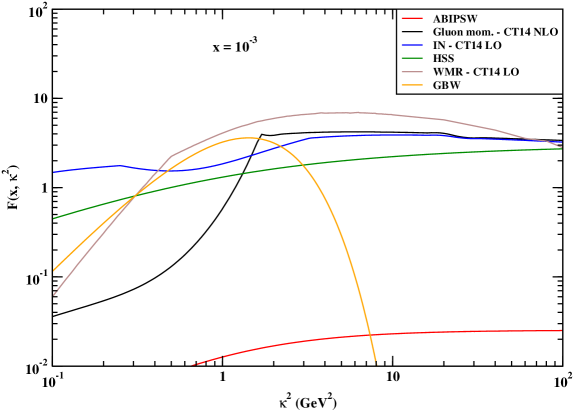
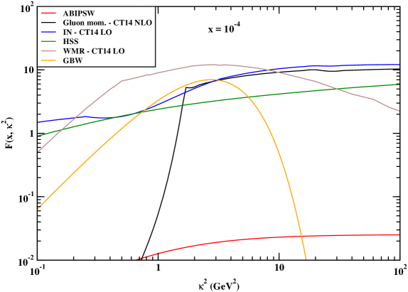
Figure 1: $\kappa^{2}$-dependence of all UGD models for $x=10^{-3}$ and $10^{-4}$.

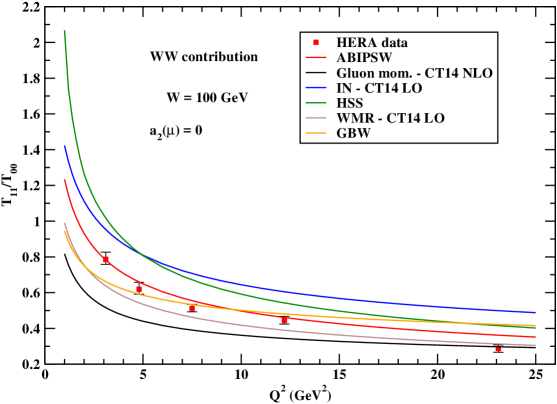
Figure 2: $Q^{2}$-dependence of the helicity-amplitude ratio $T_{11}/T_{00}$ for all the considered UGD models at $W=100$ GeV. In the twist-2 DA we have put $a_{2}(\mu_{0}=1\mbox{ GeV})=0$ and the $T_{11}$ amplitude has been calculated in the WW approximation.

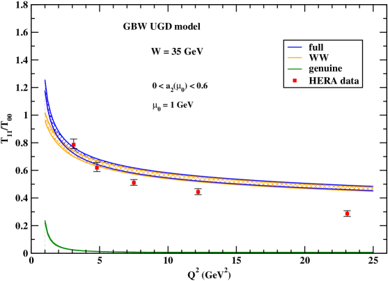
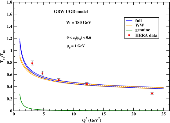
Figure 3: $Q^{2}$-dependence of the helicity-amplitude ratio $T_{11}/T_{00}$ for the GBW UGD model at $W=35$ (top) and 180 GeV (bottom). The full, WW and genuine contributions are shown. The shaded bands give the effect of varying $a_{2}(\mu_{0}=1\mbox{ GeV})$ between 0. and 0.6.

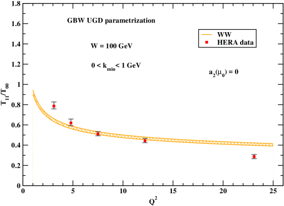
Figure 4: $Q^{2}$-dependence of the helicity-amplitude ratio $T_{11}/T_{00}$ for the GBW UGD model at $W=100$ GeV. The band is the effect of a lower cutoff in the $\kappa$-integration, ranging from 0. to 1 GeV. In the twist-2 DA we have put $a_{2}(\mu_{0}=1\mbox{ GeV})=0$ and the $T_{11}$ amplitude has been calculated in the WW approximation.

III.1 Tools and systematics

All numerical calculations we done in Fortran, making use of specific CERNLIB routines cernlib to perform numerical integrations and the computation of (poly-)gamma functions. In order to deal with all the considered UGD models, we found advantageous to create a modular library which allowed us to bind and call all sets via a unique and simple interface, serving at the same time as a working environment for the creation of new, user-customized UGD parametrizations.

The uncertainty coming from the numerical 2-dimensional over $\kappa$ and $y$ in Eqs. (4), (5) and (7) was directly estimated by the Dadmul integrator cernlib and it was constantly kept below 0.5%. In the case of the HSS and WMR models, one should take into account of an extra-source of systematic uncertainties coming from the integration on $\nu$ (Eq. (16)) and on $z$ and $\kappa_{t}^{2}$ (Eqs. (25) and (26)), respectively. Even in this case, we managed to keep the numerical error very small.

Furthermore, it is worth to note that for all the UGD models involving the use of standard PDF parametrizations, it was needed to put a lower cut-off in $\kappa$, in order to respect the kinematical regime where each set has been extracted. We gauged the effect of using different PDF parametrizations by making tests with the most popular sets extracted from global fits, namely MMHT14 Harland-Lang:2014zoa , CT14 Dulat:2015mca and NNPDF3.0 Ball:2014uwa , as provided by the LHAPDF Interface 6.2.1 Buckley:2014ana , after imposing a provisional cut-off of $\kappa_{\rm min}^{\rm(test)}=1$ GeV. We checked that the discrepancy among the various cases is small or negligible. Then, we did the final calculations by using the CT14 parametrization, which allowed us to integrate over $\kappa$ down to $\kappa_{\rm min}=0.3$ GeV. Results with the gluon momentum derivative and the WMR model were obtained by imposing such a cut-off, while we adopted a dynamic strategy as for the IN one: we cut the contribution coming from the IN hard component (Eq. (14)), at $\kappa_{\rm min}$, while no cut-off was imposed for the soft component (Eq. (13)). With respect to this model, we made further tests by considering the effect of using different DGLAP inputs (see Table I of Ref. Ivanov:2000cm ) for the parameters $Q_{c}$, $\kappa_{h}$ and $\mu_{\rm soft}$ entering Eqs. (13) and (14). No significant discrepancy among them was found, so we gave our results for the IN model by using the so-called CTEQ4L DGLAP input.

Following the definition of IN and WMR models, the PDF set was taken at LO, while the NLO one was employed in the gluon momentum derivative parametrization. Moreover, as for the HSS UGD parametrization, we checked that the discrepancy between the so-called improved setup given in Eq. (19) and the standard one (see, e.g. Ref. Chachamis:2015ona ) is negligible when considering the helicity-amplitude ratio $T_{11}/T_{00}$.

IV Discussion

In this paper we have proposed an observable that is well measured in the experiments at HERA (and could be studied in possible future electron-proton colliders) – the dominant helicity amplitudes ratio for the electroproduction of vector mesons – as a nontrivial testfield to discriminate the models for the unintegrated gluon distribution in the proton.

The main motivation of our study are the features, observed at HERA, of polarization observables for exclusive vector meson electroproduction. In the cases of both longitudinal and transverse polarizations, the measured cross sections demonstrate similar dependencies on kinematic variables: specific $Q^{2}$ scaling, $t$- and $W$-dependencies that are distinct from the ones seen in soft diffractive exclusive processes. This indicates that the dominant physical mechanism in both cases is the scattering of a small transverse-size, $\sim 1/Q$, dipole on a proton.

On the theoretical side we have a description in $\kappa$-factorization, where the nonperturbative physics is encoded in the unintegrated gluon distribution, ${\cal F}(x,\kappa^{2})$, and in the vector meson twist-2 and twist-3 DAs (which includes both WW and genuine twist-3 contributions), that parameterize the probability amplitudes for the transition of 2- and 3- parton small-transverse-size colorless states to the vector meson.

In our analysis we have considered six models for ${\cal F}(x,\kappa^{2})$, which exhibit rather different shape of $\kappa$-dependence in the region, $\kappa^{2}\sim$ few $\rm{GeV}^{2}$, relevant for the kinematic of the $\rho$-meson electroproduction at HERA, as shown in Fig. 1.

In our numerical study we have found rather weak sensitivity of our predictions for the helicity-amplitude ratio to the physics encoded in the meson DAs (though values of longitudinal and transverse amplitudes separately depend strongly on the model for DAs). As an example, in Fig. 3 we have presented results for the GBW model of ${\cal F}(x,\kappa^{2})$. Here the dominance of the WW contribution over the genuine twist-3 one is clearly seen. Besides, we have found rather moderate dependence of our observable on the shape of twist-2 DA. Indeed, varying the value of $a_{2}$ in a wide range in comparison to the value $a_{2}(\mu_{0})=0.18\pm 0.10$ obtained from the QCD sum rules Ball:1998sk , and the one calculated recently on the lattice in Ref. Braun:2016wnx , $a_{2}(\mu=2\mbox{ GeV})=0.132\pm 0.027$, we have found small variation of the amplitude ratio, on the level of the experimental errors.

Another important issue is the small-size color dipole dominance that allows us to use results for the $\gamma^{*}\to\rho$ IF calculated unambiguously in terms of the meson DAs. To clarify this question we have introduced a cut-off in the $\kappa$-integration and studied the stability of our predictions on the excluded region of small gluon transverse momenta. In Fig. 4, considering again GBW model as an example, we have shown that the sensitivity of our predictions to the region of small $\kappa$ is indeed not strong, the variation of our results is lower than or comparable to the data errors.

In this way we have seen that the dominance of the small-size dipole production mechanism is supported both by the qualitative features of the data and by the theoretical calculations in $\kappa$-factorization. This gives evidence to our main statement that, having precise HERA data on the helicity-amplitude ratio, one can obtain important information about the $\kappa$-shape of the UGD. To demonstrate this in Fig. 2 we have confronted HERA data with the predictions calculated with six different UGD models. We have seen that none of the models is able to reproduce data over the entire $Q^{2}$ range and that HERA data on the transverse to longitudinal amplitudes ratio are really precise enough to discriminate predictions of different UGD models.

Our work is closely related to the study of Ref. Besse:2013muy , where the same process was investigated in much detail in the dipole approach. In this case the process helicity amplitudes are factorized in terms of the dipole cross section $\hat{\sigma}(x,r)$. The $\kappa$-factorization and the dipole approach are mathematically related through a Fourier transformation, but the latter approach represents the most natural language to discuss saturation effects, due to a distinct picture of saturation for the $\hat{\sigma}(x,r)$ dependence on $r$ for the dipole sizes that exceed the reverse saturation scale, $r\geq 1/Q_{S}(x)$. Besides, nonlinear evolution equations that determine the $x$-dependence of $\hat{\sigma}(x,r)$ and include saturation effects are formulated in the transverse coordinate space.

In Ref. Besse:2013muy several models for $\hat{\sigma}(x,r)$ (including the GBW model adopted by us here) that include saturation effects, and whose parameters were fitted to describe inclusive DIS data, were considered. They were used to make predictions for vector meson exclusive production at HERA kinematics. It was found in Ref. Besse:2013muy that the predictions of GBW and of other more elaborated dipole models are close to each other and give rather good, but not excellent, description of HERA data at virtualities bigger than $Q^{2}\approx 5\,\rm{GeV}^{2}$.

Another interesting issue studied in Ref. Besse:2013muy is the radial distribution of the dipoles, that contributes to the longitudinal and the transverse helicity amplitudes for $\rho$-production. It was shown that for large $Q^{2}$ both helicity amplitudes are dominated by the contributions of small size dipoles, which is another source of evidence in favour of the small-size dipole mechanism for the hard vector meson electroproduction at HERA. Besides, as it is shown in Ref. Besse:2013muy , in the case of large $Q^{2}$, see the right panels of Fig. 17 in Ref. Besse:2013muy for $Q^{2}=10\,\rm{GeV}^{2}$, the relevant values of $r$ are considerably lower than those where the dipole cross section $\hat{\sigma}(x,r)$ starts to saturate. This is perhaps not surprising, since the estimated value of the saturation scale at HERA energies is not big, $Q^{2}_{S}\sim 1\,\rm{GeV}^{2}$. Therefore one can anticipate that saturation effects for hard vector meson electroproduction at HERA do not play a crucial role. The region of large values of $r$, where the dipole cross section saturates, represents only a corner of $r$-integration region for both helicity amplitudes in the dipole approach. In the language of $\kappa$-factorization, that we use in this work, the saturation region is related to the $\kappa$-integration region of small $\kappa$. Our calculations for the GBW model with $\kappa$ cutoff, see Fig. 4, show that, indeed, the helicity-amplitude ratio for hard meson electroproduction at HERA is not very sensitive to this saturation region. Therefore we believe that HERA data allow to obtain nontrivial information on the UGD shape (or equivalently, about the $r$ shape of the dipole cross section) in the kinematic range where the linear evolution regime is still dominant.

Finally, as our closing statement, we recommend that further tests of models for the unintegrated gluon distribution, as well as possible new model proposals, take into due account our suggestion to utilize the important information encoded in the HERA data on the helicity structure in the light vector meson electroproduction.

V Acknowledgments

We thank M. Hentschinski for fruitful discussions.
FGC acknowledges support from the Italian Foundation “Angelo della Riccia”. AP acknowledges support from the INFN/QFT@colliders project.

References

- (1) V.N. Gribov, L.N. Lipatov, Sov. J. Nucl. Phys. 15 (1972) 438; G. Altarelli, G. Parisi, Nucl. Phys. B 126 (1977) 298; Y.L. Dokshitzer, Sov. Phys. JETP 46 (1977) 641.
- (2) J.C. Collins, L. Frankfurt and M. Strikman, Phys. Rev. D 56 (1997) 2982 [hep-ph/9611433].
- (3) A.V. Radyushkin, Phys. Rev. D 56 (1997) 5524 [hep-ph/9704207].
- (4) V.S. Fadin, E.A. Kuraev, L.N. Lipatov, Phys. Lett. B60 (1975) 50; E.A. Kuraev, L.N. Lipatov and V.S. Fadin, Zh. Eksp. Teor. Fiz. 71 (1976) 840 [Sov. Phys. JETP 44 (1976) 443]; 72 (1977) 377 [45 (1977) 199]; Ya.Ya. Balitskii and L.N. Lipatov, Sov. J. Nucl. Phys. 28 (1978) 822.
- (5) J.R. Andersen et al. [Small x Collaboration], Eur. Phys. J. C 48 (2006) 53 [hep-ph/0604189]; Eur. Phys. J. C 35 (2004) 67 [hep-ph/0312333]; B. Andersson et al. [Small x Collaboration], Eur. Phys. J. C 25 (2002) 77 [hep-ph/0204115].
- (6) R. Angeles-Martinez et al., Acta Phys. Polon. B 46 (2015) no.12, 2501 [arXiv:1507.05267 [hep-ph]].
- (7) F.D. Aaron et al. [H1 Collaboration], JHEP 1005 (2010) 032 [arXiv:0910.5831 [hep-ex]].
- (8) S. Chekanov et al. [ZEUS Collaboration], PMC Phys. A 1 (2007) 6 [arXiv:0708.1478 [hep-ex]].
- (9) I.V. Anikin, D.Yu. Ivanov, B. Pire, L. Szymanowski and S. Wallon, Nucl. Phys. B 828 (2010) 1 [arXiv:0909.4090 [hep-ph]].
- (10) I.V. Anikin, A. Besse, D.Yu. Ivanov, B. Pire, L. Szymanowski and S. Wallon, Phys. Rev. D 84 (2011) 054004 [arXiv:1105.1761 [hep-ph]].
- (11) A. Besse, L. Szymanowski and S. Wallon, Nucl. Phys. B 867 (2013) 19 [arXiv:1204.2281 [hep-ph]].
- (12) A. Besse, L. Szymanowski and S. Wallon, JHEP 1311 (2013) 062 [arXiv:1302.1766 [hep-ph]].
- (13) D.Yu. Ivanov, R. Kirschner, Phys. Rev. D 58 (1998) 114026 [hep-ph/9807324].
- (14) P. Ball, V.M. Braun, Y. Koike and K. Tanaka, Nucl. Phys. B 529 (1998) 323 [hep-ph/9802299].
- (15) S. Dulat et al. Phys. Rev. D 93 (2016) no.3, 033006 [arXiv:1506.07443 [hep-ph]].
- (16) I.P. Ivanov, N.N. Nikolaev, Phys. Rev. D 65 (2002) 054004 [hep-ph/0004206].
- (17) N.N. Nikolaev, B.G. Zakharov, Phys. Lett. B 332 (1994) 177 [hep-ph/9403281]; Z. Phys. C 53 (1992) 331.
- (18) M. Hentschinski, A. Sabio Vera, C. Salas, Phys. Rev. Lett. 110 (2013) no.4, 041601 [arXiv:1209.1353 [hep-ph]].
- (19) G. Chachamis, M. Deák, M. Hentschinski, G. Rodrigo, A. Sabio Vera, JHEP 1509 (2015) 123 [arXiv:1507.05778 [hep-ph]].
- (20) I. Bautista, A. Fernandez Tellez, M. Hentschinski, Phys. Rev. D 94 (2016) no.5, 054002 [arXiv:1607.05203 [hep-ph]].
- (21) K.J. Golec-Biernat, M. Wüsthoff, Phys. Rev. D 59 (1998) 014017 [hep-ph/9807513].
- (22) G. Watt, A.D. Martin, M.G. Ryskin, Eur. Phys. J. C 31 (2003) 73 [hep-ph/0306169].
- (23) CERNLIB Homepage: http://cernlib.web.cern.ch/cernlib.
- (24) L.A. Harland-Lang, A.D. Martin, P. Motylinski, R.S. Thorne, Eur. Phys. J. C 75 (2015) no.5, 204 [arXiv:1412.3989 [hep-ph]].
- (25) R.D. Ball et al. [NNPDF Collaboration], JHEP 1504 (2015) 040 [arXiv:1410.8849 [hep-ph]].
- (26) A. Buckley, J. Ferrando, S. Lloyd, K. Nordström, B. Page, M. Rüfenacht, M. Schnherr, G. Watt, Eur. Phys. J. C 75 (2015) 132 [arXiv:1412.7420 [hep-ph]].
- (27) V.M. Braun et al., JHEP 1704 (2017) 082 [arXiv:1612.02955 [hep-lat]].