Application of End-to-End Deep Learning in Wireless Communications Systems

Abstract

Deep learning is a potential paradigm changer for the design of wireless communications systems (WCS), from conventional handcrafted schemes based on sophisticated mathematical models with assumptions to autonomous schemes based on the end-to-end deep learning using a large number of data. In this article, we present a basic concept of the deep learning and its application to WCS by investigating the resource allocation (RA) scheme based on a deep neural network (DNN) where multiple goals with various constraints can be satisfied through the end-to-end deep learning. Especially, the optimality and feasibility of the DNN based RA are verified through simulation. Then, we discuss the technical challenges regarding the application of deep learning in WCS.

I Introduction

The deep learning, which is based on the deep neural network (DNN) that emulates the neurons of the brain, has gained in great popularity in recent days. The current enthusiasm for deep learning is mainly due to its significant performance gains over conventional schemes[1, 2, 3]. For example, the deep learning based image classification schemes can achieve far more accurate performance than handcrafted conventional schemes based on the analytic models, and they have even surpassed the human-level performance. The application of deep learning is not confined to the simple classification task but it also shows notable performance in more complicated tasks, such as the semantic scene understanding [2].

The advent of deep learning can change the research paradigm from designing scheme through careful engineering based on mathematical models to end-to-end learning based scheme in which the proper scheme is autonomously designed by observing a large amount of data, cf. Fig. 1. For example, conventional image classification schemes rely on the handcrafted complex feature detectors which are engineered by the expertise, e.g., edge detector. However, in case of deep learning based image classification, feature detectors that are far more accurate than conventional detectors can be derived by a DNN structure from a large number of image data. Accordingly, in the era of deep learning, 1) the preparation, selection and pre-processing of data to be used in DNN structure, 2) the determination of proper DNN structure and 3) the interpretation of the output of DNN, become more important than the development of analytic schemes from the mathematical system model which usually contains assumption to make analysis feasible.

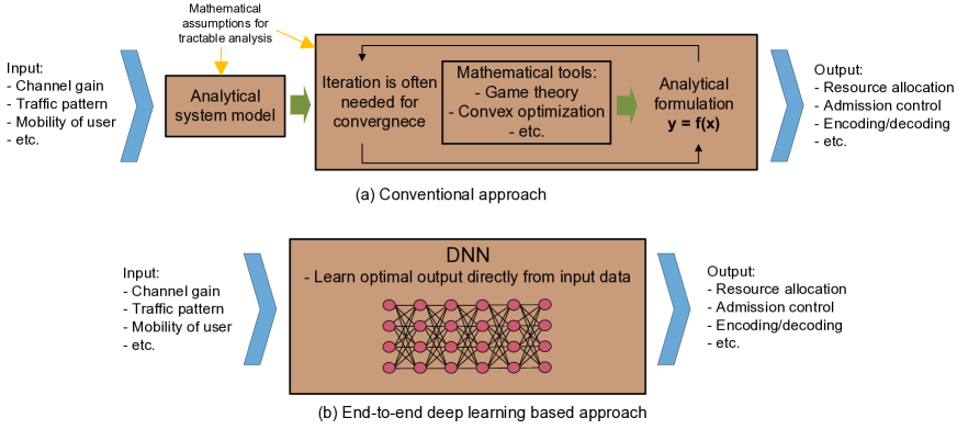
Figure 1: Comparison of end-to-end deep learning based approach with conventional approach.

In recent days, the deep learning has begun to be applied to the many research areas of wireless communications systems (WCS), especially in the classification tasks such as traffic and channel estimation. The authors of [4] showed that the type of data traffic can be determined accurately with DNN. Moreover, in [5], the channel estimation and signal detection in orthogonal frequency-division multiplexing (OFDM) systems was considered based on the deep learning. Furthermore, the deep learning is also applied to more complicated tasks than just classification, e.g., the encoder and decoder for sparse code multiple access (SCMA), were developed using a DNN based autoencoder in [6].

One interesting characteristic of deep learning is that the DNN can be considered as a universal approximator [7] which is capable of approximating an arbitrary function such that it can emulate the behavior of highly nonlinear and complicated systems. Moreover, given that the DNN can be trained in an end-to-end manner which treats the operation as a black box, i.e., end-to-end deep learning, the use of DNN enables the exploit of the optimal strategy without solving the complicated problems explicitly, cf. Fig. 1. In this sense, the deep learning has been applied for the resource allocation (RA) of WCS where the exploitation of optimization problems was taken into account previously. Unlike conventional approaches which derive the optimal strategy for RA from the analytic system model with assumptions, the deep learning based approach can derive the optimal strategy directly from actual channel data such that it can adapt to the environment and the performance is likely to be higher in practice. Moreover in the deep learning based approach, the general solver for the optimization problem of RA can be derived such that the optimal strategy can be found with low computation time even when the parameters, e.g., channel gain, change [5, 8]. The authors of [7] used a DNN to regenerate the transmit power of weighted minimum mean square error (WMMSE)-based scheme in order to resolve the problem of high computation time of the WMMSE-based scheme. Moreover, in [8], the transmit power was optimized to maximize either spectral efficiency (SE) or energy efficiency (EE) where the optimal strategy for transmit power control is learned through an end-to-end deep learning without needing to derive explicit mathematical formulation.

In this article, we focus on the application of deep learning in the WCS. To this end, we first address basic principles of deep learning. Then, we investigate the DNN architecture which can be trained to derive general strategy for RA that can achieve diverse goals, i.e., maximization of SE, EE, and minimization of transmit power, while satisfying constraints on interference and quality-of-service (QoS). Finally, the research challenges regarding the application of deep learning will be addressed before concluding the article.

II Fundamentals of Deep Learning

In this section, we first describe the basic component and structure of Neural network (NN) and how to train it. Then, we turn our attention to deep learning and its application to WCS.

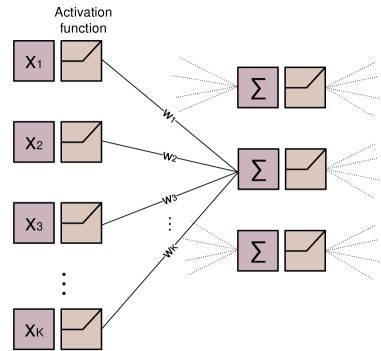
Figure 2: Basic structure of NN.

II-A Structure of Neural Network

NN which comprises DNN, is a subcategory of machine learning which mimics the operation of brain. Through the extensive experiment, it was found that the brain is composed of neurons which are connected to each other. The neuron takes the outputs of other neurons as its input and activates its output when the inputs satisfy a certain condition, i.e., it can be considered as a biological switch. In the NN, the connection between neurons (nodes) is modeled by the matrix multiplication and the activation of neurons is modeled by the functions which look similar to a step function, e.g., sigmoid and rectified linear unit (ReLU), which provide the ability to model non-linear characteristic to the NN. The basic structure of NN is shown in Fig.2. Accordingly, the NN can be considered as the collection of matrix computation and activation functions and the calculation of output of NN for one sample data, i.e., inference, usually requires low computational overhead.

According to the existence of feedback loop in the network, the NN can be divided into two categories.

• Feedforward neural network (FNN): In FNN, there is no feedback loop such that the previous input data would not affect the current output, i.e., memoryless. The FNN is used when the data is not correlated to each other, e.g., image data. In WCS, this type of NN is used for the spectrum sensing and power control of users [7, 8, 9].

• Recurrent neural network (RNN): The connection of nodes in RNN forms a cycle such that the current input can affect the output of the next input, i.e., the DNN has memory. Accordingly, this type of NN is used for the data which has a temporal correlation. The data with temporal correlation in WCS, e.g., channel estimation, has been dealt with the RNN [4].

II-B Overview on Training of Neural Network

The training of NN, i.e., determination of weights and biases of NN, is not obvious. In fact, the lack of appropriate way to find weights and biases has brought the first depression of research on NN after its first development in 1950s. In 1980s, an efficient way to train NN, i.e., back-propagation algorithm, has been developed [10] which leads the second booming of the research on NN. The back-propagation algorithm is based on the gradient descent technique such that the error of the NN, e.g., difference between the target and the output, is propagated in backward direction to update weights and biases according to the gradient, e.g., strengthen the parameters when the output is correct and weakening the parameters when the output is incorrect. By using the back-propagation algorithm, the NN can be trained efficiently.

According to the training methodology, the NN can be divided into three categories, same as general machine learning algorithms.

• Supervised learning: In the supervised learning, the training data is labeled such that the NN can compare its output with the ground truth. This type of learning is widely used in the classification, e.g., the detection of primary user in cognitive radio (CR) systems [9].

• Unsupervised learning: In the unsupervised learning, the data is not labeled such that the NN should autonomously derive the meaningful features from the input samples, e.g., clustering. In [11], the encoder and decoder for SCMA system has been found using the autoencoder structure in unsupervised learning.

• Reinforcement learning: In the reinforcement learning, the learning of NN is conducted by trial-and-error. Especially, for a given input data, the proper action can be found through NN and reward can be observed for the selected action. Then, the NN is trained to provide better action which gives higher reward. Anti-jamming strategy for secondary users in CR systems was developed based on deep reinforcement learning in [12].

II-C Deep Neural Network

With the back-propagation algorithm, the NN can be trained efficiently. Nonetheless, it was observed that the NN with a large number of layers which is essential to achieve human-like functionality, is hard to be trained, mainly due to the vanishing gradient problem, and the lack of proper input data and computation power, and it results in the second depression of research on NN for about 20 years.

Recently, the use of NN with a large number of layers, which is known as DNN, becomes possible, mainly due to the following four reasons [3].

• Availability of large dataset: Due to the development of sensors and Internet, the collection of a large number of data is enabled which is essential for the DNN to learn general features. For instance, the development of ImageNet, which is a database of image that contains more than 15,000,000 labeled images, becomes the basis for the big success of DNN in the image classification.

• Use of better activation function: The problem of vanishing gradient is mainly caused by the use of inefficient activation functions whose gradient is smaller than 1, e.g., sigmoid. However, in the DNN, the activation function with better gradient characteristics, e.g., ReLU, is used such that the error at the output can be properly propagated through the layers.

• Higher computation power: Although the inference of output for one input data requires small computational overhead, the training can take a long computation time due to the large number of training data. However, thanks to the development of parallel computation based on graphics processing unit, this training procedure can be conducted with low computation time.

• Efficient initialization methodology: In the DNN, the initialization technique is utmost important to achieve high performance without falling into poor local minimum. Recently, good initialization techniques such as Restricted Boltzmann Machine (RBM) and Xavier initialization enable the efficient training of DNN [13].

II-D Application of Deep Neural Network in Wireless Communications Systems

The DNN is well suited for WCS because the WSC usually deals with a large amount of data and has complex system model which is hard to analyze at hand, and its potential application in WCS is enormous. Especially, unlike conventional approach in WCS where the specific channel model is assumed such that its performance cannot be guaranteed when the assumed channel is different from the actual channel, the DNN based approach is able to adapt its operation according to the environment without relying on the specific channel model. Moreover, same as image classification, the DNN based approach might provide better schemes than conventional handcrafted schemes, especially, when the problem is complex and hard to analyze by empirical formulation [6, 9, 8].

III Resource Allocation based on End-to-End Deep Learning

In this section, we investigate the DNN based RA. To this end, we first describe the considered system model which comprises underlay device-to-device (D2D) communication. Then, the proposed DNN model for RA whose objective is either maximizing SE, EE or minimizing total transmit power, is addressed and the optimality of the DNN based RA is examined through simulation.

III-A System Model and Resource Allocation

We consider an RA for the multi-channel cellular system with underlay D2D communication where the data transmission of $N$ D2D user equipments (DUEs) takes place simultaneously with cellular transmission, and users are randomly distributed over an area $D\times D$. The channel gain between $i$-th transmitter and $j$-th receiver for channel $m$ is denoted as $h^{m}_{i,j}$, where the index $0$ is assigned to the cellular user equipment (CUE) and base station (BS). The considered system model is depicted in Fig. 3.

In the considered RA, the transmit power of DUEs allocated to each channel, which we denote as $P^{m}_{i}$ where $m$ and $i$ are the index of channel and DUE, respectively, has to be determined to either 1) maximize SE, 2) maximize EE, or 3) minimize total transmit power. In the RA, we take into account three constraints. First, the transmit power allocated to each channel should be non-negative and the sum of transmit power for a single DUE should not exceed the maximum transmit power, $P_{\textrm{T}}$ (i.e., transmit power constraint). Second, the amount of interference caused to cellular transmission must be less than the threshold $I_{\textrm{T}}$ (i.e., interference constraint). Third, each D2D transmission should satisfy the minimum QoS requirement, i.e., the SE achieved by each DUE has to be larger than the threshold, $R_{\textrm{T}}$ (i.e., QoS constraint).

Given that the considered RA can be formulated into a non-convex problem, it is hard to derive the optimal RA analytically, therefore, iterative methods based on Lagrangian relaxation have been considered previsouly [14]. However, this approach requires a number of iterative computations, which possibly increases the computation time [7, 8], such that the real time operation can be hindered. However, in the DNN based RA, the generic solver is derived autonomously through DNN which involves only simple matrix operations, so that the proper RA for any channel condition can be found with a low computational complexity without iteration.

III-B Resource Allocation based on Deep Neural Network

In our DNN model, the total transmit power of each DUE and the proportion of transmit power allocated to each channel by individual DUE are found jointly using separate DNN module, which are the total transmit power network (Tnet) and the power allocation network (Pnet), cf. Fig. 3. The channel gain is pre-processed for better training performance such that it is converted to dB and normalized to have zero mean and unit variance, and these pre-processed channel gain becomes the input of two networks, Tnet and Pnet.

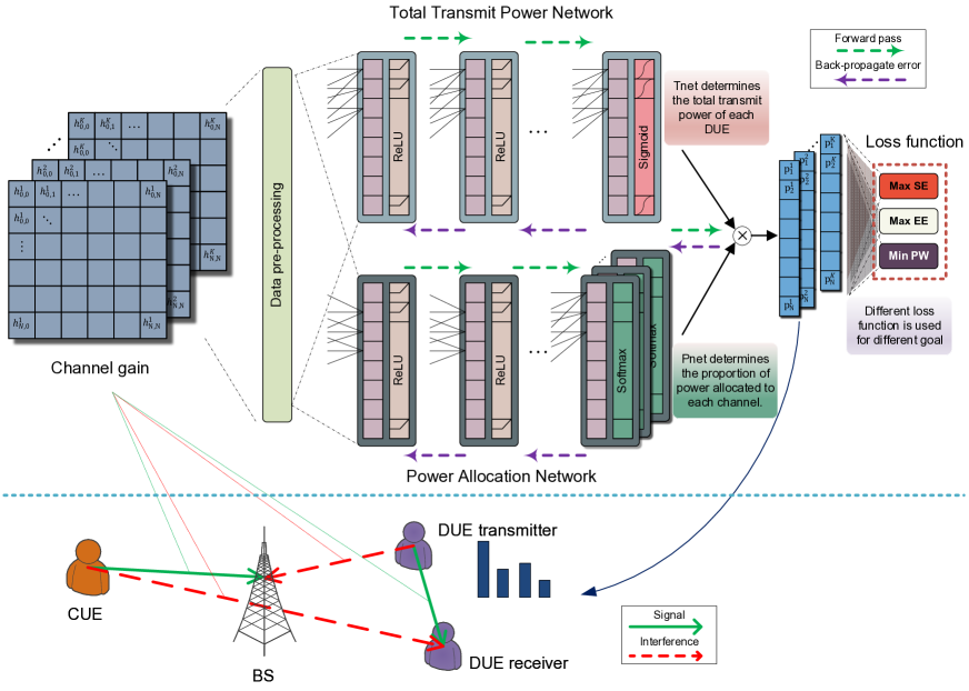
Figure 3: Considered system model and DNN structure for the RA.

The Tnet and Pnet are composed of sub-modules which comprised a FC layer and ReLU which is used as an activation function. Given that the each output of the Tnet should be less than the maximum transmit power, $P_{\textrm{T}}$, we have implemented the sigmoid which is multiplied by the $P_{\textrm{T}}$ at the end of the Tnet, where the output of sigmoid is between 0 and 1. On the other hand, the proportion of transmit power allocated to each channel for each DUE is determined by the Pnet, such that we consider $N$ softmax modules as the last layer of Pnet where each softmax module has $M$ outputs. Given that the sum of a single softmax module is 1, it is appropriate to model the proportion of transmit power allocated to channels for individual DUE. Finally, by multiplying the outputs of both Tnet and Pnet, the transmit power of DUEs allocated to each channel can be found. It should be noted that the same DNN structure with different values of weights and biases can be used for three different objectives such that it is efficient in practice in terms of reusing the same DNN structure.

In order to find the optimal set of weights and biases, our proposed DNN model has to be trained first. To this end, the channel samples for training must first be collected by either measurement or simulations using well-known channel model. Hybrid use of measurement data and synthetic data, where the DNN is initially trained with synthetic channel data, and then, trained with a few actually measured data for fine tuning, which is known as a transfer learning, is also possible.

After the channel samples are prepared, the proposed DNN can be trained through a back-propagation algorithm. For the training, in order to achieve goal while satisfying constraints, the weighted sum of objective function and the functions on constraints is taken into account. Accordingly, in order to train DNN model to maximize the SE, the loss function, $L_{\textrm{SE}}$, can be set as $L_{\textrm{SE}}=-\sum\textrm{SE}_{i}+\lambda_{1}\sum\tanh\left([I^{k}_{\textrm{CUE}}-I_{\textrm{T}}]^{+}\right)+\lambda_{2}\sum\tanh\left([\textrm{SE}_{i}-R_{\textrm{T}}]^{+}\right)$, where $\lambda_{1}$, $\lambda_{2}$ are the controlling parameters, $\textrm{SE}_{i}$ is the SE of DUE $i$, and $I^{k}_{\textrm{CUE}}$ is the interference caused to CUE at channel $k$.

As can be seen from the formulation, the loss function increases as the SE of DUEs decreases and at the same time when the interference and QoS constraints are not satisfied. Given that the DNN is trained to reduce the loss, through training, the SE of DUEs will be increased and the violation of interference and QoS constraint will be reduced. Note that $\lambda_{1}$ and $\lambda_{2}$ determine the penalty for the violation of constraints.

Similarly, the loss functions to maximize EE, which we denote as $L_{\textrm{EE}}$ can be written as $L_{\textrm{EE}}=-\sum\textrm{EE}_{i}+\lambda_{1}\sum\tanh\left([I^{k}_{\textrm{CUE}}-I_{\textrm{T}}]^{+}\right)+\lambda_{2}\sum\tanh\left([\textrm{SE}_{i}-R_{\textrm{T}}]^{+}\right)$ and the loss function to minimize the total transmit power, which we denote as $L_{\textrm{TP}}$, can be written as $L_{\textrm{TP}}=\sum P^{m}_{i}+\lambda_{1}\sum\tanh\left([I^{k}_{\textrm{CUE}}-I_{\textrm{T}}]^{+}\right)+\lambda_{2}\sum\tanh\left([\textrm{SE}_{i}-R_{\textrm{T}}]^{+}\right)$. Although the considered loss functions are different from loss functions which are commonly considered in the deep learning researches, e.g., cross entropy, the back-propagation based learning is still possible because all the loss functions are differentiable.

After the proper loss function is determined, the training of DNN can be conducted efficiently using off-the-shelf stochastic gradient descent algorithms, e.g., Adaptive Moment Estimation algorithm. After training, the appropriate transmit power allocated to each channel can be determined by feeding the current channel gain to the trained DNN.

III-C Performance Evaluation

We compare the performance of the proposed DNN based RA with the optimal performance which is found through an exhaustive search. For the performance evaluation, we assume that the number of DUE transmission pairs and the number of channels is two such that the finding optimal performance through exhaustive search is computationally plausible. The maximum transmit power and the circuit power are set to 23 dBm, the bandwidth is set to 10 MHz, the noise density is set to -173dBm/Hz, $I_{\textrm{T}}$ = -55 dBm and $R_{\textrm{T}}$ = 3 bps/Hz. Moreover, the simplified path loss model with path loss coefficient $10^{3.453}$ and path loss exponent $3.8$ is considered and an independent and identically distributed (i.i.d.) circularly symmetric complex Gaussian (CSCG) random variable with a mean of zero and a variance of one is used for multipath fading.

For the DNN model, we assume that the number of layers for Tnet and Pnet is 4 and the number of hidden nodes for FC layer is 100. Moreover, 40,000 channel samples are used for the training and the learning rate are adaptively changed over training epoch. In the performance evaluation, we examine the average SE, the average EE, and the total transmit power of each DUE of the DNN based RA whose objectives are the maximization of SE (Max. SE), the maximization of EE (Max. EE) and the minimization of total transmit power (Min. PW). Moreover, the optimal performance of RA for considered goals is also examined. Although we do not show graphically, the computation time of the DNN based RA was measured at 1.1 milliseconds while the time required to find the optimal solution is measured at 2743 milliseconds which reveals the benefit of the DNN based RA.

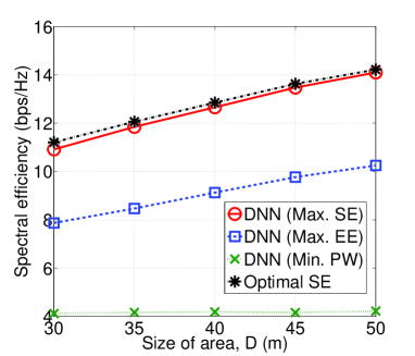
Figure 4: Spectral efficiency vs. size of area.

Figure 5: Energy efficiency vs. size of area.

Figure 6: Total transmit power vs. size of area.

In Figs. 4, 5, and 6, we show the average SE, the average EE, and the total transmit power of DUE, respectively, as a function of the size of area, $D$. As can be seen from the simulation results, the DNN based RA achieves the close-to-optimal performance. For example, the SE of DNN based RA for the SE maximization achieves 97% of the optimal SE. The outage probability that interference or QoS constraint is violated is measured to be less than 2.1% which is sufficiently low. Moreover, even when the constraint is violated, the level of violation is minor. These simulation results affirm the applicability and benefits of the DNN based RA because the DNN based RA has much lower computation time compared with the optimal scheme.

IV Research Challenges

In the following, we discuss some research challenges for future usage of deep learning in WCS.

IV-A Measured Channel Data as Training Sample

In the deep learning based approach, the DNN autonomously finds the optimal strategy or meaningful features directly from data instead of using handcrafted mathematical system model. Accordingly, in order to achieve high performance in deep learning, a large number of training samples regarding WCS, e.g., channel gain data, for different scenarios has to be collected through actual measurement. The problem regarding the preparation of training data could be solved by using the DNN based on a generative model, e.g., generative adversarial network (GAN), which shows big success in the image synthesis, to generate realistic synthetic training data.

IV-B Distributed Operation and Inaccurate Channel Information

Unlike image classification in which all input data can be easily obtained by the single node, in WCS, the input data of the DNN, e.g., channel gain, is hard to be obtained by the single node which executes the DNN functionality due to high signaling overhead, especially when the number of users is large. Moreover, the input data of DNN for practical WCS is likely to contain error due to the inaccurate measurement and delayed channel feedback. To solve the problem of distributed operation, the distributed deep learning can be considered [15] and to solve the problem of inaccurate channel information, denoising autoencoder can be taken into account.

IV-C Computation Complexity

The control of WCS, e.g., RA, has to be conducted within a very short time period, i.e., several milliseconds, due to the short frame length. Moreover, the deep learning based scheme for WCS should have low computational complexity because it could be operated on the mobile device which has limited computation power. Although we show that the DNN based RA has a very low computation time compared with the optimal scheme, storing the trained DNN model can become overhead to the mobile device. Moreover, online learning in which each mobile device trains its own model based on the collected channel samples, can be taken into account in order to further improve the performance, and in this case, the overhead of DNN based schemes can be large. This problem can be solved by using newly developed AI accelerator chip, e.g., tensor processing unit (TPU) by Google, which is likely to be implemented in mobile device because more technologies based on deep learning are now applied to mobile devices.

V Conclusions

In this article, the application of DNN for WCS through autonomous end-to-end deep learning as opposed to conventional handcrafted engineering based on the mathematical modeling, has been discussed. In particular, the deep learning based RA has been addressed whose optimal strategy is hard to be obtained in conventional approach. It has been confirmed by performance evaluation that the DNN based RA can achieve close-to-optimal performance with low computation time for various objectives of RA reusing the same DNN structure. We have also outlined the challenges regarding the application of deep learning in the research of WCS.

References

- [1] T. J. O’Shea, J. Corgan, and T. C. Clancy, “Convolutional radio modulation recognition networks,” in Proc. of EANN, Aberdeen, U.K., Sep. 2016.
- [2] A. Karpathy and L. Fei-Fei, “Deep visual-semantic alignments for generating image descriptions,” in Proc. of IEEE CVPR, Boston, MA, USA, Jun. 2015.
- [3] Y. LeCun, Y. Bengio, and G. Hinton, “Deep learning,” Nature, vol. 521, no. 7553, pp. 436–444, May 2015.
- [4] T. J. O’Shea, S. Hitefield, and J. Corgan, “End-to-end radio traffic sequence recognition with deep recurrent neural networks,” arXiv preprint arXiv:1610.00564, 2016.
- [5] H. Ye, G. Y. Li, and B. H. Juang, “Power of deep learning for channel estimation and signal detection in OFDM systems,” IEEE Wireless Commun. Lett., vol. 7, no. 1, pp. 114–117, Feb. 2018.
- [6] M. Kim, N. I. Kim, W. Lee, and D. H. Cho, “Deep learning aided SCMA,” IEEE Commun. Lett., vol. 22, no. 4, pp. 720–723, Apr. 2018.
- [7] H. Sun, X. Chen, Q. Shi, M. Hong, X. Fu, and N. D. Sidiropoulos, “Learning to optimize: Training deep neural networks for wireless resource management,” arXiv preprint arXiv:1705.09412, 2017.
- [8] W. Lee, M. Kim, and D. H. Cho, “Deep power control: Transmit power control scheme based on convolutional neural network,” IEEE Commun. Lett., vol. 22, no. 6, pp. 1276–1279, 2018.
- [9] W. Lee, M. Kim, and D.-H. Cho, “Deep sensing: Cooperative spectrum sensing based on convolutional neural networks,” arXiv preprint arXiv:1705.08164, 2017.
- [10] D. E. Rumelhart and J. L. McClelland, Learning Internal Representations by Error Propagation. MIT Press, 1987, pp. 318–362.
- [11] M. Kim, N. I. Kim, W. Lee, and D. H. Cho, “Deep learning aided SCMA,” IEEE Commun. Lett., vol. 22, no. 4, pp. 720–723, Apr. 2018.
- [12] G. Han, L. Xiao, and H. V. Poor, “Two-dimensional anti-jamming communication based on deep reinforcement learning,” in Proc. of IEEE ICASSP, New Orleans, LA, USA, Mar. 2017.
- [13] X. Glorot and Y. Bengio, “Understanding the difficulty of training deep feedforward neural networks,” in Proc. of AISTATS, Sardinia, Italy, May 2010.
- [14] Y. Jiang, Q. Liu, F. Zheng, X. Gao, and X. You, “Energy-efficient joint resource allocation and power control for D2D communications,” IEEE Trans. Veh. Technol., vol. 65, no. 8, pp. 6119–6127, Aug. 2016.
- [15] P. de Kerret and D. Gesbert, “Robust decentralized joint precoding using team deep neural network,” in Proc. of ISWCS, Lisbon, Portugal, Aug. 2018.