Phase Transition in Matched Formulas and a Heuristic for Biclique Satisfiability

Abstract

A matched formula is a CNF formula whose incidence graph admits a matching which matches a distinct variable to every clause. We study phase transition in a context of matched formulas and their generalization of biclique satisfiable formulas. We have performed experiments to find a phase transition of property “being matched” with respect to the ratio $m/n$ where $m$ is the number of clauses and $n$ is the number of variables of the input formula $\varphi$. We compare the results of experiments to a theoretical lower bound which was shown by Franco and Gelder (2003). Any matched formula is satisfiable, moreover, it remains satisfiable even if we change polarities of any literal occurrences. Szeider (2005) generalized matched formulas into two classes having the same property — var-satisfiable and biclique satisfiable formulas. A formula is biclique satisfiable if its incidence graph admits covering by pairwise disjoint bounded bicliques. Recognizing if a formula is biclique satisfiable is NP-complete. In this paper we describe a heuristic algorithm for recognizing whether a formula is biclique satisfiable and we evaluate it by experiments on random formulas. We also describe an encoding of the problem of checking whether a formula is biclique satisfiable into SAT and we use it to evaluate the performance of our heuristic.

1 Introduction

In this paper we are interested in the problem of satisfiability (SAT) which is central to many areas of theoretical computer science. In this problem we are given a formula $\varphi$ in propositional logic and we ask if this formula is satisfiable, i.e. if there is an assignment of values to variables which satisfies $\varphi$. This is one of the best known NP-complete problems [7]. In this paper we study special classes of formulas whose definition is based on the notion of incidence graph.

Given a formula $\varphi$ in conjunctive normal form (CNF) we consider its incidence graph $I(\varphi)$ defined as follows. $I(\varphi)$ is a bipartite graph with one part consisting of the variables of $\varphi$ and the other part consisting of the clauses of $\varphi$. An edge $\{x,C\}$ for a variable $x$ and a clause $C$ is in $I(\varphi)$ if $x$ or $\overline{x}$ appear in $C$. It was observed by the authors of [2] and [17] that if $I(\varphi)$ admits a matching of size $m$ (where $m$ is the number of clauses in $\varphi$), then $\varphi$ is satisfiable. Later the formulas satisfying this condition were called matched formulas in [10]. Since a matching of maximum size in a bipartite graph can be found in polynomial time (see e.g. [13, 14]), one can check efficiently whether a given formula is matched.

It is clear that if $\varphi$ is a formula on $n$ variables and $m$ clauses then $\varphi$ can be matched only if $m\leq n$. The authors of [10] asked an interesting question: What is the probability that a formula $\varphi$ is matched depending on the ratio $\frac{m}{n}$? We can moreover ask if the property “being matched” exhibits a phase transition.

A phase transition was studied in context of satisfiability [5, 11, 15, 8, 6]. The so-called satisfiability threshold for a given $k$ is a value $r_{k}$ satisfying the following property: A random formula $\varphi$ in $k$-CNF on $n$ variables and $m$ clauses is almost surely satisfiable if $\frac{m}{n}<r_{k}$ and it is almost surely unsatisfiable if $\frac{m}{n}>r_{k}$. For instance the value $r_{3}$ is approximately $4.3$ [8, 6].

In the same sense we can study threshold for property “being matched”. It was shown in [10] that a $3$-CNF $\varphi$ on $n$ variables and $m$ clauses is almost surely matched if $\frac{m}{n}<0.64$. This is merely a theoretical lower bound, and in this paper we perform experimental check of this value. It turns out that the experimentally observed threshold is much higher than the theoretical lower bound. Moreover we observe that the property “being matched” has a sharp threshold or phase transition as a function of ratio $\frac{m}{n}$.

Matched formulas have an interesting property: If a formula $\varphi$ is matched then we pick any occurrence of any literal and switch its polarity (i.e. change a positive literal $x$ into a negative literal $\overline{x}$ or vice versa). The formula produced by this operation will be matched and thus satisfiable as well. This is because the definition of incidence graph completely ignores the polarities of variables. The formulas with this property were called var-satisfiable in [16] and they form a much bigger class than matched formulas. Unfortunately, it was shown in [16] that the problem of checking whether a given formula $\varphi$ is var-satisfiable is complete for the second level of polynomial hierarchy.

Szeider in [16] defined a subclass of var-satisfiable formulas called biclique satisfiable formulas which extends matched formulas. It was shown in [16] that checking if $\varphi$ is biclique satisfiable is an NP-complete problem. In this paper we describe a heuristic algorithm to test whether a formula is biclique satisfiable. Our heuristic algorithm is based on an heuristic for covering a bipartite graph with bicliques described in [12]. We test our heuristic algorithm experimentally on random formulas. Our heuristic algorithm is incomplete, in particular, whenever it finds that a formula is biclique satisfiable, then it is so, but it may happen that a formula is biclique satisfiable even though our algorithm is unable to detect it. In order to check the quality of our heuristic, we propose a SAT based approach to checking biclique satisfiability of a formula. We compare both approaches on random formulas.

In Section 2 we recall some basic definitions and related results used in the rest of the paper. In Section 3 we give the results of experiments on matched formulas. In Section 4 we describe our heuristic algorithm for determining if a formula is biclique satisfiable and we give the results of its experimental evaluation. In Section 5 we describe a SAT based approach to checking biclique satisfiability and compare it experimentally with the heuristic approach. We close the paper with concluding remarks in Section 6 and give directions of further research in Section 7.

2 Definitions and Related Results

In this section we shall introduce necessary notions and results used in the paper.

2.1 Graph Theory

We use the standard graph terminology (see e.g. [4]). A bipartite graph $G=(V_{v},V_{c},E)$ is a triple with vertices split into two parts $V_{v}$ and $V_{c}$ and the set of edges $E$ satisfying that $E\subseteq V_{v}\times V_{c}$. Given a bipartite graph $G$ we shall also use the notation $V_{v}(G)$ and $V_{c}(G)$ to denote the vertices in the first and in the second part respectively. For two natural numbers $n,m$ we denote by $K_{n,m}$ the complete bipartite graph (or a biclique) that is the graph $K_{n,m}=(V_{v},V_{c},E)$ with $|V_{v}|=n$, $|V_{c}|=m$ and $E=V_{v}\times V_{c}$.

Given a bipartite graph $G=(V_{v},V_{c},E)$ the degree of a vertex $v\in V_{v}\cup V_{c}$ is the number of incident edges. A subset of edges $M\subseteq E$ is called a matching of $G$ if every vertex in $G$ is incident to at most one edge in $M$. A vertex $v$ is matched by matching $M$ if $v$ is incident to some edge from $M$. $M$ is a maximum matching if for every other matching $M^{\prime}$ of $G$ we have that $|M|\geq|M^{\prime}|$. There is a polynomial algorithm for finding a maximum matching of a bipartite graph $G=(V_{v},V_{c},E)$ which runs in $O(|E|\sqrt{|V_{v}|+|V_{c}|})$ [13, 14].

2.2 Boolean Formulas

A literal is a variable $x$ or its negation $\overline{x}$. A clause is a finite disjunction of distinct literals $C=(l_{1}\vee l_{2}\vee\ldots\vee l_{k})$, where $k$ is the width of clause $C$. A formula in conjunctive normal form (CNF) is a finite conjunction of clauses $\varphi=C_{1}\wedge C_{2}\wedge\ldots\wedge C_{n}$. Formula $\varphi$ is in $k$-CNF if all clauses in $\varphi$ have width at most $k$. We shall also often write ($k$-)CNF $\varphi$ instead of $\varphi$ in ($k$-)CNF.

Let us now recall the definition of probability space $\mathcal{M}^{k}_{m,n}$ from [10].

Definition 1 (Franco and Van Gelder [10])

Let $V_{n}=\{v_{1},\dots,v_{n}\}$ be a set of Boolean variables and let $L_{n}=\{v_{1},\overline{v_{1}},\ldots,v_{n},\overline{v_{n}}\}$ be the set of literals over variables in $V_{n}$. Let $\mathcal{C}^{k}_{n}$ be the set of all clauses with exactly $k$ variable-distinct literals from $L_{n}$. A random formula in probability space $\mathcal{M}^{k}_{m,n}$ is a sequence of $m$ clauses from $\mathcal{C}^{k}_{n}$ selected uniformly, independently, and with replacement.

2.3 Matched Formulas

Let $\varphi=C_{1}\wedge\dots\wedge C_{m}$ be a CNF formula on $n$ variables $X=\{x_{1},\dots,x_{n}\}$. We associate a bipartite graph $I(\varphi)=(X,\varphi,E)$ with $\varphi$ (also called the incidence graph of $\varphi$), where the vertices correspond to the variables in $X$ and to the clauses in $\varphi$. A variable $x_{i}$ is connected to a clause $C_{j}$ (i.e. $\{x_{i},C_{j}\}\in E$) if $C_{j}$ contains $x_{i}$ or $\overline{x_{i}}$. A CNF formula $\varphi$ is matched if $I(\varphi)$ has a matching of size $|\varphi|$, i.e. if there is a matching which pairs each clause with a unique variable. It was observed in [2, 17] that a matched CNF is always satisfiable since each clause can be satisfied by the variable matched to the given clause. A variable which is matched to some clause in a matching $M$ is called matched in $M$.

We can see that checking if a formula is matched amounts to checking if the size of a maximum matching of $I(\varphi)$ is $|\varphi|$. This can be done in time $O(\ell\sqrt{m+n})$ where $m$ denotes the number of clauses in $\varphi$, $n$ denotes the number of variables in $\varphi$, and $\ell$ denotes the total length of formula $\varphi$ that is the sum of the widths of the clauses in $\varphi$.

The following result on density of matched formulas in the probability space $\mathcal{M}^{k}_{m,n}$ was shown in [10].

Theorem 2.1 (Franco and Van Gelder [10])

Under $\mathcal{M}^{k}_{m,n}$ $k\geq 3$, the probability that a random formula $\varphi$ is matched tends to $1$ if $r\equiv\frac{m}{n}<0.64$ as $n\to\infty$.

One of the goals of this paper is to check experimentally how good estimate of the real threshold is the theoretical value $0.64$.

2.4 Biclique Satisfiable Formulas

One of the biggest limitations of matched formulas is that if $\varphi$ is a matched formula on $n$ variables and $m$ clauses, then $m\leq n$. To overcome this limitation while keeping many nice properties of matched formulas, Stefan Szeider introduced biclique satisfiable formulas in [16].

We say that a biclique $K_{n,m}$ is bounded if $m<2^{n}$. Let $\varphi$ be a CNF on $n$ variables and $m$ clauses and let us assume that $I(\varphi)=K_{n,m}$ where $m<2^{n}$. Then $\varphi$ is satisfiable [16]. This is because we have $m<2^{n}$ clauses each of which contains all $n$ variables. Each of these clauses determines one unsatisfying assignment of $\varphi$, but there is $2^{n}$ assignments in total. Thus one of these must be satisfying.

Based on this observation we can define biclique satisfiable formulas [16]. We say, that a bipartite graph $G=(V_{v},V_{c},E)$ has a bounded biclique cover if there exists a set of bounded bicliques $\mathcal{B}=\{B_{1},\ldots,B_{k}\}$ satisfying the following conditions.

• every $B_{i},i=1,\ldots,k$ is a subgraph of G,

• for any pair of indices $1\leq i<j\leq k$ we have that $V_{v}(B_{i})\cap V_{v}(B_{j})=\emptyset$, and

• for every $v\in V_{c}(G)$ there is a biclique $B_{i},i=1,\dots,k$ such that $v\in V_{c}(B_{i})$.

If every biclique $B_{i}\in\mathcal{B}$ in the cover satisfies that $|V_{v}(B_{i})|\leq k$, then we say the graph $G$ has a bounded $k$-biclique cover. A formula $\varphi$ is ($k$)-biclique satisfiable if its incidence graph $I(\varphi)$ has a bounded ($k$-)biclique cover.

It can be easily shown that any biclique satisfiable formula is indeed satisfiable, however, it is an NP-complete problem to decide if a formula is biclique satisfiable even if we only restrict to $2$-biclique satisfiable formulas. For proofs of both results see [16]. On the other hand it is immediate that $1$-satisfiable formulas are matched formulas, because a single edge is a bounded biclique.

2.5 Generating experimental data

Whether a formula $\varphi$ in CNF is matched or not depends only on its incidence graph $I(\varphi)$. Instead of random formulas from probabilistic space $\mathcal{M}^{k}_{m,n}$ we thus consider random bipartite graphs $G=(V_{v},V_{c},E)$ from probabilistic space $\mathcal{G}^{k}_{m,n}$.

Definition 2

Probability space $\mathcal{G}^{k}_{m,n}$ is defined as follows. A random bipartite graph $G\in\mathcal{G}^{k}_{m,n}$ is a bipartite graph with parts $V_{v},V_{c}$ where $|V_{v}|=n$, $|V_{c}|=m$. Each vertex $v\in V_{c}$ has $k$ randomly uniformly selected neighbours from $V_{v}$.

In our experiments we generated bipartite graphs $G\in\mathcal{G}_{m,n}^{k}$. Since we consider choosing clauses in formula $\varphi\in\mathcal{M}^{k}_{m,n}$ with replacement, we can have several copies of the same clause in $\varphi$. It follows that given a bipartite graph $G\in\mathcal{G}^{k}_{m,n}$, we have exactly $2^{k}m$ formulas $\varphi\in\mathcal{M}^{k}_{m,n}$ which have $I(\varphi)=G$ — each vertex $c\in V_{c}$ can be replaced with $2^{k}$ different clauses with setting polarities to variables $x\in V_{v}$ adjacent to $v$ in $G$. In particular, the probability that a random formula $\varphi\in\mathcal{M}^{k}_{m,n}$ is matched is the same as the probability that a random bipartite graph $G\in\mathcal{G}^{k}_{m,n}$ admits a matching of size $m$. The same holds for the biclique satisfiability.

3 Phase Transition on Matched Formulas

In this section we shall describe the results of experiments we have performed on matched formulas. In particular we were interested in phase transition of $k$-CNF formulas with respect to the property “being matched” depending on the ratio of the number of clauses to the number of variables. We will also compare the results with the theoretical bound proved in [10] (see Theorem 2.1).

Note that the graphs in $\mathcal{G}^{k}_{m,n}$ correspond to incidence graphs of $k$-CNFs on $n$ variables and $m$ clauses. In particular, the probability that a random formula $\varphi\in\mathcal{M}^{k}_{m,n}$ is matched is the same as the probability that a random bipartite graph $G\in\mathcal{G}^{k}_{m,n}$ admits a matching of size $m$. In the experiments we were working with random bipartite graphs and we identified them with random formulas. The difference between a random formula $\varphi$ and a random bipartite graph $G$ is in polarities of variables which have no influence on whether the formula is matched or not.

Figure 1: Results of experiments on random graph $\mathcal{G}^{k}_{m,n}$ with $n=4000$ and $k=3,\dots,9$. The horizontal axis represents the ratio $\frac{m}{n}$. The vertical axis represents the percentage of graphs which admit matching of size $m$. For each $k$ and $m$ we have generated a $1000$ random graphs from $\mathcal{G}^{k}_{m,n}$.

Table 2: Phase transition intervals of matched formulas as two values high and low. We provide only low value for $k\geq 7$, because the high value was $1$ in this case for all configurations.

	3-CNF		4-CNF		5-CNF		6-CNF		7-CNF	8-CNF	9-CNF	10-CNF
$n$	low	high	low	high	low	high	low	high	low	low	low	low
100	$0.85$	$0.98$	$0.95$	$1$	$0.97$	$1$	$0.98$	$1$	$1$	$1$	$1$	$1$
200	$0.88$	$0.96$	$0.96$	$0.99$	$0.98$	$1$	$0.99$	$1$	$1$	$1$	$1$	$1$
500	$0.89$	$0.95$	$0.96$	$0.99$	$0.99$	$1$	$1$	$1$	$1$	$1$	$1$	$1$
1000	$0.895$	$0.939$	$0.97$	$0.989$	$0.986$	$0.999$	$0.99$	$0.995$	$0.997$	$0.998$	$0.999$	$0.999$
2000	$0.903$	$0.9325$	$0.97$	$0.985$	$0.988$	$0.9965$	$0.995$	$0.9995$	$0.998$	$0.9985$	$0.9995$	$0.9995$
4000	$0.909$	$0.929$	$0.9715$	$0.982$	$0.99$	$0.995$	$0.995$	$0.992$	$0.998$	$0.999$	$0.9995$	$0.9995$

In our experiments we considered values of number of variables $n=100$, 200, 500, 1000, 2000, 4000 and $k=3,4,\dots,10$. For each such pair $n$, $k$ we have generated $1000$ random graphs $G\in\mathcal{G}^{k}_{m,n}$ for ratio $\frac{m}{n}=0.64,0.65,\dots,1$. Figure 1 shows the graph with the results of experiments for value $n=4000$. The graph contains a different line for each value of $k=3,\ldots,9$ which shows the percentage of graphs which admit matching of size $m$ among the generated random graphs depending on ratio $\frac{m}{n}=0.64,0.65,\dots,1$. The complete results of the experiments are shown in Table 2. For each value of $k$ we distinguish two values high and low where only $1\%$ of the graphs generated in $\mathcal{G}^{k}_{m,n}$ with $\frac{m}{n}\geq\text{\emph{high}}$ admit matching of size $m$, and on the other hand $99\%$ of the graphs generated in $\mathcal{G}^{k}_{m,n}$ with $\frac{m}{n}<\text{\emph{low}}$ admit matching of size $m$.

We can see that for higher values of $n$ the interval $[\text{\emph{low}},\text{\emph{high}}]$ gets narrower and we can thus claim that the property “being matched” indeed exhibits a phase transition phenomenon. Moreover we can say that the average of values low and high limits to the threshold of this phase transition. We can see that the threshold ratio for $k=3$ is around $0.92$ which is much higher than the theoretical bound $0.64$ from [10] (see Theorem 2.1). In all configurations with $k\geq 7$ the high value was $1$ while the low value was close to $1$ as well. Thus in the experiments we made with $k\geq 7$ even in the case $m=n$ almost all of the randomly generated graphs admitted matching of size $m$.

4 Bounded Biclique Cover Heuristic

The class of biclique satisfiable formulas form a natural extension to the class of matched formulas. This class was introduced by Szeider [16], where the author showed that it is NP-complete to decide whether a given formula $\varphi$ is biclique satisfiable. Recall that this decision is equivalent to checking if the incidence graph $I(\varphi)$ has a bounded biclique cover. In this section we shall describe a heuristic algorithm for finding a bounded biclique cover. The algorithm we introduce is incomplete, which means that it does not necessarily find a bounded biclique cover if it exists, on the other hand the algorithm runs in polynomial time.

4.1 Description of Heuristic Algorithm

Our heuristic approach is described in Algorithm 1. It is based on a heuristic algorithm for finding a smallest biclique cover of a bipartite graph described in [12]. The algorithm expects three parameters. The first two parameters are a bipartite graph $G$ and an integer $t$ which restricts the size of the first part of bounded bicliques used in the cover, in other words only bicliques $S$ satisfying that $|V_{v}(S)|\leq t$ are included in the cover which is output by the algorithm. The last parameter used in the algorithm is the strategy for selecting a seed.

Let $G$ be a bipartite graph $G=(V_{v},V_{c},E)$. A seed in $G$ is a biclique $S$ which is a nonempty subgraph of $G$ with $|V_{v}(S)|=2$ and $V_{c}(S)\neq\emptyset$. We say that $S$ is a maximal seed if there is no seed $S^{\prime}$ so that $V_{v}(S)=V_{v}(S^{\prime})$ and $V_{c}(S)\subsetneq V_{c}(S^{\prime})$.

After initializing an empty cover $\mathcal{C}$, the algorithm starts with a pruning step (unitGPropagation) which is used also in the main cycle. In this step a simple reduction rule is repeatedly applied to the graph $G$: If a vertex $C\in V_{c}$ is present in a single edge $\{v,C\}$, then this edge has to be added into the cover $\mathcal{C}$ as a biclique in order to cover $C$. In this case vertices $v$ and $C$ with all edges incident to $v$ are removed from graph $G$. If a vertex $C\in V_{c}$ which is not incident to any edge in $E$ is encountered during this process, the heuristic algorithm fails and returns an empty cover.

The algorithm continues with generating a list $\mathcal{C}$ of all maximal seeds induced by all pairs $\{v_{i},v_{j}\}\subseteq V_{v},i<j$. The input graph is modified during the algorithm by removing edges and vertices. In the following description $G=(V_{v},V_{c},E)$ always denotes the current version of the graph.

The main cycle of the algorithm repeats while there are some seeds available and $G$ does not admit a matching of size $|V_{c}|$. This is checked by calling function testMatched which also adds the matching to $\mathcal{C}$ if it is found.

The body of the main cycle starts with selecting a seed $S$ by function chooseSeed. This choice is based on a given strategy. We consider three strategies for selecting a seed: Strategy $S_{min}$ chooses a seed with the smallest second part. Strategy $S_{max}$ chooses a seed with the largest second part. And strategy $S_{rand}$ chooses a random seed. Seed $S$ is then expanded by repeatedly calling expandSeed. This function selects a vertex $v\in V_{v}\setminus V_{v}(S)$ which maximizes the size of the second part of the biclique induced in $G$ with left part being $V_{v}(S)\cup\{v\}$ (the second part is induced to be all the vertices incident to all vertices in $V_{v}(S)\cup\{v\}$). The expansion process continues while the size of the first part $V_{v}(S)$ satisfies the restriction imposed by parameter $t$ and while $S$ is not a bounded biclique (that is while $2^{|V_{v}(S)|}\leq|V_{c}(S)|$).

If the expansion process ends due to the restriction on the size $|V_{v}(S)|$ given by $t$, $S$ is not necessarily a bounded biclique. In this case we use a function restrictSeed which simply removes randomly choosen vertices from $V_{c}(S)$ so that $S$ becomes a bounded biclique.

Once a bounded biclique $S$ is found, it is removed from the graph and it is added to the cover $\mathcal{C}$. This is realized by a function removeBiclique which simply sets $V_{v}\leftarrow V_{v}\setminus V_{v}(S)$, $V_{c}\leftarrow V_{c}\setminus V_{c}(S)$, and $E\leftarrow E\cap(V_{v}\times V_{c})$. Then we call unitGPropagation to prune the graph. After that function removeInvalidSeeds removes from $\mathcal{S}$ all seeds $S^{\prime}$ with $V_{v}(S^{\prime})\cap V_{v}(S)\neq\emptyset$. For remaining seeds $S^{\prime}\in\mathcal{S}$ the function sets $V_{c}(S^{\prime})\leftarrow V_{c}(S^{\prime})\cap V_{c}$.

After the cycle finishes the current cover $\mathcal{C}$ is returned.

Data: Bipartite graph $G(V_{v},V_{c},E)$, $t\in\{2,\ldots,|V_{v}|\}$ — maximal size of $|V_{v}(S)|$ for a biclique $S$ which we put into the cover and a seeds selection strategy st$\in\{S_{min},S_{rand},S_{max}\}$.

Result: biclique cover $\mathcal{C}$ of graph $G$ if a heuristic found one, $\emptyset$ otherwise

$\mathcal{C}\leftarrow\emptyset$

if unitGPropagation$(G,\mathcal{C})$ fails then return $\emptyset$

  // $\mathcal{O}(nm)$ $\mathcal{S}\leftarrow\text{{generateSeeds}}(G)$

  // $\mathcal{O}(n\ell)$

while $|\mathcal{S}|>0$ and not testMatched$(G,\mathcal{C})$ do // $\mathcal{O}(\ell\sqrt{n})$

       $S\leftarrow\text{{chooseSeed}}(\mathcal{S},\text{{st}})$

        // $\mathcal{O}(n^{2})$

       while $|V_{v}(S)|<t\wedge 2^{|V_{v}(S)|}\leq|V_{c}(S)|$ do

             $S\leftarrow\text{{expandSeed}}(S)$

              // $\mathcal{O}(\ell+m)$

            

       end while

      if $2^{|V_{v}(S)|}\leq|V_{c}(S)|$ then  $S\leftarrow\text{{restrictSeed}}(S)$

        // $\mathcal{O}(|V_{c}(S)|)$ $G\leftarrow\text{{removeBiclique}}(G,S)$

        // $\mathcal{O}(\ell)$

       $\mathcal{C}\leftarrow\mathcal{C}\cup\{S\}$

       if unitGPropagation$(G,\mathcal{C})$ fails then return $\emptyset$

        // $\mathcal{O}(nm)$ $\mathcal{S}\leftarrow\text{{removeInvalidSeeds}}(\mathcal{S})$

        // $\mathcal{O}(n\ell)$

      

end while

return $\mathcal{C}$

Algorithm 1 An heuristic for checking if there is a bounded biclique cover of a bipartite graph $G=(V_{v},V_{c},E)$. The complexity of each step is noted in comments where we consider $n=|V_{v}|$, $m=|V_{c}|$, and $\ell=|E|$.

Let us estimate the running time of our heuristic algorithm 1. Let us denote $n=|V_{v}|$, $m=|V_{c}|$, and $\ell=|E|$ (also corresponds to the length of a formula). Generating all seeds requires time $O(n\ell)$. The main cycle will repeat at most $n$ times, because we cannot have more bounded bicliques than the number of vertices in $V_{v}$. In case that the second part is bigger then the first one, graph cannot be an incidence graph of a matched formula, so checking if a graph admits a matching of size $|V_{c}|$ has constant time complexity if $m>n$. In case that $m\leq n$ function testMatched will run in $\mathcal{O}(\ell\sqrt{n})$ [13, 14]. All other steps within the main cycle (including the pruning step) can be performed in time $O(n\ell)$ and thus the complexity of our heuristic is $\mathcal{O}(n^{2}\ell)$.

If a nonempty set of bicliques $\mathcal{C}$ is returned by the algorithm, then it is a bounded biclique cover of $G$. It should be noted that the opposite implication does not necessarily hold, if the seeds are chosen badly then the algorithm may fail even if there is some bounded biclique cover in $G$. In the next section we aim to evaluate our heuristic algorithm experimentally.

4.2 Experimental Evaluation of Heuristic Algorithm

In this section we shall describe the experiments performed with our heuristic Algorithm 1 described in Section 4.1.

Algorithm 1 works with bipartite graphs. We have tested proposed heuristic on bipartite graphs $G$ from the probabilistic space $G\in\mathcal{G}^{k}_{m,n}$ with $n=100,200$ and with the degrees of vertices in the second part being $k=3,\ldots,100$. This corresponds to formulas in $k$-CNF for these values. We have considered different sizes of the second part given by ratios $\frac{m}{n}=1,1.01,\ldots,1.5$. The upper bound $1.5$ was chosen because we were mainly interested in bounded 2-biclique cover. For graphs with $\frac{m}{n}>1.5$ there is no bounded 2-biclique . For comparison, we have also performed experiments with unrestricted sizes of bounded bicliques and we have tried the three strategies $S_{min},S_{rand}$ and $S_{max}$ for selecting a seed. In the experiments we checked whether Algorithm 1 found a bounded biclique cover of a given random graph generated according to the above mentioned parameters.

Due to time complexity of Algorithm 1 we have only generated a hundred random graphs in $\mathcal{G}^{k}_{m,n}$ for each configuration (given by a strategy, bound $t$ on the size of $V_{v}(S)$ of each biclique, and ratio $\frac{m}{n}$).

Table 3: Results of experiments with our heuristic algorithm on graphs with size of second part$|V_{v}|=100$. Each pair of columns low and high represents a phase transition interval. Each row corresponds to one strategy. A more detailed explanation can be found in the main text.

	1		1.1		1.2		1.3		1.4		1.5
	low	high	low	high	low	high	low	high	low	high	low	high
$S_{min}^{2,3}$	$4$	$5$	$5$	$6$	$7$	$8$	$9$	$15$	$13$	$24$	$33$	$47$
$S_{rand}^{2,3}$	$4$	$5$	$5$	$6$	$7$	$8$	$9$	$15$	$13$	$24$	$33$	$47$
$S_{max}^{2,3}$	$4$	$5$	$5$	$6$	$7$	$8$	$9$	$15$	$14$	$24$	$41$	$87$
$S_{min}^{\infty}$	$4$	$5$	$5$	$39$	$7$	$40$	$9$	$40$	$39$	$42$	$36$	$44$
$S_{rand}^{\infty}$	$4$	$5$	$5$	$39$	$7$	$40$	$9$	$40$	$39$	$42$	$36$	$44$
$S_{max}^{\infty}$	$4$	$5$	$5$	$6$	$7$	$17$	$15$	$20$	$18$	$22$	$20$	$23$

Table 3 summarizes the results of our experiments. Each row corresponds to a combination of a strategy for selecting a seed and a bound imposed on the size of biclique (superscript $2,3$ for bounded 2-biclique cover, $\infty$ for general bounded biclique cover). Each column corresponds to a ratio $\frac{m}{n}$, we have included only ratios $1$, $1.1$, $1.2$, $1.3$, $1.4$, and $1.5$ in the table. For each configuration we have two bounds low and high on degree $k$ of vertices in the second part $V_{c}$ of graph $G$. Our heuristic algorithm succeeded only on $1\%$ of graphs with degree $k\leq\text{\emph{low}}$ and on the other hand it succeeded on $99\%$ of graphs with degree $k\geq\text{\emph{high}}$.

We can see that for a bounded 2-biclique cover $S^{2,3}$, the strategies $S_{min}^{2,3}$ and $S_{rand}^{2,3}$ are never worse than $S_{max}^{2,3}$ and that they even get better for higher ratios. This makes $S_{rand}$ the best strategy for seed size restriction $S^{2,3}$ — it is easiest to implement and randomness means that repeated calls of our heuristic algorithm may eventually lead to finding a biclique cover. As we can expect, heuristic performs quite well on lower values of ratio $\frac{m}{n}$ and it gets worse on higher values of this ratio. For general bounded biclique cover the heuristics $S_{rand}^{\infty}$ and $S_{min}^{\infty}$ behave very similarly while $S_{max}^{\infty}$ is better in most cases.

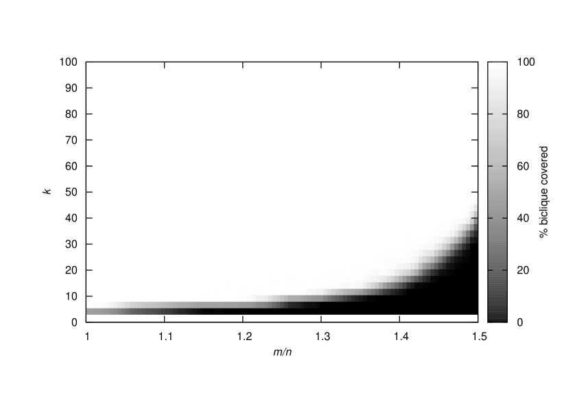
Figure 4: Results of experiments with our heuristic algorithm with strategy $S_{rand}^{2,3}$ and $|V_{v}|=100$. The horizontal axis represents the ratio $\frac{m}{n}$. The vertical axis represents the degree of vertices $v\in V_{c}(G)$. The more white pixel is, the more random graphs were covered by a bounded 2-biclique cover by the algorithm.

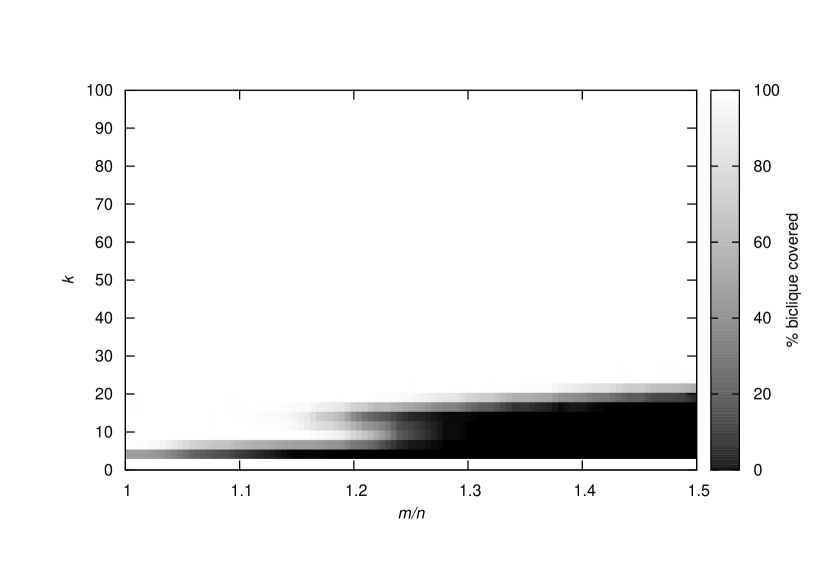
Figure 5: Results of experiments with our heuristic algorithm with strategy $S_{max}^{\infty}$ and $|V_{v}|=100$. The horizontal axis represents the ratio $\frac{m}{n}$. The vertical axis represents the degree of vertices $v\in V_{c}(G)$. The more white pixel is, the more random graphs were covered by a general bounded biclique cover by the algorithm.

We can observe a phase transition behaviour in the results of experiments on both strategies $S^{2,3}$ and $S^{\infty}$. As we can see on Figure 4 and Figure 5 there is a phase transition $r_{\frac{m}{n}}$ for a fixed ratio $\frac{m}{n}$. Most of random graphs $G\in\mathcal{G}_{m,n}^{k}$ with $k\geq r_{\frac{m}{n}}$ have a biclique cover and our heuristic algorithm will find it. However, since our heuristic is incomplete, it is not clear how many random graphs $G\in\mathcal{G}_{m,n}^{k}$ with $k\leq r_{\frac{m}{n}}$ have biclique cover.

In case of strategies with $S^{2,3}$ the most interesting case is when $\frac{m}{n}\leq 1.4$. As the ratio $\frac{m}{n}$ gets close to $1.5$ we can expect smaller percentage of graphs $G\in\mathcal{G}_{m,n}^{k}$ having a bounded 2-biclique cover, hence our heuristic algorithm fails to find one in most cases.

Strategy $S^{\infty}$ behaves very similarly to $S^{2,3}$ but it doesn’t have an upper limit to phase transition. As we can see, there is an interesting phenomenon on Figure 5 between $1.15$ and $1.25$. The strange shift is caused by using bigger bicliques by the algorithm.

As we can see from Table 3, for ratios $\frac{m}{n}$ smaller than $1.4$ it is better to use the algorithm with a heuristic for finding a bounded $2$-biclique cover. For bigger ratios $\frac{m}{n}$ it is better to use a heuristic for general bounded biclique cover. It would be also interesting to perform more experiments with bounded 3-biclique covers and observe if a similar phenomenon will occur on strategy $S^{\infty}$.

Table 6: Average running time (in $\mu s$) of experiments with our heuristic algorithm. Each column represents

	1			1.1			1.2			1.3			1.4			1.5
	$3$	$10$	$20$	$3$	$10$	$20$	$3$	$10$	$20$	$3$	$10$	$20$	$3$	$10$	$20$	$3$	$10$	$20$
$S_{rand}^{2,3}$	$3.01$	$4.66$	$1.18$	$3.01$	$6.03$	$34.25$	$3.01$	$7.83$	$51.26$	$3.01$	$9.09$	$61.68$	$3$	$10.34$	$69.61$	$3$	$11.8$	$77.25$
$S_{max}^{\infty}$	$3.01$	$4.78$	$1.18$	$3$	$6.47$	$19.35$	$3$	$7.95$	$30.44$	$3.01$	$8.99$	$38.88$	$3$	$9.96$	$44.9$	$3$	$11$	$49.58$

Average runtime of experiments on our heuristic can be seen in Table 6. For 3-CNF it has the same runtime for both strategies and all ratios of $\frac{m}{n}=1,\ldots,1.5$. This is because quite often an isolated vertex $v\in V_{c}$ was created during the work of Algorithm 1. Which means the algorithm failed quickly in many cases. Runtime of strategy $S^{2,3}$ which uses bounded bicliques in cover is much worse than unbounded strategy $S^{\infty}$. For $k$-CNF as $k$ grow, the difference gets bigger. Its because with unbounded strategy $S^{\infty}$ we admit bigger bicliques in cover and hence our heuristic Algorithm 1 will run fewer iterations of the main cycle and succeeds or fails faster than $S^{2,3}$.

5 Bounded Biclique SAT Encoding

We shall first describe the encoding of the problem of checking if a bipartite graph has a bounded biclique cover into SAT, then we will describe and evaluate the experiments we have performed to compare this approach with Algorithm 1. We will also describe the environment we have used to run the experiments.

5.1 Description of SAT Encoding

A valid biclique $B$ of a bipartite graph $G$ is a complete bipartite subgraph $B$ of the bipartite graph $G$ which follows the restriction on the size of the second partition. In particular, we require $|V_{c}(B)|<2^{|V_{v}(B)|}$. Let us consider a bipartite graph $G$ and $k\geq 1$, let us define

$$\mathcal{B}_{k}=\{B\mid\text{$B$ is a valid biclique of $G$ with $|V_{v}(B)|\leq k$}\}\text{.}$$

We also denote $\mathcal{B}_{\infty}$ the set of all bounded bicliques within the bipartite graph $G$ without restriction on the size of $V_{v}$. We would use set of bicliques $\mathcal{B}_{k}$ to check existence of a bounded k-biclique cover and $B_{\infty}$ to check existence of a general bounded biclique cover. We will encode problem of bounded ($k$-)biclique cover on a bipartite graph $G=(V_{v},V_{c},E)$. Let us fix $\mathcal{B}_{k}$ where $k$ is either a natural number, or $\infty$ and let us describe formula $\psi$ for a given graph $G$. With each biclique $B\in\mathcal{B}_{k}$ we associate a new variable $x_{B}$. Every assignment of boolean values to variables $x_{B}$, $B\in\mathcal{B}_{k}$ then specifies a set of bicliques. We want to encode the fact that the satisfying assignments of $\psi$ exactly correspond to bounded biclique covers of $G$. To this end we use the following constraints:

• For each vertex $v\in V_{v}$ we add to $\psi$ an at-most-one constraint on variables $x_{B}$, $v\in V_{v}(B)$. This encodes the fact that the first partitions of bicliques in the cover have to be pairwise disjoint. We use a straightforward representation of the at-most-one constraint with a quadratic number of negative clauses of size $2$.

• For each clause $C\in V_{c}$ we add to $\psi$ a clause representing an at-least-one constraint on variables $x_{b}$, $C\in V_{c}(B)$. This encodes the fact that each vertex of second partition belongs to a biclique in the cover.

5.2 Experimental Evaluation of Heuristic Algorithm

We can see that the number of variables in our encoding is equal to the number of all valid bicliques within the bipartite graph $G$. If we consider bicliques in $\mathcal{B}_{k}$ for a fixed $k$, then the number of valid bicliques $|\mathcal{B}_{k}|$ is polynomial in the size of $\varphi$ but it can be exponential in $i$ (for $\mathcal{B}_{\infty}$ the number can be exponential in the size of $\varphi$ as well). For this reason we tested the encoding only with bicliques in $\mathcal{B}_{2}$, thus checking bounded 2-biclique cover. For bigger bicliques the running times of experiments increased so much that we would not be able to repeat the tests enough times for a reasonable number of variables. We used the encoding described in Section 5.1 to check the success rate of our heuristic algorithm on random bipartite graphs and to check the phase transition for an existence of bounded biclique cover. We ran the experiments on $100$ random bipartite graphs $G\in\mathcal{G}^{k}_{m,n}$ with $n=40$ for combinations of $k=1,\ldots,8$ and the size of the second part $m=rn$ for $r=1.00,\ldots,1.25$ with step $0.05$. For each $k$ we tested random graphs only for the ratios around the expected phase transition as observed in the Table 3.

Table 7: Number of bipartite graphs with bounded biclique cover (found by Algorithm 1/ SAT finished with true/ SAT finished within time limit). If the three numbers are missing in a cell, no experiments were run with the corresponding configuration. In case of black cells we expect values $100/100/100$ and in case of white empty cells we expect $0/0/100$. See also the description within text.

	1	1.05	1.1	1.15	1.2	1.25
3	18/18/100	0/0/100
4	95/95/100	50/56/100	7/10/100	0/1/100	0/0/100
5	100/100/100	100/100/100	90/98/98	52/87/87	10/34/34	1/1/1
6		100/100/100	100/100/100	100/100/100	85/99/99	42/53/53
7				100/100/100	99/100/100	89/90/90
8						99/100/100

Table 8: Average runtime of Algorithm 1/average runtime of SAT on encoding in seconds.

	1	1.05	1.1	1.15	1.2	1.25
3	0.005/0.014	0.005/0.01
4	0.005/1.7	0.006/25	0.006/21	0.005/13	0.006/7
5	0.005/0.2	0.005/0.98	0.006/11	0.006/216	0.006/993	0.005/4589
6		0.006/0.4	0.006/2.4	0.006/50	0.006/838	0.006/3646
7				0.006/73	0.006/166	0.007/1666
8						0.006/272

Table 9: Average/maximum ratio between running time of Algorithm 1 and running time of SAT on encoding in seconds.

	1	1.05	1.1	1.15	1.2	1.25
3	0.52/2.16	0.58/2.39
4	0.13/1.05	0.02/0.40	0.002/0.06	0.001/0.005	0.001/0.009
5	0.25/1.13	0.06/1.16	0.007/0.12	0.002/0.096	$8\cdot 10^{-5}$/0.0008	$6\cdot 10^{-7}$/$6\cdot 10^{-7}$
6		0.12/0.88	0.023/0.30	0.003/0.095	0.0002/0.007	$8\cdot 10^{-5}$/0.0007
7				0.006/0.086	0.001/0.039	0.00018/0.0015
8						0.00026/0.0028

The results of experiments are contained in tables 7 to 9. All these tables have a similar structure. Each cell represents a single configuration (row corresponding by a value of $k$ and column corresponding to the ratio $m/n$ where $m$ denotes the number of clauses and $n=40$ denotes the number of variables). In Table 7 each cell contains three numbers separated with slashes. The first is the number of instances (out of $100$) on which Algorithm 1 successfully found a bounded biclique cover. The second is the number of instances on which the SAT solver successfully solved the encoding and answered positively. The third is the number of instances on which the SAT solver finished within time limit which was set to 4 hours for each instance. In some cells the values are missing, for these configurations we did not run any experiments, because they are far from the observed phase transition (see Table 3). In case of black colored cells we assume that the results would be $100/100/100$, in case of white colored cells we assume that the results would be $0/0/100$. The gray colored cells mark the borders of observed phase transition intervals of existence of bounded biclique cover, light gray corresponds to the results given by the SAT solver, dark gray to the results given by the heuristic which form an upper bound on the correct values. We can see that in most cases the number of positive answers given by Algorithm 1 is close to the number of positive answers given by the SAT solver. However, there are some cases where one of the approaches was more successful — namely in cases of $k=5,m/n=1.15,k=5$ and $k=5,m/n=1.2$. In the first case the SAT solver answered on $87$ instances positively while Algorithm 1 answered positively only on $52$ instances and in the second one SAT solver answered on $34$ positively and Algorithm 1 answered positively only on $10$ instances. However, in the second case we can see that SAT solver run over time limit (4 hours) in $\frac{2}{3}$ cases.

We also compared runtime of our heuristic algorithm and the SAT solver. As we can see in the Table 8 our heuristic algorithm is much faster in average case. Standard deviation of runtime of our heuristic algorithm is around $10^{-2}$ and the standard deviation of runtime of SAT solver is up to $10^{4}$ (where we have evaluated the average value and the standard deviation only on instances in which the SAT solver finished within the time limit 4 hours). These values are quite high compared to the running times. One of the reasons is perhaps the fact that the experiments were not run on a single computer, but on several comparable computers (see Section 5.3 for more details). Although in all cases on a single instance, the SAT solver and Algorithm 1 were run on a single computer and it makes thus sense to look at the ratio between the running times of these two. These are contained in Table 9. We can see that our heuristic is in most cases faster than the SAT solver using the encoding described in Section 5.1. Only for $k=3$ we can see that the maximum ratio is bigger than one. It means that in some cases SAT solver was faster than Algorithm 1, although not on average.

We can see from the results that on random $k$-CNF formulas Algorithm 1 has a success rate close to the one of the SAT based approach. A big advantage of Algorithm 1 is that it is much faster.

5.3 Experiments environment

Let us say more on the environment in which the experiments were run. We used Glucose parallel SAT solver [3, 9]. Our experiments were executed on grid computing service MetaCentrum NGI [1]. All experiments were run on a single processor machine (Intel Xenon, AMD Opteron) with 4 cores and frequency 2.20GHz-3.30GHz. On each random bipartite graph $G\in\mathcal{G}^{k}_{m,n}$, Algorithm 1 and the SAT solver were always run on the same computer. However, for the same configuration and different formulas, the experiments may have run on different computers. As we have noted in Section 5.2, this could be a reason of significantly high values of standard deviation of runtimes. The fact that the computer speed varied while the time limit for the SAT solver was still the same (4 hours) could have led to situations where the SAT solver would not finished, because it was run on a slower computer, and could potentially finish had it been run on a faster computer. We can see in Table 10 that most of the total 2000 instances finished within an hour, then only 26 finished between an hour and 2 hours, only 15 finished between 2 hours and 3 hours and only 9 finished between 3 hours and 4 hours. We can thus expect that the number of the border cases is similarly small. We can conclude that the variance in computer speeds had only minor influence on the number of SAT calls which finished within the time limit.

Table 10: Number of test cases finished in given interval.

$<$1h	1h-2h	2h-3h	3h-4h	$>$4h	total
1912	26	15	9	238	2200

6 Conclusion

The first result of our paper is that the experimental threshold of phase transition of property “being matched” of 3-CNFs is around 0.92 which is much higher than the theoretical lower bound 0.64 proved for 3-CNF by J. Franco and A.V. Gelder [10]. This can be seen in Figure 1. Moreover our experiments suggest that for $k\geq 6$ almost all formulas in $k$-CNF are matched (if they have at most as many clauses as variables).

We have also proposed a heuristic algorithm for finding a bounded ($k$-)biclique cover of a incidence graph $I(\varphi)$ of a given formula $\varphi$. In other words the algorithm tries to decide if $\varphi$ is biclique satisfiable. We suggested three different strategies for selecting a seed in our heuristic and compared them. We can deduce from figures 4 and 5 that the success rate of our heuristic algorithm exhibits a phase transition phenomenon similar to the case of matched formulas. The exact values are shown in Table 3. Our results suggest that it is better to use Algorithm 1 to find a 2-biclique cover using strategy $S_{rand}$ for ratios $\frac{m}{n}\leq 1.4$ where $m$ denotes the number of clauses and $n$ denotes the number of variables in a given formula. For higher ratios it is better not to restrict the size of the first part of the bicliques in the cover and to use strategy $S_{max}$.

Table 11: In this table we compare the phase transitions of property “being matched” and the success rate of Algorithm 1. Columns low and high have the same meaning as in tables 2 and 3

	matched		heuristic
	low	high	low	high
3-CNF	$0.909$	$0.929$	$0.9$	$0.93$
5-CNF	$0.99$	$0.995$	$1.02$	$1.08$

Table 11 presents a comparison of the results experiments on matched formulas with the results of experiments with Algorithm 1. As we can see, the success rate of Algorithm 1 exhibits a very similar phase transition to matched formulas. We can see that the low bound of the phase transition interval in case of matched formulas in $5$-CNF is $0.985$. In case of our algorithm the low bound of the phase transition interval is $1.02$. A formula can be matched only if the ratio $\frac{m}{n}$ of the number of clauses $m$ to a number of variables $n$ is at most $1$. According to the results of our experiments a random $k$-CNF with $k>5$ is matched with high probability even in case the ratio $\frac{m}{n}$ is $1$. However, for $7$-CNFs the low value of phase transition of our algorithm equals $1.14$ and for $k\geq 10$ it is even more than $1.3$, which means that if $\varphi$ is a formula in $10$-CNF with $n$ variables and at most $1.3n$ clauses, Algorithm 1 will most likely find a bounded biclique cover of the incidence graph of $\varphi$. These results are summarized in Table 3.

Our heuristic algorithm is not complete, in particular, it can happen that a formula is biclique satisfiable, but Algorithm 1 is unable to detect it. It means that we can only trust a positive answer of the algorithm. We have compared our heuristic with a SAT based approach which can also check that a formula is not biclique satisfiable. We can see in Table 7 that formulas on which Algorithm 1 fails to answer correctly, are concentrated around the observed phase transition, and that the algorithm answers correctly in most cases for other configurations. We can say that the success rate of Algorithm 1 is not far from the complete SAT based method. Moreover, as we can see in tables 8 and 9, our heuristic is significantly faster than a SAT solver on the encoding we have described.

7 Future work

There is still some space to improve our results.

We can try to develop better heuristics for selecting a seed and other steps of our algorithm. For example we can use other sizes of bicliques than $K_{1,1},K_{2,3}$ and unbounded ones. It would also be interesting to test our heuristic on $k$-biclique cover for $k>2$. Additionally a deterministic selection heuristic of vertices in function restrictSeed could improve the success rate of our heuristic Algorithm 1.

It would be also interesting to find a better SAT encoding of the problem which would allow us to run experiments on bigger instances of input formulas.

The last question is, can be our heuristic algorithm and SAT encoding generalized to var-satisfiability?

References

- [1] Metacentrum grid computing (June 2017), https://metavo.metacentrum.cz/en/
- [2] Aharoni, R., Linial, N.: Minimal non-two-colorable hypergraphs and minimal unsatisfiable formulas. Journal of Combinatorial Theory, Series A 43(2), 196 – 204 (1986). https://doi.org/http://dx.doi.org/10.1016/0097-3165(86)90060-9, http://www.sciencedirect.com/science/article/pii/0097316586900609
- [3] Audemard, G., Simon, L.: The glucose sat solver (June 2017), http://www.labri.fr/perso/lsimon/glucose/
- [4] Bollobás, B.: Modern Graph Theory, Graduate Texts in Mathematics, vol. 184. Springer (1998)
- [5] Cheeseman, P., Kanefsky, B., Taylor, W.M.: Where the really hard problems are. In: Proceedings of the 12th International Joint Conference on Artificial Intelligence - Volume 1. pp. 331–337. IJCAI’91, Morgan Kaufmann Publishers Inc., San Francisco, CA, USA (1991), http://dl.acm.org/citation.cfm?id=1631171.1631221
- [6] Connamacher, H.S., Molloy, M.: The satisfiability threshold for a seemingly intractable random constraint satisfaction problem. CoRR abs/1202.0042 (2012), http://arxiv.org/abs/1202.0042
- [7] Cook, S.A.: The complexity of theorem-proving procedures. In: Proceedings of the Third Annual ACM Symposium on Theory of Computing. pp. 151–158. STOC ’71, ACM, New York, NY, USA (1971). https://doi.org/10.1145/800157.805047, http://doi.acm.org/10.1145/800157.805047
- [8] Dubois, O., Boufkhad, Y., Mandler, J.: Typical random 3-sat formulae and the satisfiability threshold. In: Proceedings of the Eleventh Annual ACM-SIAM Symposium on Discrete Algorithms. pp. 126–127. SODA ’00, Society for Industrial and Applied Mathematics, Philadelphia, PA, USA (2000), http://dl.acm.org/citation.cfm?id=338219.338243
- [9] Eén, N., Sörensson, N.: The minisat (June 2017), http://minisat.se/
- [10] Franco, J., Gelder, A.V.: A perspective on certain polynomial-time solvable classes of satisfiability. Discrete Applied Mathematics 125(2–3), 177 – 214 (2003). https://doi.org/http://dx.doi.org/10.1016/S0166-218X(01)00358-4, http://www.sciencedirect.com/science/article/pii/S0166218X01003584
- [11] Gent, I.P., Walsh, T.: The SAT phase transition. In: Proceedings of the 11th European Conference on Artificial Intelligence. pp. 105–109. John Wiley & Sons (1994)
- [12] Heydari, M.H., Morales, L., o. S. Jr., C., Sudborough, I.H.: Computing cross associations for attack graphs and other applications. In: System Sciences, 2007. HICSS 2007. 40th Annual Hawaii International Conference on. pp. 270b–270b (Jan 2007). https://doi.org/10.1109/HICSS.2007.141
- [13] Hopcroft, J.E., Karp, R.M.: An algorithm for maximum matchings in bipartite graphs. SIAM Journal on computing 2(4), 225–231 (1973)
- [14] Lovász, L., Plummer, M.D.: Matching Theory. North-Holland (1986)
- [15] Mitchell, D., Selman, B., Levesque, H.: Hard and easy distributions of sat problems. In: Proceedings of the 10th National Conference on Artificial Intelligence (AAAI-92). pp. 459–465. San Jose, CA, USA (1992)
- [16] Szeider, S.: Generalizations of matched CNF formulas. Annals of Mathematics and Artificial Intelligence 43(1), 223–238 (2005). https://doi.org/10.1007/s10472-005-0432-6, http://dx.doi.org/10.1007/s10472-005-0432-6
- [17] Tovey, C.A.: A simplified NP-complete satisfiability problem. Discrete Applied Mathematics 8(1), 85 – 89 (1984). https://doi.org/http://dx.doi.org/10.1016/0166-218X(84)90081-7, http://www.sciencedirect.com/science/article/pii/0166218X84900817