X-ray Luminosity Function of Quasars at 3<z<5 from XMM-Newton Serendipitous Survey Data

Аннотация

The X-ray luminosity function of distant ($3<z<5.1$) unabsorbed quasars has been measured. A sample of distant high-luminosity quasars ($10^{45}\leq L_{{\rm X},2-10}<7.5\times 10^{45}$ erg/s in the 2–10 keV energy band) from the catalog given in Khorunzhev et al. (2016) compiled from the data of the 3XMM-DR4 catalog of the XMM-Newton serendipitous survey and the Sloan Digital Sky Survey (SDSS) has been used. This sample consists of 101 sources. Most of them (90) have spectroscopic redshifts $z_{\mbox{\scriptsize spec}}\geqslant 3$. The remaining ones are quasar candidates with photometric redshift estimates $z_{\mbox{\scriptsize phot}}\geqslant 3$. The spectroscopic redshifts of eight sources have been measured with АZT-33IK and BTA telescopes. Owing to the record sky coverage area ($\simeq 250$ sq. deg at X-ray fluxes $\sim 10^{-14}$ erg/s/cm² in the 0.5-2 keV), from which the sample was drawn, we have managed to obtain reliable estimates of the space density of distant X-ray quasars with luminosities $L_{{\rm X},2-10}>2\times 10^{45}$ erg/s for the first time. Their comoving space density remains constant as the redshift increases from $z=3$ to $z=5$ to within a factor of 2. The power-law slope of the X-ray luminosity function of high-redshift quasars in its bright end (above the break luminosity) has been reliably constrained for the first time. The range of possible slopes for the quasar luminosity dependent density evolution model is $\gamma_{2}=2.78^{+0.00}_{-0.04}\pm 0.20$, where initially the lower and upper boundaries of $\gamma_{2}$ with the remaining uncertainty in the detection completeness of X-ray sources in SDSS, and subsequently the statistical error of the slope are specified.

2018448-9500[521] 524.7

10.11.2017 г.

1 Introduction

A reliable measurement of the X-ray luminosity function of high-luminosity active galactic nuclei (AGNs, hereafter quasars) and its evolution at $z\gtrsim 3$ is one of the most important components of the research on the growth history of supermassive black holes and the evolution of massive galaxies in the Universe. The samples of XMM-Newton and Chandra extragalacitc X-ray surveys (representative fluxes $F_{{\rm X},0.5-2}\lesssim\leavevmode\nobreak\ 10^{-15}$ erg/s/cm² and areas about one sq. deg) turn out to be insufficiently large for the evolution of distant quasars to be studied (Civano , 2012; Vito , 2014). The addition of sources from shallower extragalactic surveys ($F_{{\rm X},0.5-2}\sim 10^{-14}$–$10^{-13}$ erg/s/cm²) covering much larger areas (tens of square degrees Ueda et al. 2014; Aird et al. 2015; Georgakakis 2015) improves the situation.

Vito (2014) constructed and extensively studied the luminosity function of quasars at $z>3$ with luminosities $L_{{\rm X},2-10}<10^{45}$ erg/s in the 2–10 keV band based on the combined data of several deep X-ray surveys with a total area $\simeq 3.3$ sq. deg. Using data from the XMM-XXL survey with an area of 18 sq. deg (typical fluxes of sources $F_{{\rm X},0.5-2}\simeq 5\times 10^{-15}$ erg/s/cm², Menzel 2016), Georgakakis (2015), obtained statistically significant estimates of the quasar luminosity funcion at $z>3$ for even higher luminosities ($L_{{\rm X},2-10}\gtrsim 10^{45}$ erg/s).

Ueda et al. (2014) studied the evolution of the X-ray luminosity function of AGNs based on the collection of data from a large set of X-ray surveys, including the ROSAT all-sky survey. The ROSAT sample of sources includes several quasars with a very high luminosity ($L_{{\rm X},2-10}>10^{46}$ erg/s) at $z>3$, which allowed the space density of such very luminous and distant quasars to be constrained. This estimate turned out to be in agreement with the predictions of the empirical luminosity function model obtained from samples of sources with a much lower luminosity ($L_{X,2-10}<10^{45}$ erg/s).

Kalfountzou et al. (2014) compiled a catalog of quasars at $z>3$ on an area of $\simeq 33$ sq. deg based on the archival data of individual nonoverlapping Chandra pointings over the entire time of its operation. Using this catalog, they were able to estimate the space density of distant quasars with luminosities $L_{X,2-10}>5\times 10^{44}$ erg/s and to exclude some of the empirical luminosity function models. However, the size of this sample is still insufficient for a detailed study of the population of most luminous ($L_{{\rm X},2-10}>10^{45}$ erg/s) and distant ($z>3.5$) quasars.

The data from the XMM-Newton X-ray telescope accumulated over 15 years constitute a serendipitous sky survey (Watson , 2009) with a total coverage of $\sim$800 sq. deg and a sensitivity $F_{{\rm X},0.5-2}\sim 5\times 10^{-15}$ erg s^-1 cm^-2 (the 3XMM-DR4 fourth data release of serendipitous source catalog, Watson , 2009).

Based on these data, one can produce an X-ray sample of quasars at $z>3$ that exceeds the existing samples by several times (Kalfountzou et al., 2014; Georgakakis , 2015) and obtain more rigorous constraints on the luminosity function model parameters. This is the goal of our paper.

We made an attempt to find new candidates for distant quasars among the X-ray sources of the 3XMM-DR4 catalog as described in (Khorunzhev , 2016, 2017a). Our goal was to obtain a sample of X-ray quasars at $z>3$ as complete as possible in XMM-Newton serendipitous survey fields at Galactic latitudes $|b|>20^{\circ}$ using photometric data from the Sloan Digital Sky Survey (SDSS, Alam , 2015) as well as the infrared 2MASS (Cutri , 2003) and WISE (Wright , 2010). The total area of the overlap between these surveys is 300 sq. deg.

The photometric redshift estimates ($z_{\mbox{\scriptsize phot}}$) had been done by khorunzhev16AA and a catalog (K16) of 903 candidates for distant quasars (presumably of type 1) selected by photometric redshift had been compiled. The catalog includes both previously known quasars (with measured spectroscopic redshifts $z_{\mbox{\scriptsize spec}}>3$) and new quasar candidates (with photometric redshift estimates $z_{\mbox{\scriptsize phot}}>2.75$).

The additional table of the K16  catalog presents 63 known X-ray quasars with $z_{\mbox{\scriptsize spec}}>3$ that did not pass the photometric selection of quasar candidates. The first results of our spectroscopic identification of new quasar candidates from the K16 catalog, based on which we made a quantitative estimate of the purity of this catalog, are presented in Khorunzhev (2017a), Khorunzhev (2017b). The additional selection was shown to provide an increase in the number of new sources at $z>3$ relative to the existing spectroscopic sample of quasars: by $\sim 20$% for optically bright ($\mbox{z}^{\prime}<20$) and X-ray ($L_{{\rm X},2-10}\gtrsim 10^{45}$ erg/s) luminous sources and by $\sim 50$% for fainter sources.

In this paper we use data from the K16 catalog to measure the space density of luminous ($L_{{\rm X},2-10}>10^{45}$ erg/s) quasars at $z>3$ and to obtain rigorous constraints on the slope of the luminosity function $\gamma_{2}$ in its bright end. In our calculations we used the following cosmological constants, the same as those in Vito et al. (2014), whose results are actively used below: $H_{0}=70$ km/s/Mpc, $\Omega_{\rm m}=0.27$, $\Omega_{\lambda}=0.73$.

2 THE SAMPLE

To construct the X-ray luminosity function, we used a sample of 205 sources composed of the parts of two catalogs: 101 sources with luminosities $L_{{\rm X},2-10}\geq 10^{45}$ erg/s from the catalog by Khorunzhev (2016) and 104 unabsorbed sources with $L_{{\rm X},2-10}<1.1\times 10^{45}$ erg/s from the catalog by Vito (2014).

2.1 The Subsample of Luminous Quasars from the K16 Catalog

To investigate high-luminosity ($\geq 10^{45}$ erg/s) quasars, we used the K16 catalog of quasars and candidates for distant quasars (Khorunzhev , 2016). We considered both objects from the main catalog and sources from the additional table of known quasars with $z_{\mbox{\scriptsize spec}}>3$ that did not pass the photometric selection. The sources that were XMM-Newton pointing targets and the blazar 3XMM J142437.8+225601 were excluded.

As a result, we selected 101 sources with 2–10 keV X-ray luminosities $L_{{\rm X},2-10}\geq 10^{45}$ erg/s in the source’s rest frame. The luminosity was calculated via the measured 0.5-2 keV flux under the assumption of a power-law spectrum with a slope $\Gamma$=1.8 without absorption (just as in Vito 2014 for unabsorbed sources). In the case where an object had no spectroscopic redshift, the luminosity was calculated from $z_{\mbox{\scriptsize phot}}$, the photometric redshift estimate. As a result of the selection by luminosity, all sources of the K16 subsample turned out to have an X-ray flux above 4$\times 10^{-15}$ erg/s/cm². The distribution of sources in X-ray flux, luminosity, and redshift is shown in Fig. 1. The list of sources is given in Table LABEL:tab:catlum.

For 82 of the 101 sources $z_{\mbox{\scriptsize spec}}\geq 3$ was known at the time of K16 publication. The sample also includes 8 spectroscopically confirmed candidates with $z_{\mbox{\scriptsize spec}}\geq 3$ whose spectra were taken with the 1.6-m АЗТ-33ИК telescope at the Sayan Solar Observatory of the Institute of Solar–Terrestrial Physics, the Siberian Branch of the Russian Academy of Sciences, and the 6-m BTA telescope at the Special Astrophysical Observatory of the Russian Academy of Sciences during our program of searching for distant quasars (Khorunzhev , 2017a, b; G. Khorunzhev , 2019). The remaining 11 objects are quasar candidates with photometric redshift estimates $z_{\mbox{\scriptsize phot}}\geq 3$ unambiguously identified in the optical band (without the "D" flag in the K16 catalog). The source 3XMM J114816.0+525900 ($z_{\mbox{\scriptsize spec}}=3.173$) has the highest luminosity $L_{{\rm X},2-10}=7.4\times 10^{45}$ erg/s. 3XMM J022112.5-034251 is the most distant source $z_{\mbox{\scriptsize spec}}=5.011$, $L_{{\rm X},2-10}=1.9\times 10^{45}$ erg/s. Our sample contains several times more X-ray luminous quasars than the previously used data from smaller area X-ray surveys (Kalfountzou et al., 2014; Vito , 2014; Aird et al., 2015; Georgakakis , 2015).

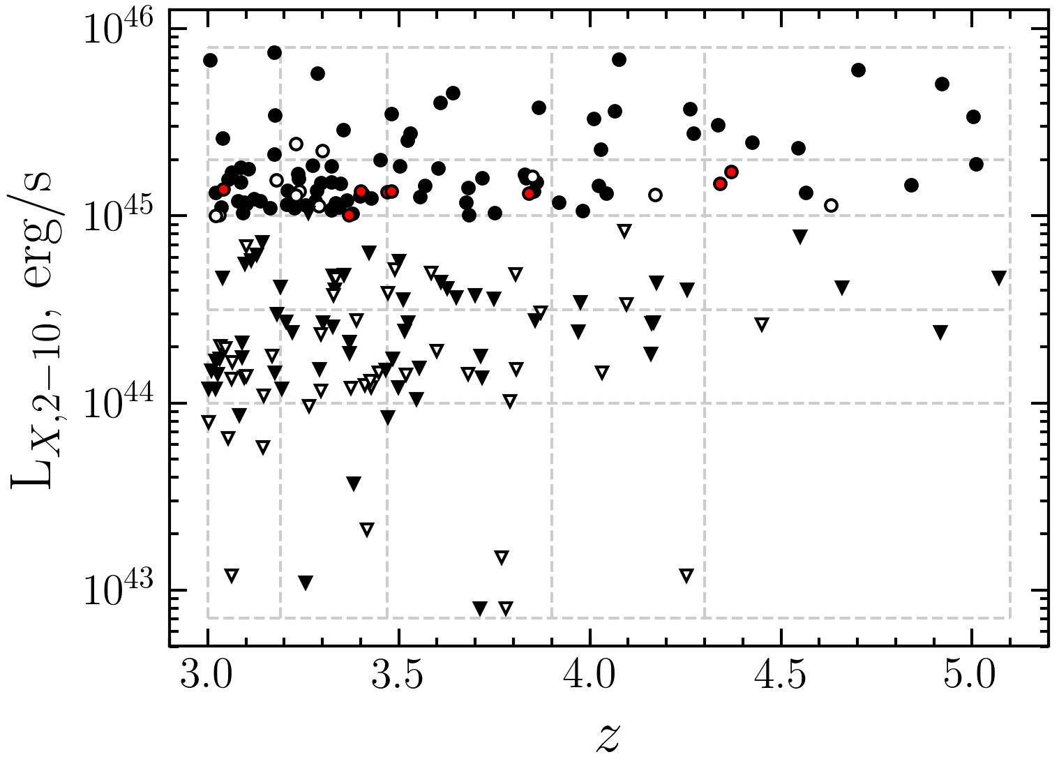
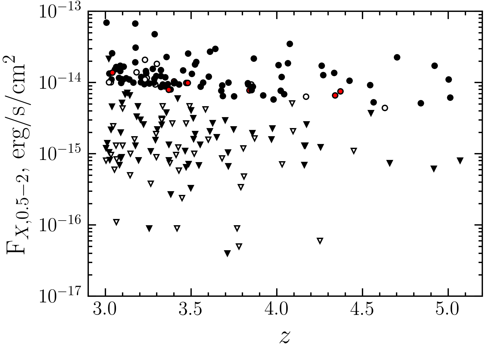
Рис. 1: Top: X-ray luminosities (2–10 keV in the objects’s rest frame) and redshifts of the quasars from the K16 (circles) and V14U (triangles) subsamples. The vertical and horizontal dashed lines indicate the boundaries of the $\Delta\log L$–$\Delta z$ bins for constructing the binned (nonparametric) luminosity function by the $1/V_{\rm max}$ method. Bottom: X-ray fluxes (0.5–2 кэВ) and redshifts of the sources from the same subsamples. The filled symbols indicate the objects with spectroscopic redshifts ($z_{\mbox{\scriptsize spec}}$). The objects from the K16 catalog whose spectroscopic redshifts were measured already after the publication of the catalog (Khorunzhev , 2017a, b; G. Khorunzhev , 2019) are highlighted by the red color. The open symbols indicate the objects for which there are only photometric redshift estimates ($z_{\mbox{\scriptsize phot}}$).

Our sample consists of unabsorbed or weakly absorbed X-ray quasars with an intrinsic absorption column density $N_{\rm H}<10^{23}$ cm^-2. This is evidenced by the distribution of sources in X-ray hardness ratio (3XMM-DR4 data) and redshift presented in Fig. 2. The hardness ratio ($SC_{HR2}=(H-S)/(H+S)$) is defined via the photon count rates in the 1–2 keV (H) and 0.5–1 keV (S) bands. For comparison, Fig. 2 shows the redshift dependences of the hardness ratio expected for a power-law spectrum with a slope $\Gamma=1.8$ and various absorption column densities. We see that only a few sources from the sample would have $N_{\rm H}\simeq 10^{23}$ cm^-2. The rest should have a lower intrinsic absorption.

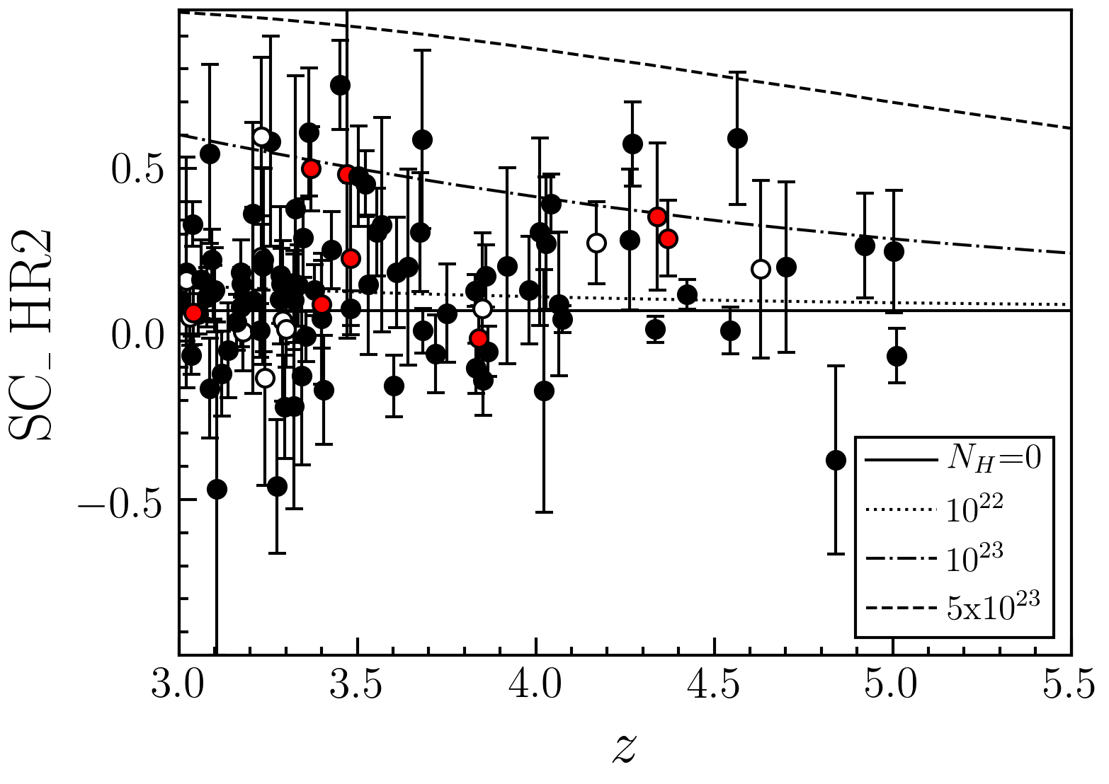
Рис. 2: Distribution of K16 sources in X-ray hardness ratio (defined via the 1–2 and 0.5–1 keV fluxes, see the text) and redshift. The quasars with known $z_{\mbox{\scriptsize spec}}$ are indicated by the black symbols; the objects from the K16 catalog whose spectroscopic redshifts were measured already after the publication of the catalog (Khorunzhev , 2017a, b; G. Khorunzhev , 2019) are highlighted by the red color; the objects for which only $z_{\mbox{\scriptsize phot}}$ are known are designated by the open symbols. The lines indicate the dependence of the hardness ratio on redshift and intrinsic absorption column density for a power-law spectrum with $\Gamma=1.8$.

The absence of heavily absorbed X-ray sources in the sample is related to the method of selecting distant quasars in the optical band. When compiling the K16 catalog based on shallow broadband photometry, we selected type 1 quasars with an ultraviolet excess (in the quasar’s rest frame) and an absorption gain behind the Ly$\alpha$ line. The same selection effect is described, for example, in Kalfountzou et al. (2014), where the fraction of luminous quasars with absorption $N_{\rm H}>10^{23}$ cm^-2 was about 10% due to a similar selection method, and Vito (2014), where from Table 1 it can be seen how the fraction of absorbed quasars drops with decreasing sensitivity of X-ray and optical surveys.

2.2 The Subsample of Fainter Quasars from the Paper by Vito et al.

The quasar luminosity function has the form of a power law with a break (Boyle 1988; Miyaji  2000; see Eq. (2) below). A sample spanning a wide luminosity range is needed to determine all parameters of the luminosity function model. The region near the break in the luminosity function, where the power-law slope changes, is especially important. All objects in the K16 catalog have luminosities higher than the break luminosity ($L_{{\rm X},2-10}\simeq 4\times 10^{44}$ erg/s; Vito 2014). Therefore, it was decided to supplement the K16 list of luminous quasars by the sample from Vito (2014), which contains many objects near the break luminosity.

The catalog of X-ray quasars at $z>3$, based on which we constructed the luminosity function, is presented in the paper by Vito (2014). Almost all of the sources have spectroscopic measurements or reliable estimates of the redshift obtained from deep photometric survey data in medium-band filters. Therefore, it is convenient to use the sample by Vito (2014) to extend K16 to lower luminosities. From the catalog Vito (2014) it is easy to extract the V14U subsample of unabsorbed sources (absorption column density $N_{\rm H}\leq 10^{23}$ cm^-2) for a better correspondence to the K16 sample.

The original sample by Vito (2014) consists of 141 X-ray sources at redshifts $3<z<5.1$ and was obtained from the data of four deep X-ray surveys: Chandra Deep Field South (CDFS, Xue 2011, Chandra Cosmos Survey (C-COSMOS, Elvis 2009), XMM-Newton Cosmos Survey (XMM-Cosmos, Hasinger 2007), and Subaru/XMM-Newton Deep Survey (SXDS, Ueda 2008). In these surveys the optical identification completeness of X-ray sources is higher than 95%. The total area is 3.3 sq. deg. A total of three sources have 2-10 keV luminosities $\geq 10^{45}$ erg/s. Only one of them is unabsorbed.

The subsample of 104 unabsorbed sources (V14U) used in our paper consists of quasars with luminosities $8\times 10^{42}<L_{{\rm X},2-10}<1.04\times 10^{45}$ erg/s. The source ID 5120 was excluded from the XMM-COSMOS survey, because it is a star (Lilly , 2007). The most distant source ID 2220 ($z_{\mbox{\scriptsize spec}}=5.07$, $L_{{\rm X},2-10}=4.7\times 10^{44}$ erg/s) was found in the C-COSMOS survey (Elvis , 2009). The most luminous source ID 926 ($L_{{\rm X},2-10}=1.04\times 10^{45}$ erg/s, $z_{\mbox{\scriptsize spec}}=3.264$) was found in the SXDS survey (Ueda , 2008). In Fig. 1 the X-ray fluxes, luminosities, and redshifts of the sources from the V14U subsample are compared with the corresponding characteristics of the sources from the K16 subsample.

3 THE SURVEY AREA

To calculate the space density of sources, we need to know how the sky coverage area of the X-ray survey changes with sensitivity. For the V14U subsample of unabsorbed low-luminosity sources we took the corresponding area for unabsorbed sources from Vito (2014) (see Fig. 3).

To calculate the area of the XMM-Newton serendipitous survey, we selected the pointings (OBSID) that were used to construct the 3XMM-DR4 catalog of X-ray sources (Watson , 2009) and were previously used by us (Khorunzhev , 2016) to roughly estimate the survey area: the sources must be at Galactic latitudes $|b|>20^{\circ}$ and fall into the SDSS region. Using the utility task esensmap of the XMM-Newton Science Analysis System, we constructed the sensitivity maps of individual pointings (in counts/s/PSF) for the detection threshold $det_{\rm ML}>6$ in the range 0.2-12 keV for the total exposure of all the detectors involved in this pointing. The original 3XMM-DR4 catalog of X-ray sources was compiled precisely with this detection threshold ($det_{\rm ML}>6$). In the case where the nearby pointings overlapped to form a mosaic, we chose fields from the pointing with the best sensitivity to construct the sensitivity map in the overlapping region.

When the 3XMM-DR4 catalog of sources was compiled, the counts from all the operating detectors for an individual pointing were taken into account. Each mode of operation of the XMM-Newton detectors is characterized by its count rate-to-flux conversion factor. To convert the sensitivity map from counts/s to erg/s/cm² (the 0.2-12 keV band), we calculated the effective conversion factor from the following formula:

$$\langle ECF\rangle=\dfrac{\sum\limits_{i=1}^{N_{\rm det}}EXP_{i}\times ECF_{i}}{\langle EXP\rangle},$$ (1)

$$\langle EXP\rangle=\frac{1}{N_{\rm det}}\sum\limits_{i=1}^{N_{\rm det}}EXP_{i},$$

where $N_{\rm det}$ — is the number of operating detectors in a given pointing, $EXP_{i}$ is the exposure map of the i-th detector, $ECF_{i}$ is the count rate-to-flux conversion factor (the 0.2–12 keV band) for the mode of operation of $i$-th detector, $\langle EXP\rangle$ is the mean exposure time. The sensitivity map was then divided by the map of the effective count rate-to-flux conversion factor $\langle ECF\rangle$. The fluxes were converted from the 0.2-12 keV band to the 0.5-2 keV band of interest to us by assuming a power-law spectrum of sources with a slope $\Gamma=1.7$ and absorption $N_{H}=10^{20}$ cm^-2 (roughly corresponding to the absorption in the Galactic interstellar medium). We used precisely $\Gamma=1.7$, because the tabulated count rate-to-flux conversion factors for the XMM-Newton bands are given for this slope. For all of the chosen fields we then obtained the cumulative number distribution of pixels (with a flux below the specified one) and constructed the dependence of the survey area on X-ray flux (see Fig. 3).

The total area of the overlap between 3XMM-DR4 and SDSS is 320 sq. deg, which is almost a factor of 100 larger than the total area of the V14U survey from Vito (2014).

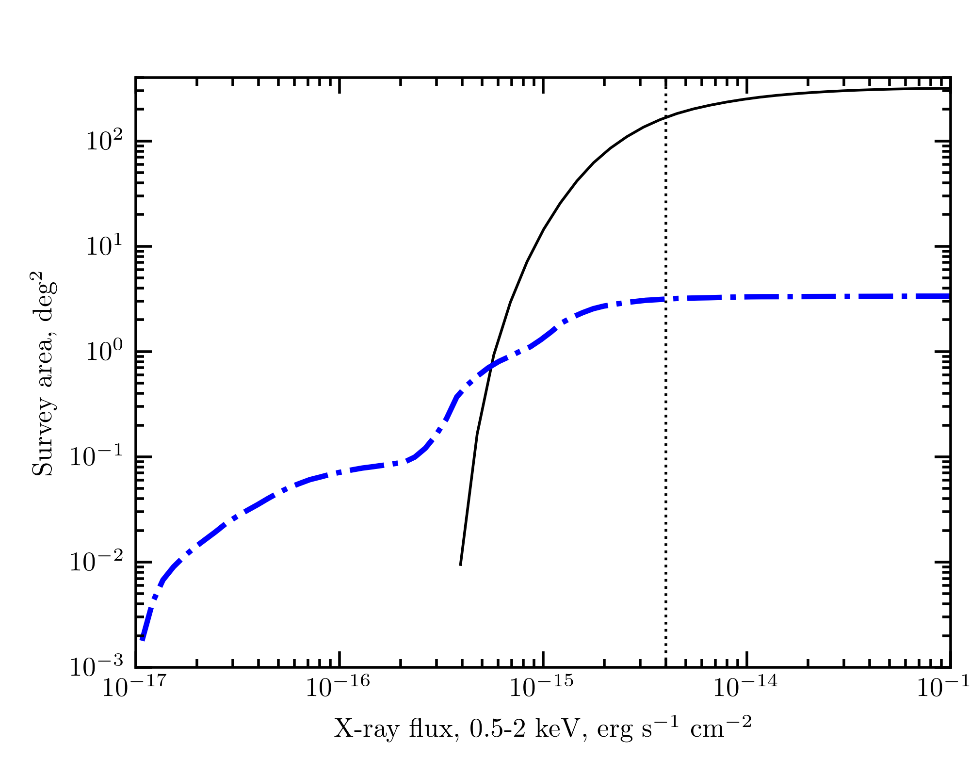
Рис. 3: The 3XMM-DR4 survey area (black solid line) and total area of deep surveys for unabsorbed sources (Vito 2014, the blue dash-dotted line). The vertical dotted line marks the lower boundary the 0.5–2 keV X-ray flux $4\times 10^{-15}$ erg/s/cm² for the K16 subsample of objects with $L_{{\rm X},2-10}>10^{45}$ erg/s.

4 THE SDSS IDENTIFICATION COMPLETENESS OF X-RAY SOURCES

To obtain trustworthy photometric reshifts $z_{\mbox{\scriptsize phot}}$ when constructing the K16 catalog (Khorunzhev , 2016), we used only reliable optical sources, with an error of the apparent magnitude $\Delta\mbox{z}^{\prime}<0.2$ in the SDSS  $\mbox{z}^{\prime}$ band, corresponding to an effective detection threshold $\mbox{z}^{\prime}\simeq 20.5$. Fainter sources were not included in the K16 catalog. This could skew the sample toward optically luminous quasars (see Fig. 4). This figure shows the distribution of type 1 quasars from the K16 sample in X-ray flux and apparent magnitude in the SDSS $\mbox{z}^{\prime}$ band.

For comparison, Fig. 4 shows the unabsorbed sources from the V14U subsample that has an almost 100% optical identification completeness. The apparent magnitudes of the X-ray sources in the $\mbox{z}^{\prime}$ band were taken from Civano (2012); Capak (2007) for C-COSMOS and XMM-COSMOS respectively, and Akiyama (2015) for SXDS. The magnitudes from the GOODS (Giavalisco , 2004) and GEMS (Caldwell , 2008) photometric surveys in the z850 filter, whose range roughly coincides with the SDSS $\mbox{z}^{\prime}$ band, were used for the CDFS survey (Xue , 2011).

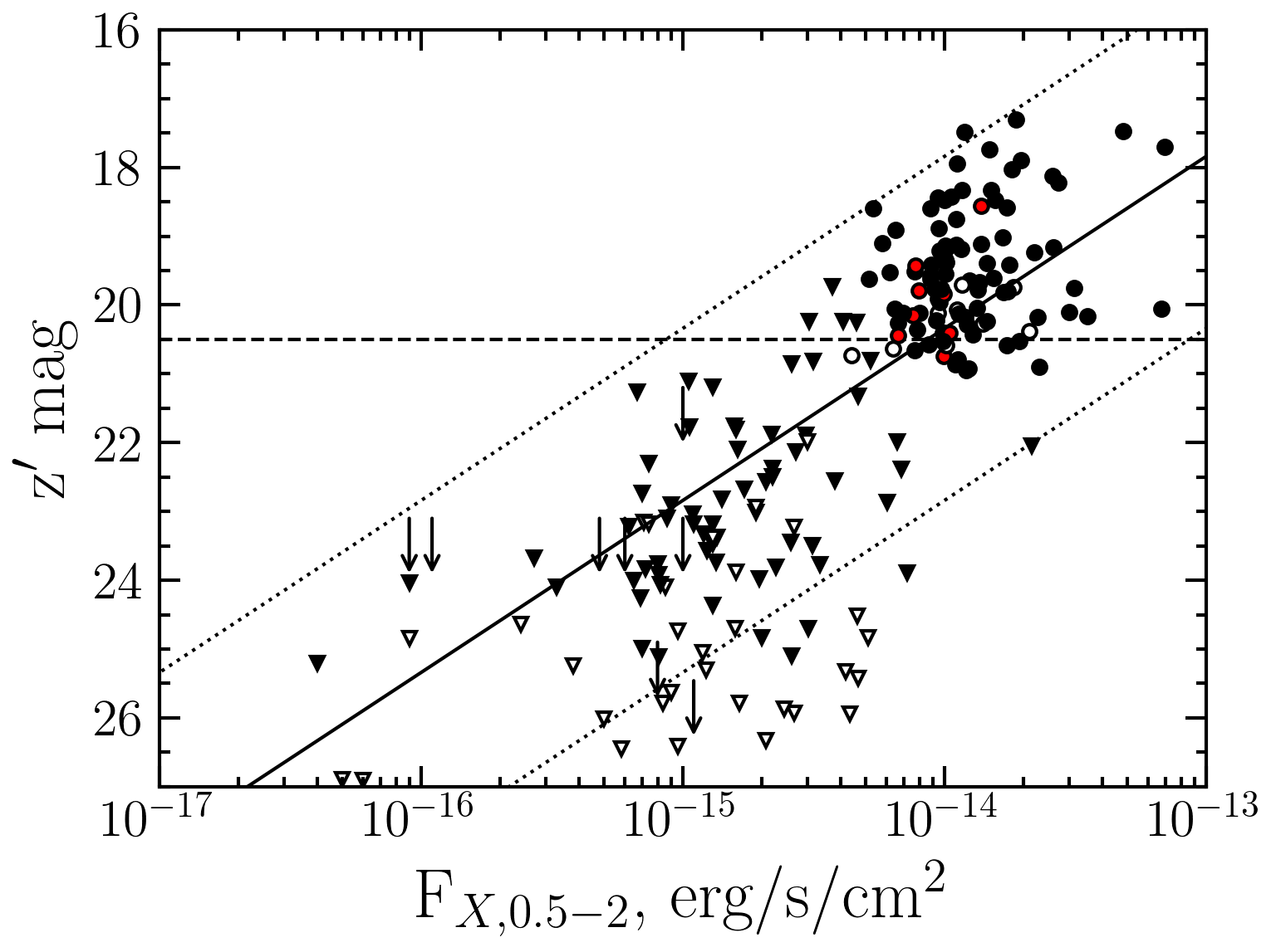
Рис. 4: Apparent $\mbox{z}^{\prime}$ magnitudes and X-ray (0.5-2 keV) fluxes of the sources from the K16 (circles) and V14U (triangles) subsamples. The filled symbols indicate the objects with spectroscopic redshifts ($z_{\mbox{\scriptsize spec}}$); the objects from the K16 catalog for which the spectroscopic redshifts were measured already after the publication of the catalog (Khorunzhev , 2017a, b; G. Khorunzhev , 2019) are red highlighted. The open symbols indicate the objects for which there are only photometric redshift estimates ($z_{\mbox{\scriptsize phot}}$). The arrows mark the lower limits on $\mbox{z}^{\prime}$. The solid line indicates the ratio of the X-ray and optical fluxes $f_{X}/f_{O}=1$; the dotted lines indicate $f_{X}/f_{O}=0.1$ and $f_{X}/f_{O}=10$. The horizontal dashed line indicates the effective threshold of the K16 catalog $\mbox{z}^{\prime}=20.5$.

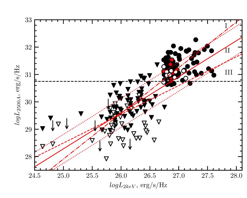
Рис. 5: Relation between monochromatic optical luminosity $L_{2500\mathring{A}}$ at wavelength 2500 Å and monochromatic X-ray luminosity $L_{\rm 2\,keV}$ at energy 2 keV for the K16 and V14U  subsamples. The designations are the same as those in Fig. 4. The red solid line labeled by "II" indicates the $L_{\rm 2\,keV}$–$L_{2500\mathring{A}}$ relation from Lusso (2010), which was taken as a basis in calculating the correction for incompleteness. The red dash–dotted and dashed lines labeled by "I" and "III" indicate other $L_{\rm 2\,keV}$–$L_{2500\mathring{A}}$ relations from Lusso (2010) that are used as the minimum and maximum corrections for incompleteness. The dotted lines indicate the $\pm 0.4$ scatter for the $L_{\rm 2\,keV}$–$L_{2500\mathring{A}}$ relation II. The horizontal dashed line indicates the threshold luminosity $L_{2500\mathring{A}}$ that a source with an apparent magnitude $\mbox{z}^{\prime}=20.5$ at redshift $z=3$ whose spectrum is described by the template from Vanden Berk  (2001) will have.

It can be seen from Fig. 4 that the X-ray-to-optical flux ratio for most of the K16 sources is less than unity ($f_{X}/f_{O}<1$), while most of the objects from the V14U sample have $f_{X}/f_{O}>1$. This can be related in part to the known nonlinear correlation between the optical and X-ray luminosities of quasars: the higher the bolometric luminosity of an object, the smaller the ratio $f_{X}/f_{O}$ (see, e.g., Lusso 2010, 2017) The fact that the threshold $\mbox{z}^{\prime}\simeq 20.5$ used in constructing the K16  catalog turns out to be insufficient for the detection of all high-luminosity X-ray quasars at $z>3$ is apparently more important.

4.1 The Method of Calculating the Correction for Incompleteness

The completeness of quasars in the K16 subsample cannot be estimated using the observational data of X-ray surveys with an area of $\sim 20$ sq. deg, for example, XMM-XXL. The size of such surveys is too small to detect a sufficient number of distant quasars with luminosities $\geq 10^{45}$ erg/s. Therefore, we used the relation between the X-ray, $L_{\rm 2\,keV}$, and optical, $L_{2500\mathring{A}}$, monochromatic luminosities of type 1 quasars (Lusso , 2010; Marchese , 2012) to determine the missed fraction of X-ray quasars with an apparent magnitude $\mbox{z}^{\prime}>20.5$.

Lusso (2010) used a subsample of type 1 quasars from the deep XMM-COSMOS survey to investigate the $L_{\rm 2\,keV}$–$L_{2500\mathring{A}}$ relation. In this sample 60% of the sources have spectroscopically confirmed redshifts. Most of the quasars at $z>3$ from the sample by (Lusso , 2010) are present in the V14U sample. Subsequently, Marchese (2012) obtained similar results for a spectroscopically complete sample of optically luminous quasars selected in the X-ray and ultraviolet bands.

We considered three variants of the $L_{\rm 2\,keV}$–$L_{2500\mathring{A}}$ relation:

I $$:\log L_{2500\mathring{A}}=1.669\log L_{\rm 2\,keV}-13.815,$$

II $$:\log L_{2500\mathring{A}}=1.316\log L_{\rm 2\,keV}-4.616,$$

III $$:\log L_{2500\mathring{A}}=1.050\log L_{\rm 2\,keV}+2.246.$$

These relations were taken from (Lusso , 2010): I — when $L_{2500\mathring{A}}$ was used as an independent variable, III — when $L_{\rm 2\,keV}$ was used as an independent variable (see also Marchese 2012), II — the bisector between relations I and III. The scatter of individual measurements about relation II is characterized by a dispersion of 0.37 (Lusso , 2010). Using a sample of unabsorbed quasars from the XMM-XXL survey as an example, (Georgakakis , 2015) showed that $L_{\rm 2\,keV}$–$L_{2500\mathring{A}}$ agrees with relation II with a dispersion of 0.4.

Following algorithm to calculate the correction for K16 subsample incompleteness had been applied. Assuming a power-law X-ray spectrum with a photon index $\Gamma$=1.8, we calculated the monochromatic luminosity $L_{\rm 2\,keV}$ at energy 2 keV via the X-ray luminosity $L_{{\rm X},2-10}$ in the quasar’s rest frame. Next, we determined its optical monochromatic luminosity $L_{2500\mathring{A}}$ at wavelength 2500 Å via relations I—III. The monochromatic luminosity $L_{2500\mathring{A}}$ was then converted to the apparent magnitude in the SDSS $\mbox{z}^{\prime}$ band in the observer’s frame using a template of the quasar spectrum (Vanden Berk , 2001). As a result, we obtain the mean expected value of $\mbox{z}^{\prime}$ for a quasar with an X-ray luminosity $L_{{\rm X},2-10}$. Finally, by assuming that the $L_{\rm 2\,keV}$–$L_{2500\mathring{A}}$ scatter is Gaussian and has a dispersion $\sigma$=0.4, we calculated the probability that the quasar would be brighter than $\mbox{z}^{\prime}$=20.5. The probability is the correction for incompleteness $\Theta(L,z)$ describing the fraction of quasars with a luminosity $L_{{\rm X},2-10}$ that are optically brighter than $\mbox{z}^{\prime}\leq 20.5$. For the V14U subsample we assumed that $\Theta(L,z)=1$.

Relation II was used to calculate the main correction for incompleteness, while relations I and III were used as the minimum and maximum corrections, respectively. Thus, relations I and III are assumed to limit the possible systematic scatter of the correction for incompleteness. Figure 5 shows relations I, II, and III. The scatter plot between the luminosity $L_{\rm 2\,keV}$ calculated via $L_{{\rm X},2-10}$ for $\Gamma$=1.8 and the luminosity $L_{2500\mathring{A}}$ derived via the measured $\mbox{z}^{\prime}$ using the template from Vanden Berk  (2001) is also shown there for the sources from the K16 and V14U subsamples. The derived corrections for incompleteness are used below to calculate the quasar luminosity function.

5 THE LUMINOSITY FUNCTION

Below by the X-ray luminosity function $\phi(L_{{\rm X},2-10},z)$ we understand the number density of quasars per unit interval of the decimal logarithm of the X-ray luminosity (in the 2-10 keV band in the quasar’s rest frame) as a function of luminosity and redshift. We investigated the luminosity function by both parametric and binned (nonparametric) methods.

5.1 Analytical Estimates of the Luminosity Function

We considered several popular empirical X-ray luminosity function models for AGNs. As their basis is regarded a smoothly-connected two power-law form with a break (Piccinotti , 1982; Boyle , 1988; Miyaji , 2000):

$$\phi=\frac{A}{\big{(}\frac{L_{\rm X}}{L_{*}}\big{)}^{\gamma_{1}}+\big{(}\frac{L_{\rm X}}{L_{*}}\big{)}^{\gamma_{2}}},$$ (2)

where А is the normalisation, $L_{*}$ is the break luminosity, $\gamma_{1}$ and $\gamma_{2}$ are the slopes of the function below and above the break luminosity, $L_{\rm X}$ is the X-ray luminosity. In all of the models listed below we assume a reference redshift parameter $z_{\rm min}=3.0$, see also Vito (2014).

To obtain the Pure Luminosity Evolution (PLE) model (Longrair, 1970), the break luminosity $L_{*}$ in Eq. (2) needs to be multiplied by

$$e_{\rm lum}(z)=[(1+z)/(1+z_{\rm min})]^{p_{\rm lum}},$$

where $p_{\rm lum}$ is the luminosity evolution factor. It is assumed in the model that the total density of quasars does not change with time, but the shape of the density dependence, the ratio of bright and faint sources, changes. Vito (2014) showed that the PLE model is poorly suited to describing the distribution of quasars at high redshifts.

To obtain the Pure Density Evolution (PDE) model (Shmidt, 1968), the normalisation A in Eq. (2) needs to be multiplied by

$$e_{\rm den}(z)=[(1+z)/(1+z_{\rm min})]^{p_{\rm den}},$$

where $p_{\rm den}$ is the density evolution factor. In the PDE model it is assumed that the density of sources changes with time, while the ratio of the densities of bright and faint quasars is retained.

The more complex Independent Luminosity and Density Evolution (ILDE) model (Yencho , 2009) is obtained from the PDE model by multiplying the break luminosity $L_{*}$ by

$$e_{\rm lum}(z)=[(1+z)/(1+z_{\rm min})]^{p_{\rm lum}}.$$

The Luminosity and Density Evolution (LADE) model (Aird , 2010) is also considered. This model is obtained from Eq. (2) by multiplying the break luminosity $L_{*}$ by

$$e_{\rm lum}(z)=[(1+z)/(1+z_{\rm min})]^{p_{lum}},$$

and multiplying the normalization $A$ by

$$e_{\rm den}(z)=10^{p_{\rm den}(z-z_{\rm min})}.$$

In this model an exponential time dependence of the quasar density is assumed, in contrast to a powerlaw dependence in PDE and ILDE. The last Luminosity Dependent Density Evolution (LDDE) model (Shmidt & Green, 1983) under consideration is obtained by multiplying $A$ in Eq. (2) by

$$e_{\rm den}(z)=[(1+z)/(1+z_{\rm min})]^{p_{\rm den}+\beta(\log L-44)},$$

where $\beta$ is an additional parameter that accounts for the luminosity dependency. The original LADE and LDDE models contain much more parameters, because they were constructed to describe large data sets in a wide range of redshifts (0.001–5) and luminosities. Since the parameters degenerate at high redshifts $z>3$, the LADE and LDDE models were simplified by Vito (2014).

To determine all parameters of the listed models, we need samples spanning a wide luminosity range $10^{43}\lesssim L_{{\rm X},2-10}\lesssim 10^{46}$ erg/s. The luminosities of the K16 subsample objects exceed the break luminosity $L_{*}\simeq 5\times 10^{44}$ erg/s (Vito , 2014). Consequently, by adding new sources at luminosities $L_{{\rm X},2-10}>10^{45}$ erg/s, we can improve significantly the constraints only for some of the parameters (the normalization and slope of the spectrum after the break $\gamma_{2}$).

We used the maximum likelihood method to find the best model. More specifically, using the scipy optimize library, we minimized the following function:

$$\mathcal{L}(\theta)=\mathcal{L}(\theta,\Omega_{K16},N_{K16})+$$ (3)

$$+\mathcal{L}(\theta,\Omega_{V14U},N_{V14U}),$$

where $\theta$ are set of the model parameters ($\theta$=[$\theta_{1},\theta_{2},...,\theta_{k}$]), terms $\mathcal{L}(\theta,\Omega_{K16},N_{K16})$ and $\mathcal{L}(\theta,\Omega_{V14U},N_{V14U})$ are the likelihood functions for the K16 and V14U subsamples described by Eq. (4) given below, $\Omega_{K16}$ and $\Omega_{V14U}$ are the dependences of the survey’s coverage area on sensitivity presented in Fig. 4, $N_{K16}$ and $N_{V14U}$ are the object counts in the corresponding subsamples. According to Fig. 3, the coverage area $\Omega=\Omega(F_{{\rm X},0.5-2}(L,z))=\Omega(L,z)$ is determined respect to the flux $F_{{\rm X},0.5-2}$ that is expected from a source with a photon index of the X-ray spectrum $\Gamma=1.8$, luminosity $L_{{\rm X},2-10}$, and redshift $z$. The correction for incompleteness $\Omega_{K16}=\Omega_{K16}(z,L)\times\Theta(L,z)$ is included into the dependence of the area $\Omega_{K16}$ for the K16 sample.

The likelihood function for each subsample in Eq. (3) is written as

$$\mathcal{L}(\theta,\Omega,N)=-2\sum^{N}_{i=1}\ln[\int\phi(L,z_{i},\theta)p(d_{i}|L)d\log L]+$$ (4)

$$+2\iint\phi(L,z,\theta)\Omega(L,z)\frac{dV}{dz}d\log L\,dz,$$

where $\phi(L,z,\theta)$ is the X-ray luminosity function model, $z_{i}$ is the redshift $i$-th source, $N$ is the total subsample source counts, $dV/dz$ is the differential comoving volume per unit sky area, and $p(d_{i}|L)$ is the probability density to detect a source with a data set $d_{i}$ provided that its luminosity is $L$. The double integral in Eq. (4) is taken in the redshift interval $3<z<5.1$ and the following luminosity ranges: $42.85<\log L<45.3$ for the V14U subsample and $45.0<\log L<45.9$ for the K16 subsample.

For the K16 sources the data set $d_{i}$ of the function $p(d_{i}|L)$ includes: the expected number of counts $s=s(L)$ that depends on luminosity; the number of recorded source ($s_{0}$) and background ($b_{0}$) counts in the 0.2-12 keV band. The quantity $p(d_{i}|L)$ itself expresses the probability to record the total number of counts $(s_{0}+b_{0})$ from $i$-th source:

$$p(d_{i}|L)=\frac{(s+b_{0})^{(s_{0}+b_{0})}}{(s_{0}+b_{0})!}e^{-(s+b_{0})}.$$ (5)

This approach takes into account the Poissonian nature of the detection of photons and the related Eddington bias of the X-ray luminosity function (Georgakakis , 2008; Aird , 2010).

When calculating the expected number of counts ($s$) in the 0.2-12 keV band from a source with luminosity $L_{{\rm X},2-10}$ at redshift $z_{i}$, we assumed a powerlaw X-ray spectrum with a photon index $\Gamma$=1.8. For each source we used the count rate-to-flux conversion factor calculated as the ratio of the 0.2-12 keV count rate EP_8_Rate to the corresponding X-ray flux EP_8_Flux. The values of $s_{0}$, EP_8_Rate and EP_8_Flux are taken from the 3XMM-DR4 catalog.

The 3XMM-DR4 catalog provides only the averaged density of background counts per pixel of the background map in a set of energy bands, while the counts from the source and the count rates are given with the background subtracted. Consequently, it is impossible to accurately reconstruct the number of background counts $b_{0}$ from the 3XMM-DR4 data. We checked that the background for most of the K16 sources made a minor contribution to the total number of counts, i.e., $b_{0}$ accounts for a few percent of $s_{0}$. Therefore, in Eq. (5) we neglect the background counts and assume $b_{0}=0$.

For the V14U subsample no correction is made for the Eddington bias. Therefore, for $i$-th source from the V14U subsample $p(d_{i}|L)$ is a delta function of the observed luminosity $L_{i}$.

The 1$\sigma$ confidence intervals are computed by varying each $i$-th parameter $\theta_{i}$ in the vicinity of its best value The boundary limits $\theta_{i,{\rm min}}$ and $\theta_{i,{\rm max}}$ for which the value of the likelihood function differed from its value at the minimum by one ($\Delta\mathcal{L}=1$) defines the confidence interval. At the same time, the remaining parameters are left free.

In this way we fitted the data of the joint sample of unabsorbed V14U and K16 quasars by the PDE, PLE, ILDE, LADE, and LDDE models. Our estimates of the parameters and their statistical errors for the incompleteness correction II are given in Table LABEL:tab:LFA1. The parameter estimates for corrections I and III are also given there in parentheses.

All of the luminosity function models reproduce accurately the observed number of sources (205) when integrated over the $\log L$–$z$ space. However, the calculated number of sources in the V14U sample is overestimated relative to their true number and, accordingly, the calculated number of sources in the K16 sample is underestimated; the higher the degree of incompleteness correction, the greater the difference between the calculated numbers of sources from V14U and K16. Nevertheless, these deviations remain within 1$\sigma$ according to a Poisson statistic of source counts for corrections I and II and 2$\sigma$ for correction III. An increase in the calculated number of sources in the V14U subsample with a high completeness suggests that correction III may be excessive.

We used the Akaike information criterion (AIC, Akaike 1974) and the Bayesian information criterion (BIC, Schwarz 1978) to determine the best luminosity function model from the set being investigated (see, Fotopoulou  (2016); Sazonov & Khabibullin (2017)). For a logarithmic likelihood function (see Eq. (4)) the formula for AIC is $AIC=2k+\mathcal{L}$, where k is the number of model parameters, $\mathcal{L}$ is the value at the minimum of the likelihood function. BIC was calculated from the formula $BIC=k\,\ln n+\mathcal{L}$, where n is the number of objects in the observational sample. BIC is a modification of AIC and is better suited to comparing models with different numbers of parameters. The best model will have the lowest AIC and BIC values.

For each model we obtained the differences $\Delta AIC=AIC-AIC_{0}$ and $\Delta BIC=BIC-BIC_{0}$, where $AIC_{0}$ and $BIC_{0}$ are the values of the criteria for the best model. The larger the value of $\Delta AIC$ and $\Delta BIC$, the lower the probability that a given model is suitable for describing the data.

The derived values of $\Delta AIC$ and $\Delta BIC$ for the incompleteness correction II are given in Table LABEL:tab:LFA1. LDDE turns out to be the best model. The deviations $|\Delta BIC|<6$ may be deemed statistically insignificant. Consequently, the LDDE, LADE, ILDE and PDE models are equally suitable for describing the data. Only the PLE model has $|\Delta BIC|\gg 6$ and reproduces the observational data more poorly than do the remaining ones. Therefore, it may be excluded as untenable.

Thus, the set of admissible X-ray luminosity function models for distant type 1 quasars turned out to be the same as that in a number of previous papers, where samples of quasars including absorbed objects were used (Vito , 2014; Georgakakis , 2015; Ranalli , 2016).

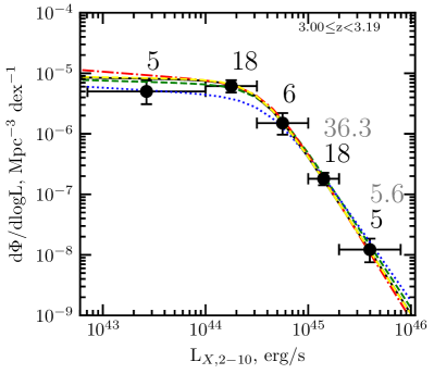
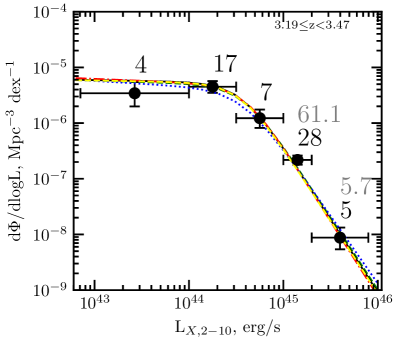
Рис. 6: The differential luminosity function of type 1 quasars as a function of redshift based on the K16 and V14U  subsamples. The points with error bars indicate the binned (nonparametric) estimate of the luminosity function obtained by the $1/V_{\rm max}$ method using the incompleteness correction II. The black font indicates the number of sample objects in the $\Delta\log L$–$\Delta z$ bins under consideration, while the gray font indicates the expected total number of objects corrected for the K16 subsample incompleteness. The black solid, red dash–dotted, green dashed, yellow dashed, and blue dotted lines represent the LADE, LDDE, PDE, ILDE and PLE models, respectively.

5.2 The binned Luminosity Function ($1/V_{\rm max}$)

A nonparametric estimate of the X-ray luminosity function is an estimate of the space density of quasars calculated separately for each of the specified $\Delta\log L$–$\Delta z$ bins from the sample objects falling into these bins. We performed such a calculation by the method described in (Georgakakis , 2015). The space $42.85<\log L<45.9$, $3<z<5.1$ was divided into $\Delta\log L$–$\Delta z$ bins close to those used in Vito (2014). The binning scheme and the number of sources in the corresponding bins are shown in Table LABEL:tab:bindistr and Fig. 1.

Assuming that within each $\Delta\log L$–$\Delta z$ bin (which contains $N$ sources) the luminosity function is constant, i.e., $\phi(L,z,\theta)=C$, we can search for $C$ by the maximum likelihood method using Eqs. (3) and (4), where the constant $C$ in Eq. (4) is the only parameter:

$$\mathcal{L}(C,\Omega,N)=-2\sum^{N}_{i=1}\ln[Cp(d_{i}|L)d\log L]+$$ (6)

$$+2\iint C\Omega(L,z)\frac{dV}{dz}d\log L\,dz.$$

It is easy to show that this function has a minimum at

$$C=\frac{N}{\iint\Omega(L,z)\frac{dV}{dz}d\log L\,dz},$$ (7)

which closely corresponds to the expression from Marshall (1983); Page & Carrera (2000) for calculating the luminosity function by the $1/V_{max}$ method.

The nonparametric estimate of the luminosity function with the incompleteness correction for the K16 subsample obtained in this way is presented in Fig. 6. We see that the analytical luminosity function models pass well through the points obtained by the $1/V_{\rm max}$ method, with the points based on the K16 sample lying on the extension of the law of powerlaw decline in the density of quasars at luminosity $L_{{\rm X},2-10}>10^{45}$ erg/s. It became possible to obtain significant density estimates for distant quasars of such high luminosities only by using the sensitive XMM-Newton X-ray survey with a large area ($\sim 170$ sq. deg at a flux $\sim 4\times 10^{-15}$ erg/s/cm² for the K16  sample).

It should be noted that the nonparametric estimate of the luminosity function disregards the Eddington bias, in contrast to the parametric estimate. Good mutual agreement of both results suggests that the Eddington bias in this case turns out to be insignificant compared to the uncertainties associated with the relatively small K16 sample size and the incompleteness correction.

6 EVOLUTION OF THE SPACE DENSITY OF DISTANT QUASARS

Рис. 7: Evolution of the space density (in comoving coordinates) of distant luminous type 1 quasars. The triangles indicate the density of quasars with $44.5\leq L_{{\rm X},2-10}<45.0$ derived from the V14U subsample; the circles indicate the density of quasars with $45.0\leq\log L_{{\rm X},2-10}<45.3$ and $45.3\leq\log L_{{\rm X},2-10}<45.9$ derived from the K16  subsample for the incompleteness correction II. The hatched regions near the K16  points are the scatter of densities related to the uncertainty in the completeness of this subsample. The lines indicate the luminosity function models for the incompleteness correction II: LADE (black solid line), LDDE (red dash-dotted line), ILDE (yellow dashed line), PDE (green dashed line), and PLE (blue dotted line). The gray dashed line indicates the LADE model from Georgakakis (2015).

Using the above nonparametric estimate of the luminosity function, let us consider the evolution of the space density of high-luminosity quasars with redshift in more detail luminosity bins: $44.5\leq\log L_{{\rm X},2-10}<45.0$ (based on the V14U  subsample) and $45.0\leq\log L_{{\rm X},2-10}<45.3$, $45.3\leq\log L_{{\rm X},2-10}<45.9$ (based on the K16  subsample with the addition of one source from V14U), see Fig. 7. As expected, the K16 survey has allowed reliable estimates of the space density of luminous quasars ($L_{{\rm X},2-10}>10^{45}$ erg/s) at high redshifts to be obtained for the first time. The figure also shows the various luminosity function models discussed in this paper.

It can be seen from Fig. 7 that the comoving density of luminous quasars $45.3\leq\log L_{{\rm X},2-10}<45.9$) changes by no more than a factor of 2 between $z=3$ and $z=5$, while the density of lower-luminosity quasars ($44.5\leq\log L_{{\rm X},2-10}<45.0$) decreases by an order of magnitude (see also Vito et al. 2014; Kalfountzou et al. 2014). In previous papers there has already been evidence for slower evolution of more powerful quasars; now this tendency has become quite obvious owing to the addition of the K16 subsample of luminous quasars. Note that inaccurate knowledge of the K16 sample completeness introduces the main uncertainty in our estimates of the density of luminous quasars at luminosities log $\log L_{{\rm X},2-10}\approx 45$. However, when the luminosity doubles ($\log L_{{\rm X},2-10}\geq 45.3$), the density of sources drops by almost a factor of 10, the sources in the sample become fewer, and the Poissonian errors become large than the scatter of estimates related to incompleteness.

On the whole, the derived redshift dependence of the quasar space density is consistent with the density estimates by Kalfountzou et al. (2014) for unabsorbed quasars at $z>3$. Kalfountzou et al. (2014) made an additional selection (by photometric redshift for objects with apparent magnitude brighter $\mbox{i}^{\prime}<21$) of distant quasars at $z>3$ and for the first time estimated their space density at luminosities $\log L_{{\rm X},2-10}>44.7$ for a survey with an area $\simeq 33$ sq. deg. Quasar candidates selected by $z_{\mbox{\scriptsize phot}}$ constitute half of the sample by (Kalfountzou et al., 2014). We were able to improve significantly the constraints on the density of very luminous ($\log L_{{\rm X},2-10}>45.0$) quasars through an almost tenfold increase in the sky coverage area compared to (Kalfountzou et al., 2014). While in the K16 subsample 90% of quasars have a spectroscopic redshift.

In another recent paper (Georgakakis , 2015) the space density of distant quasars was also estimated from the XMM-XXL survey data. The XMM-XXL sky coverage area and the number of detected quasars at $z>3$ are comparable to the sample by Kalfountzou et al. (2014). Assembling the luminosity function sample Georgakakis (2015) obtained spectroscopic redshifts for most of the X-ray quasar candidates with apparent magnitudes $\mbox{r}^{\prime}<22.5$ (Menzel , 2016). Fig. 7 shows (without errors) the estimates of the space density of luminous quasars obtained from the analytical X-ray luminosity function model from Georgakakis (2015) in the three luminosity bins under consideration. The density estimates in the luminosity range $44.5\leq\log L_{{\rm X},2-10}<45.0$ from the data by Georgakakis (2015) turn out to be slightly lower than those obtained in this paper. The estimates in the mutual luminosity range ($45.0\leq\log L_{{\rm X},2-10}<45.3$) for both samples are in agreement. Possible causes of the discrepancy are discussed in the next section.

7 DISCUSSION

We were able to obtain a large sample (K16) of sources at $z>3$ and luminosities $L_{{\rm X},2-10}>10^{45}$ erg/s, i.e., above the break ($L_{*}\sim 5\times 10^{44}$) in the X-ray luminosity function of quasars, and to determine the slope $\gamma_{2}$ of the bright end of the luminosity function (see Eq. (2)). Since all of the sources from the K16 subsample have luminosities above $L_{*}$, they constrain the slope $\gamma_{2}$. In this case, it should be kept in mind that the luminosities of many of the K16 objects are higher than the presumed break luminosity only by a factor $\gtrsim 2$, i.e., the region in which the slope of the luminosity function changes gradually from $\gamma_{1}$ to $\gamma_{2}$ could be touched.

To reliably determine all parameters of the luminosity function, including $\gamma_{2}$, we supplemented the K16 sample by another sample (V14U) that includes quasars with luminosities $L_{{\rm X},2-10}\lesssim L_{*}$. The V14U ($L_{{\rm X},2-10}\lesssim 10^{45}$ erg/s) and K16 ($L_{{\rm X},2-10}>10^{45}$ erg/s) subsamples complement each other, spanning virtually nonoverlapping luminosity ranges, but, at the same time, having a different completeness.

It follows from Table LABEL:tab:LFA1 that the parameters $A$, $\gamma_{2}$, $L_{*}$ depend on the incompleteness correction more strongly than do the remaining ones. For the listed parameters the bias in their values due to the variations in the incompleteness correction turns out to be larger than or comparable to their statistical errors.

The beginning and the end of the bright slope of the luminosity function is determined, respectively, by the objects with $L>L_{*}$ from V14U  and the luminous objects with $L>2\times 10^{45}$ erg/s from the K16  subsample, whose the incompleteness correction is close to unity. This reduces the uncertainty in the slope $\gamma_{2}$ related to the K16 subsample sources in the luminosity range $10^{45}<L<2\times 10^{45}$ erg/s, for which the uncertainty in the incompleteness correction is great. If $\gamma_{2}$ were determined only with the K16 subsample, then its error and the uncertainties in determining other parameters of the luminosity function would be greater.

The bright end slope of the LDDE luminosity function model and its statistical error are $\gamma_{2}=2.78\pm 0.20$ for incompleteness II. The uncertainty in the quasar detection completeness almost does not affect the slope value.

7.1 Comparison of $\gamma_{2}$ with Previous Estimates

Strictly speaking, our measured slope $\gamma_{2}$ of the X-ray luminosity function of type 1 quasars cannot be compared directly with the results of previous papers (Vito , 2014; Ueda et al., 2014; Georgakakis , 2015), because the parameters of the luminosity function models in them were obtained by taking into account absorbed quasars. However, the statistics of distant high-luminosity quasars ($L_{{\rm X},2-10}>10^{45}$ erg/s) is usually based on large-area X-ray surveys with shallow coverage in the X-ray and optical bands. In such surveys the fraction of the unabsorbed sources found is, as a rule, small (see, e.g., Kalfountzou et al. 2014). In this case, it should be kept in mind that at a small number of X-ray counts it is virtually impossible to distinguish a distant quasar with $N_{\rm H}\simeq 10^{23}$ cm^-2 from a quasar with a lower absorption (Fotopoulou , 2016). Therefore, it can be assumed that the published values of the slope $\gamma_{2}$ are determined mainly by unabsorbed or weakly absorbed sources with $N_{\rm H}\lesssim 10^{23}$ cm^-2, generaly by type 1 AGNs. This allows our estimate of the parameter $\gamma_{2}$ to be approximately compared with the results of other papers.

It is correct to compare the values of $\gamma_{2}$ only within one empirical luminosity function model. Therefore, for comparison with the results of Vito (2014); Georgakakis (2015) we will choose our best LDDE model.

Samples of quasars characterized by a higher optical identification completeness than K16 were used in the papers chosen for our comparison. The sample by Vito (2014) consists of quasars at $z>3$ selected in the 0.5–2 кэВ band and was partially used by us to supplement the K16 catalog by lower luminosity objects. Georgakakis (2015) studied quasars at $z_{\mbox{\scriptsize spec}}>3$ selected in the 0.5-10 keV band in the XMM-XXL survey region with an area of 18 sq. deg. A sample of 59 quasars at $z_{\mbox{\scriptsize spec}}>3$ was obtained through deep spectroscopic support (Menzel , 2016; Georgakakis , 2015) of this region (deeper than on average for SDSS by 2 magnitudes). The XMM-XXL survey was supplemented by data from deep Chandra X-ray surveys (CDFS, CDFN, AEGIS, ECDFS, and C-COSMOS) spanning the luminosity range $10^{43}$–$10^{45}$ erg/s and yielded significant estimates of the density of quasars at luminosities $>10^{45}$ erg/s. Therefore, the results of Georgakakis (2015) turn out to be most interesting for our comparison.

The bright end slope value of the luminosity function $\gamma_{2}=2.78\pm 0.20$ obtained in our paper for the LDDE model and the incompleteness correction II intersects the $1\sigma$ confidence interval of the estimates by Vito (2014) for the LDDE model, $\gamma_{2}=3.71_{-0.84}^{+1.12}$. The $\gamma_{2}$ measurement accuracy improved significantly compared to deep small-area surveys (Vito , 2014). However, there is disagreement with the results from Georgakakis (2015), where a considerably smaller slope was derived for the LDDE model, $\gamma_{2}=2.15\pm 0.24$ (see a comparison of the luminosity functions derived in our paper and Georgakakis (2015) in Fig. 8). The luminosity break $L_{*}=44.31\pm 0.13$ from (Georgakakis , 2015) is also lower than our estimates (see Table LABEL:tab:LFA1).

The estimate of the density of quasars in the range $44.7<\log L_{{\rm X},2-10}<45.3$ from the K16 subsample turns out to be differ than follows from the model by Georgakakis (2015), see Fig. 7. However, it follows from Fig. 8 that the difference between the models is not that significant and they agree between themselves, within the statistical error limits. A discrepancy of the density at the highest luminosity range where K16 has objects is interesting for further research.

Рис. 8: The differential luminosity function in two broad redshift intervals. The points with error bars indicate the binned luminosity function obtained by $1/V_{\rm max}$ method using the incompletenes correction II. The black font indicates the number of sample objects in the $\Delta\log L$–$\Delta z$ bins under consideration, while the gray font indicates the expected total number of objects corrected for the K16  subsamble incompleteness II. The black solid line represents the LDDE model computed for the incompleteness correction II. The dashed line indicates the LDDE model from Georgakakis (2015).

The difference in the estimates of $\gamma_{2}$ and $L_{*}$ under discussion can be caused by the following factors. First, at luminosities $L_{{\rm X},2-10}\lesssim 5\times 10^{44}$ erg/s sources from deep surveys appear in the sample by Georgakakis (2015), and their contribution changes significantly the density distribution with respect to unabsorbed quasars. That is why the points belonging the V14U subsample in Fig. 8 lie well below the model by Georgakakis (2015).

Second, the area of the deep surveys used in Georgakakis (2015) is half the area of the deep surveys from Vito (2014) used in our paper. Consequently, in the sample by Vito (2014) there are more objects with luminosities near the break luminosity $L_{*}\simeq 5\times 10^{44}$ erg/s (Vito , 2014) than in the deep surveys of the sample by Georgakakis (2015), and, therefore, the sample by Vito (2014) allows $L_{*}$ to be determined more accurately.

Third, in contrast to our paper and Vito (2014), in which a certain value of photometric redshifts $z_{\mbox{\scriptsize phot}}$ were assigned to the objects, a probabilistic approach was used in Georgakakis (2015): the probability density distribution of possible $z_{\mbox{\scriptsize phot}}$ was сonsidered for each object from the deep surveys. Georgakakis (2015) showed that using fixed $z_{\mbox{\scriptsize phot}}$ in analyzing the data of deep surveys, such as COSMOS, could lead to an overestimate (by a factor of 1.8–3) of the density of quasars at luminosities $\lesssim 5\times 10^{44}$ erg/s. Therefore, some of the photometric candidates from the V14U subsample may turn out to be quasars at lower $z$ and the slope $\gamma_{2}$ will then be shallower. The slope $\gamma_{2}$ can be overestimated if type 2 quasars, without broad lines in the optical spectrum (see Fig. 5), are present among the photometric quasar candidates with $N_{\rm H}\leqslant 10^{23}$ cm^-2 from the V14U subsample. In the range $44.5<\log L_{{\rm X},2-10}<45.0$, which defines the beginning of the slope $\gamma_{2}$, the fraction of photometric candidates in the V14U subsample is about 20%. Therefore, if there are absorbed quasars or quasars $z<3$ among the $z_{\mbox{\scriptsize phot}}$ candidates, then this will not affect strongly the estimate of the slope $\gamma_{2}$.

Fourth, the spectroscopic sample by Menzel (2016) used in Georgakakis (2015) may be subjected to optical identification incompleteness at 0.5–2 keV X-ray fluxes $\lesssim 5\times 10^{-15}$ erg/s/cm² corresponding to luminosities$\sim 5\times 10^{44}$ erg/s for quasars at $z>3$. In that case, the measurements will show a shallower slope $\gamma_{2}$ than the actual one.

All of the listed factors can lead to a mismatch between the values of $L_{*}$ and $\gamma_{2}$ that were obtained in this paper and Georgakakis (2015).

In Fig. 9 the values of the slope $\gamma_{2}$ derived in our paper are compared with the results of Vito (2014); Georgakakis (2015). It can be clearly seen that using the K16 objects that we selected based on the data of a large-area X-ray survey, we were able to constrain the slope of the bright end of the X-ray luminosity function for distant quasars much better than can be done based only on the data of small-area deep surveys (Vito , 2014). The same figure shows the values of $\gamma_{2}$ from Ueda et al. (2014); Aird et al. (2015); Ranalli (2016), where the luminosity function models were constructed based on samples of quasars spanning a wide range of luminosities and redshifts. In these papers the quasars at $z>3$ account for only a few percent of the total size of the samples, which consist of absorbed and unabsorbed quasars; in addition, more complex luminosity function models dependent on a larger number of evolution parameters were used. Therefore, the values of $\gamma_{2}$ obtained in these papers characterize the distribution of more nearby quasars.

Рис. 9: Comparison of the bright end slope ($\gamma_{2}$) obtained in this paper (K18) with the values reported before, for the LDDE luminosity function model. The black circle with error bars indicates the slope value and its statistical uncertainty $\gamma_{2}=2.78\pm 0.20$ for the LDDE model, for incompleteness correction II. The gray error bars show the range of $\gamma_{2}$ values for incompleteness corrections I and III, taking into account statistical errors. The green triangles denote the LDDE $\gamma_{2}$ values and the corresponding statistical errors obtained for quasar samples at $z>3$: V14 (Vito , 2014); G15 (Georgakakis , 2015). The blue squares show the LDDE $\gamma_{2}$ estimates obtained for large quasar samples spanning a wide range of luminosities and redshifts, in which high-redshift objects at $z>3$ constitute just a few percent of the total sample: U14 (Ueda et al., 2014); A15 (Aird et al., 2015) — a soft-band sample; R16 (Ranalli , 2016).

8 CONCLUSIONS

In this paper we obtained estimates of the X-ray luminosity function for type 1 quasars for a sample of 101 sources with luminosities $L_{X,2-10}\geqslant 10^{45}$ erg/s from our catalog (Khorunzhev , 2016). The LDDE, LADE, ILDE, and PDE luminosity function models describe equally well the density distribution of unabsorbed quasars. The constraints on the bright end slope of the X-ray luminosity luminosity function ($\gamma_{2}=2.78\pm 0.20$ for the LDDE model) were improved.

The values of $\gamma_{2}$ and other model parameters depend on the choice of a quasar incompleteness correction for the K16 catalog. As the correction increases, the slope $\gamma_{2}$ becomes steeper and the break luminosity grows.

The necessity of taking into account this correction stems from the fact that only for sources with $\mbox{z}^{\prime}<20.5$ we can make photometric redshift estimates using the entire set of SDSS filters, thus improving the reliability and accuracy of $z_{\mbox{\scriptsize phot}}$. In this case, some of the X-ray luminous quasars at $z>3$ turn out to be fainter than the chosen optical threshold and will be missed in the selection.

Most of the K16  sources selected by $z_{\mbox{\scriptsize phot}}$ are spectroscopically confirmed SDSS quasars. The sample of distant X-ray quasars at luminosities $L_{X,2-10}>10^{45}$ erg/s can be expanded by 20% by the method of searching for new candidates for distant quasars described in Khorunzhev (2016). These candidates are confirmed by the spectroscopic observations performed at the following telescopes: АZT-33IK (Kamus , 2002) with the ADAM low-resolution spectrograph (Afanasiev , 2016; Burenin et al., 2016) and BTA with the SCORPIO-I (Afanasiev & Moiseev, 2005) and SCORPIO-II (Afanasiev & A. Moiseev, 2011; Afanasiev & Amirkhanyan, 2012) spectrographs (see Khorunzhev (2017a, b); G. Khorunzhev (2019)).

The produced X-ray sample of luminous quasars at $z>3$ is one of the most extensive in sky coverage area and number of luminous sources. It can be used as a reference one to estimate the completeness and purity of the methods for the selection of distant quasars and to test the algorithms for optical identifications of X-ray sources from the planned SRG all-sky survey (Pavlinsky , 2011; Merloni, 2014).

An X-ray quasar at $z=3$ with a 0.5–2 keV flux $\simeq 10^{-14}$ erg/s/cm² has a 2–10 keV luminosity $L_{{\rm X},2-10}\simeq 10^{45}$ erg/s. This means that $z_{\mbox{\scriptsize phot}}$ in SDSS fields can be obtained for $\gtrsim 50$% of the X-ray quasars at $z\sim 3$ found in the SRG/eROSITA survey (Merloni, 2014) with fluxes $\gtrsim 10^{-14}$ erg/s/cm², which corresponds to the average sensitivity of a four-year survey over the sky. It will be possible to refine the break luminosity ($L_{*}\simeq 4\times 10^{44}$ erg/s) using the data of deep SRG survey fields near the poles of the ecliptic, where a sensitivity $F_{{\rm X},0.5-2}\simeq 2\times 10^{-15}$ erg/s/cm² will be achieved.

We are planning to expand the existing sample of distant X-ray quasars through new X-ray (XMM-Newton) and optical (SDSS, Pan-STARRS) data, to improve the selection methods (see, e.g., Meshcheryakov et al. 2015, and to continue the program of their spectroscopic identification with the AZT-33IK and BTA telescopes.

9 ACKNOWLEDGMENTS

This study was supported by RSF (project No. 14-22-00271). The observations at the 6-m BTA telescopes were financially supported by the Ministry of Education and Science of the Russian Federation (contract no. 14.619.21.0004, project identifier RFMEFI61914X0004). The AZT-33IK observations were done by using the equipment of Center for Common Use "Angara" http://ckp-rf.ru/ckp/3056/. The working capacity of AZT-33IK equipment was supported by funding of Basic Research program II.16. We would like to thank V. Astakhov for translation of the paper in English.

Таблица 1: The sample of sources from the K16 catalog with $L_{{\rm X},2-10}>10^{45}$ erg/s

N	No	Name	OBJID	RA	DEC	$z$	$z_{\rm ref}$	$F_{{\rm X},0.5-2}$	$L_{{\rm X},2-10}$
1	5	J000443.6$-$084036	1237680240914071885	1.1820	-8.6761	3.85		0.94	45.21
2	8	J000618.1$-$084410	1237672793424200167	1.5758	-8.7359	3.323	1	0.87	45.03
3	27	J002706.9+261559	1237680275262538220	6.7800	26.2667	3.29		0.94	45.06
4	30	J003000.5+044040	1237678661427266242	7.5034	4.6784	3.091	1411	1.00	45.02
5	35	J004054.6$-$091527	1237652948530037577	10.2277	-9.2575	5.002	1	1.11	45.53
6	42	J004505.3$-$014048	1237678881562427510	11.2721	-1.6800	3.282	1	1.00	45.08
7	45	J004800.9+315354	1237680310696804736	12.0039	31.8986	3.18		1.40	45.19
8	50	J005952.7+314403	1237680310697919062	14.9693	31.7343	3.30		1.84	45.35
9	87	J020229.4$-$042703	1237679323396309357	30.6225	-4.4509	3.23		2.11	45.39
10	89	J020316.4$-$074831	1237679338956325563	30.8182	-7.8090	3.296	1	1.24	45.18
11	107	J021126.4$-$054022	1237679321786614354	32.8598	-5.6731	3.399	1	0.99	45.11
12	115	J021401.9$-$003941	1237663783138296681	33.5082	-0.6617	4.17		0.63	45.11
13	133	J022037.4$-$061037	1237679340568903780	35.1561	-6.1769	3.03		1.01	45.01
14	141	J022112.5$-$034251	1237679323935212347	35.3026	-3.7145	5.011	1	0.62	45.28
15	144	J022307.9$-$030840	1237679255745790580	35.7832	-3.1445	3.675	1	0.77	45.07
16	153	J022320.7$-$031823	1237678887988429287	35.8363	-3.3068	3.865	1	2.19	45.58
17	163	J022826.5$-$085501	1237652900227252760	37.1099	-8.9175	3.24		1.17	45.13
18	167	J022906.0$-$051428	1237679253062091149	37.2752	-5.2414	3.173	1	1.93	45.33
19	180	J023441.1$-$040711	1237679323399782556	38.6713	-4.1197	3.334	1	0.95	45.07
20	192	J030449.8$-$000814	1237666300553789504	46.2077	-0.1371	3.287	1	4.81	45.76
21	245	J084617.8+190342	1237667211581522773	131.5738	19.0620	3.47	2	0.99	45.13
22	257	J085822.2+564533	1237660936091796090	134.5925	56.7590	3.021	1	1.34	45.12
23	282	J091959.5+370550	1237660634915406290	139.9984	37.0974	3.379	1	0.80	45.01
24	286	J092143.5+063644	1237658425155977396	140.4313	6.6121	3.718	1	1.00	45.20
25	287	J092325.3+453223	1237657401346424982	140.8552	45.5395	3.452	1	1.49	45.30
26	292	J093404.6+472434	1237657590848618536	143.5195	47.4095	3.086	1	1.74	45.26
27	293	J093451.6+353744	1237661384382480820	143.7148	35.6290	3.363	1	0.96	45.08
28	296	J093709.6+495147	1237657770707976723	144.2908	49.8642	3.641	1411	3.00	45.66
29	318	J095937.0+131212	1237664106852384915	149.9046	13.2043	4.064	1411	1.88	45.56
30	338	J101515.2+085456	1237660584444953274	153.8140	8.9159	3.235	1	1.46	45.23
31	347	J102107.5+220922	1237667538009588107	155.2816	22.1560	4.262	1	1.74	45.57
32	370	J103428.8+393343	1237661383314178468	158.6203	39.5621	4.334	1411	1.38	45.49
33	382	J104612.9+584719	1237655109446467756	161.5541	58.7886	3.054	1	1.53	45.19
34	385	J104909.8+373758	1237664668437774491	162.2909	37.6331	3.005	1	6.95	45.83
35	396	J105049.2+354517	1237664819280347214	162.7057	35.7557	3.326	1411	0.88	45.04
36	398	J105123.0+354535	1237664819280412861	162.8460	35.7595	4.921	1	1.73	45.71
37	411	J110458.2+250421	1237667551956369534	166.2428	25.0728	3.522	1	1.80	45.40
38	430	J111900.0+152707	1237661070867431568	169.7508	15.4520	3.138	1	1.12	45.08
39	431	J112020.9+432545	1237661850390954212	170.0874	43.4292	3.555	1	0.88	45.10
40	447	J114323.7+193447	1237667915416600770	175.8488	19.5800	3.348	1	1.19	45.17
41	449	J114447.7+370434	1237664818748260677	176.1986	37.0763	4.010	1	1.77	45.52
42	453	J114816.0+525900	1237657857682899337	177.0670	52.9831	3.173	1	6.74	45.87
43	459	J115839.8+262510	1237667429035869276	179.6659	26.4197	3.428	1	0.94	45.09
44	460	J115933.3+553632	1237657591395844307	179.8888	55.6091	3.981	1	0.58	45.03
45	463	J120125.5+064621	1237671140947592014	180.3563	6.7729	3.323	1	1.24	45.18
46	476	J120949.7+453400	1237661873476534381	182.4573	45.5668	3.609	1	2.72	45.61
47	510	J122602.0+132114	1237661813886091391	186.5088	13.3540	3.530	1	1.95	45.44
48	523	J123136.8+131544	1237661950792696231	187.9030	13.2617	3.48	2	0.99	45.13
49	524	J123005.9+142957	1237664289929494661	187.5244	14.4989	3.275	1	1.56	45.27
50	525	J123011.9+102237	1237662238004412598	187.5500	10.3771	3.569	1	1.00	45.16
51	529	J123157.3+000933	1237648704579108962	187.9891	0.1590	3.226	1	0.95	45.04
52	538	J123503.1$-$000331	1237648721234559206	188.7627	-0.0588	4.701	1	2.27	45.78
53	553	J124210.7+024049	1237671765324595744	190.5448	2.6804	3.175	1	3.12	45.54
54	569	J125736.2+242040	1237667911133888887	194.4003	24.3444	3.681	1	0.92	45.15
55	579	J130616.9+264335	1237667322724680051	196.5703	26.7264	3.208	1	1.21	45.14
56	580	J130811.9+292512	1237665428627456150	197.0497	29.4202	3.035	1	1.11	45.04
57	592	J131236.2+231629	1237667910061654088	198.1511	23.2751	3.684	1	0.65	45.00
58	618	J133200.0+503613	1237662301357736036	202.9998	50.6037	3.84	2	0.78	45.12
59	619	J133223.2+503430	1237662301357736105	203.0969	50.5754	3.832	1	0.94	45.20
60	627	J134135.6$-$001321	1237648704049840848	205.3980	-0.2230	3.919	1	0.67	45.07
61	653	J140146.5+024433	1237651754560520506	210.4439	2.7430	4.424	1	1.06	45.39
62	675	J142926.4+011951	1237651752952923130	217.3601	1.3316	4.840	1297	0.51	45.17
63	693	J145753.0$-$011358	1237648702984422397	224.4710	-1.2330	3.503	1	1.33	45.26
64	704	J151147.1+071406	1237662237485039775	227.9465	7.2350	3.481	1	2.58	45.55
65	710	J151534.3$-$000000	1237648721252122996	228.8933	-0.0002	3.04	2	1.38	45.14
66	731	J154905.8+352020	1237662503219364016	237.2744	35.3390	3.038	1	2.60	45.42
67	745	J160528.3+272852	1237662307273999256	241.3675	27.4818	4.023	1	0.77	45.16
68	755	J162114.9$-$021130	1237668651464918353	245.3125	-2.1918	4.34	2	0.67	45.17
69	762	J163207.9+571108	1237668505439503219	248.0339	57.1863	3.40	2	1.04	45.13
70	766	J163459.2+332510	1237661386008298072	248.7476	33.4194	3.237	1	1.36	45.20
71	782	J171337.2+585306	1237651225708921950	258.4049	58.8853	4.37	2	0.76	45.24
72	796	J203958.0$-$004337	1237656567574104067	309.9923	-0.7273	4.63		0.44	45.06
73	816	J212959.5+051005	1237669762254439608	322.4981	5.1683	3.02		1.01	45.00
74	826	J215139.1+021628	1237678597539561948	327.9136	2.2740	3.256	1	0.97	45.06
75	837	J221753.2$-$003257	1237663542611083691	334.4730	-0.5486	3.106	1411	1.69	45.25
76	840	J222008.9$-$002343	1237663478722658939	335.0375	-0.3955	3.344	1	0.89	45.05
77	856	J230252.1+085522	1237679034548486973	345.7172	8.9225	3.750	1	0.64	45.02
78	859	J231619.4+254552	1237666184031633742	349.0811	25.7647	3.207	1	1.01	45.06
79	863	J231839.7+002032	1237666408437907970	349.6655	0.3421	3.23		1.11	45.11
80	866	J232137.4+283025	1237680331636474144	350.4056	28.5072	3.062	1	1.67	45.23
81	871	J232346.0+165228	1237678601301459610	350.9415	16.8744	3.602	1	1.22	45.25
82	872	J232419.4+165620	1237678601301524724	351.0810	16.9389	3.323	1	1.50	45.27
83	890	J234214.1+303606	1237666183498039666	355.5590	30.6017	3.37	2	0.80	45.01
84	897	J235054.6+200939	1237680246813491428	357.7276	20.1607	3.162	1	1.00	45.04
85	898	J235201.3+200901	1237680246813556916	358.0054	20.1507	3.079	1	1.16	45.08
86	901	J235435.5$-$101513	1237652900210671714	358.6483	-10.2537	3.120	1	1.16	45.09
87	*2	J002654.9+171944	1237678601308078496	6.7290	17.3290	3.095	1	1.12	45.07
88	*6	J020231.1$-$042246	1237679323396309664	30.6298	-4.3797	4.270	1	1.28	45.44
89	*9	J021338.6$-$051615	1237679253060387565	33.4110	-5.2711	4.544	1	0.93	45.36
90	*13	J022251.7$-$050713	1237679322324795732	35.7157	-5.1202	3.860	1758	0.88	45.18
91	*17	J023226.0$-$053729	1237679341107085527	38.1089	-5.6249	4.564	1	0.53	45.12
92	*24	J093521.2+612339	1237651272966275457	143.8391	61.3942	4.042	1	0.69	45.12
93	*25	J094013.9+344628	1237661382772130308	145.0579	34.7747	3.355	1	2.30	45.46
94	*30	J100655.8+050325	1237658297920454886	151.7325	5.0569	3.086	1	1.45	45.18
95	*33	J104808.3+583718	1237658304353272305	162.0354	58.6210	3.285	1	1.14	45.13
96	*43	J124405.1+125757	1237661817633374639	191.0211	12.9658	3.100	611	1.10	45.06
97	*51	J140149.8+024835	1237651754560520571	210.4579	2.8102	3.830	643	0.98	45.22
98	*54	J150603.5+012757	1237651753493791548	226.5146	1.4662	3.852	1	0.79	45.13
99	*56	J164829.7+350159	1237659326568858151	252.1238	35.0330	4.075	1347	3.53	45.84
100	*57	J171456.2+593700	1237651226245530116	258.7344	59.6169	4.028	1406	1.20	45.36
101	*61	J220845.5+020252	1237678597004591287	332.1895	2.0479	3.405	646	1.00	45.12
Notes: N is the source number, No is the ordinal source number in the catalog (K16) Khorunzhev (2016), the asterisk <<*>> marks sources have being taken from the additional table of quasars with $z_{\mbox{\scriptsize spec}}>3$ that did not enter into the catalog of candidates in the paper Khorunzhev (2016), Name — is the name in the 3XMM-DR4 (3XMMJ…) catalog, OBJID — is the identifier in the photometric SDSS–DR12 catalog, RA and DEC are the right ascension and declination (SDSS–DR12) in degrees, $z$ is the redshift of the source, $z_{\rm ref}$ is a reference to the redshift: the empty field is the photometric redshift (Khorunzhev , 2016), 1 is the SDSS–DR12 spectroscopy (Alam , 2015), 2 is the АZT-33IK и BTA spectroscopy (Khorunzhev , 2017a, b; G. Khorunzhev , 2019); the remaining redshifts were taken from the catalog Flesch 2015 (the reference numbers correspond to Flesch (2015): 611 — Flesch (2015), 643 — (Gandhi , 2002), 646 — Garilli (2014), 1297 — Monier  (2002), 1347 — Newman  (2013), 1406 — Papovich (2006), 1411 — Paris (2017), 1758 — Stalin  (2010)), $F_{{\rm X},0.5-2}$ is the 0.5–2 keV X-ray flux $\times 10^{-14}$ erg/s/cm2, $L_{{\rm X},2-10}$ is the decimal logarithm of the source’s 2–10 keV luminosity (erg/s) in its rest frame.

Таблица 1: *

Таблица 2: Parameters of the X-ray luminosity function models for the V14U and K16  subsamples.

Модель	$\log A$	$\log L_{*}$	$\gamma_{1}$	$\gamma_{2}$	$p_{\rm lum}$	$p_{\rm den}$	$\beta$	$\Delta AIC$	$\Delta BIC$
PDE	-5.15${}^{+0.11(-0.11)}_{-0.11(0.08)}$	44.58${}^{+0.07(0.15)}_{-0.08(-0.09)}$	0.05${}^{+0.15(0.09)}_{-0.17(-0.07)}$	2.59${}^{+0.18(-0.03)}_{-0.17(0.00)}$	—	-4.83${}^{+0.68(0.20)}_{-0.70(-0.27)}$	—	2.3	0.0
ILDE	-5.04${}^{+0.12(-0.11)}_{-0.13(0.06)}$	44.51${}^{+0.08(0.14)}_{-0.09(-0.08)}$	0.03${}^{+0.16(0.12)}_{-0.18(-0.08)}$	2.62${}^{+0.18(0.03)}_{-0.17(-0.01)}$	1.35${}^{+0.70(0.58)}_{-0.70(-0.31)}$	-7.04${}^{+1.34(-0.35)}_{-1.36(0.11)}$	—	0.6	1.7
LADE	-5.06${}^{+0.12(-0.11)}_{-0.12(0.06)}$	44.51${}^{+0.08(0.14)}_{-0.09(-0.08)}$	0.03${}^{+0.16(0.12)}_{-0.18(-0.08)}$	2.61${}^{+0.18(0.03)}_{-0.17(-0.01)}$	1.38${}^{+0.71(0.56)}_{-0.70(-0.30)}$	-0.65${}^{+0.12(-0.03)}_{-0.12(0.01)}$	—	0.3	1.3
LDDE	-5.13${}^{+0.12(-0.13)}_{-0.12(0.08)}$	44.59${}^{+0.07(0.14)}_{-0.07(-0.09)}$	0.16${}^{+0.16(0.11)}_{-0.18(-0.09)}$	2.78${}^{+0.20(0.00)}_{-0.19(-0.04)}$	—	-6.95${}^{+1.27(-0.24)}_{-1.33(0.08)}$	2.64${}^{+1.31(0.57)}_{-1.28(-0.45)}$	0.0	1.0
PLE	-5.40${}^{+0.12(-0.10)}_{-0.12(0.07)}$	44.64${}^{+0.08(0.14)}_{-0.09(-0.09)}$	0.10${}^{+0.15(0.08)}_{-0.17(-0.06)}$	2.43${}^{+0.17(-0.08)}_{-0.16(0.02)}$	-2.10${}^{+0.39(0.01)}_{-0.41(-0.12)}$	—	—	24.6	22.4
Notes: LDDE, ILDE, LADE, PDE, PLE are the models under consideration, $\log A$ is the decimal logarithm of the normalization factor (Мpc-3), $\log L_{*}$ is the decimal logarithm of the break luminosity (erg/s), $\gamma_{1}$ and $\gamma_{2}$ are the exponents for the faint and bright slopes of the luminosity function, $p_{\rm lum}$ is the luminosity evolution parameter, $p_{\rm den}$ is the density evolution parameter, $\beta$ is an additional parameter that accounts for the luminosity dependency of the LDDE model, $\Delta{AIC}$ and $\Delta{BIC}$ are the differences of the AIC and BIC information criteria for a given model and the model with the lowest AIC (LDDE) и BIC (PDE) values . The parameters and their statistical errors (1$\sigma$) are given for the incompleteness correction II. The shift of the parameters for the incompleteness corrections I and III relative to the incompleteness correction II is given in parentheses at the bottom and the top, respectively.

Таблица 2: *

Таблица 3: The number of sources in $\Delta\log L$–$\Delta z$ bins

$\Delta\log L$/$\Delta z$	3.00–3.19	3.19–3.47	3.47–3.90	3.90–4.30	4.30–5.10
42.9-44.0	5/-	4/-	4/-	1/-	-/-
44.0-44.5	18/-	17/-	15/-	5/-	2/-
44.5-45.0	6/-	7/-	11/-	5/-	3/-
45.0-45.3	-/18	1/27	-/17	-/5	-/6
45.3-45.9	-/5	-/5	-/6	-/6	-/6
Notes: The rows in the table show the binning by logarithm of the X-ray luminosity $L_{{\rm X},2-10}$. The columns show the binning by redshift $z$. In the cells of the table the number of objects in a given bin from the V14U  and K16 samples is specified on the left and the right, respectively.

Таблица 3: *