Counting Feynman diagrams via many-body relations

Abstract

We present an iterative algorithm to count Feynman diagrams via many-body relations. The algorithm allows us to count the number of diagrams of the exact solution for the general fermionic many-body problem at each order in the interaction. Further, we apply it to different parquet-type approximations and consider spin-resolved diagrams in the Hubbard model. Low-order results and asymptotics are explicitly discussed for various vertex functions and different two-particle channels. The algorithm can easily be implemented and generalized to many-body relations of different forms and levels of approximation.

I Introduction

In the study of many-particle systems, Feynman diagrams are a ubiquitous, powerful tool to perform and organize perturbation series as well as partial resummations thereof. To gain intuition about the strength of a diagrammatic resummation or to compare different variants of resummation, it can be useful to count the number of diagrams involved, ideally for several kinds of vertex functions. Moreover, the factorial growth in the number of diagrams with the interaction order is often linked with the nonconvergent, asymptotic nature of (bare) perturbation series Negele and Orland (1998). The asymptotic number of diagrams generated by approximate solutions is therefore of particular interest.

In this paper, we present an algorithm to count the number of Feynman diagrams inherent in many-body integral equations. Its iterative structure allows us to numerically access arbitrarily large interaction orders and to gain analytical insights about the asymptotic behavior. In Sec. II, we recapitulate typical many-body relations as a basis for the algorithm. The algorithm is explained in Sec. III, where some general parts of the discussion follow Ref. Kugler and von Delft, 2018a quite closely; some of the ideas have also been formulated by Smith Smith (1992). In Sec. IV, we use the algorithm to count the exact number of bare and skeleton diagrams of the general many-body problem for various vertex functions and to discuss their asymptotics. Subsequently, we consider parquet-type approximations as examples for approximate solutions, and we focus on the Hubbard model to discuss spin-resolved diagrams. Finally, we present our conclusions in Sec. V.

II Many-body relations

A general theory of interacting fermions is defined by the action

$$S =-\sum_{x^{\prime},x}\bar{c}_{x^{\prime}}\big{(}G_{0}^{-1}\big{)}_{x^{\prime},x}c_{x}-\tfrac{1}{4}\!\!\!\!\sum_{x^{\prime},x,y^{\prime},y}\!\!\!\!\Gamma^{(4)}_{0;x^{\prime},y^{\prime};x,y}\bar{c}_{x^{\prime}}\bar{c}_{y^{\prime}}c_{y}c_{x},$$ (1)

where $G_{0}$ is the bare propagator, $\Gamma^{(4)}_{0}$ the bare four-point vertex, which is antisymmetric in its first and last two arguments, and $x$ denotes all quantum numbers of the Grassmann field $c_{x}$. If we choose, e.g., Matsubara frequency, momentum, and spin, with $x=(i\omega,\bm{k},\sigma)=(k,\sigma)$, and consider a translationally invariant system with interaction $U_{|\bm{k}|}$, the bare quantities read

$$G_{0;x^{\prime},x} \overset{\textrm{e.g.}}{=}G_{0;k,\sigma}\delta_{k^{\prime},k^{\phantom{\prime}}}\delta_{\sigma^{\prime},\sigma^{\phantom{\prime}}},$$ (2a)

$$-\Gamma^{(4)}_{0;x_{1}^{\prime},x_{2}^{\prime};x_{1}^{\phantom{\prime}},x_{2}^{\phantom{\prime}}} \overset{\textrm{e.g.}}{=}(U_{|\bm{k}_{1}^{\prime}-\bm{k}_{1}^{\phantom{\prime}}|}\delta_{\sigma_{1}^{\prime},\sigma_{1}^{\phantom{\prime}}}\delta_{\sigma_{2}^{\prime},\sigma_{2}^{\phantom{\prime}}}$$

$$\,\ -U_{|\bm{k}_{1}^{\prime}-\bm{k}_{2}^{\phantom{\prime}}|}\delta_{\sigma_{1}^{\prime},\sigma_{2}^{\phantom{\prime}}}\delta_{\sigma_{2}^{\prime},\sigma_{1}^{\phantom{\prime}}})\,\delta_{k_{1}^{\prime}+k_{2}^{\prime},k_{1}^{\phantom{\prime}}+k_{2}^{\phantom{\prime}}}.$$ (2b)

Interested in one- and two-particle correlations, the many-body theory is usually focused on the full propagator $G$ with self-energy $\Sigma$ and the full one-particle-irreducible (1PI) four-point vertex $\Gamma^{(4)}$, which can be decomposed into two-particle-irreducible vertices $I_{r}$ in different two-particle channels $r\in\{a,p,t\}$ (see below). The quantities $G$, $\Sigma$, $\Gamma^{(4)}$ are related by the exact and closed set of equations Hedin (1965); Bickers (2004); Held et al. (2011); Kugler and von Delft

$$G =G_{0}+G_{0}\cdot\Sigma\cdot G,$$ (3a)

$$\Sigma =-\Gamma^{(4)}_{0}\circ G-\tfrac{1}{2}\Gamma^{(4)}_{0}\circ G\circ G\circ G\circ\Gamma^{(4)},$$ (3b)

$$\Gamma^{(4)} =I_{t}-I_{t}\circ G\circ G\circ\Gamma^{(4)},\quad I_{t}=-\frac{\delta\Sigma}{\delta G},$$ (3c)

where $\cdot$ represents a matrix product and $\circ$ a suitable contraction of indices . The first equation is the well-known Dyson equation, the second one the Schwinger-Dyson equation (SDE, or equation of motion) for the self-energy, and the last one a Bethe-Salpeter equation (BSE), where the irreducible vertex $I_{t}$ is obtained by a functional derivative of $\Sigma$ w.r.t. $G$. These equations together with further equations discussed below are illustrated in Fig. 1.

Figure 1: Graphical representation of many-body relations, where solid lines represent dressed propagators $G$ and dots represent bare four-point vertices $\Gamma_{0}^{(4)}$. (a) Schwinger-Dyson equation (3b) for the self-energy. (b) To perform the functional derivative $\delta\Sigma/\delta G$ in Eq. (3c), one sums all copies of diagrams where one $G$ line is removed. Conversely, the self-energy differentiated w.r.t. a scalar parameter (see main text), $\dot{\Sigma}$, is obtained by contracting [cf. Eq. (5a)] the vertex $I_{t}$ with $\dot{G}$ (line with double dash) or [cf. Eq. (5b)] the full vertex $\Gamma^{(4)}$ with the singled-scale propagator $S$ [cf. Eq. (4), line with one dash]. (c) $\Gamma^{(4)}$ deduced from the Bethe-Salpeter equation (BSE) in the transverse channel (3c). (d)–(e) BSEs (7) for the reducible vertices in (d) the antiparallel channel and (e) the parallel channel. (f) Dyson equation (3a) involving the bare propagator $G_{0}$ (gray line). Note that the relations (a)–(c) suffice to generate all skeleton diagrams for the self-energy and the vertex (with all signs and prefactors written explicitly). Relations (c)–(e) together with Eq. (6) enable the parquet decomposition of the four-point vertex. Finally, the Dyson equation (f) makes the connection between bare and skeleton diagrams.

The relation between $I_{t}$ and $\Sigma$ is closely related Kugler and von Delft to an exact flow equation of the functional renormalization group (fRG) framework Metzner et al. (2012); Kopietz et al. (2010). There, the theory evolves under the RG flow by variation of a scale parameter $\Lambda$, introduced in the bare propagator. Consequently, all vertex functions develop a scale dependence (which is suppressed in the notation), and an important role is attached to the so-called single-scale propagator

$$S=\dot{G}-G\cdot\dot{\Sigma}\cdot G=(\mathbbm{1}+G\cdot\Sigma)\cdot\dot{G}_{0}\cdot(\Sigma\cdot G+\mathbbm{1}),$$ (4)

where $\dot{G}=\partial_{\Lambda}G$, etc. If the variation of $G$ in Eq. (3c) is realized by varying $\Lambda$, one obtains by inserting Eq. (4)

$$\dot{\Sigma} =-I_{t}\circ\dot{G}=-I_{t}\circ(S+G\cdot\dot{\Sigma}\cdot G)$$ (5a)

$$=-(I_{t}-I_{t}\circ G\circ G\circ I_{t}+\dots)S=-\Gamma^{(4)}\circ S.$$ (5b)

The iterative insertion of $\dot{\Sigma}$ on the r.h.s. yields a ladder construction in the $t$ channel that produces the full vertex $\Gamma^{(4)}$ from $I_{t}$ [cf. Eq. (3c)] and results in the well-known flow equation of the self-energy Metzner et al. (2012); Kopietz et al. (2010).

Finally, the relation between the full and the two-particle-irreducible vertices is made precise by the parquet equation Bickers (2004); Roulet et al. (1969)

$$\textstyle\Gamma^{(4)}=R+\sum_{r}\gamma_{r},\quad I_{r}=R+\sum_{r^{\prime}\neq r}\gamma_{r^{\prime}}.$$ (6)

Here, $R$ is the totally irreducible vertex, whereas the vertices $\gamma_{r}$ with $r\in\{a,p,t\}$ are reducible by cutting two antiparallel lines, two parallel lines, or two transverse (antiparallel) lines, respectively . They are obtained from the irreducible ones via the BSEs [cf. Eq. (3c) and Figs. 1(c)–1(e)]

$$\gamma_{r} =\sigma_{r}\,I_{r}\circ G\circ G\circ\Gamma^{(4)},\ \ \sigma_{a}=1=-\sigma_{t},\ \sigma_{p}=\tfrac{1}{2}.$$ (7)

The relative minus sign in the $a$ and $t$ channel stems from the fact that $\gamma_{a}$ and $\gamma_{t}$ are related by exchange of fermionic legs. Following the conventions of Bickers Bickers (2004), the factor of $1/2$ used in the $p$ channel and in Eq. (3b) ensures that, when summing over all internal indices, one does not overcount the effect of the two indistinguishable (parallel) lines connected to the antisymmetric vertices.

III Counting of diagrams

A key aspect in the technique of many-body perturbation theory is that all quantities have (under certain conventions) a unique representation as a sum of diagrams, which can be obtained by following the so-called Feynman rules. In order to count the number of diagrams via many-body integral equations, we express all quantities as sums of diagrams (i.e., we expand in the interaction) and collect all combinations that lead to the same order in the interaction. These combinations of different numbers of diagrams yield the number of diagrams for the resulting object. In fact, the multiplicative structure in the interaction translates into discrete convolutions of the individual numbers of diagrams. Since the interaction vertices start at least at first order in the interaction, the resulting equations can be solved iteratively.

As a first example, we count the number of diagrams in the full propagator $G$ at order $n$ in the interaction, $\mathcal{N}_{G}(n)$, given the number of diagrams in the self-energy, $\mathcal{N}_{\Sigma}(n)$. We know that the bare propagator has only one contribution, $\mathcal{N}_{G_{0}}(n)=\delta_{n,0}$, and that the self-energy starts at first order, i.e., $\mathcal{N}_{\Sigma}(0)=0$. From Dyson’s equation (3a), we then see that the number of diagrams in the full propagator can be generated iteratively via

$$\mathcal{N}_{G}(n)=\delta_{n,0}+\sum_{m=1}^{n}\mathcal{N}_{\Sigma}(m)\mathcal{N}_{G}(n-m).$$ (8)

Figure 2: Examples and translation from Hugenholtz to Feynman diagrams. (a) Bare (antisymmetric) four-point vertex (dot) as used for Hugenholtz diagrams expressed by direct and exchange interactions [cf. Eq. (2b), wavy lines] as used for Feynman diagrams. (b)–(d) Diagrams for the reducible vertices $\gamma_{r}$ in the two-particle channels $a$, $p$, $t$, respectively. Whereas $\gamma_{a}$ and $\gamma_{t}$ have four Feynman diagrams, $\gamma_{p}$ has only two. In fact, inserting the direct and exchange interactions from (a) into the Hugenholtz diagram containing two equivalent propagators (parallel lines connected to antisymmetric vertices) yields only two topologically distinct diagrams, properly canceling the factor of $1/2$. (e) First- and (f) second-order diagrams for the self-energy. The prefactor of $1/2$ is again canceled upon decomposing $\Gamma_{0}$. Note that, if the electron propagators (lines) are considered as dressed ones, the above diagrams comprise all skeleton diagrams of the four-point vertex and the self-energy up to second order.

As already indicated, it is useful to define a convolution of sequences according to

$$\mathcal{N}_{1}=\mathcal{N}_{2}\ast\mathcal{N}_{3}\ \Leftrightarrow\ \mathcal{N}_{1}(n)=\sum_{m=0}^{n}\mathcal{N}_{2}(m)\mathcal{N}_{3}(n-m)\ \forall n.$$ (9)

With this, we can write Eq. (8) in direct analogy to the original equation (3a) as

$$\mathcal{N}_{G}=\mathcal{N}_{G_{0}}+\mathcal{N}_{G_{0}}\ast\mathcal{N}_{\Sigma^{\vphantom{(6)}}}\ast\mathcal{N}_{G^{\vphantom{(6)}}}.$$ (10)

Similarly, we use the SDE (3b) and the number of diagrams in the bare vertex $\mathcal{N}_{\Gamma^{(4)}_{0}}(n)=\delta_{n,1}$ to get

$$\mathcal{N}_{\Sigma}=\mathcal{N}_{\Gamma^{(4)}_{0}}\ast\mathcal{N}_{G^{\vphantom{(6)}}}+\tfrac{1}{2}\,\mathcal{N}_{\Gamma^{(4)}_{0}}\ast\mathcal{N}_{G^{\vphantom{(6)}}}\ast\mathcal{N}_{G^{\vphantom{(6)}}}\ast\mathcal{N}_{G^{\vphantom{(6)}}}\ast\mathcal{N}_{\Gamma^{(4)}}.$$ (11)

We can ignore the extra minus signs when collecting topologically distinct diagrams (for an example of many-body relations where the relative minus signs do matter, see App. A). However, we have to keep track of prefactors of magnitude not equal to unity to avoid double counting of diagrams Bickers (2004). This is necessary as we use the antisymmetric bare four-point vertex as building block for diagrams. If one counts direct and exchange interactions separately, corresponding to an expansion in terms of the amplitude $U$ instead of the antisymmetric matrix $\Gamma_{0}$ in Eq. (2b), one attributes two diagrams to the bare vertex [$\mathcal{N}_{\Gamma^{(4)}_{0}}(n)=2\delta_{n,1}$], and the number of diagrams at each order is magnified by $\mathcal{N}_{X}(n)\to\mathcal{N}_{X}(n)2^{n}$. This corresponds to the translation from Hugenholtz to Feynman diagrams Negele and Orland (1998) and cancels the fractional prefactors (cf. Fig. 2).

The further relations for the number of diagrams that follow from Eq. (3c) close the set of equations and will allow us to generate the exact numbers of diagrams in all involved quantities. The crucial point for this to work is that, on the one hand, as $\mathcal{N}_{\Gamma^{(4)}_{0}}(n)\propto\delta_{n,1}$, the self-energy at order $n$ is generated by $G$ (containing $\Sigma$) and $\Gamma^{(4)}$ up to order $n-1$ via Eq. (3b). On the other hand, Eq. (5) [deduced from Eq. (3c)] relates $\dot{\Sigma}$ at order $n$ to $\Sigma$ at orders $1,\dots,n-1$ and $\Gamma^{(4)}$ at orders $1,\dots,n$. Knowing $\mathcal{N}_{\Sigma}(n)$ from the SDE, we can thus infer $\mathcal{N}_{\Gamma^{(4)}}(n)$. Then, the algorithm proceeds iteratively.

To use the differential equations, note that a diagram of the propagator $G$ at order $n$ contains $2n+1$ lines, and a diagram of an $m$-point vertex $\Gamma^{(m)}$ (we use $\Sigma=\Gamma^{(2)}$ as in Ref. Kopietz et al., 2010) has $(4n-m)/2$ lines. According to the product rule, the number of differentiated diagrams is thus given by

$$\mathcal{N}_{\dot{G}}(n) =\mathcal{N}_{G}(n)(2n+1),$$ (12a)

$$\mathcal{N}_{\dot{\Gamma}^{(m)}}(n) =\mathcal{N}_{\Gamma^{(m)}}(n)(2n-\tfrac{m}{2}).$$ (12b)

Further, Eq. (5) is easily translated into

$$\mathcal{N}_{\dot{\Sigma}} =\mathcal{N}_{\Gamma^{(4)}}\ast\mathcal{N}_{S}$$ (13a)

$$=\mathcal{N}_{I_{t}}\ast\mathcal{N}_{\dot{G}}$$ (13b)

and can be transformed to give an equation for the number of diagrams in the vertices $\Gamma^{(4)}$ and $I_{t}$. From Eq. (13a), we get

$$\mathcal{N}_{\Gamma^{(4)}}(n) =\Big{[}\mathcal{N}_{\dot{\Sigma}}(n)-\sum_{m=1}^{n-1}\mathcal{N}_{\Gamma^{(4)}}(m)\mathcal{N}_{S}(n-m)\Big{]}/\mathcal{N}_{S}(0),$$ (14)

where the number of diagrams in the single-scale propagator $S$ can be obtained from the equivalent relations

$$\mathcal{N}_{S\vphantom{\dot{G}}} =\mathcal{N}_{\dot{G}}-\mathcal{N}_{G\vphantom{\dot{G}}}\ast N_{\dot{\Sigma}}\ast\mathcal{N}_{G\vphantom{\dot{G}}}$$ (15a)

$$=(\mathcal{N}_{\mathbbm{1}\vphantom{\dot{G}}}+\mathcal{N}_{G\vphantom{\dot{G}}}\ast\mathcal{N}_{\Sigma\vphantom{\dot{G}}})\ast\mathcal{N}_{\dot{G}_{0}}\ast(\mathcal{N}_{\mathbbm{1}\vphantom{\dot{G}}}+\mathcal{N}_{\Sigma\vphantom{\dot{G}}}\ast\mathcal{N}_{G\vphantom{\dot{G}}}),$$ (15b)

with $\mathcal{N}_{\dot{G}_{0}}(n)=\delta_{n,0}=\mathcal{N}_{\mathbbm{1}}(n)$. If we alternatively use Eq. (13b) [combined with Eq. (3c)], we have

$$\mathcal{N}_{I_{t}}(n) =\Big{[}\mathcal{N}_{\dot{\Sigma}}(n)-\sum_{m=1}^{n-1}\mathcal{N}_{I_{t}}(m)\mathcal{N}_{\dot{G}}(n-m)\Big{]}/\mathcal{N}_{\dot{G}}(0),$$ (16a)

$$\mathcal{N}_{\Gamma^{(4)}}(n) =\mathcal{N}_{I_{t}}(n)+\sum_{m=1}^{n-1}\mathcal{N}_{\Gamma^{(4)}}(m)$$

$$\qquad\qquad\quad\times\big{(}\mathcal{N}_{G}\ast\mathcal{N}_{G}\ast\mathcal{N}_{I_{t}}\big{)}(n-m).$$ (16b)

In an analogous fashion, one can also derive the number of diagrams in the 1PI six-point vertex $\Gamma^{(6)}$ from the exact fRG flow equation Metzner et al. (2012); Kopietz et al. (2010) of the four-point vertex $\Gamma^{(4)}$,

$$\mathcal{N}_{\dot{\Gamma}^{(4)}} =5\,\mathcal{N}_{\Gamma^{(4)}}\ast\mathcal{N}_{G^{\vphantom{(6)}}}\ast\mathcal{N}_{S^{\vphantom{(6)}}}\ast\mathcal{N}_{\Gamma^{(4)}}+\mathcal{N}_{\Gamma^{(6)}}\ast\mathcal{N}_{S^{\vphantom{(6)}}},$$ (17)

together with Eq. (12b). A further relation is given by the SDE for $\Gamma^{(4)}$ Veschgini and Salmhofer (2013) ($\mathcal{N}_{\Pi}=\mathcal{N}_{G}\ast\mathcal{N}_{G}$)

$$\mathcal{N}_{\Gamma^{(4)}} =\mathcal{N}_{\Gamma^{(4)}_{0}}+\tfrac{5}{2}\,\mathcal{N}_{\Gamma^{(4)}_{0}}\ast\mathcal{N}_{\Pi^{\vphantom{(6)}}}\ast\mathcal{N}_{\Gamma^{(4)}}$$

$$\ +4\,\mathcal{N}_{\Gamma^{(4)}_{0}}\ast\mathcal{N}_{\Pi^{\vphantom{(6)}}}\ast\mathcal{N}_{\Pi^{\vphantom{(6)}}}\ast\mathcal{N}_{\Gamma^{(4)}}\ast\mathcal{N}_{\Gamma^{(4)}}$$

$$\ +\tfrac{1}{2}\,\mathcal{N}_{\Gamma^{(4)}_{0}}\ast\mathcal{N}_{G^{\vphantom{(6)}}}\ast\mathcal{N}_{\Pi^{\vphantom{(6)}}}\ast\mathcal{N}_{\Gamma^{(6)}}.$$ (18)

Finally, the number of diagrams in the vertex $\Gamma^{(4)}$ can be decomposed into two-particle channels according to the parquet equations (6), (7). By symmetry, we have $\mathcal{N}_{\gamma_{a}}=\mathcal{N}_{\gamma_{t}}$ and obtain

$$\mathcal{N}_{\Gamma^{(4)}} =\mathcal{N}_{R}+2\,\mathcal{N}_{\gamma_{a}}+\mathcal{N}_{\gamma_{p}},$$ (19a)

$$\mathcal{N}_{\gamma_{r}} =|\sigma_{r}|(\mathcal{N}_{\Gamma^{(4)}}-\mathcal{N}_{\gamma_{r}})\ast\mathcal{N}_{G}\ast\mathcal{N}_{G}\ast\mathcal{N}_{\Gamma^{(4)}}.$$ (19b)

Given $\mathcal{N}_{\Gamma^{(4)}}$, one can first deduce $\mathcal{N}_{\gamma_{r}}$ and then $\mathcal{N}_{R}$. If, conversely, the number of diagrams in the totally irreducible vertex $R$ [with $\mathcal{N}_{R}(0)=0$] is fixed, as is the case in parquet approximations, one can combine these equations with Eqs. (10) and (11) to generate all numbers of diagrams without the need to use the differential equations (13).

$n$	1	2	3	4	5	6
$\mathcal{N}_{\Gamma^{(6)}}$	0	0	21	319$\tfrac{1}{2}$	4180$\tfrac{1}{2}$	53612$\tfrac{1}{4}$
$\mathcal{N}_{\Gamma^{(4)}}$	1	2$\tfrac{1}{2}$	15$\tfrac{1}{4}$	112$\tfrac{1}{8}$	935$\tfrac{1}{16}$	8630$\tfrac{5}{32}$
$\mathcal{N}_{\gamma_{a}}$	0	1	6	42$\tfrac{1}{4}$	332	2854$\tfrac{9}{16}$
$\mathcal{N}_{\gamma_{p}}$	0	$\tfrac{1}{2}$	3$\tfrac{1}{4}$	23$\tfrac{5}{8}$	188$\tfrac{1}{16}$	1622$\tfrac{17}{32}$
$\mathcal{N}_{R}$	1	0	0	4	83	1298$\tfrac{1}{2}$
$\mathcal{N}_{\Sigma}$	1	1$\tfrac{1}{2}$	5$\tfrac{1}{4}$	25$\tfrac{7}{8}$	158$\tfrac{1}{16}$	1132$\tfrac{19}{32}$
$\mathcal{N}_{G}$	1	2$\tfrac{1}{2}$	9$\tfrac{1}{4}$	44$\tfrac{1}{8}$	255$\tfrac{1}{16}$	1725$\tfrac{5}{32}$

Table 1: Exact number of Hugenholtz diagrams for various vertex functions and the propagator up to interaction order 6. The number of Feynman diagrams is obtained by $\mathcal{N}_{X}(n)\to\mathcal{N}_{X}(n)2^{n}$, which cancels all fractional parts (cf. Fig. 2).

IV Results

IV.1 Bare diagrams

With the equations stated above, we can construct the exact number of diagrams of the general many-body problem for all involved quantities. Table 1 shows the number of diagrams in the different vertices, the self-energy, and the propagator up to order 6. After translation from the number of Hugenholtz to Feynman diagrams by $\mathcal{N}_{X}(n)\to\mathcal{N}_{X}(n)2^{n}$, $\mathcal{N}_{G}$ reproduces the numbers already given in Ref. Cvitanović et al., 1978 (their Table I, first column) and Ref. Jishi, 2013 [their Eq. (9.10)].

IV.2 Skeleton diagrams

For many purposes, it is convenient to work with skeleton diagrams, i.e., diagrams in which all electron propagators are fully dressed ones. Then, the bare propagator [with $\mathcal{N}_{G_{0}}(n)=\delta_{n,0}=\mathcal{N}_{\dot{G}_{0}}(n)$] is replaced as building block for diagrams by the full propagator, for which we now use $\mathcal{N}_{G}(n)=\delta_{n,0}=\mathcal{N}_{\dot{G}}(n)$. We can directly apply the previous methods by using those equations that are phrased with dressed propagators, such as Eqs. (11), (16), and (19).

Moreover, the numbers of bare and skeleton diagrams are directly related. According to the number of lines in an $n^{\textrm{th}}$-order diagram of an $m$-point vertex [cf. Eq. (12b)], one has

$$\mathcal{N}_{\Gamma^{(m)}}(n) =\sum_{k=1}^{n}\mathcal{N}_{\Gamma^{(m)}}^{\textrm{sk}}(k)\big{(}\underbrace{\mathcal{N}_{G}\!\ast\!\cdots\!\ast\!\mathcal{N}_{G}}_{2k-m/2}\big{)}(n-k)$$ (20)

and can transform the number of skeleton diagrams $\mathcal{N}_{\Gamma^{(m)}}^{\textrm{sk}}$ to bare diagrams $\mathcal{N}_{\Gamma^{(m)}}$. For this, the numbers of bare diagrams in $\Sigma$ and $G$ are built up side by side, using Eq. (8). If we consider, e.g., the simplest approximation of a finite-order skeleton self-energy, namely, the Hartree-Fock approximation with $\mathcal{N}_{\Sigma}^{\textrm{sk}}(n)=\delta_{n,1}$, Eq. (20) can be used to give $\mathcal{N}_{\Sigma}(n)=0,1,2,5,14,42,132,\dots$ for the number of bare self-energy diagrams.

If, conversely, the number of bare diagrams $\mathcal{N}_{\Gamma^{(m)}}$ is known, we can easily construct a recursion relation for $\mathcal{N}_{\Gamma^{(m)}}^{\textrm{sk}}$ by inverting Eq. (20),

$$\mathcal{N}_{\Gamma^{(m)}}^{\textrm{sk}}(n) =\Big{[}\mathcal{N}_{\Gamma^{(m)}}(n)-\sum_{k=1}^{n-1}\mathcal{N}_{\Gamma^{(4)}}^{\textrm{sk}}(k)$$

$$\!\!\!\!\!\times\big{(}\underbrace{\mathcal{N}_{G}\!\ast\!\cdots\!\ast\!\mathcal{N}_{G}}_{2k-m/2}\big{)}(n-k)\Big{]}/\big{(}\underbrace{\mathcal{N}_{G}\!\ast\!\cdots\!\ast\!\mathcal{N}_{G}}_{2n-m/2}\big{)}(0).$$ (21)

Table 2 shows the number of skeleton diagrams in the various quantities. The number of skeleton Feynman diagrams for the self-energy, $\mathcal{N}^{\textrm{sk}}_{\Sigma}(n)2^{n}$, agrees with the numbers given in Ref. Molinari and Manini, 2006 [coefficients in their Eq. (17) using $\ell=1$] and Ref. Zhou, 2008 (their Table 4.1, column 2 ).

$n$	1	2	3	4	5	6
$\mathcal{N}_{\Gamma^{(6)}}^{\textrm{sk}}$	0	0	21	256$\tfrac{1}{2}$	2677$\tfrac{1}{2}$	28179$\tfrac{3}{4}$
$\mathcal{N}_{\Gamma^{(4)}}^{\textrm{sk}}$	1	2$\tfrac{1}{2}$	10$\tfrac{1}{4}$	56$\tfrac{1}{8}$	375$\tfrac{9}{16}$	2931$\tfrac{21}{32}$
$\mathcal{N}_{\gamma_{a}}^{\textrm{sk}}$	0	1	4	20$\tfrac{1}{4}$	123	866$\tfrac{1}{16}$
$\mathcal{N}_{\gamma_{p}}^{\textrm{sk}}$	0	$\tfrac{1}{2}$	2$\tfrac{1}{4}$	11$\tfrac{5}{8}$	70$\tfrac{9}{16}$	493$\tfrac{1}{32}$
$\mathcal{N}_{R}^{\textrm{sk}}$	1	0	0	4	59	706$\tfrac{1}{2}$
$\mathcal{N}_{\Sigma}^{\textrm{sk}}$	1	$\tfrac{1}{2}$	1$\tfrac{1}{4}$	5$\tfrac{1}{8}$	28$\tfrac{1}{16}$	187$\tfrac{25}{32}$

Table 2: Exact number of skeleton Hugenholtz diagrams for various vertex functions up to interaction order 6. The number of Feynman diagrams is again obtained by $\mathcal{N}_{X}(n)\to\mathcal{N}_{X}(n)2^{n}$.

IV.3 Asymptotic behavior

From combinatorial arguments, it is clear that the number of diagrams exhibits a factorial growth with the interaction order $n$. Indeed, Fig. 3 (full lines) shows the number of diagrams in different vertex functions $\mathcal{N}_{\Gamma^{(m)}}$ divided by their (numerically determined) asymptote

$$\mathcal{N}_{\Gamma^{(m)}}\sim n!n^{(m-1)/2}2^{(m-2)/2},\quad n\gg 1$$ (22)

as a function of $1/n$. The fact that the curves linearly approach a finite value demonstrates that, indeed, the correct asymptotic behavior has been identified. We find the same proportionality factor for all vertex functions.

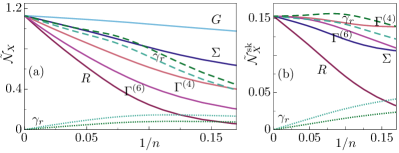
Figure 3: Plots for the rescaled number of (a) bare and (b) skeleton diagrams with $n$ ranging up to $1500$. Numbers are rescaled as $\tilde{\mathcal{N}}_{\Gamma^{(m)}}(n)=\mathcal{N}_{\Gamma^{(m)}}(n)/(n!n^{(m-1)/2}2^{(m-2)/2})$ [Eq. (22)]; $G$ is rescaled in the same way as $\Sigma=\Gamma^{(2)}$ [Eq. (24)]; $R$ and $\gamma_{r}$ ($r=a,p$, dotted) in the same way as $\Gamma^{(4)}$. Dashed lines for $\gamma_{r}$ account for the correct asymptote, showing $\mathcal{N}_{\gamma_{r}}/(4|\sigma_{r}|n!n^{1/2})$ [Eq. (25)].

The $m$ dependence in Eq. (22) can be readily understood from the universal part of the exact fRG flow equations, $\dot{\Gamma}^{(m)}=-\Gamma^{(m+2)}\circ S+\dots$ Metzner et al. (2012); Kopietz et al. (2010). Due to the factorial growth, we have $\mathcal{N}_{X}(n)\gg\mathcal{N}_{X}(n-1)$ for $n\gg 1$, and the leading behavior is determined by [using $\mathcal{N}_{S}(0)=1$ and Eq. (12b)]

$$\mathcal{N}_{\Gamma^{(m+2)}}(n)\mathcal{N}_{S^{\vphantom{(6)}}}(0)\sim\mathcal{N}_{\dot{\Gamma}^{(m)}}(n)\sim 2n\,\mathcal{N}_{\Gamma^{(m)}}(n),\ n\gg 1.$$ (23)

The asymptotes of $G$ and $\Sigma=\Gamma^{(2)}$ agree due to the simple relation deduced from Eq. (10) for $n\gg 1$,

$$\mathcal{N}_{G}(n)\sim\mathcal{N}_{G_{0}}(0)\mathcal{N}_{\Sigma}(n)\mathcal{N}_{G}(0)\sim\mathcal{N}_{\Sigma}(n)\sim n!n^{1/2}.$$ (24)

The number of diagrams in the reducible vertices $\gamma_{r}$ divided by the same function as $\Gamma^{(4)}$ (dotted lines in Fig. 3) go to zero. In fact, the correct asymptote of the reducible vertices (as used for the dashed lines in Fig. 3) is found from the BSEs (19b)

$$\mathcal{N}_{\gamma_{r}}(n) \sim 2|\sigma_{r}|\mathcal{N}_{\Gamma^{(4)}}(1)\mathcal{N}_{G}(0)\mathcal{N}_{G}(0)\mathcal{N}_{\Gamma^{(4)}}(n-1)$$

$$\sim 4|\sigma_{r}|(n-1)!n^{3/2}=4|\sigma_{r}|n!n^{1/2},\ n\gg 1.$$ (25)

According to Eq. (19a), the number of diagrams in the totally irreducible vertex $R$ must then grow as fast as $\mathcal{N}_{\Gamma^{(4)}}$,

$$\mathcal{N}_{R}(n) \sim\mathcal{N}_{\Gamma^{(4)}}(n)\sim 2n!n^{3/2},$$ (26a)

$$\frac{\mathcal{N}_{\gamma_{r}}(n)}{\mathcal{N}_{R}(n)} \sim\frac{2|\sigma_{r}|}{n},\quad n\gg 1.$$ (26b)

From Fig. 3, we indeed see that $\mathcal{N}_{R}>\mathcal{N}_{\gamma_{a}},\mathcal{N}_{\gamma_{p}}$ for $n>8$.

The proportionality factor of roughly $1.128$ in the asymptotics of the bare number of diagrams can be derived from a combinatorial approach to count diagrams in $m$-point connected Green’s function $G^{(m)}$ (with $G=G^{(2)}$). If the recursion relation for $G$ given in Ref. Jishi, 2013 [their Eq. (9.10)] is translated to Hugenholtz diagrams and generalized to $m$-point functions, it reads

$$\mathcal{N}_{G^{(m)}}(n) =\frac{(2n+m/2)!}{n!4^{n}}-\sum_{k=1}^{n}\frac{(2k)!}{k!4^{k}}\mathcal{N}_{G^{(m)}}(n-k),$$ (27)

where the first summand accounts for all topologically distinct contractions and the second summand removes disconnected ones. For the asymptotic behavior, it suffices to subtract the fully disconnected part [the $k=n$ summand dominates since $\mathcal{N}_{X}(n)\gg\mathcal{N}_{X}(n-1)$], and we obtain, using $\mathcal{N}_{G^{(m)}}(0)=\mathit{O}(1)$ and Stirling’s formula,

$$\mathcal{N}_{G^{(m)}}(n) \sim\frac{(2n+m/2)!}{n!4^{n}}-\frac{(2n)!}{n!4^{n}}\sim\frac{(2n)^{m/2}(2n)!}{n!4^{n}}$$

$$\sim\frac{2}{\sqrt{\pi}}n!n^{(m-1)/2}2^{(m-2)/2},\ n\gg 1.$$ (28)

Comparing this to Eq. (22), we indeed find a proportionality factor of $2/\sqrt{\pi}\approx 1.128$ .

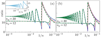
Figure 4: Ratio of subsequent elements of (a) $\mathcal{N}_{X}$ and (b) $\mathcal{N}_{X}^{\textrm{sk}}$ in the parquet-type approximations with $n_{p}=30$ and $n_{p}=12$ (see main text). We use the same color coding as in Fig. 3; dashed lines represent $\gamma_{r}$. The inset shows an analogous plot for $\mathcal{N}_{G}$, obtained from a finite-order self-energy ($n_{s}=20$) [cf. Eq. (29)]. The cusp for $\Gamma^{(4)}$, $\Sigma$, $G$ occurs at $1/n_{p}$ (inset: $1/n_{s}$), and for $\gamma_{r}$ at $1/n_{p}+1$, due to the structure of the BSEs [cf. (19b)].

IV.4 Asymptotics of parquet approximations

In any type of parquet approximation, one has $\mathcal{N}_{R}(n)=0$ for $n>n_{p}$ (i.e., $n_{p}$ denotes the highest-order contribution retained for $R$), whereas the reducible vertices and the self-energy still extend to arbitrarily high orders, as determined by the self-consistent BSEs (7) and SDE (3b). However, in this case, a factorial growth in the number of diagrams [$\mathcal{N}_{X}(n)\gg\mathcal{N}_{X}(n-1)$] leading to Eq. (26) would contradict a vertex $R$ of finite order. Hence, the number of diagrams in any approximation of the parquet type can at most grow exponentially [$\mathcal{N}_{X}(n)/\mathcal{N}_{X}(n-1)\sim\mathit{O}(1)$]. Figure 4 shows how the quotient of two subsequent elements in $\mathcal{N}_{X}$ subject to (two different) parquet-type approximations approaches a constant; it confirms the exponential growth and reveals that the exponential rate only depends on $n_{p}$ for all vertex functions. Curiously, one finds dampened oscillations modulating the growth in the number of diagrams for $n>n_{p}\gtrsim 10$.

An analogous phenomenon already occurs by using the Dyson equation with a self-energy of finite order (cf. Fig. 4, inset). Again, a factorial growth in the number of diagrams [$\mathcal{N}_{X}(n)\gg\mathcal{N}_{X}(n-1)$] leading to Eq. (24) would contradict such an $\mathcal{N}_{\Sigma}$, and $\mathcal{N}_{G}$ can at most grow exponentially. If $\mathcal{N}_{\Sigma}(n)=0$ for $n>n_{s}$, Eq. (8) is simplified to

$$\mathcal{N}_{G}(n)=\delta_{n,0}+\sum_{m=1}^{\textrm{min}\{n,n_{s}\}}\mathcal{N}_{\Sigma}(m)\mathcal{N}_{G}(n-m).$$ (29)

For large $n$, the factor $\mathcal{N}_{G}(n-m)$ spans over the orders $n-n_{s},\dots,n$ and produces “fading echoes” of the abrupt fall in the quotient which stems from the first occurrence of $\mathcal{N}_{\Sigma}(n)=0$ at $n=n_{s}+1$.

Even if only the skeleton diagrams of, e.g., $\Sigma$ or $R$ are of finite order, the resulting numbers of bare diagrams can grow at most exponentially. The reasoning is similar: A factorial growth in the number of diagrams [$\mathcal{N}_{X}(n)\gg\mathcal{N}_{X}(n-1)$] would imply $\mathcal{N}_{\Gamma^{(m)}}(n)\sim\mathcal{N}_{\Gamma^{(m)}}^{\textrm{sk}}(n_{\textrm{min}})\mathcal{N}_{G}(n-n_{\textrm{min}})$, using Eq. (20) and $\mathcal{N}_{G}(0)=1$. For $\Sigma$, one has $n_{\textrm{min}}=1$, and the result would directly contradict Eq. (24). For $R$, one has $n_{\textrm{min}}=4$ and would find a contradiction using Eqs. (23), (24), and (26). We conclude that for any of the typical diagrammatic resummation approaches, one generates numbers of (bare) diagrams that grow at most exponentially with interaction order $n$.

IV.5 Hubbard model

$n$	1	2	3	4	5	6	7
$\mathcal{N}_{\Sigma}$	1	2	8	44	296	2312	20384
$\mathcal{N}_{\Gamma^{(4)}}^{\uparrow\downarrow}$	1	2	13	104	940	9352	101080
$\mathcal{N}_{\gamma_{a}}^{\uparrow\downarrow}$	0	1	5	36	300	2760	27544
$\mathcal{N}_{\gamma_{t}}^{\uparrow\downarrow}$	0	0	3	30	282	2758	28526
$\mathcal{N}_{R}^{\uparrow\downarrow}$	1	0	0	2	58	1074	17466
$\mathcal{N}_{\Gamma^{(4)}}^{\uparrow\uparrow}$	0	2	12	94	848	8468	92016
$\mathcal{N}_{\gamma_{a}}^{\uparrow\uparrow}$	0	1	6	44	366	3354	33334
$\mathcal{N}_{\gamma_{p}}^{\uparrow\uparrow}$	0	0	0	2	28	320	3532
$\mathcal{N}_{R}^{\uparrow\uparrow}$	0	0	0	4	88	1440	21816
$\mathcal{N}_{\Gamma^{(6)}}^{\uparrow\downarrow\uparrow}$	0	0	8	144	2072	28744	402736
$\mathcal{N}_{\Gamma^{(6)}}^{\uparrow\uparrow\uparrow}$	0	0	12	144	1872	25176	349812

Table 3: Exact number of spin-resolved bare diagrams in the Hubbard model. By symmetry, we have $\mathcal{N}_{\gamma_{a}}^{\uparrow\uparrow}=\mathcal{N}_{\gamma_{t}}^{\uparrow\uparrow}$, and one further finds $\mathcal{N}_{\gamma_{a}}^{\uparrow\downarrow}=\mathcal{N}_{\gamma_{p}}^{\uparrow\downarrow}$ [cf. Fig. 5 and Eq. (42)].

The Hubbard model Montorsi (1992) is of special interest in condensed matter physics. In terms of diagrams, a simplification arises due to the SU(2) spin symmetry of the model with the restrictive bare vertex ($\sigma\in\{\uparrow,\downarrow\}$)

$$\Gamma^{(4)}_{0;x_{1}^{\prime},x_{2}^{\prime};x_{1},x_{2}}\propto(\delta_{\sigma_{1}^{\prime},\sigma_{1}^{\phantom{\prime}}}\delta_{\sigma_{2}^{\prime},\sigma_{2}^{\phantom{\prime}}}-\delta_{\sigma_{1}^{\prime},\sigma_{2}^{\phantom{\prime}}}\delta_{\sigma_{2}^{\prime},\sigma_{1}^{\phantom{\prime}}})\,\delta_{\sigma_{1}^{\phantom{\prime}},\bar{\sigma}_{2}^{\phantom{\prime}}},$$ (30)

where $\bar{\uparrow}=\downarrow$, $\bar{\downarrow}=\uparrow$. In this case, one can individually count diagrams with specific spin configuration. In other words, one can explicitly perform the spin sums in all diagrams and actually count only those diagrams that do not vanish under the spin restriction.

$n$	1	2	3	4	5	6	7
$\mathcal{N}_{\Sigma}^{\textrm{sk}}$	1	1	2	9	54	390	3268
$\mathcal{N}_{\Gamma^{(4)}}^{\textrm{sk}\uparrow\downarrow}$	1	2	9	54	390	3268	30905
$\mathcal{N}_{\gamma_{a}}^{\textrm{sk}\uparrow\downarrow}$	0	1	3	17	112	850	7289
$\mathcal{N}_{\gamma_{t}}^{\textrm{sk}\uparrow\downarrow}$	0	0	3	18	120	928	8029
$\mathcal{N}_{R}^{\textrm{sk}\uparrow\downarrow}$	1	0	0	2	46	640	8298
$\mathcal{N}_{\Gamma^{(4)}}^{\textrm{sk}\uparrow\uparrow}$	0	2	8	48	352	2978	28376
$\mathcal{N}_{\gamma_{a}}^{\textrm{sk}\uparrow\uparrow}$	0	1	4	21	136	1028	8768
$\mathcal{N}_{\gamma_{p}}^{\textrm{sk}\uparrow\uparrow}$	0	0	0	2	16	126	1064
$\mathcal{N}_{R}^{\textrm{sk}\uparrow\uparrow}$	0	0	0	4	64	796	9776
$\mathcal{N}_{\Gamma^{(6)}}^{\textrm{sk}\uparrow\downarrow\uparrow}$	0	0	8	120	1376	15648	185296
$\mathcal{N}_{\Gamma^{(6)}}^{\textrm{sk}\uparrow\uparrow\uparrow}$	0	0	12	108	1188	13464	160236

Table 4: Exact number of spin-resolved skeleton diagrams in the Hubbard model, where we again have $\mathcal{N}_{\gamma_{a}}^{\textrm{sk}\uparrow\uparrow}=\mathcal{N}_{\gamma_{t}}^{\textrm{sk}\uparrow\uparrow}$ and $\mathcal{N}_{\gamma_{a}}^{\textrm{sk}\uparrow\downarrow}=\mathcal{N}_{\gamma_{p}}^{\textrm{sk}\uparrow\downarrow}$.

So far, we have considered diagrams that contain summations over all internal degrees of freedom—including spin. Generally, our algorithm cannot give the functional dependence of the diagrams and, in particular, does not give the spin dependence of the diagrams. If one writes the relations stated above with their explicit spin dependence (as done in App. A), one finds that the SDE relates the self-energy to the vertex with different spins at the external legs. However, the differential equations contain a summation over all spin configurations of the vertex. Thus, Eqs. (14) and (16a) cannot be used to deduce the number of spin-resolved vertex diagrams.

As already mentioned, for approximate many-body approaches that do allow for an iterative construction, such as parquet-type approximations, we need not make use of the differential equations. We could therefore easily construct the corresponding numbers of spin-resolved diagrams. However, here, we prefer to give low-order results for the exact numbers of diagrams for all the different vertex functions by resorting to known results: We use exact numbers of diagrams for a specific quantity not considered in this work, which are obtained by Monte Carlo sampling up to order 7 in Ref. Van Houcke et al., (their Table I). From this, we can deduce the number of diagrams in the totally irreducible vertex $R$ and, then, generate the numbers for all further vertex functions studied here.

Using spin symmetry, only a few spin configurations of the vertices are actually relevant: One-particle properties must be independent of spin; for two- and three-particle vertices, it suffices to consider those with identical spins and those with two different pairs of spins. In App. A, we explain the labeling and give further relations that follow from the SU(2) spin symmetry and rely on cancelations of diagrams.

Table 3 gives the exact number of bare diagrams for the Hubbard model up to order 7; Table 4 gives the corresponding numbers of skeleton diagrams. The numbers for $\mathcal{N}_{\Sigma}^{\textrm{sk}}$ up to order 6 agree with those of Ref. Zhou, 2008 (their Table 4.1, column 3). Note that, for spin-resolved diagrams of the Hubbard model, we can use the internal spin summations to express all Hugenholtz diagrams in terms of the bare vertex $\Gamma_{0}^{\uparrow\downarrow}$ with fixed spins, containing only one diagram. Hence, the number of spin-resolved Hugenholtz and Feynman diagrams for this model are equal (cf. Fig. 5).

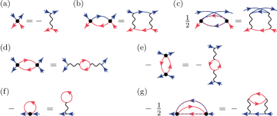
Figure 5: Spin-resolved diagrams of the Hubbard model in the Hugenholtz and Feynman representation up to second order. Blue (dark) lines denote spin-up and red (light) lines spin-down propagators; dashed lines symbolize a sum over spin. Panels (a)–(c) give diagrams for $\Gamma_{0}^{\uparrow\downarrow}$, $\gamma_{a}^{\uparrow\downarrow}$, and $\gamma_{p}^{\uparrow\downarrow}$; (d)–(e) for $\gamma_{a}^{\uparrow\uparrow}$, and $\gamma_{t}^{\uparrow\uparrow}$; (f)–(g) for $\Sigma$. Viewed with full propagators, these are all skeleton diagrams entering $\Gamma^{(4)}$ and $\Sigma$ up to second order. We explicitly see that the numbers of Hugenholtz and Feynman diagrams are equal.

It is interesting to compare the number of diagrams in the four-point vertex with identical and different spins. On top of the numbers given in Tables 3 and 4, our algorithm can also determine the asymptotic behavior of, e.g., the relation between $\mathcal{N}_{\Gamma^{(4)}}^{\uparrow\uparrow}$ and $\mathcal{N}_{\Gamma^{(4)}}^{\uparrow\downarrow}$. If we consider skeleton diagrams, the SDE (40a) with $\mathcal{N}_{\Gamma^{(4)}_{0}}^{\textrm{sk}\uparrow\downarrow}(n)=\delta_{n,1}$ yields $\mathcal{N}_{\Sigma}^{\textrm{sk}}(n+1)=\mathcal{N}_{\Gamma^{(4)}}^{\textrm{sk}\uparrow\downarrow}(n)$. Combined with the (super) factorial growth of $\mathcal{N}_{\Sigma}^{\textrm{sk}}$, this gives

$$n\mathcal{N}_{\Sigma}^{\textrm{sk}}(n)\gtrsim\mathcal{N}_{\Sigma}^{\textrm{sk}}(n+1)=\mathcal{N}_{\Gamma^{(4)}}^{\textrm{sk}\uparrow\downarrow}(n),\quad n\gg 1.$$ (31)

On the other hand, Eq. (12b) and Eq. (40c) together with the knowledge that $\mathcal{N}_{R}$ asymptotically dominates $\mathcal{N}_{\Gamma^{(4)}}$ can be used to obtain

$$2n\mathcal{N}_{\Sigma}^{\textrm{sk}}(n) \lesssim\mathcal{N}_{I_{t}}^{\textrm{sk}\uparrow\uparrow}(n)+\mathcal{N}_{I_{t}}^{\textrm{sk}\uparrow\downarrow}(n)$$

$$\lesssim\mathcal{N}_{\Gamma^{(4)}}^{\textrm{sk}\uparrow\uparrow}(n)+\mathcal{N}_{\Gamma^{(4)}}^{\textrm{sk}\uparrow\downarrow}(n),\quad n\gg 1.$$ (32)

Dividing both equations, we find that, according to

$$\mathcal{N}_{\Gamma^{(4)}}^{\uparrow\uparrow}(n)/\mathcal{N}_{\Gamma^{(4)}}^{\uparrow\downarrow}(n)\sim\mathcal{N}_{\Gamma^{(4)}}^{\textrm{sk}\uparrow\uparrow}(n)/\mathcal{N}_{\Gamma^{(4)}}^{\textrm{sk}\uparrow\downarrow}(n)\gtrsim 1,\quad n\gg 1,$$ (33)

the number of diagrams for the effective interaction between same spins asymptotically approaches the one between different spins from above for large interaction orders.

V Conclusion

We have presented an iterative algorithm to count the number of Feynman diagrams inherent in many-body integral equations. We have used it to count the exact number of bare and skeleton diagrams in various vertex function and different two-particle channels. Our algorithm can easily be applied to many-body relations of different forms and levels of approximation, such as the parquet formalism Bickers (2004); Roulet et al. (1969) and its simplified variant FLEX Bickers (2004), other approaches based on Hedin’s equations Hedin (1965); Molinari and Manini (2006) including the famous GW approximation Aryasetiawan and Gunnarsson (1998); Molinari (2005), $\Phi$-derivable results deduced from a specific approximation of the Luttinger-Ward functional Bickers (2004); Luttinger and Ward (1960); Baym (1962), and truncated flows of the functional renormalization group Metzner et al. (2012); Kopietz et al. (2010); Kugler and von Delft (2018b, a).

Due to its iterative structure, the algorithm allows us to numerically access arbitrarily large interaction orders and gain analytical insight into the asymptotic behavior. First, we have extracted a leading dependence of $n!n^{(m-1)/2}2^{(m-2)/2}$ in the number of diagrams of an $m$-point 1PI vertex. Second, we have shown that the number of diagrams in the totally irreducible four-point vertex exceeds those of the reducible ones for interaction orders $n>8$ and asymptotically contains all diagrams of the four-point vertex [i.e., $\mathcal{N}_{\gamma_{r}}(n)/\mathcal{N}_{R}(n)\to 0$ as $n\to\infty$]. Third, we have argued that any of the typical diagrammatic resummation procedures, including any type of parquet approximation, can support an exponential growth only in the number of diagrams. This is in contrast to the factorial growth in the exact number of diagrams. It is therefore likely that the corresponding approximate series expansions do have a finite radius of convergence.

We believe that the techniques and results presented in this paper will be useful for various applications of Green’s-functions methods as well as approaches that directly sum diagrams, such as finite-order approximations or diagrammatic Monte Carlo Houcke et al. (2010).

Appendix A Relations for the Hubbard model

The spin symmetry in the Hubbard model allows us to focus on a small set of vertex functions when counting diagrams. By spin conservation, an $n$-particle vertex depends on only $n$ spins. Using the $\mathbb{Z}_{2}$ symmetry, it is clear that self-energy diagrams do not depend on spin, while, for the four-point vertex, it suffices to consider

$$\mathcal{N}_{\Gamma^{(4)}}^{\uparrow\uparrow}:=\mathcal{N}_{\Gamma^{(4)}}^{\uparrow\uparrow;\uparrow\uparrow},\quad\mathcal{N}_{\Gamma^{(4)}}^{\uparrow\downarrow}:=\mathcal{N}_{\Gamma^{(4)}}^{\uparrow\downarrow;\uparrow\downarrow}.$$ (34)

Here, we write the spin indices of the vertex in the order of Eq. (1) as superscripts of $\mathcal{N}$. The classification of four-point diagrams into two-particle channels depends on the labels of the external legs. By crossing symmetry, we have $\mathcal{N}_{\gamma_{a}}^{\uparrow\uparrow}=\mathcal{N}_{\gamma_{t}}^{\uparrow\uparrow}$ and find for different spins

$$\mathcal{N}_{\gamma_{p}}^{\uparrow\downarrow} :=\mathcal{N}_{\gamma_{p}}^{\uparrow\downarrow;\uparrow\downarrow}=\mathcal{N}_{\gamma_{p}}^{\uparrow\downarrow;\downarrow\uparrow},$$ (35a)

$$\mathcal{N}_{\gamma_{a}}^{\uparrow\downarrow} :=\mathcal{N}_{\gamma_{a}}^{\uparrow\downarrow;\uparrow\downarrow}=\mathcal{N}_{\gamma_{t}}^{\uparrow\downarrow;\downarrow\uparrow},$$ (35b)

$$\mathcal{N}_{\gamma_{t}}^{\uparrow\downarrow} :=\mathcal{N}_{\gamma_{t}}^{\uparrow\downarrow;\uparrow\downarrow}=\mathcal{N}_{\gamma_{a}}^{\uparrow\downarrow;\downarrow\uparrow}.$$ (35c)

For the six-point vertex, we need to consider only (the semicolon again separates incoming and outgoing lines)

$$\mathcal{N}_{\Gamma^{(6)}}^{\uparrow\uparrow\uparrow}:=\mathcal{N}_{\Gamma^{(6)}}^{\uparrow\uparrow\uparrow;\uparrow\uparrow\uparrow},\quad\mathcal{N}_{\Gamma^{(6)}}^{\uparrow\downarrow\uparrow}:=\mathcal{N}_{\Gamma^{(6)}}^{\uparrow\downarrow\uparrow;\uparrow\downarrow\uparrow}.$$ (36)

The SU(2) spin symmetry further relates the remaining components of the four-point vertex by Rohringer et al. (2012)

$$\Gamma^{(4)}_{p^{\prime}\uparrow,q^{\prime}\uparrow;p^{\vphantom{\prime}}\uparrow,q^{\vphantom{\prime}}\uparrow}=\Gamma^{(4)}_{p^{\prime}\uparrow,q^{\prime}\downarrow;p^{\vphantom{\prime}}\downarrow,q^{\vphantom{\prime}}\uparrow}-\Gamma^{(4)}_{p^{\prime}\uparrow,q^{\prime}\downarrow;q^{\vphantom{\prime}}\downarrow,p^{\vphantom{\prime}}\uparrow},$$ (37)

where we have decomposed the quantum number $x$ into $p$ and $\sigma$. However, this subtraction involves cancelations of diagrams as opposed to the summation of topologically distinct, independent diagrams we have encountered so far. This can already be seen at first order where $\mathcal{N}_{\Gamma^{(4)}_{0}}^{\uparrow\uparrow}=0$. Such cancelations of diagrams can only change the number of diagrams by a multiple of 2. Consequently, we infer that

$$2\mathcal{N}_{\Gamma^{(4)}}^{\uparrow\downarrow}-\mathcal{N}_{\Gamma^{(4)}}^{\uparrow\uparrow}\in 2\mathbb{N}_{0}.$$ (38)

If we further invoke the channel decomposition with crossing symmetries, we find that all of

$$2\mathcal{N}_{R}^{\uparrow\downarrow}-\mathcal{N}_{R}^{\uparrow\uparrow},\quad 2\mathcal{N}_{\gamma_{p}}^{\uparrow\downarrow}-\mathcal{N}_{\gamma_{p}}^{\uparrow\uparrow},\quad\mathcal{N}_{\gamma_{a}}^{\uparrow\downarrow}+\mathcal{N}_{\gamma_{t}}^{\uparrow\downarrow}-\mathcal{N}_{\gamma_{a}}^{\uparrow\uparrow}$$ (39)

are nonnegative, even numbers (as can explicitly be checked in Tables 3 and 4).

Next, we perform the spin summation in the different many-body relations stated in Sec. III. Starting with Eqs. (11) and (13) for the self-energy, we get

$$\mathcal{N}_{\Sigma} =\mathcal{N}_{\Gamma^{(4)}_{0}}^{\uparrow\downarrow}\ast\mathcal{N}_{G}+\mathcal{N}_{\Gamma^{(4)}_{0}}^{\uparrow\downarrow}\ast\mathcal{N}_{\Pi}\ast\mathcal{N}_{G}\ast\mathcal{N}_{\Gamma^{(4)}}^{\uparrow\downarrow},$$ (40a)

$$\mathcal{N}_{\dot{\Sigma}} =(\mathcal{N}_{\Gamma^{(4)}}^{\uparrow\downarrow}+\mathcal{N}_{\Gamma^{(4)}}^{\uparrow\uparrow})\ast\mathcal{N}_{S}$$ (40b)

$$=(\mathcal{N}_{I_{t}}^{\uparrow\downarrow}+\mathcal{N}_{I_{t}}^{\uparrow\uparrow})\ast\mathcal{N}_{\dot{G}}.$$ (40c)

From Eqs. (17) and (18), we similarly get for the four-point vertex ($\mathcal{N}_{\dot{\Pi}_{S}}=\mathcal{N}_{G}\ast\mathcal{N}_{S}$)

$$\mathcal{N}_{\dot{\Gamma}^{(4)}}^{\uparrow\downarrow} =2\,\mathcal{N}_{\Gamma^{(4)}}^{\uparrow\downarrow}\ast\mathcal{N}_{\dot{\Pi}_{S}}\ast\mathcal{N}_{\Gamma^{(4)}}^{\uparrow\downarrow}+2\,\mathcal{N}_{\Gamma^{(4)}}^{\uparrow\downarrow}\ast\mathcal{N}_{\dot{\Pi}_{S}}\ast\mathcal{N}_{\Gamma^{(4)}}^{\uparrow\uparrow}$$

$$\ +2\,\mathcal{N}_{\Gamma^{(6)}}^{\uparrow\downarrow\uparrow}\ast N_{S},$$ (41a)

$$\mathcal{N}_{\dot{\Gamma}^{(4)}}^{\uparrow\uparrow} =\tfrac{5}{2}\,\mathcal{N}_{\Gamma^{(4)}}^{\uparrow\uparrow}\ast\mathcal{N}_{\dot{\Pi}_{S}}\ast\mathcal{N}_{\Gamma^{(4)}}^{\uparrow\uparrow}+2\,\mathcal{N}_{\Gamma^{(4)}}^{\uparrow\downarrow}\ast\mathcal{N}_{\dot{\Pi}_{S}}\ast\mathcal{N}_{\Gamma^{(4)}}^{\uparrow\downarrow}$$

$$\ +\mathcal{N}_{\Gamma^{(6)}}^{\uparrow\downarrow\uparrow}\ast N_{S}+\mathcal{N}_{\Gamma^{(6)}}^{\uparrow\uparrow\uparrow}\ast N_{S},$$ (41b)

$$\mathcal{N}_{\Gamma^{(4)}}^{\uparrow\downarrow} =\mathcal{N}_{\Gamma^{(4)}_{0}}^{\uparrow\downarrow}+2\,\mathcal{N}_{\Gamma^{(4)}_{0}}^{\uparrow\downarrow}\ast\mathcal{N}_{\Pi}\ast\mathcal{N}_{\Gamma^{(4)}}^{\uparrow\downarrow}$$

$$\ +\mathcal{N}_{\Gamma^{(4)}_{0}}^{\uparrow\downarrow}\ast\mathcal{N}_{\Pi}\ast\mathcal{N}_{\Gamma^{(4)}}^{\uparrow\uparrow}+\mathcal{N}_{\Gamma^{(4)}_{0}}^{\uparrow\downarrow}\ast\mathcal{N}_{\Pi}\ast\mathcal{N}_{\Gamma^{(6)}}^{\uparrow\downarrow\uparrow}$$

$$\ +3\,\mathcal{N}_{\Gamma^{(4)}_{0}}^{\uparrow\downarrow}\ast\mathcal{N}_{\Pi}\ast\mathcal{N}_{\Pi}\ast\mathcal{N}_{\Gamma^{(4)}}^{\uparrow\downarrow}\ast\mathcal{N}_{\Gamma^{(4)}}^{\uparrow\downarrow}$$

$$\ +4\,\mathcal{N}_{\Gamma^{(4)}_{0}}^{\uparrow\downarrow}\ast\mathcal{N}_{\Pi}\ast\mathcal{N}_{\Pi}\ast\mathcal{N}_{\Gamma^{(4)}}^{\uparrow\downarrow}\ast\mathcal{N}_{\Gamma^{(4)}}^{\uparrow\uparrow},$$ (41c)

$$\mathcal{N}_{\Gamma^{(4)}}^{\uparrow\uparrow} =2\,\mathcal{N}_{\Gamma^{(4)}_{0}}^{\uparrow\downarrow}\ast\mathcal{N}_{\Pi}\ast\mathcal{N}_{\Gamma^{(4)}}^{\uparrow\downarrow}$$

$$\ +\mathcal{N}_{\Gamma^{(4)}_{0}}^{\uparrow\downarrow}\ast\mathcal{N}_{\Pi}\ast\mathcal{N}_{\Gamma^{(4)}}^{\uparrow\uparrow}+\mathcal{N}_{\Gamma^{(4)}_{0}}^{\uparrow\downarrow}\ast\mathcal{N}_{\Pi}\ast\mathcal{N}_{\Gamma^{(6)}}^{\uparrow\downarrow\uparrow}$$

$$\ +4\,\mathcal{N}_{\Gamma^{(4)}_{0}}^{\uparrow\downarrow}\ast\mathcal{N}_{\Pi}\ast\mathcal{N}_{\Pi}\ast\mathcal{N}_{\Gamma^{(4)}}^{\uparrow\downarrow}\ast\mathcal{N}_{\Gamma^{(4)}}^{\uparrow\downarrow}$$

$$\ +3\,\mathcal{N}_{\Gamma^{(4)}_{0}}^{\uparrow\downarrow}\ast\mathcal{N}_{\Pi}\ast\mathcal{N}_{\Pi}\ast\mathcal{N}_{\Gamma^{(4)}}^{\uparrow\downarrow}\ast\mathcal{N}_{\Gamma^{(4)}}^{\uparrow\uparrow}.$$ (41d)

Finally, we resolve the parquet equations (19) in their spin configurations and obtain

$$\mathcal{N}_{\Gamma^{(4)}}^{\sigma\sigma^{\prime}} =\mathcal{N}_{R}^{\sigma\sigma^{\prime}}+\textstyle{\sum_{r}}\mathcal{N}_{\gamma_{r}}^{\sigma\sigma^{\prime}},$$ (42a)

$$\mathcal{N}_{I_{r}}^{\sigma\sigma^{\prime}} =\mathcal{N}_{\Gamma^{(4)}}^{\sigma\sigma^{\prime}}-\mathcal{N}_{\gamma_{r}}^{\sigma\sigma^{\prime}},$$ (42b)

$$\mathcal{N}_{\gamma_{a}}^{\uparrow\downarrow} =\mathcal{N}_{I_{a}}^{\uparrow\downarrow}\ast\mathcal{N}_{\Pi}\ast\mathcal{N}_{\Gamma^{(4)}}^{\uparrow\downarrow},$$ (42c)

$$\mathcal{N}_{\gamma_{p}}^{\uparrow\downarrow} =\mathcal{N}_{I_{p}}^{\uparrow\downarrow}\ast\mathcal{N}_{\Pi}\ast\mathcal{N}_{\Gamma^{(4)}}^{\uparrow\downarrow},$$ (42d)

$$\mathcal{N}_{\gamma_{t}}^{\uparrow\downarrow} =\mathcal{N}_{I_{t}}^{\uparrow\downarrow}\ast\mathcal{N}_{\Pi}\ast\mathcal{N}_{\Gamma^{(4)}}^{\uparrow\uparrow}+\mathcal{N}_{I_{t}}^{\uparrow\uparrow}\ast\mathcal{N}_{\Pi}\ast\mathcal{N}_{\Gamma^{(4)}}^{\uparrow\downarrow},$$ (42e)

$$\mathcal{N}_{\gamma_{a}}^{\uparrow\uparrow} =\mathcal{N}_{I_{a}}^{\uparrow\uparrow}\ast\mathcal{N}_{\Pi}\ast\mathcal{N}_{\Gamma^{(4)}}^{\uparrow\uparrow}+\mathcal{N}_{I_{t}}^{\uparrow\downarrow}\ast\mathcal{N}_{\Pi}\ast\mathcal{N}_{\Gamma^{(4)}}^{\uparrow\downarrow},$$ (42f)

$$\mathcal{N}_{\gamma_{p}}^{\uparrow\uparrow} =\tfrac{1}{2}\mathcal{N}_{I_{p}}^{\uparrow\uparrow}\ast\mathcal{N}_{\Pi}\ast\mathcal{N}_{\Gamma^{(4)}}^{\uparrow\uparrow},$$ (42g)

$$\mathcal{N}_{\gamma_{t}}^{\uparrow\uparrow} =\mathcal{N}_{I_{t}}^{\uparrow\uparrow}\ast\mathcal{N}_{\Pi}\ast\mathcal{N}_{\Gamma^{(4)}}^{\uparrow\uparrow}+\mathcal{N}_{I_{t}}^{\uparrow\downarrow}\ast\mathcal{N}_{\Pi}\ast\mathcal{N}_{\Gamma^{(4)}}^{\uparrow\downarrow}.$$ (42h)

In Sec. III, we combined the Schwinger-Dyson with differential (or flow) equations to iteratively construct the exact number of diagrams. Here, we see that the Schwinger-Dyson equations of $\Sigma$ [Eq. (40a)] and $\Gamma^{(4)}$ [Eqs. (41c) and (41d)] contain the corresponding higher-point vertex $\Gamma^{(4)}$ and $\Gamma^{(6)}$, respectively, only in the configuration with different spins. However, the differential equations [Eqs. (40b) and (40c) and Eqs. (41a) and (41b)] involve the same higher-point vertex in all of its spin configurations. It is for this reason that one cannot iteratively construct the exact number of spin-resolved diagrams. However, the equations can easily be used to generate the number of diagrams in approximations that do allow for an iterative construction, such as parquet-type approximations or approximations that involve a finite number of known (bare or skeleton) diagrams.

References

- Negele and Orland (1998) J. Negele and H. Orland, Quantum Many-particle Systems, Advanced Books Classics (Perseus Books, New York, 1998).
- Kugler and von Delft (2018a) F. B. Kugler and J. von Delft, Phys. Rev. B 97, 035162 (2018a).
- Smith (1992) R. A. Smith, Phys. Rev. A 46, 4586 (1992).
- Hedin (1965) L. Hedin, Phys. Rev. 139, A796 (1965).
- Bickers (2004) N. Bickers, in Theoretical Methods for Strongly Correlated Electrons, CRM Series in Mathematical Physics, edited by D. Sénéchal, A.-M. Tremblay, and C. Bourbonnais (Springer, New York, 2004) pp. 237–296.
- Held et al. (2011) K. Held, C. Taranto, G. Rohringer, and A. Toschi, in The LDA+DMFT Approach to Strongly Correlated Materials – Lecture Notes of the Autumn School 2011, edited by E. Pavarini, E. Koch, D. Vollhardt, and A. Lichtenstein (Forschungszentrum Jülich, Jülich, 2011) Chap. 13.0.
- (7) F. B. Kugler and J. von Delft, arXiv:1807.02898 .
- Note (1) The precise formulation can be found in Ref. \rev@citealpKugler2017a; the indices in the functional derivative are .
- Metzner et al. (2012) W. Metzner, M. Salmhofer, C. Honerkamp, V. Meden, and K. Schönhammer, Rev. Mod. Phys. 84, 299 (2012).
- Kopietz et al. (2010) P. Kopietz, L. Bartosch, and F. Schütz, Introduction to the Functional Renormalization Group (Lect. Notes Phys. 798) (Springer, Berlin, 2010).
- Roulet et al. (1969) B. Roulet, J. Gavoret, and P. Nozières, Phys. Rev. 178, 1072 (1969).
- Note (2) The term transverse refers to a horizontal space-time axis; in using the terms antiparallel and parallel, we adopt the nomenclature used by Roulet et al. Roulet et al. (1969). Equivalently, a common notation Rohringer et al. (2012, 2018); Wentzell et al. for the channels is , referring to the (longitudinal) particle-hole, the particle-particle, and the transverse (or vertical) particle-hole channel, respectively. One also finds the labels in the literature Jakobs et al. (2010), referring to the so-called exchange, pairing, and direct channel, respectively.
- Rohringer et al. (2012) G. Rohringer, A. Valli, and A. Toschi, Phys. Rev. B 86, 125114 (2012).
- Rohringer et al. (2018) G. Rohringer, H. Hafermann, A. Toschi, A. A. Katanin, A. E. Antipov, M. I. Katsnelson, A. I. Lichtenstein, A. N. Rubtsov, and K. Held, Rev. Mod. Phys. 90, 025003 (2018).
- (15) N. Wentzell, G. Li, A. Tagliavini, C. Taranto, G. Rohringer, K. Held, A. Toschi, and S. Andergassen, arXiv:1610.06520 .
- Jakobs et al. (2010) S. G. Jakobs, M. Pletyukhov, and H. Schoeller, Phys. Rev. B 81, 195109 (2010).
- Veschgini and Salmhofer (2013) K. Veschgini and M. Salmhofer, Phys. Rev. B 88, 155131 (2013).
- Cvitanović et al. (1978) P. Cvitanović, B. Lautrup, and R. B. Pearson, Phys. Rev. D 18, 1939 (1978).
- Jishi (2013) R. A. Jishi, Feynman Diagram Techniques in Condensed Matter Physics (Cambridge University Press, Cambridge, 2013).
- Molinari and Manini (2006) L. G. Molinari and N. Manini, Eur. Phys. J. B 51, 331 (2006).
- Zhou (2008) W. Zhou, Ph.D. thesis, University of Georgia, Athens (2008).
- Note (3) Their number at order 6 should be 12018 instead of 12081.
- Note (4) We conclude that in Ref. \rev@citealpCvitanovic1978, Table I, first column, the factor should read instead of . We can numerically confirm their coefficients and for the subleading contributions.
- Montorsi (1992) A. Montorsi, The Hubbard Model: A Reprint Volume (World Scientific, Singapore, 1992).
- (25) K. Van Houcke, F. Werner, N. Prokof’ev, and B. Svistunov, arXiv:1305.3901 .
- Aryasetiawan and Gunnarsson (1998) F. Aryasetiawan and O. Gunnarsson, Reports on Progress in Physics 61, 237 (1998).
- Molinari (2005) L. G. Molinari, Phys. Rev. B 71, 113102 (2005).
- Luttinger and Ward (1960) J. M. Luttinger and J. C. Ward, Phys. Rev. 118, 1417 (1960).
- Baym (1962) G. Baym, Phys. Rev. 127, 1391 (1962).
- Kugler and von Delft (2018b) F. B. Kugler and J. von Delft, Phys. Rev. Lett. 120, 057403 (2018b).
- Houcke et al. (2010) K. V. Houcke, E. Kozik, N. Prokof’ev, and B. Svistunov, Phys. Procedia 6, 95 (2010), Computer Simulations Studies in Condensed Matter Physics XXI.