The Continuing Story of the Wobbling Kink

Abstract

The wobbling kink is the soliton of the $\phi^{4}$ model with an excited internal mode. We outline an asymptotic construction of this particle-like solution that takes into account the coexistence of several space and time scales. The breakdown of the asymptotic expansion at large distances is prevented by introducing the long-range variables “untied” from the short-range oscillations. We formulate a quantitative theory for the fading of the kink’s wobbling due to the second-harmonic radiation, explain the wobbling mode’s longevity and discuss ways to compensate the radiation losses. The compensation is achieved by the spatially uniform driving of the kink, external or parametric, at a variety of resonant frequencies. For the given value of the driving strength, the largest amplitude of the kink’s oscillations is sustained by the parametric pumping — at its natural wobbling frequency. This type of forcing also produces the widest Arnold tongue in the “driving strength versus driving frequency” parameter plane. As for the external driver with the same frequency, it brings about an interesting rack and pinion mechanism that converts the energy of external oscillation to the translational motion of the kink.

1 Prologue

An unlikely insomniac wandering into the Dubna computer centre on one of those freezing nights in the winter of 1975, would invariably see the same slim figure rushing among mainframe dashboards, magnetic tape recorders and card perforation devices. A houndstooth blazer favoured by the jazzmen of the time, a ginger beard and a trademark cigarette holder — with some amazement, the passer-by would recognise Boris (“Bob”) Getmanov, a pianist and a popular character of the local music scene. This time, experimenting with harmonies of nonlinear waves.

The object that inspired Bob’s syncopations, was a $\phi^{4}$ kink with a nonlinearly excited internal mode — something he interpreted as a bound state of three kinks and called a musical term tritone BG4 . In this note we review the continuation of the tritone story — the line of research started with blue sky experiments of an artist captivated by mysteries of the nonlinear world.

2 Wobbling mode

Getmanov’s numerical experiments were motivated by similarities between the $\phi^{4}$-theory and the sine-Gordon model — arguably, the two simplest Lorentz-invariant nonlinear PDEs. While the $\phi^{4}$ and sine-Gordon have so much in common, there is an important difference between the two systems. The sine-Gordon is completely integrable whereas the $\phi^{4}$ model is not. Many a theorist tried to detect at least some remnants of integrability among the properties of the $\phi^{4}$ kinks — and Getmanov with his computer codes was part of that gold rush — but only to find more and more deviations from the exact rules set by the sine-Gordon template.

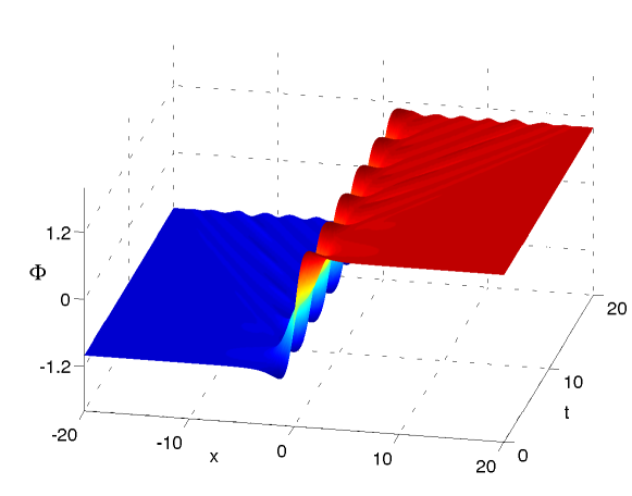
Figure 1: The wobbling kink: a kink with an activated internal mode. This solution was obtained by the numerical simulation of the equation (1) with the initial conditions $\phi_{t}(x,0)=0$ and $\phi(x,0)=\tanh x+2a\tanh x\,\mathrm{sech}\,x$, where $a=0.3$.

One attribute that makes the $\phi^{4}$ kink particularly different from its sine-Gordon twin, is the availability of an internal, or shape, mode. (See Fig 1.) This oscillatory degree of freedom may store energy and release it periodically — giving rise to resonances in the kink-antikink KA ; Belova ; Uspekhi and kink-impurity interactions Uspekhi ; FKV , as well as stimulating kink-antikink pair production MM ; Rom2 . The internal mode serves as the cause of the kink’s counter-intuitive responses to spatially-uniform time-periodic forcing Sukstanskii ; OB and brings about its quasiperiodic velocity oscillations when the kink is set to propagate in a periodic substrate potential Konotop . The excitation of the shape mode also provides a mechanism for the loss of energy and deceleration of the kink moving in a random medium Malomed .

In his simulations, Getmanov observed an amazing longevity of the kink’s large-amplitude oscillations BG4 . The kink seemed to be a comfortable location for the nonlinearity and dispersion to remain balanced in a high-energy excitation. Getmanov regarded the nonlinear excitation of the kink as a metastable bound state of three kinks — for this object was a product of a symmetric collision of two kinks and an antikink. (For more recent simulations of the bound-state formation, see Belova .) This interpretation is consistent with the spontaneous production of a kink-antikink pair when the amplitude of excitation exceeds a certain threshold; see Fig 2.

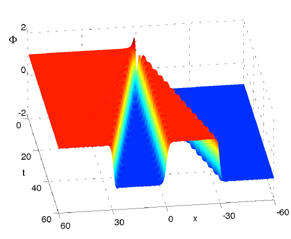
Figure 2: Evolution of the same initial condition as in Fig 1 but with $a=0.6$. An attempt to excite the wobbling mode with a large amplitude results in the emission of a kink-antikink pair. (Note that time flows back to front in this figure.)

Getmanov’s report of his tritone BG4 was eclipsed by the storm of hype around the concurrent discovery of three-dimensional pulsons — in the same equation pulsons . A more sustainable wave of interest starts forming when the one-dimensional $\phi^{4}$ theory,

$$\frac{1}{2}\phi_{tt}-\frac{1}{2}\phi_{xx}-\phi+\phi^{3}=0,$$ (1)

was put forward as a model for the charge-density wave materials CDW . It has become clear that tritones should contribute to all characteristics of the material — alongside kinks and breathers. Rice and Mele described the tritone variationally, using the kink’s width as the dynamical variable Rice1 ; Rice2 . Segur tried to construct this particle-like solution as a regular perturbation expansion in powers of the oscillation amplitude Segur . He determined the first two orders of the expansion (linear and quadratic), noted that expansion should become nonuniform at the order $\epsilon^{3}$ and suggested a possible way to restore the uniformity. To capture the antisymmetric character of oscillations, Segur referred to the tritone simply as the “wobbling kink”.

Another interest group that has always kept an eye on the $\phi^{4}$ kink as the simplest topological soliton, is the particle theorists. Unaware of Segur’s analysis, Arodź and his students developed a regular perturbation expansion using a polynomial approximation in the interior of the kink (see polynomial and references therein) and extended the perturbation theory to the kink embedded in $3+1$ dimensions Pelka . Romańczukiewicz obtained an asymptotic solution for the radiation wave emitted by the wobbling mode that is initially at rest Rom1 and discovered kink-antiknk pair productions stimulated by the wobbling-radiation coupling Rom2 .

Segur’s suggestion for the circumventing of the perturbation breakdown, was to recognise the nonlinear nature of the wobbling mode by expanding its frequency in powers of its amplitude. This recipe constitutes the Lindstedt method in the theory of nonlinear oscillations; in the wobbling kink context this approach was later implemented by Manton and Merabet MM . The Manton-Merabet analysis was successful in reproducing the $t^{-1/2}$ wobbling decay law that had been predicted by Malomed Malomed , on the basis of energy considerations. (See also Rom1 .)

The Lindstedt method is known to be limited even when it is applied to solutions of ordinary differential equations. It proves to be a powerful tool for the calculation of anharmonic corrections to periodic orbits — but fails when the motion ceases to be periodic. More importantly, the method is not well suited for the analysis of partial differential equations — for it cannot handle the nonperiodic spatial degrees of freedom.

One alternative to the Lindstedt method is the Krylov-Bogolyubov collective-coordinate technique. This was used by Kiselev to obtain solutions of the $\phi^{4}$ equation with a perturbed-kink initial condition posed on a characteristic line Kiselev . Although the introduction of collective coordinates allows one to recognise the hierarchy of coexisting space and time scales in the system, the resulting solutions lack the explicitness and transparency of the perturbation expansions in MM ; Segur ; Pelka ; Rom1 . The physical interpretation of their constituents is not straightforward either.

To preserve the lucidity of the regular expansion and, at the same time, take into account the coexistence of multiple space and time scales, Oxtoby and the present author have designed a singular perturbation expansion treating different space and time variables as independent OB ; BO . This asymptotic construction is reviewed in what follows. We also discuss the effects of the resonant forcing of the internal mode by a variety of direct and parametric driving agents.

The emphasis of the present note is on the fundamentals of our method, including the treatment of radiation, and the phenomenology of the wobbling kink’s responses to driving. The reader interested in mathematical detail is wellcome to consult the original publications OB ; BO .

The outline of this chapter is as follows. In the next section we explain the basics of our approach as applied to the freely wobbling kink. Section 4 considers the equation for the wobbling amplitude and draws conclusions on the lifetime of this particle-like excitation. In section 5 we formulate the asymptotic formalism for the consistent treatment of the long-range radiation. Section 6 is devoted to the effect of spatially-uniform temporally-resonant driving force. Some concluding remarks are made in section 7.

3 Multiple scales: slow times and long distances

In this and the next two sections we follow Ref BO . Instead of studying the kink travelling with the velocity $v$, we consider a motionless kink centred at the origin of the reference frame that moves with the velocity $v$ itself. This is accomplished by the change of variables $(x,t)\to(\xi,\tau)$, where $\xi=x-\int_{0}^{t}v(t^{\prime})dt^{\prime}$, $\tau=t$. The above transformation takes equation (1) to

$$\frac{1}{2}\phi_{\tau\tau}-v\phi_{\xi\tau}-\frac{v_{\tau}}{2}\phi_{\xi}-\frac{1-v^{2}}{2}\phi_{\xi\xi}-\phi+\phi^{3}=0.$$ (2)

An explicit occurrence of the soliton velocity in a relativistically-invariant equation is justifiable when there are factors that can induce time-dependence of $v$ (e.g. radiation losses) or when the Lorentz invariance is broken by damping and driving terms. (These are discussed in section 6.)

We expand $\phi$ about the kink $\phi_{0}\equiv\tanh\xi$:

$$\phi=\phi_{0}+\epsilon\phi_{1}+\epsilon^{2}\phi_{2}+\ldots.$$ (3)

Here $\epsilon$ is not pegged to any small parameter of the system (e.g. distance to some critical value) and has the meaning of the amplitude of the kink’s perturbation. It can be chosen arbitrarily.

We also introduce a sequence of “long” space and “slow” time coordinates:

$$X_{n}\equiv\epsilon^{n}\xi,\quad T_{n}\equiv\epsilon^{n}\tau,\quad n=0,1,2,....$$

In the limit $\epsilon\to 0$, the $X_{n}$ and $T_{n}$ are not coupled and can be treated as independent variables. Consequently, the $\xi$- and $\tau$-derivatives are expressible using the chain rule:

$$\frac{\partial}{\partial\xi}=\partial_{0}+\epsilon\partial_{1}+\epsilon^{2}\partial_{2}+\ldots,\quad\frac{\partial}{\partial\tau}=D_{0}+\epsilon D_{1}+\epsilon^{2}D_{2}+\ldots,$$ (4)

where $\partial_{n}\equiv\partial/\partial X_{n}$ and $D_{n}\equiv\partial/\partial T_{n}$.

We limit our analysis to the situation where the velocity is small. Hence we write $v=\epsilon V$ where $V$ is of order 1. Furthermore, when the wobbling amplitude $\epsilon$ is small, it is natural to expect the velocity of the kink to vary slowly. Accordingly, $V$ is taken to be a function of slow times only: $V=V(T_{1},T_{2},...)$.

Substituting the above expansions into the $\phi^{4}$ equation (2), we equate coefficients of like powers of $\epsilon$. At the order $\epsilon^{1}$, we obtain the linearised equation

$$\frac{1}{2}D_{0}^{2}\phi_{1}+{\mathcal{L}}\phi_{1}=0,$$

where

$${\mathcal{L}}=-\frac{1}{2}\partial_{0}^{2}-1+3\phi_{0}^{2}.$$

We choose a particular solution of this equation:

$$\phi_{1}=A(X_{1},X_{2},\ldots;T_{1},T_{2},\ldots)\,\mathrm{sech}\,X_{0}\tanh X_{0}e^{i\omega_{0}T_{0}}+c.c.,$$ (5)

where $\omega_{0}=\sqrt{3}$ and $c.c.$ stands for the complex conjugate of the preceding term. This is a wobbling mode with an undetermined amplitude $A$. The amplitude is a constant with respect to $X_{0}$ and $T_{0}$ but will generally depend on the stretched variables $X_{n}$ and $T_{n}$ ($n=1,2,...$).

At the second order we obtain

$$\frac{1}{2}D_{0}^{2}\phi_{2}+{\mathcal{L}}\phi_{2}=F_{2},$$ (6)

where $F_{2}$ includes terms proportional to $e^{\pm i\omega_{0}T_{0}}$, $e^{\pm 2i\omega_{0}T_{0}}$ and $e^{0}$:

$$F_{2}=(\partial_{0}\partial_{1}-D_{0}D_{1})\phi_{1}-3\phi_{0}\phi_{1}^{2}+VD_{0}\partial_{0}\phi_{1}+\frac{1}{2}D_{1}V\partial_{0}\phi_{0}-\frac{1}{2}V^{2}\partial_{0}^{2}\phi_{0}.$$

Accordingly, the solution of (6) consists of a sum of three harmonics:

$$\phi_{2}=\varphi_{2}^{(0)}+\varphi_{2}^{(1)}e^{i\omega_{0}T_{0}}+c.c.+\varphi_{2}^{(2)}e^{2i\omega_{0}T_{0}}+c.c.,$$ (7)

where the coefficients $\varphi_{2}^{(0)}$, $\varphi_{2}^{(1)}$ and $\varphi_{2}^{(2)}$ are determined to be

$$\varphi_{2}^{(0)}=2|A|^{2}\mathrm{sech}^{2}X_{0}\tanh X_{0}+\left(\frac{V^{2}}{2}-3|A|^{2}\right)X_{0}\,\mathrm{sech}^{2}X_{0},$$ (8)

$$\varphi_{2}^{(1)}=-(\partial_{1}A+i\omega_{0}VA)X_{0}\mathrm{sech}X_{0}\tanh X_{0},$$ (9)

and

$$\varphi_{2}^{(2)}=A^{2}f_{1}(X_{0}),$$ (10)

with

$$f_{1}(X_{0})=\frac{1}{8}\left\{6\tanh X_{0}\mathrm{sech}^{2}X_{0}+(2+ik_{0}\tanh X_{0}+\mathrm{sech}^{2}X_{0})\right.$$

$$\times[J^{*}(X_{0})-J_{\infty}]e^{ik_{0}X_{0}}+(2-ik_{0}\tanh X_{0}+\mathrm{sech}^{2}X_{0})J(X_{0})e^{-ik_{0}X_{0}}\big{\}}.$$ (11)

In the expression for $f_{1}$, $k_{0}=\sqrt{8}$ and we have introduced the notations

$$J(X_{0})=\int_{-\infty}^{X_{0}}e^{ik_{0}\xi}\mathrm{sech}^{2}\xi\;d\xi,\quad J_{\infty}=J(\infty).$$ (12)

The odd function $f_{1}(X_{0})$ gives the short-range structure of the second-harmonic radiation. The particular solution (10)-(11) corresponds to the outgoing radiation:

$$\varphi_{2}^{(2)}e^{2i\omega_{0}T_{0}} \to \frac{2-ik_{0}}{8}J_{\infty}\,A^{2}e^{i(2\omega_{0}T_{0}-k_{0}X_{0})}\ \mbox{as}\ X_{0}\to\infty;$$

$$\varphi_{2}^{(2)}e^{2i\omega_{0}T_{0}} \to -\frac{2-ik_{0}}{8}J_{\infty}\,A^{2}e^{i(2\omega_{0}T_{0}+k_{0}X_{0})}\ \mbox{as}\ X_{0}\to-\infty.$$ (13)

To obtain the coefficients (8) and (9) we had to impose the constraints $D_{1}V=0$ and $D_{1}A=0$. These were necessary to make sure that $\varphi_{2}^{(0)}$ and $\varphi_{2}^{(2)}$ remain bounded as $|X_{0}|\to\infty$.

The $\epsilon^{2}$-correction to the first-harmonic coefficient, function (9), decays to zero as $|X_{0}|\to\infty$; hence the term $\varphi_{2}^{(1)}e^{i\omega_{0}T_{0}}$ in (7) is not secular. However, the function (9) becomes greater than the $\epsilon^{1}$-coefficient (5) once $X_{0}$ has grown large enough. This contradicts our implicit assumption that all coefficients $\phi_{n}$ remain of the same order: $\phi_{n+1}/\phi_{n}=O(1)$ for all $X_{0}$. Accordingly, the term $\varphi_{2}^{(1)}e^{i\omega_{0}T_{0}}$ with $\varphi_{2}^{(1)}$ in (9) is referred to as quasi-secular. To eliminate the resulting nonuniformity in the asymptotic expansion, we have to set

$$\partial_{1}A+i\omega_{0}VA=0.$$ (14)

This equation will play a role in what follows.

Another quasi-secular term is the term proportional to $X_{0}\,\mathrm{sech}^{2}\,X_{0}$ in the equation (8). This function is nothing but the derivative of $\tanh(\kappa X_{0})$ with respect to $\kappa$. Hence we can eliminate the quasi-secular term simply by incorporating the coefficient $\frac{1}{2}V^{2}-3|A|^{2}$ in the variable width of the kink BO .

4 The wobbling mode’s lifetime

Proceeding to the order $\epsilon^{3}$ we obtain an equation

$$\frac{1}{2}D_{0}^{2}\phi_{3}+{\mathcal{L}}\phi_{3}=F_{3},$$

where

$$F_{3}=(\partial_{0}\partial_{1}-D_{0}D_{1})\phi_{2}+(\partial_{0}\partial_{2}-D_{0}D_{2})\phi_{1}+\frac{1}{2}(\partial_{1}^{2}-D_{1}^{2})\phi_{1}-\phi_{1}^{3}$$

$$-6\phi_{0}\phi_{1}\phi_{2}+VD_{0}\partial_{0}\phi_{2}+VD_{0}\partial_{1}\phi_{1}+VD_{1}\partial_{0}\phi_{1}+\frac{1}{2}D_{2}V\partial_{0}\phi_{0}-\frac{1}{2}V^{2}\partial_{0}^{2}\phi_{1}.$$

The solvability condition for the zeroth harmonic in the above equation reads $D_{2}V=0$. Taken together with the previously obtained $D_{1}V=0$, this implies that the kink’s velocity remains constant — at least up to times $\tau\sim\epsilon^{-3}$. This conclusion was not entirely obvious beforehand. What this result implies is that the radiation does not break the Lorentz invariance of the equation. The wobbling kink and its stationary radiation form a single entity that can be Lorentz-transformed from one coordinate frame to another — just like the “bare” kink alone.

The solvability condition for the first harmonic has the form of a nonlinear ordinary differential equation:

$$i\frac{2\omega_{0}}{3}D_{2}A+\zeta|A|^{2}A-V^{2}A=0,$$ (15)

where the complex coefficient $\zeta$ is given by

$$\zeta=12\int_{0}^{\infty}\mathrm{sech}^{2}X_{0}\tanh^{3}X_{0}\Big{[}\frac{5}{2}\mathrm{sech}^{2}X_{0}\tanh X_{0}-3X_{0}\mathrm{sech}^{2}X_{0}+f_{1}(X_{0})\Big{]}\,dX_{0},$$ (16)

with $f_{1}$ as in (11). The imaginary part of $\zeta$ admits an explicit expression,

$$\zeta_{I}=\frac{3\pi^{2}k_{0}}{\sinh^{2}\left(\pi k_{0}/2\right)}=0.046,$$

while the real part can be evaluated numerically: $\zeta_{R}=-0.85$.

Adding the equation (15) multiplied by $\epsilon^{3}$ and the equation (14) multiplied by $-\frac{2}{3}i\omega_{0}\epsilon v$, we obtain BO

$$i\frac{2\omega_{0}}{3}a_{t}+\zeta|a|^{2}a+v^{2}a+O(|a|^{5})=0,$$ (17)

where we have introduced the “unscaled” amplitude of the wobbling mode $a=\epsilon A$ and reverted to the original kink’s velocity $v=\epsilon V$. We have also used that $A_{t}=\epsilon(D_{1}-v\partial_{1})A+\epsilon^{2}D_{2}A+O({\epsilon^{3}})$. The advantage of the equation (17) over (15) is that the expression (17) remains valid for all times from $t=0$ to $t\sim\epsilon^{-2}$ whereas the equation (15) governs the evolution only on long time intervals.

According to (17), the amplitude will undergo a monotonic decay:

$$|a(t)|^{2}=\frac{|a(0)|^{2}}{1+\omega_{0}\zeta_{I}\,|a(0)|^{2}t}.$$ (18)

This equation was originally derived by the Lindstedt method in MM and using energy considerations in MM ; Rom1 .

The smallness of $\zeta_{I}$ can be deduced from equation (16) even without performing the exact integration. Indeed, the imaginary part of the integral (16) is of the form

$$\zeta_{I}=\int_{0}^{\infty}(F_{0}\cos k\xi+G_{0}\sin k\xi)\,d\xi,$$ (19)

where $k>1$ and the real functions $F_{0}(\xi$) and $G_{0}(\xi)$ are even and odd, respectively. The functions $F_{0}(\xi)$, $G_{0}(\xi)$ and all their derivatives are bounded on $(0,\infty)$ and decay to zero as $\xi\to\infty$. A repeated integration by parts gives

$$\zeta_{I}(k)=\sum_{n=0}^{N}\frac{G_{n}(0)}{k^{n+1}}+O\left(\frac{1}{k^{N+1}}\right),$$ (20)

where

$$G_{n+1}(\xi)=-\frac{dF_{n}}{d\xi},\quad F_{n+1}(\xi)=\frac{dG_{n}}{d\xi}\quad(n=0,1,2,...).$$

Because of the evenness of $F_{0}(\xi)$ and oddness of $G_{0}(\xi)$, all coefficients in the series (20) are zero. Therefore the integral (19) is smaller than any positive power of $1/k$ — that is, it is exponentially small as $k\to\infty$. As a result, even with a moderate value of $k$, $k=k_{0}=\sqrt{8}$, we have $\zeta_{I}$ below $0.05$.

The fact that the decay rate $\zeta_{I}$ is an exponentially decreasing function of the radiation wavenumber, has a simple physical explanation. The decay rate of the wobbling mode’s energy is determined by the energy flux which, in turn, is proportional to the square of the radiation wave amplitude. On the other hand, the amplitude of radiation from any localised oscillatory mode (a localised external source, an impurity or internal mode) is an exponentially decreasing function of $k$. In particular, the amplitude of the second-harmonic radiation excited by the wobbling mode includes the factor $J_{\infty}$ — see equation (13). This factor is evaluated to

$$J_{\infty}=\int_{-\infty}^{\infty}e^{ik_{0}\xi}\mathrm{sech}^{2}\xi\;d\xi=\frac{\pi k_{0}}{\sinh(\pi k_{0}/2)}.$$

Accordingly, if $k_{0}$ were allowed to grow rather than being set to $\sqrt{8}$, the energy flux would drop in proportion to $e^{-\pi k_{0}}$.

Thus the longevity of the wobbling mode is due to the wavelength of the second-harmonic radiation being several times shorter than the effective width of the kink (more specifically, $\pi k_{0}$ being about nine times greater than $1$). As a result, the decay rate $\zeta_{I}$ ends up having a tiny factor of $e^{-9}$.

5 Radiation from a distant kink

The above treatment of the radiation is limited in two ways. Firstly, although higher terms in the expansion (3) were assumed to be smaller than the lower ones, that is, $\epsilon^{n+1}\phi_{n+1}/\epsilon^{n}\phi_{n}\to 0$ as $\epsilon\to 0$, the coefficient $\phi_{1}$ becomes exponentially small while $\phi_{2}$ remains of order 1 as $|X_{0}|$ grows. This means that our construction is only consistent for not too large values of $|X_{0}|$.

Second, the asymptotic expansion (3) with coefficients (5) and (7) describes a steadily oscillating kink but cannot account for any perturbations propagating in the system. Let, for simplicity, $V=0$ and choose some initial condition for the amplitude $A$: $A=A_{0}$ at $T_{2}=0$. Then $\phi$ is equal to

$$\phi=-1-\epsilon^{2}\frac{2-ik}{8}J_{\infty}\,A_{0}^{2}\,e^{ik_{0}X_{0}}$$

for all sufficiently large negative $X_{0}$ (and to the negative of this expression for all large positive $X_{0}$). This creates an impression that the initial perturbation has travelled a large distance instantaneously — while in actual fact the asymptotic solution that we have constructed describes a (slowly relaxing) stationary structure and cannot capture transients or perturbations.

To design a formalism for the propagation of nonstationary waves we perform a Lorentz transformation to the reference frame where $v=0$. (As we have explained in the previous section, the radiation from the kink does not break the Lorentz invariance.) Consider large positive $X_{0}$ and expand the field as in

$$\phi=1+\epsilon^{2}\phi_{2}+\epsilon^{4}\phi_{4}+\dots.$$ (21)

In a similar way, we let

$$\phi=-1+\epsilon^{2}\phi_{2}+\epsilon^{4}\phi_{4}+\dots$$ (22)

for large negative $X_{0}$. Substituting these, together with the derivative expansions (4), in equation (1), the order $\epsilon^{2}$ gives

$$\phi_{2}={\cal J}B_{+}e^{i(\omega_{+}T_{0}-k_{+}X_{0})}+c.c.,\quad X_{0}>0,$$ (23)

and

$$\phi_{2}=-{\cal J}B_{-}e^{i(\omega_{-}T_{0}-k_{-}X_{0})}+c.c.,\quad X_{0}<0.$$

Here $\omega_{\pm}=\sqrt{k_{\pm}^{2}+4}$, and the amplitudes $B_{\pm}$ are functions of the stretched coordinates: $B_{\pm}=B_{\pm}(X_{1},...;T_{1},...)$. The coefficient ${\cal J}$ will be chosen at a later stage and the negative sign in front of $B_{-}$ was also introduced for later convenience.

Consider a point $X_{0}=\frac{1}{2}\ln\epsilon^{-1}$. Sending $\epsilon\to 0$ we have $X_{0}\to\infty$, so that the “outer” expansion (21) with $\phi_{2}$ as in (23) is valid. On the other hand, the ratio $(\epsilon^{2}\phi_{2})/(\epsilon\phi_{1})$ with $\phi_{1}$ and $\phi_{2}$ as in (5) and (7), is $O(\epsilon^{1/2})$; hence the “inner” expansion (3) remains uniform at the chosen point.

The corresponding stretched coordinates $X_{1}=(\epsilon/2)\ln\epsilon^{-1}$, $X_{2}=(\epsilon^{2}/2)\ln\epsilon^{-1}$, …, satisfy $X_{1},X_{2},...\to 0$ as $\epsilon\to 0$. Consequently, the coefficient $B_{+}$ in (23) has zero spatial arguments: $B_{+}=B_{+}(0,0,...;T_{1},T_{2},...)$. In a similar way, the amplitude $A^{2}$ in (7) is $A^{2}(0,0,...;T_{2},T_{3},...)$. Choosing ${\cal J}=\frac{1}{8}(2-ik_{0})J_{\infty}$ and equating (23) to (7), we obtain $\omega_{+}=2\omega_{0}$, $k_{+}=k_{0}$, and

$$B_{+}(0,0,...;T_{1},T_{2},...)=A^{2}(0,0,...;T_{2},T_{3},...).$$ (24)

A similar matching at the point $X_{0}=-\frac{1}{2}\ln\epsilon^{-1}$ leads to

$$B_{-}(0,0,...;T_{1},T_{2},...)=A^{2}(0,0,...;T_{2},T_{3},...).$$ (25)

The solvability condition for the nonhomogeneous equation arising at the order $\epsilon^{3}$, gives a pair of linear transport equations

$$D_{1}{B}_{+}+c_{0}\partial_{1}{B}_{+}=0,\quad X_{1}>0,$$ (26)

$$D_{1}{B}_{-}-c_{0}\partial_{1}{B}_{-}=0,\quad X_{1}<0,$$ (27)

where $c_{0}=k_{0}/(2\omega_{0})$. Equation (26) should be solved under the boundary condition (24) while solutions of (27) should satisfy the condition (25).

Solutions of the equation (26) propagate along the characteristic lines $X_{1}=c_{0}T_{1}+\eta$ where $\eta$ is a parameter ($-\infty<\eta<\infty$). In a similar way, solutions of (27) travel along the characteristics $X_{1}=-c_{0}T_{1}+{\tilde{\eta}}$. The velocity $c_{0}$ is the group velocity for wavepackets of second-harmonic radiation centred on the wavenumber $k_{0}$; as one can readily check, $c_{0}=\left.(d\omega/dk)\right|_{k=k_{0}}$, where $\omega=\sqrt{4+k^{2}}$. This velocity is of course smaller than the speed of light: $c_{0}<1$.

If the amplitude $B_{+}$ satisfies the initial condition

$$B_{+}(X_{1},0)=\beta(X_{1}),\quad X_{1}>0$$

at the moment $T_{1}=0$, its subsequent evolution in the region $X_{1}>c_{0}T_{1}$ for $T_{1}>0$ is a mere translation:

$$B_{+}(X_{1},T_{1})=\beta(X_{1}-c_{0}T_{1}).$$

In a similar way, in the region $X_{1}<-c_{0}T_{1}$ with $T_{1}>0$ the amplitude $B_{-}$ satisfies

$$B_{-}(X_{1},T_{1})=\beta(X_{1}+c_{0}T_{1}),$$

where $\beta(X_{1})$ is the initial condition for this solution:

$$B_{-}(X_{1},0)=\beta(X_{1}),\quad X_{1}<0.$$

In the sector between the rays $X_{1}=-c_{0}T_{1}$ and $X_{1}=c_{0}T_{1}$, the solutions are defined by the boundary conditions instead of initial ones:

$$B_{+}(X_{1},T_{1})=\left.A^{2}\right|_{X_{1}=T_{1}=0},\quad 0<X_{1}<c_{0}T_{1};$$

$$B_{-}(X_{1},T_{1})=\left.A^{2}\right|_{X_{1}=T_{1}=0},\quad -c_{0}T_{1}<X_{1}<0.$$

If we choose the initial condition $\beta(X_{1})=0$ for all $X_{1}$, the field $\phi$ will have the form of a pair of fronts, or shock waves, propagating away from the origin. For $|X_{1}|>c_{0}T_{1}$, the amplitudes will be zero, $B_{\pm}=0$, whereas for $|X_{1}|<c_{0}T_{1}$, these will assume nonzero constant values: $B_{\pm}(X_{1},T_{1})=\left.A^{2}\right|_{X_{1}=T_{1}=0}$. In agreement with one’s physical intuition, the wobbling kink only influences the adjacent domain $|X_{1}|<c_{0}T_{1}$.

To describe the evolution of the radiation on a longer, $T_{2}$, scale, one needs to derive one more pair of amplitude equations for $B_{+}$ and $B_{-}$. The coefficient $\phi_{4}$ in the expansions (21) and (22) can be determined if the following solvability conditions are satisfied — in the right and left half of the $x$-line, respectively:

$$i(2\omega_{0}D_{2}+k_{0}\partial_{2})B_{\pm}+\frac{1}{2}(D_{1}^{2}-\partial_{1}^{2})B_{\pm}=0.$$

Eliminating $D_{1}B_{\pm}$ using (26) and (27), the above equations are transformed to

$$iD_{2}B_{\pm}\pm ic_{0}\partial_{2}B_{\pm}-\frac{\omega_{kk}}{2}\partial_{1}^{2}B_{\pm}=0.$$ (28)

Here

$$\omega_{kk}\equiv\left.\frac{d^{2}\omega}{dk^{2}}\right|_{k_{0}}=\frac{4\omega_{0}^{2}-k_{0}^{2}}{8\omega_{0}^{3}}$$

is the dispersion of the group velocity of the radiation waves. Adding (28) and (26)-(27) multiplied by the appropriate powers of $\epsilon$, we obtain a pair of Schrödinger equations in the laboratory coordinates:

$$i\partial_{t}B_{\pm}\pm ic_{0}\partial_{x}B_{\pm}-\frac{\omega_{kk}}{2}\partial_{x}^{2}B_{\pm}=0.$$ (29)

Consider the top equation in (29) on the interval ${\tilde{x}}<x<\infty$, with the initial condition $B_{+}(x,0)=0$ and the boundary conditions

$$B_{+}({\tilde{x}},t)=A^{2}(\epsilon^{2}t),\quad B_{+}(\infty,t)=0.$$

Here $\tilde{x}=\frac{1}{2}\ln\epsilon^{-1}$. The solution evolving out of this combination of initial and boundary conditions will describe a step-like front propagating to the right with the velocity $c_{0}$ and dispersing on the slow time scale $t\sim\epsilon^{-2}$. In a similar way, the bottom equation in (29), considered on the interval $-\infty<x<-\tilde{x}$ with the initial condition $B_{-}(x,0)=0$ and boundary conditions $B_{-}(-{\tilde{x}},t)=A^{2}(\epsilon^{2}t)$, $B_{-}(-\infty,t)=0$, will describe a slowly spreading shock wave moving to the left.

This completes the multiscale description of the freely radiating kink BO . The uniformity of the asymptotic expansion at all scales is secured by introducing the long-range radiation variables which are related to the short-range radiations through boundary conditions but do not automatically coincide with those.

6 Damped driven wobbling kink

The wobbling kink may serve as a stable source of radiation with a certain fixed frequency and wavenumber. However in order to sustain the wobbling, energy has to be fed into the system from outside.

A particularly efficient and uncomplicated way of pumping energy into a kink is by means of a resonant driving force. This type of driving does not have to focus on any particular location; the driving wave may fill, indiscriminately, the entire $x$-line. Only the object in possession of the resonant internal mode will respond to it. Furthermore, a small driving amplitude should be sufficient to sustain the oscillations as the free-wobbling decay rate is very low.

The two standard ways of driving an oscillator are by applying an external force in synchrony with its own natural oscillations or by varying, periodically, one of its parameters. The former is commonly called the direct, or external, forcing, whereas the latter goes by the name of parametric pumping. In the case of the harmonic oscillator, the strongest parametric resonance occurs if the driving frequency is close to twice its natural frequency.

There is an important difference between driving a structureless oscillator and pumping energy into the wobbling mode of the kink. The mode has an odd, antisymmetric, spatial structure so that the oscillation in the positive semi-axis is out of phase with the oscillation in the negative half line. It is not obvious whether the energy transfer from a spatially-uniform force to this antisymmetric mode is at all possible, and if yes — what type of driver (direct or parametric) and what resonant frequency would ensure the most efficient transfer. To find answers to these questions, we will examine driving forces of both types and with several frequencies.

In addition to the driving force, our analysis will take into account the dissipative losses. (The dissipation is an effect that is difficult to avoid in a physical system.) Accordingly, the resulting amplitude equation will have two types of damping terms: the linear damping accounting for losses due to friction, absorption, incomplete internal reflection of light or similar imperfections of the physical system — and cubic damping due to the emission of the second-harmonic radiation.

The damped-driven $\phi^{4}$ equation was utilised to model the drift of domain walls in magnetically ordered crystals placed in oscillatory magnetic fields Sukstanskii ; the Brownian motion of string-like objects on a periodically modulated bistable substrate Borromeo ; ratchet dynamics of kinks in a lattice of point-like inhomogeneities Molina and rectification in Josephson junctions and optical lattices MQSM .

The first consistent treatment of the periodically forced $\phi^{4}$ kink was due to Sukstanskiii and Primak Sukstanskii who examined the joint action of external and parametric excitation, at a generic driving frequency. Using a combination of the Lindstedt method and the method of averaging, they have discovered the kink’s drift with the velocity proportional to the product of the external and parametric driving amplitudes. It is important to note that this effect is not related to the wobbling of the kink; yet the drift velocity develops a peak when the driving frequency is near the frequency of the wobbling.

The individual effect of the external driving force was explored by Quintero, Sánchez and Mertens using an heuristic collective-coordinate Ansatz and disregarding radiation QuinteroDirect . As in Ref Sukstanskii , the driving frequency was generic, that is, not pegged to any particular value. The analysis of Quintero et al suggests that a resonant energy transfer from the driver to the kink takes place when the driving frequency is close to the frequency of the wobbling and, at a higher rate, when the driving frequency is near a half of that value. Although the resonant transfer is not quantified in the approach of Ref QuinteroDirect and the reported collective coordinate behaviour is open to interpretation, the discovery of the subharmonic resonance (supported by simulations of the full PDE) identified an important direction for more detailed scrutiny. An interesting numerical observation of Ref QuinteroDirect was a chaotic motion of the kink when the driving frequency is set to a half of the natural wobbling frequency.

In the subsequent publication QuinteroParametric , Quintero, Sánchez and Mertens extended their analysis to the kink driven parametrically — still at a generic frequency. As in their previous study, the authors observed a resonant energy transfer when the driving frequency is near the natural wobbling frequency of the kink. On the other hand, the parametric driving would not induce any translational motion of the kink.

Below, we examine the resonantly driven wobbling kink using our method of multiple scales. The exposition of this section follows Ref OB .

6.1 Parametric driving at the natural wobbling frequency

The parametric driving of the harmonic oscillator is known to cause a particularly rapid (exponential) growth of the amplitude of its oscillations. In this section we examine the parametric driving of the kink close to its natural wobbling frequency.

The driven $\phi^{4}$ equation has the form QuinteroParametric

$$\frac{1}{2}\phi_{tt}-\frac{1}{2}\phi_{xx}-\phi+\phi^{3}=-\gamma\phi_{t}+h\cos(\Omega t)\phi.$$ (30)

Here the driving frequency $\Omega$ is slightly detuned from $\omega_{0}=\sqrt{3}$, the linear wobbling frequency of the undriven kink:

$$\Omega=\omega_{0}(1+\rho).$$

It is convenient to express the small detuning $\rho$ and the amplitude of the wobbling mode in terms of the same small parameter:

$$\rho=\epsilon^{2}R,$$

where $R=O(1)$.

The small parameters $h$ and $\gamma$ in the equation (30) measure the driving strength and linear damping, respectively. It is convenient to choose the following scaling laws for these coefficients:

$$\gamma=\epsilon^{2}\Gamma,\quad h=\epsilon^{3}H,$$

where $\Gamma,H=O(1)$. The above choice ensures that the damping and driving terms appear in the amplitude equations at the same order as the cubic nonlinearity.

A pair of equations produced by the multiple-scale procedure includes an equation for the “unscaled” amplitude of the wobbling mode, $a=\epsilon A$ OB :

$${\dot{a}}=-\gamma a-i\omega_{0}\left(\rho+\frac{v^{2}}{2}\right)a+\frac{i}{2}\omega_{0}\zeta|a|^{2}a-i\frac{\pi}{8}\omega_{0}h+O(|a|^{5}).$$

Here the overdot indicates differentiation with respect to $t$ and the complex coefficient $\zeta$ has been evaluated in section 4. The second amplitude equation governs the velocity of the kink:

$${\dot{v}}=-2\gamma v+O(|a|^{5}).$$ (31)

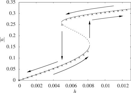
Figure 3: The hysteresis loop of the $\phi^{4}$ kink driven, parametrically, at the frequency close to its natural wobbling frequency. Continuous curves delineate stable and dashed curves unstable fixed points of the amplitude equation (32). Crosses represent numerical simulations of the full partial differential equation (30) with the same $\gamma$ and $\rho$. In the simulations, the driving strength $h$ was increased from zero in small steps and then turned back to zero as indicated by the arrows. This figure was generated using $\gamma=0.01$ and $\rho=-0.03$.

The damping term $\gamma\phi_{t}$ breaks the Lorentz invariance of the $\phi^{4}$ model (30). The kink travelling at the velocity $v$ is no longer equivalent to the kink at rest. Instead, according to (31), the traveling kink suffers deceleration — until $v$ becomes of order $|a|^{3}$. Thus, after an initial transient of the length $t\sim\gamma^{-1}$, the dynamics is governed by a single equation for the complex wobbling amplitude:

$${\dot{a}}+i\omega_{0}\rho a-\frac{i}{2}\omega_{0}\zeta|a|^{2}a=-\gamma a-i\frac{\pi}{8}\omega_{0}h.$$ (32)

Although the underlying partial differential equation (30) is driven parametrically, the forcing term in (32) is characteristic for the externally driven Schrödinger equations (see direct and references therein). The reason is that the oscillator that we are trying to pump energy to, is the kink’s internal mode rather than the kink itself. On the other hand, the leading part of the forcing term in the right-hand side of (30), $h\cos(\Omega t)\phi_{0}$, involves the kink ($\phi_{0}$) rather than the internal mode ($\phi_{1}$). As a result, the driver that was expected to affect a parameter of the oscillatory mode, acts as an external periodic force with regard to this mode.

The equation (32) has no attractors other than fixed points. Assume the damping coefficient $\gamma$ is fixed. When the detuning $\rho$ satisfies $\rho>\rho_{0}$, where $\rho_{0}=-1.14\gamma$, the dynamical system (32) has a single fixed point irrespectively of the value of $h$. The fixed point is stable and attracts all trajectories. If the detuning is chosen in the complementary domain $\rho<\rho_{0}$, the structure of the phase space depends on the value of $h$. Namely, there are two critical values $h_{+}$ and $h_{-}$, where $h_{+}<h_{-}$, such that when $h$ is smaller than $h_{+}$ or larger than $h_{-}$, the system’s phase portrait features a single fixed point — and this point is attractive. The inner region $h_{+}<h<h_{-}$ is characterised by two stable fixed points and exhibits hysteresis. (See Fig 3.) The values $h_{+}$ and $h_{-}$ are expressible through $\rho$ and $\gamma$ OB .

The memory function associated with the bistability and hysteresis of the parametrically driven wobbling kink, endows this structure with potential applications in electronic circuits, devices based on ferromagnetism or ferroelectricity, and charge-density wave materials.

6.2 Parametric driving at twice the natural wobbling frequency

The longest and widest Arnold tongue of the parametricaly driven harmonic oscillator corresponds to the subharmonic resonance where the driving frequency is close to twice the natural frequency of the oscillator. It is therefore interesting to examine this driving regime in the context of the wobbling kink. Would the $2:1$ frequency ratio sustain a larger wobbling amplitude than the $1:1$ regime considered in the previous subsection?

The driven equation in this case has the form

$$\frac{1}{2}\phi_{tt}-\frac{1}{2}\phi_{xx}-\phi+\phi^{3}=-\gamma\phi_{t}+h\cos(2\Omega t)\phi,$$ (33)

where, as in the previous subsection, we set

$$\Omega=\omega_{0}(1+\rho).$$

The scaling laws for the weak detuning and small driving amplitude are chosen as before:

$$\rho=\epsilon^{2}R,\quad\gamma=\epsilon^{2}\Gamma.$$

This time, however, it is convenient to choose a different scaling law for the small driving amplitude:

$$h=\epsilon^{2}H.$$

The resulting amplitude system is OB

$${\dot{a}}=-\gamma a-i\omega_{0}\left(\rho+\frac{v^{2}}{2}\right)a+\frac{i}{2}\omega_{0}\zeta|a|^{2}a-\frac{i}{2}\omega_{0}\sigma ha^{*}+O(|a|^{5}),$$

$${\dot{v}}=-2\gamma v+O(|a|^{5}).$$

Here the complex coefficient $\sigma=\sigma_{R}+i\sigma_{I}$ is given by an integral

$$\sigma=\int_{-\infty}^{\infty}\left[\frac{1}{2}\mathrm{sech}^{2}X_{0}\tanh^{2}X_{0}-6\mathrm{sech}^{2}X_{0}\tanh^{3}X_{0}f_{2}(X_{0})\right]dX_{0},$$ (34)

where $f_{2}$ consists of the second-harmonic radiation and a stationary standing wave — both induced by the driver:

$$f_{2}(X_{0})=-\frac{1}{12}f_{1}(X_{0})+\frac{1}{24}\tanh X_{0}(2\mathrm{sech}^{2}X_{0}-3).$$

In the above expression, the function $f_{1}$ is given by the equation (11). The real and imaginary parts of the integral (34) are found to be

$$\sigma_{R}=0.60,\quad\sigma_{I}=\frac{1}{12}\zeta_{I}=0.0039.$$

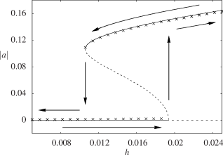
Figure 4: The hysteresis loop of the kink driven, parametrically, at the frequency close to twice its natural wobbling frequency. Continuous and dashed curves delineate stable and unstable fixed points of the amplitude equation (35) with $\gamma=0.005$ and $\rho=-0.005$. Crosses represent results of the numerical simulations of the equation (33) with the same $\gamma$ and $\rho$. The driving strength $h$ was increased from $0.005$ to $0.025$ in small steps and then turned back to $0.005$ as indicated by the arrows.

After a transient of the length $t\sim\gamma^{-1}$, the dynamics is governed by a two-dimensional dynamical system

$${\dot{a}}+i\omega_{0}\rho a-\frac{i}{2}\omega_{0}\zeta|a|^{2}a=-\gamma a-\frac{1}{2}i\omega_{0}\sigma ha^{*}.$$ (35)

Equation (35) is similar to the equation (32) from the previous section; the only difference between the two expressions is the type of the driver. Unlike equation (32), the amplitude equation (35) features the parametric forcing in its standard Schrödinger form (see e.g. parametric ).

The energy-transfer mechanism in the present case is different from the mechanism operating in the $1:1$ forcing regime. In the partial differential equation (33), the function $\cos(2\Omega t)$ in the product $h\cos(2\Omega t)(\phi_{0}+\epsilon\phi_{1}+...)$, acts as a parametric driver for the wobbling mode $\phi_{1}$. In addition, the “external force” $h\cos(2\Omega t)\phi_{0}$ excites a standing wave with the frequency $2\Omega$ and generates radiation at the same frequency. Both couple to the wobbling mode — parametrically, via the term $\epsilon^{3}\phi_{0}\phi_{1}\phi_{2}$ in the expansion of $\phi^{3}$. As a result, in the case of the equation (33) we have three concurrent mechanisms at work, and all three are of parametric nature. Combined, the three mechanisms produce the $ha^{*}$-term in the amplitude equation (35).

Turning to the analysis of the amplitude equation, we assume, first, that $\rho>\rho_{0}$, where $\rho_{0}=-0.031\gamma$. There is a critical value of the driving amplitude $h_{+}(\gamma,\rho)$ such that the dynamical system (35) has two stable fixed points $a_{1}$ and $-a_{1}$ in the region $h>h_{+}$ and a single stable fixed point $a=0$ in the complementary region $h<h_{+}$.

If the frequency detuning is taken to satisfy $\rho<\rho_{0}$, all trajectories flow to the origin for $h$ smaller than $h_{-}$ (where $h_{-}$ is another critical value expressible through $\gamma$ and $\rho$), and to one of the two nontrivial fixed points $\pm a_{1}$ for large $h$ ($h>h_{+}$). In the intermediate region $h_{-}<h<h_{+}$ the system shows a tristability between $a=0$ and the pair of points $a=\pm a_{1}$. See Fig 4.

6.3 External subharmonic driving

Proceeding to the analysis of the direct driving force, we start with the case where the driving frequency is approximately a half of the natural wobbling frequency of the kink QuinteroDirect :

$$\frac{1}{2}\phi_{tt}-\frac{1}{2}\phi_{xx}-\phi+\phi^{3}=-\gamma\phi_{t}+h\cos\left(\frac{\Omega}{2}t\right).$$ (36)

Here, as in the previous subsections, $\Omega=\omega_{0}(1+\rho)$. We keep our usual scaling laws for the small detuning $\rho=\epsilon^{2}R$ and damping coefficient $\gamma=\epsilon^{2}\Gamma$, but choose a fractional order of smallness for the driving amplitude: $h=\epsilon^{3/2}H$.

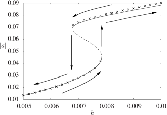
Figure 5: The hysteresis loop of the kink driven by an external subharmonic force. The continuous and dashed lines depict the stable and unstable fixed points of the dynamical system (37). Crosses result from the numerical simulations of the partial differential equation (36), with the same $\gamma$ and $\rho$. (In this plot, $\gamma=10^{-3}$ and $\rho=-2\times 10^{-3}$.) The driving strength $h$ is increased in small increments and then turned down. The dependence of $|a|$ on $h$ is similar to the one in Fig 3; yet the same driving strength sustains a much smaller wobbling amplitude than in Fig 3.

One amplitude equation is standard, ${\dot{v}}=-2\gamma v+O(|a|^{5})$. Once the velocity has become of order $|a|^{3}$, it drops out of the second equation which then acquires the form OB

$${\dot{a}}+i\omega_{0}\left(\rho+\frac{\lambda}{2}h^{2}\right)a-\frac{i}{2}\omega_{0}\zeta|a|^{2}a=-\gamma a+i\frac{60}{169}\pi\omega_{0}h^{2}.$$ (37)

Note that the term proportional to $\lambda$ is of higher order than all other terms in this equation. We had to include this forth-order correction to improve the agreement between the fixed points of the dynamical system (37) and results of simulation of the full partial differential equation (36). The fact that a higher-order term makes a significant contribution is due to its large coefficient: $\lambda=-7.47-1.68\,i$.

The equation (37) coincides with the equation (32) that we considered earlier, with $\rho$ replaced with $\rho^{\prime}=\rho+\lambda h^{2}/2$, $h$ with $h^{\prime}=\frac{480}{169}h^{2}$, and $a^{\prime}=-a$. Hence the dynamics of the $1:2$ externally driven wobbllng kink reproduce those of the kink driven by the $1:1$ parametric force.

As in that earlier system, the absence or presence of hysteresis in the dynamics depends on whether $\rho^{\prime}$ is above or below the critical value $\rho_{0}=-1.14\gamma$. If the difference $\rho^{\prime}-\rho_{0}$ is positive, all trajectories are attracted to a single fixed point. If, on the other hand, $\rho^{\prime}-\rho_{0}<0$, we have two stable fixed points for each $h^{\prime}$ in a finite interval $(h_{+},h_{-})$, where $h_{+}$ and $h_{-}$ are expressible through $\rho^{\prime}$ and $\gamma$. This bistability leads to the hysteretic phenomena similar to the one depicted in Fig 3. Outside the interval $(h_{+},h_{-})$, all trajectories flow to a single fixed point. See Fig 5.

The energy transfer mechanism associated with the $1:2$ external pumping deserves to be commented. It was suggested QuinteroDirect that the mechanism consists in the coupling of the wobbling to the translation mode. Our asymptotic expansion furnishes OB a different explanation though.

Expanding $\phi$ in powers of $\epsilon^{1/2}$,

$$\phi=\phi_{0}+\epsilon\phi_{1}+\epsilon^{3/2}\phi_{3/2}+\epsilon^{2}\phi_{2}+\epsilon^{5/2}\phi_{5/2}+\ldots,$$

we observe that the external driver excites an even-parity standing wave $\phi_{3/2}$ at its frequency $\Omega/2$. The standing wave undergoes frequency doubling and parity transmutation via the term $\epsilon^{3}\phi_{0}\phi_{3/2}^{2}$ in the expansion of $\phi^{3}$. It is this latter term that serves as an external driver for the wobbling mode. It has the resonant frequency $\Omega$ and its parity coincides with the parity of the mode.

This energy-pumping mechanism is a two-stage process and the resulting effective driving strength is proportional to $h^{2}$ rather than $h$. As a result, the external subharmonic driving sustains a much smaller wobbling amplitude than the harmonic parametric forcing. This conclusion is obvious if one compares the vertical scales in Fig 5 and Fig 3.

6.4 External harmonic driving

Driving the kink by an external periodic force with the wobbling frequency leads to the most interesting phenomenology. In this case the $\phi^{4}$ equation has the form QuinteroDirect

$$\frac{1}{2}\phi_{tt}-\frac{1}{2}\phi_{xx}-\phi+\phi^{3}=-\gamma\phi_{t}+h\cos(\Omega t),$$ (38)

where $\Omega=\omega_{0}(1+\rho)$. As in the previous three cases, we let $\rho=\epsilon^{2}R$ and $\gamma=\epsilon^{2}\Gamma$. Choosing a linear scaling for the driving amplitude, $h=\epsilon H$, and assuming that the velocity $v=\epsilon^{2}V$ (rather than $\epsilon V$ as before), we obtain the following system of two amplitude equations OB :

$${\dot{a}}+i\omega_{0}\left(\rho+\frac{\nu}{2}h^{2}\right)a-\frac{i}{2}\omega_{0}\zeta|a|^{2}a=-\gamma a+\frac{3\pi}{4}vh-\frac{i}{2}\omega_{0}\mu h^{2}a^{*}+O(|a|^{5}),$$ (39)

$${\dot{v}}=-2\gamma v+\frac{3}{2}h\left[\frac{\pi}{2}\omega_{0}\left(\omega_{0}\rho+i\gamma\right)-\eta|a|^{2}-\chi h^{2}\right]a+c.c.+O(|a|^{5}).$$ (40)

Here $\nu$, $\mu$, $\eta$, and $\chi$ are numerical coefficients:

$$\nu=4.16-0.33\,i,\quad\mu=1.02+0.16\,i,$$

$$\eta=-2.00-0.38\,i,\quad\chi=-12.21-0.57\,i.$$

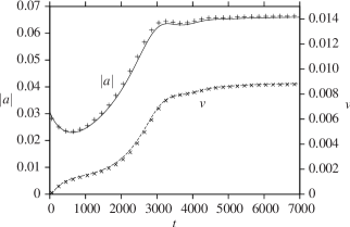
Figure 6: The wobbling kink set in motion by the harmonic external force. The curves were obtained by solving the amplitude equations (39)-(40). The crosses represent numerical simulations of the partial differential equation (38) with the corresponding initial conditions. In this plot, $h=0.012$, $\gamma=0.001$ and $\rho=0$.

According to the equation (40), the velocity does not drop out of the system; instead, it plays an important role in the dynamics. Unlike all types of driving that we considered so far, the harmonic external driving can sustain the translational motion of the kink. Fig 6 shows an example of the kink accelerated by the 1:1 direct driving force which simultaneously excites the wobbling OB .

When $h$ is small, the fixed point at $a=v=0$ is the only attractor in the system. As $h$ is increased while keeping the parameters $\gamma$ and $\rho$ constant, a pair of fixed points $(a,v)$ and $(-a,-v)$, with nonzero $a$ and $v$, bifurcates from the trivial fixed point (see Fig.7).

As the driving strength approaches some critical value $h_{\rm c}$, the $|a|$- and $v$-component of these points grow to infinity. No stable fixed points exist in the parameter region beyond $h_{\rm c}$. In that region, all trajectories escape to infinity: $|a(t)|\to\infty,v(t)\to\infty$ as $t\to\infty$. The critical value $h_{\rm c}$ can be determined assuming that the growth is self-similar, that is, that $v$ grows as a power of $|a|$. This assumption leads to a simple exponential asymptote $e^{\mathfrak{r}t}$ for $|a(t)|$, with the growth rate OB

$${\mathfrak{r}}=-\frac{2}{3}\gamma-\frac{3\pi i}{4\omega_{0}}\,\frac{\eta\zeta^{*}-\zeta\eta^{*}}{|\zeta|^{2}}h^{2}.$$

Setting $\mathfrak{r}=0$ gives

$$h_{\rm c}=0.65\gamma^{1/2}.$$ (41)

In the vicinity of the critical value (41) our smallness assumptions about $|a|$ and $v$ are no longer met and the amplitude system (39)-(40) is no longer valid. The simulations of the full partial differential equation (38) with $h$ just below and just above $h_{\rm c}$, reveal that the kink does settle to the wobbling with finite amplitude here. This is accompanied by its motion with constant velocity. However, the observed value of the wobbling amplitude is $O(\gamma^{1/3})$ rather than $O(\gamma^{1/2})$ as we assumed in the derivation of (39)-(40), and the measured value of the kink velocity is $O(\gamma^{1/3})$ rather than $O(\gamma)$. This change of scaling accounts for the breakdown of our asymptotic expansion in the vicinity of $h_{\rm c}$.

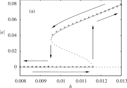
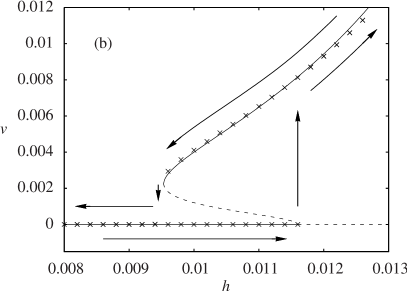
Figure 7: The hysteresis loop of the wobbling kink driven by an external harmonic force. The continuous and dashed curves delineate the stable and unstable fixed points of the amplitude equations (39)-(40), with $\gamma=10^{-3}$ and $\rho=-10^{-4}$. The crosses indicate results of the numerical simulations of the partial differential equation (38) with the same $\gamma$ and $\rho$. The driving amplitude is increased from $h=8\times 10^{-3}$ to $13\times 10^{-3}$ in small steps and then turned back to $8\times 10^{-3}$.

Since the spatially uniform (even) driving force has an opposite parity to that of the (odd) wobbling mode, the energy transfer mechanism has to be indirect here. In fact there are two mechanisms at work, both involving a standing wave with the frequency $\Omega$ excited by the external driver. In the first mechanism, the square of this wave, its zeroth and second harmonics as well as the radiation excited by this wave, couple, parametrically, to the wobbling mode. The second mechanism exploits the fact that when the kink moves relative to the standing wave, the wobbling mode acquires an even-parity component. It is this part of the mode that couples — directly — to the standing wave.

7 Concluding remarks

The first objective of this article was to review the multiscale singular perturbation expansion for the wobbling kink of the $\phi^{4}$ model. The advantage of this approach over the Lindstedt method, is that it takes into account the existence of a hierarchy of space and time scales in the system. In particular, the multiscale expansion provides a consistent treatment of the long-range radiation from the oscillating kink.

The central outcome of the asymptotic analysis is the equation (17) for the amplitude of the wobbling mode. The nonlinear frequency shift and the lifetime of the wobbling mode are straightforward from this amplitude equation. We have identified the main factor ensuring its longevity. This is a small amplitude of radiation due to the significant difference between the wavelength of the radiation and the characteristic width of the wobbling kink.

The second part of this brief review (section 6) concerned ways of sustaining the wobbling of the kink indefinitely. We discussed four resonant frequency regimes, namely the $1:1$ and $2:1$ parametric driving, and $1:2$ and $1:1$ external forcing.

It is instructive to compare the amplitude of the stationary wobbling mode sustained by these four types of resonance. For the given driving strength $h$, the harmonic ($1:1$) parametric driver ensures the strongest possible response. In this case the amplitude of the stationary kink oscillations is of the order of $h^{1/3}$. The “standard” parametric resonance, where the driving frequency is chosen to be near twice the natural wobbling frequency of the kink, is second strongest. In this case the wobbling amplitude is of the order of $h^{1/2}$. The direct driving at half the wobbling frequency produces oscillations with the amplitude $a\sim h^{2/3}$. Finally, the harmonic ($1:1$) direct resonance is the weakest of the four responses considered. In this case, the amplitude of the forced oscillations of the kink is $a\sim h$.

Another resonance characteristic worth comparing, is the width of the “Arnold tongue” — the domain on the $(\Omega,h)$ parameter plane where the driver sustains stable stationary wobbling of the kink. The $1:1$ parametric driver produces the widest tongue; in this case the resonant region is bounded by the curve $h\sim\rho^{3/2}$. The “standard” ($2:1$) parametric resonance is the second widest, bounded by the curve $h\sim\rho$. The Arnold tongue for the external driving force with the frequency $\Omega/2$, is bounded by $h\sim\rho^{3/4}$. Finally, the harmonic direct resonance is the narrowest of the four, with the boundary curve $h\sim\rho^{1/2}$.

Our comparison would be incomplete without noting that neither the harmonic parametric driver nor the $\Omega/2$ direct driving force have to overcome any thresholds in order to sustain stationary wobbling with a nonzero amplitude. In contrast, the subharmonic ($2:1$) parametric and harmonic ($1:1$) direct resonances occur only if the driving amplitude exceeds a certain threshold value.

Thus, the harmonic external driving emerges as the least efficient way of sustaining the steady wobbling of the kink. Out of the four driving techniques considered in section 6, it produces the weakest response, requires the finest tuning of the driving frequency while the corresponding driving strength has to overcome a threshold set by the dissipation. Although these factors are indeed disadvantageous, the harmonic external driving gives rise to an interesting “rack and pinion” mechanism that converts the energy of external oscillation to the translational motion of the kink (Fig 8). This mechanism may prove useful for the control of solitons with internal modes in other systems.

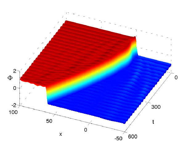
Figure 8: A kink accelerates from rest as its wobbling mode couples to the standing wave excited by the resonant harmonic force. The figure is produced by numerical simulation of equation (38) with $\gamma=10^{-3}$, $\rho=10^{-2}$, and $h=4\times 10^{-2}$. The initial conditions are $\phi_{t}=0$ and $\phi=\tanh x+2a\tanh x\,\mathrm{sech}\,x$ with $a=0.3$.

8 Epilogue

This brief review is a tribute to Boris Getmanov, a musician and nonlinear scientist. A whole generation of former school kids still recalls gyrating to his band’s boogie grooves while those with a taste for integrable systems remember Getmanov’s discovery of the complex sine-Gordon BG1 . (Incidentally, that discovery was only possible due to his numerical experimentation with the $\phi^{4}$ model.) While Bob’s piano is no longer heard at Dubna parties, the $\phi^{4}$ and sine-Gordon equations are still around, alluring their new insomniacs and artists.

References

- (1) B S Getmanov, JETP Letters 24 291 (1976)
- (2) D K Campbell, J F Schonfeld, and C A Wingate, Physica D 9 1 (1983); M Peyrard and D K Campbell, Physica D 9 33 (1983); D K Campbell and M Peyrard, Physica D 18 47 (1986); D K Campbell, M Peyrard and P Sodano, Physica D 19 165 (1986); T I Belova and A E Kudryavtsev, Physica D 32 18 (1988); P Anninos, S Oliveira, R A Matzner, Phys Rev D 44 1147 (1991); R H Goodman and R Haberman, Phys Rev Lett 98 104103 (2007); I Takyi and H Weigel, Phys Rev D 94 085008 (2016)
- (3) T I Belova, JETP 89 587 (1996)
- (4) T I Belova and A E Kudryavtsev, Physics-Uspekhi 40 359 (1997)
- (5) Z Fei, Y S Kivshar and L Vázquez, Phys Rev A 46 5214 (1992)
- (6) N S Manton and H Merabet, Nonlinearity 10 3 (1997)
- (7) T Romańczukiewicz, Acta Phys Polonica B 36 3877 (2005); T Romańczukiewicz, J Phys A: Math Theor 39 3479 (2006)
- (8) A L Sukstanskii and K I Primak, Phys Rev Lett 75 3029 (1995)
- (9) O F Oxtoby and I V Barashenkov, Phys Rev E 80 026609 (2009)
- (10) Z Fei, V V Konotop, M Peyrard, and L Vázquez, Phys Rev E 48 548 (1993)
- (11) B A Malomed, J. Phys. A: Math. Gen. 25 755 (1992)
- (12) N A Voronov, I Y Kobzarev, and N B Konyukhova, JETP Lett 22 290 (1975); I L Bogolyubskii and V G Makhankov, JETP Lett 24 12 (1976); N A Voronov and I Y Kobzarev, JETP Lett 24 532 (1976); I L Bogolyubskii and V G Makhankov, JETP Lett 25 107 (1977); T I Belova, N A Voronov, I Yu Kobzarev, and N B Konyukhova, Sov Phys JETP 46 846 (1977)
- (13) M J Rice, A R Bishop, J A Krumhansl, and S E Trullinger, Phys Rev Lett 36, 432 (1976); M J Rice, Phys Lett A 71 152 (1979); M J Rice and J Timonen, Phys Lett A 73 368 (1979)
- (14) M J Rice and E J Mele, Solid State Commun 35 487 (1980)
- (15) M J Rice, Phys Rev B 28 3587 (1983)
- (16) H Segur, J Math Phys 24 1439 (1983)
- (17) M Ślusarczyk, Acta Phys Polonica B 31 617 (2000)
- (18) R Pełka, Acta Phys Polonica B 28 1981 (1997)
- (19) T Romańczukiewicz, Acta Phys Polonica B 35 523 (2004)
- (20) O M Kiselev, Russian J of Mathematical Physics 5 29 (1994)
- (21) I V Barashenkov and O F Oxtoby, Phys Rev E 80 026608 (2009)
- (22) M Borromeo, F Marchesoni, Chaos 15 026110 (2005)
- (23) L Morales-Molina, F Mertens, A Sánchez, Phys Rev E 72 016612 (2005)
- (24) L Morales-Molina, N Quintero, A Sánchez, F Mertens, Chaos 16 013117 (2006)
- (25) N Quintero, A Sánchez, and F Mertens, Phys Rev Lett 84 871 (2000); N Quintero, A Sánchez, and F Mertens, Phys Rev E 62 5695 (2000)
- (26) N Quintero, A Sánchez, and F Mertens, Phys Rev E 64 046601 (2001)
- (27) I V Barashenkov and E V Zemlyanaya, Physica D 132 363 (1999); I V Barashenkov and E V Zemlyanaya, J Phys A: Math Theor 44 465211 (2011)
- (28) I V Barashenkov, E V Zemlyanaya and M Bär, Phys Rev E 64 016603 (2001); I V Barashenkov and S R Woodford, Phys Rev E 71 026613 (2005); I V Barashenkov, S R Woodford and E V Zemlyanaya, Phys Rev E 75 026604 (2007); I V Barashenkov and E V Zemlyanaya, Phys Rev E 83 056610 (2011)
- (29) B S Getmanov, JETP Letters 25 119 (1977); B S Getmanov, Theor Math Phys 38 124 (1977); B S Getmanov, Theor Math Phys 48 572 (1981)