Machine Learning Phase Transition: An Iterative Proposal

Abstract

We propose an iterative proposal to estimate critical points for statistical models based on configurations by combing machine-learning tools. Firstly, phase scenarios and preliminary boundaries of phases are obtained by dimensionality-reduction techniques. Besides, this step not only provides labelled samples for the subsequent step but also is necessary for its application to novel statistical models. Secondly, making use of these samples as training set, neural networks are employed to assign labels to those samples between the phase boundaries in an iterative manner. Newly labelled samples would be put in the training set used in subsequent training and the phase boundaries would be updated as well. The average of the phase boundaries is expected to converge to the critical temperature in this proposal. In concrete examples, we implement this proposal to estimate the critical temperatures for two q-state Potts models with continuous and first order phase transitions. Linear and manifold dimensionality-reduction techniques are employed in the first step. Both a convolutional neural network and a bidirectional recurrent neural network with long short-term memory units perform well for two Potts models in the second step. The convergent behaviors of the estimations reflect the types of phase transitions. And the results indicate that our proposal may be used to explore phase transitions for new general statistical models.

I Introduction

Machine learning is an advancement in computer science and technology adept at processing big data intelligently and has been applied to various applications in life such as image recognition, natural language processing and so on Science349255 ; Nature521436 ; HBTNN3361 ; Goodfellowbook . In the field of theoretical condensed matter physics, the exponentially large Hilbert space usually makes calculations formidable for conventional approaches. With the advancing of computation power and the amelioration of algorithms, machine learning provides novel avenues to distill critical characteristics for configurations of statistical models and shows its talents in the context of classifying phases for condensed matter NP13431 ; NP13435 ; PRX7031038 ; PRL118216401 ; PRB96245119 ; PRL120066401 ; PRB94195105 ; PRB96195138 ; PRE95062122 ; PRE96022140 ; PRB96144432 .

In machine learning, architectures usually deal with massive samples which can be represented by points in feature spaces. Statistical characteristics can be analyzed by studying the distribution scenarios or patterns of such points, merely efficiency of analysis may be discounted due to redundant information and noise. Nevertheless, dealing with essential characteristic patterns would be conducive to improve the efficiency. The linear and manifold dimensionality-reduction techniques are frequently adopted in unsupervised machine-learning tasks to decrease redundant information and compress data PM2559 ; IJPCA ; NN11 . Due to their ability to reveal characteristic patterns for data sets, such techniques have been employed to investigate phase transitions and order parameters from the configurations of the classical Ising model PRB94195105 ; PRE95062122 ; PRB96144432 ; PRB96195138 ; PRE96022140 . Such tools are suitable for representing data with essential information maintained as more as possible in a space with lower dimensionality without using supervised labels.

Different to unsupervised treatment, neural networks trained by samples with supervised labels are adept at classification tasks. During training, the parameters of a neural network would be updated in order to minimize a cost or loss function constructed by the output and supervised label. Such supervised learning tools have been employed to investigate Ising model NP13431 ; NP13435 , study strongly correlated fermions PRX7031038 ; PRB94245129 , and explore the fermion-sign problem SR78823 . Nontrivial topological states can also be learned by artificial neural networks. For example, by introducing quantum loop topography, a fully connected neural network can be trained to distinguish the Chern insulator and the fractional Chern insulator from trivial insulators PRL118216401 . The phase boundary between topological and trivial phases can also be identified by a feed-forward neural network PRB96245119 . Neural network can also be trained to learn the discrete version of the winding-number formula from a set of Hamiltonians of topological band insulators PRL120066401 . The map between variational renormalization group and restricted Boltzmann machines has also been studied arxiv14103831 . Quantum inspired tensor networks have been applied to multi-class supervised learning tasks and demonstrated by using matrix product states to parameterize models ANIP294799 . An artificial neural network trained on entanglement spectra of individual states of a many-body quantum system can be used to determine the transition between a many-body localized and a thermalized region PRB95245134 . The classification power of shallow fully connected and convolutional neural networks are examined by Ising model, concentrating on the effect of extended domain wall configurations PRB97174435 . The generalizing and interpretability properties of machine-learning algorithms have been demonstrated by inferring the phase diagram for a liquid-gas transition arxiv180702468 . These works indicate the power of neural networks in extracting the characteristics of the physical configurations.

As the works mentioned above, unsupervised learning techniques can be applied to cluster physical objects in terms of the distributions in feature space. Supervised learning are employed based on the extracting ability of neural networks for physical samples. In this work, we propose an iterative proposal combing unsupervised learning techniques and supervised machine-learning architectures to estimate critical temperatures for statistical models only using their configurations with temperatures. Firstly, dimensionality-reduction techniques are employed as unsupervised learning tools to obtain phase scenarios versus temperature by using the configurations (samples). Since no knowledge about phase transition is used, this is a necessary step for estimating critical points. It provides the scenario of the configurations in a range of temperature and preliminary phase boundaries. Meanwhile, initial labels for samples are obtained which would be used to train the neural networks subsequently. This step is also necessary for its application for new statistical models. Secondly, training the neural networks until they learn the characters of the existed samples, we use it to distinguish the samples with temperatures between the phase boundaries. Once the samples were recognized by the trained networks with high accuracy, they would be assigned the corresponding label and added into the training set to be used in subsequent training. Meanwhile, the phase boundaries would be updated by the temperatures of the last labelled samples. Without extra knowledge about scaling behavior is used, we set the average value of the phase boundaries as the estimation for critical points. Iterating the procedure of recognizing and updating above, the estimation for critical points is expected to converge to the critical temperatures. Q-state Potts models provide a testing ground for various methods in the study of critical point theory RMP54235 ; PCPS48106 . We demonstrate this proposal by two q-state Potts models with continuous and first order phase transitions, respectively.

Following in Sec. II, we describe the iterative proposal of sequentially combing dimensionality-reduction techniques and neural networks to estimate critical points. In Sec. III, we employ this proposal to estimate the critical points for two q-state Potts models with continuous and first order phase transitions and analyze the results. Finally, we summarize in Sec. IV.

II The Iterative Proposal

There are two sequential steps in this proposal. The first one plays a necessary role in providing preliminary phase boundaries and supervised labels used in the second step. The details are listed in the following.

II.1 Step-1: Dimensionality-reduction pretreatment

This proposal starts from raw configurations of statistical models without extra knowledge about phase transitions. The configurations can be represented by points distributed in a high dimensionality feature space with cluster behaviors related to phases. It is a necessary step to obtain preliminary phase scenarios and phase boundaries in this proposal. However high dimensionality usually makes it burdensome to analyze statistical models. Thus it is desirable to employ a simpler or more accessible representation which maintains essential information of the distributions as much as possible. Dimensionality-reduction techniques offer such tools to extract salient characteristics for distributions PM2559 ; IJPCA ; NN11 . Scenarios of phases can be reflected by the distribution behaviors of the projected points in a lower dimensionality space. The phases can be used as supervised labels for the configurations in supervised machine learning. The initial phase boundaries which confine the critical temperature are identified preliminarily. This pretreatment not only provides essential cornerstone for the subsequent step but also is indispensable for its application for unexplored statistical models when only raw configurations with temperatures are provided.

In this work we would employ singular value decomposition and multidimensional scaling which can be used in linear and manifold dimensionality-reduction tasks to do the unsupervised pretreament in the first step. However the choices of unsupervised techniques in this step are not limited to particular ones but any one which can be used to handle unsupervised clustering tasks may be a candidate. For example, uniform manifold approximation and projection which is based in Riemannian geometry and algebraic topology can also act as the unsupervised module here arxiv180702468 ; arxiv180203426 ; Isometric mapping algorithm represents the original data set on a quasi-isometric, low-dimensional space by preserving the geodesic distances between points on a neighborhood graph. This algorithm can also play the role above Science2902319 ; Besides, locally linear embedding which is used in manifold learning to obtain low-dimensional, neighborhood-preserved projections for high dimensional data sets can also be a candidate in this step LLE . These alternatives give this proposal generalization to be applied to new statistical models in term of distributions.

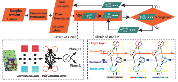
Figure 1: The sketch of this proposal to estimate critical temperatures. The critical structure of the convolutional neural network (CNN) and the bidirectional recurrent neural network with long short-term memory units (BLSTM) are shown. The CNN deals with the batches of configurations. Whereas configurations within the batches are split into rows as input denoted by $r$ when the BLSTM is employed.

Due to thermal fluctuations and information loss in the dimensionality-reduction treatment, those configurations between the phase boundaries would not be easily distinguished in the vicinity of critical points in this step. Benefiting from the pattern-extraction capability of neural networks, in the subsequent step II.2, we give the procedure employing such supervised learning architectures to estimate critical temperatures for statistical models further based on the results of Step-1.

II.2 Step-2: Estimating critical temperature iteratively

According to the results of Step-1, the critical point locates within the temperature interval where the labels of those samples have not been determined. In the following, we employ neural networks usually used in supervised learning tasks to estimate the critical temperatures for statistical models more accurately in an iterative way. Although we consider the situation that two phases are distinguished in Step-1, phase scenarios with more than two phases can be analyzed in segments with two phases. The workflow of this proposal is illustrated in Fig. 1. The details for the second step are listed below.

$Step_{1}$: $T_{low\leavevmode\nobreak\ boundary}$, $T_{high\leavevmode\nobreak\ boundary}$ and $T_{m}=(T_{low\leavevmode\nobreak\ boundary}+T_{high\leavevmode\nobreak\ boundary})/2$ are used to denote the temporal low-temperature-phase boundary, high-temperature-phase boundary, and the average for the boundaries (estimation for critical temperature $T_{c}$), respectively. Taking the samples labelled in the first step II.1 as preliminary training set, a neural network is trained until it can distinguish the whole training set with accuracy larger than a high threshold $S_{1t}$ within the number of $N_{1t}$ training batches used in training;

$Step_{2}$: If $Step_{1}$ is fulfilled, we use the trained neural network to recognize the samples at temperature $T_{m}$. If they are judged to be in ‘low-temperature phase (high-temperature phase)’ according to a criterion $\mathcal{C}_{m}$, we further judge those at temperature $T_{mm}=(T_{low\leavevmode\nobreak\ boundary}+T_{m})/2$ (or $T_{mm}=(T_{high\leavevmode\nobreak\ boundary}+T_{m})/2$) according to a criterion $\mathcal{C}_{mm}$ by the same trained neural network; Else, if $Step_{1}$ is not fulfilled, we purge the newly added samples from the training set in the last iteration and roll $T_{mm}$ back to the last value to continue the recognition process from $Step_{1}$;

$Step_{3}$: If samples at $T_{m}$ are judged to be in ‘low-temperature phase (high-temperature phase)’ and those at temperature $T_{mm}$ are also judged to be in ‘low-temperature phase (high-temperature phase)’, we assign the label to the samples at $T_{mm}$ as ‘low-temperature-phase label (high-temperature-phase label)’ and add the newly labelled samples into the training set, to be used in following iterations. Meanwhile we update $T_{low\leavevmode\nobreak\ boundary}=T_{mm}$ (or $T_{high\leavevmode\nobreak\ boundary}=T_{mm}$); Else, we update $T_{mm}=(T_{low\leavevmode\nobreak\ boundary}+T_{mm})/2$ (or $T_{mm}=(T_{high\leavevmode\nobreak\ boundary}+T_{mm})/2$) and carry out the procedure in this step until the samples at $T_{mm}$ are assigned a label with the criterion $\mathcal{C}_{mm}$. Then we turn to $Step_{1}$ to begin the next recognition iterations.

Indeed, this proposal gives an iterative way to assign labels with high accuracy from margins towards center. When phase boundaries approach $T_{c}$, thermal fluctuations make the characteristics contained in the samples become harder to be learned by the neural networks with high accuracy. Even so, the newly added samples with labels enrich the training set and benefit the neural networks learning characteristics. In $Step_{1}$, the threshold of recognition $S_{1t}$ is necessary to be set large and $N_{1t}$ is used to avoid overfitting. The criteria $\mathcal{C}_{m}$ and $\mathcal{C}_{mm}$ have bearing on assigning labels and we give the concrete forms in the concrete examples following.

Compared to the dimensionality-reduction pretreatment in the first step II.1, the function of the neural networks is more critical in terms of the precision of estimation. However the neural networks work based on the results of Step-1.

III Application to q-state Potts models

Now we turn to implement the proposal above to estimate the critical temperatures for two q-state Potts models on squire lattice with continuous and first order phase transitions respectively RMP54235 ; PCPS48106 .

III.1 Q-state Potts models

Q-state Potts models are generalizations of Ising model with rich contents and offer agents to study ferromagnet and certain other physics of solid states RMP54235 ; PCPS48106 . The general Hamiltonian for such models reads:

$$\begin{aligned} H=-J\sum_{\{i,j\}}\delta_{\sigma_{i},\sigma_{j}},\end{aligned}$$ (1)

where the coupling $J$ between nearest-neighbor spins is set as the energy unit in this work. $\delta_{\sigma_{i},\sigma_{j}}$ is the Kronecker delta function with regard to the variables $\sigma_{i}$ and $\sigma_{j}$ which take one of $q=(0,...,q-1)$ values with equal probabilities on each lattice site. A nearest-neighbor pair of same spins carries an unity energy and others are zero. While $q=2$, the Ising model is recovered in two dimensional case ZP31253 ; PR65117 . These models posses self-duality points at temperature $T_{c}$ given by $e^{1/k_{B}T_{c}}=1+\sqrt{q}$ RMP54235 . In two-dimensional case, continuous phase transitions occur at $T_{c}=1/\log(1+\sqrt{q})$ when $q\leq 4$, and first order phase transitions occur at this temperature when $q>4$ JPC6L445 ; PRSLSA358535 ; RMP54235 with Boltzmann constant $k_{B}=1$. In this work, only such spin configurations generated by Monte Carlo method would be used to estimate the critical temperatures JASA44335 ; RPP60487 ; MCBook . These models offer benchmarks to check the performance of our proposal.

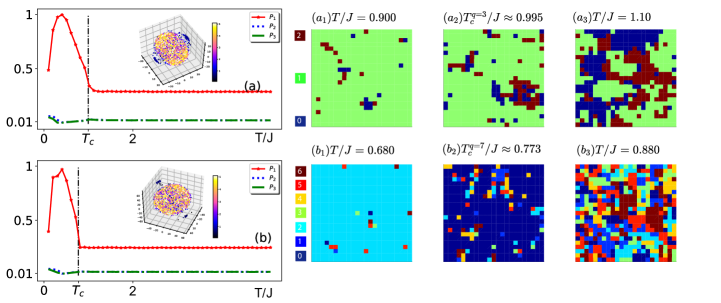
Figure 2: (a) the three leading normalized singular values ($P_{1}$, $P_{2}$ and $P_{3}$) as a function of temperature for 3-state Potts model with the result of Metric-MDS in the inset as describe in section III.2.1. The leading singular values at each temperature are calculated by a vertical stack of 40 flattened configurations . (b) the results of SVD and Metric-MDS for 7-state Potts model. The averages of the stacks have not been subtracted. This results to the bias in SVD but does not hamper the usage of this technique to reveal the phase transitions. The temperatures of the samples are mapped to the color of the projected dots. $(a_{i})$ (i=1,2,3) list three configurations for 3-state Potts model at different temperatures and $(b_{i})$ (i=1,2,3) list those for 7-state Potts model. The codes are given in the supplementary material SpMl .

Starting from the results of the first step II.1, we would employ a convolutional neural network (CNN) and a bidirectional recurrent neural network with long short-term memory units (BLSTM) to estimate the critical points for two q-state Potts models with different kinds of phase transitionsScience349255 ; Nature521436 ; HBTNN3361 ; Goodfellowbook ; PCPS48106 ; RMP54235 .

III.2 Dimensionality-reduction techniques

III.2.1 Singular value decomposition

According to section II, firstly, we give a brief introduction to a technique used in linear dimensionality-reduction: singular value decomposition (SVD) and one of manifold learning techniques: multidimensional scaling (MDS).

SVD is the core of principal component analysis to represent the original data in a lower dimensionality space where significant characteristics of statistical distributions are preserved IJPCA ; NN11 . While SVD reads $V=UZW^{T}$, the singular values are the diagonal elements of $Z$ usually normalized by dividing their summation and arranged in descending order  IJPCA ; NN11 . In this proposal $V$ is a vertical stack of flattened configurations in the form: $\mathbf{S}^{T}=(s_{11},...,s_{ij},...,s_{LL})^{T}$ with $s_{ij}$ denoting the spin value at site $(i,j)$ at temperature $T$. The original data are represented in a coordinate space where the covariance matrix is diagonalized by SVD. Since larger singular values together with the corresponding singular vectors carry more essential information of the original matrix, we will employ the three leading singular values to do the task for the first step II.1.

III.2.2 Multidimensional scaling

No information is offered to indicate that linear dimensionality-reduction treatment can reflect the phase scenarios comprehensively here. For generality, we further employ MDS which is manifold learning technique to construct a lower dimensionality representation for the original data sets. There are mainly two kinds of MDS: one is called Non-Metric Multidimensional Scaling which preserves the ranks of the distances between the samples SAGE ; CMS ; Borgbook ; RDS133 ; The other one is called Metric Multidimensional Scaling (Metric-MDS) which tries to reproduce the original Euclidean distances between pairs of points as well as possible in a lower dimensionality space and would be employed in this work. This method attempts to visualize the degree of similarities or dissimilarities for the investigated samples SAGE ; CMS ; Borgbook ; RDS133 .

Several loss functions can be constructed and optimized in Metric-MDS SAGE ; CMS ; Borgbook ; RDS133 . For example, supposing a distance matrix ${\textstyle D^{\prime}=\{d_{ij}^{\prime}\}}$ with ${\textstyle d_{ij}^{\prime}=\sum_{k=1}^{p}{||x_{ki}^{\prime}-x_{kj}^{\prime}||}}$ in a reduced $p$-dimensionality space to approximate the Euclidean distance matrix ${\textstyle D=\{d_{ij}\}}$ of the pair-wise distances between samples $x_{i}$ and $x_{j}$ in the original space, a candidate loss function $Stress=\sum_{i,j}(\frac{||d_{ij}^{\prime}-d_{ij}||^{2}}{\sum_{i,j}d^{\prime 2}_{ij}})^{1/2}$ can be minimized based on the differences between projected and original distances. Given the matrix ${\textstyle D}$ for the original data set, a simple procedure for Metric-MDS follows:

$S_{1}$: Appoint an arbitrary set of coordinates for projected points in a dimensionality reduced space with dimensionality $p$ ($p<4$, since distributions in spaces with dimensionality larger than 3 are difficult to be visualized);

$S_{2}$: Compute Euclidean distances among all pairs of projected points to form the matrix ${\textstyle D^{\prime}=\{d_{ij}^{\prime}\}}$;

$S_{3}$: Evaluate loss function $Stress$ based on ${\textstyle D}^{\prime}$ and ${\textstyle D}$;

$S_{4}$: Adjust coordinates $\{x_{k1}^{\prime},\leavevmode\nobreak\ x_{k2}^{\prime},\leavevmode\nobreak\ ...,\leavevmode\nobreak\ x_{kN}^{\prime}\}$ to minimize $Stress$;

$S_{5}$: Repeat the steps from $S_{2}$ to $S_{4}$ above until $Stress$ ceases decreasing.

$Stress$ is usually minimized by SMACOF (shorthand for Scaling by MAjorizing a COmplicated Function) SAGE ; CMS ; Borgbook ; RDS133 . And it decreases $Stress$ as a convex-optimization problem. Dimensionality-reduction treatment mentioned can be finished by Scikit-learn Sklearn

III.3 Neural networks

CNN and BLSTM are both artificial neural networks (ANN) HBTNN3361 ; Goodfellowbook ; NN11 ; SSP1361 . In general classification tasks, the input $X_{i}$ (usually being a tensor fed into ANN and $i$ denotes classes) with the supervised label $Y_{i}$ would be used to train the ANN. $Y_{i}$ is usually treated as a distribution with $i$th component being one and others zero, in order to construct a cost function measuring the difference between the output of the ANN and the supervised labels. The parameters of ANN would be updated by algorithms to reduce the cost function. Convolutional operation plays an important role in CNN in company with nonlinear activation functions and some regulative operations. This operation extracts correlations in the samples in a region covered by convolutional filters with weights and biases to be updated. However in classification tasks, the rows (columns) in samples can be treated as ordered ‘elements’ by recurrent neural networks. Thus the recurrent neural networks learn the samples in a global manner and long correlations can be extracted especially with LSTM units. In this proposal, once the samples with new temperatures between the phase boundaries are mapped into a certain category (phase) by the trained neural networks with high accuracy, they would be assigned the corresponding label and added into the training set. Thus along with the iterative process, the neural networks would be acquainted with the samples more and more accurately. To get an insight of the mapping process, an example of inputs, a batch of weights in the neural networks and the outputs are shown in the Appendix APPENDIX. Different kinds of abstract characters would be extracted during training with the purpose to minimize the cost functions.

III.3.1 The convolutional neural network

In terms of feature-map mechanisms of neural networks to extract characteristics of images, the configurations with similar patterns can be mapped into the same category with high accuracyNature521436 ; HBTNN3361 ; Goodfellowbook ; ANIPS1097 . Firstly, we elaborate the workflow of the CNN to learn the phases: Samples at $T/J$ $\rightarrow$ Convolutional operation-1 $\rightarrow$ ELU activation operation $\rightarrow$ Max pooling $\rightarrow$ Convolutional operation-2 $\rightarrow$ ELU activation operation $\rightarrow$ Max pooling $\rightarrow$ Fully connected operation-1 $\rightarrow$ ELU activation operation $\rightarrow$ Dropout operation $\rightarrow$ Fully connected operation-2 $\rightarrow$ Calculate loss by processing cross-entropy cost function after Softmax operation $\rightarrow$ Employ Adam algorithm to minimize the cost function.

Then we give a brief instruction to the operations in the CNN above as in Fig.1. The critical operation is finished in convolutional layers through multiplying the pixels in a window of an input sample by the corresponding pixels in convolutional kernels cover the window, and biases are usually added. The kernels slide across the samples until all the pixels are visited to finish one time of convolutional map. The weights and the biases are shared during this operation. This reduces the amount of parameters. An example of convolutional operation is shown in the appendix APPENDIX. To make the network be capable of extracting more kinds of features, several kernels are usually adopted. To extract more complex and abstract characteristics and improve the capability of recognition, deeper neural networks are recommendable candidates.

After the convolutional operation, Exponential Linear Units (ELU):

$$ELU(x)=\left\{\begin{array}[]{ll}x,\leavevmode\nobreak\ \leavevmode\nobreak\ \leavevmode\nobreak\ \leavevmode\nobreak\ \leavevmode\nobreak\ \leavevmode\nobreak\ \leavevmode\nobreak\ x>0,\\ e^{x}-1,\leavevmode\nobreak\ x<0,\\ \end{array}\right.$$ (4)

would be employed as the activation function in this work ELU . Compared to the prevalent activation function Rectified Linear Unit (ReLU) P27ICML807 , ELU has negative values which pushes the mean of activation closer to zero. This decreases the bias-shift effect and benefits machine learning with lower computational complexity ELU . Besides, the novel activation function: Swish performs better than ReLU in a number of scenes, and may be intriguing to be investigated in comparison with ReLU and ELU arxiv171005941 . Max pooling operation converts high resolution matrix to lower resolution counterparts by outputting the maximum value in a sampling window. This operation reduces the amount of computation and preserves the essential information in a compact form. It not only makes feature detection more robust to scale and noise but also is beneficial to avoid overfitting, merely some information lost. Other versions of pooling, such as Average pooling or L2-norm pooling may also perform well arxiv12070580 .

Fully connected layers can be adopted to purify the information for next classification operations. Dropout is adopted not only to reduce overfitting but also to make the network less sensitive to small variations of inputs, benefiting the generalization of the network. This operation can be done by setting the values of some randomly chosen neurons in the network to zero JMLR151929 . Softmax function: $Softmax(x)_{i}=\frac{e^{x_{i}}}{\sum_{j}e^{x_{j}}}$ is employed to represent a probability distribution in this classification task. Finally, Adam algorithm (shorthand for Adaptive Moment Estimation) would be employed to minimize the cross-entropy cost function as a sum of loss functions: $Loss=-\sum_{q}y_{q}\log y_{q}^{\prime}$ in batches. Here $y_{q}$ and $y_{q}^{\prime}$ denote the supervised labels and the output (prediction) of a neural network, respectively Kingma2014 . This is a computationally efficient algorithm with little memory requirements. It blends some advantages of Momentum algorithm, AdaGrad, and RMSProp algorithms Goodfellowbook ; Kingma2014 .

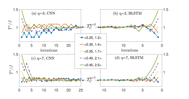
Figure 3: Trajectories of estimated critical temperatures with five different preliminary phase boundaries versus the counts of the iterations from $Step_{1}$ to $Step_{3}$ for 3-state and 7-state Potts models on $24\times 24$ lattices with CNN and BLSTM employed. 1200 preliminary samples labelled in the the first step II.1 are evenly distributed between the temperature $T$ and $T_{low(high)\leavevmode\nobreak\ boundary}$ when $(T_{low\leavevmode\nobreak\ boundary}-T)/J=0.2$ and $(T-T_{high\leavevmode\nobreak\ boundary})/J=0.2$, respectively. In the second step II.2, $S_{1t}$=0.98 and $N_{1}t$=60 in $Step_{1}$. CNN: $\mathcal{C}_{m}$ and $\mathcal{C}_{mm}$ are both that the labels are appointed to the output with larger accuracy. 32 convolutional kernels of size $4\times 4$ are used in the first convolutional layer with strides=1 in both sliding directions. The initial weights and bias are set with a small amount of random values. ‘SAME’ padding is used in both the convolutional operations and max pooling. 64 convolutional kernels are adopted in the second convolutional layer. 1024 neurons are used in both fully connected layers with initial weights and bias same to those of convolutional layers above. 0.5 probability of zeroing is set in the dropout operation. The output of the second fully connected layer runs through the softmax operation, to construct the cross-entropy cost function which would be minimized by Adma algorithm learning rate varies as $0.0001\times 0.99^{k}$ where $k$ denotes the number of training batches cost. Max pooling takes $2\times 2$ window, and strides 2; BLSTM: the criteria $\mathcal{C}_{m}$ and $\mathcal{C}_{mm}$ are that the labels are appointed to the output with accuracy of 0.2 larger. Adma algorithm is also used to minimize the cross-entropy cost function constructed by the output and labels with fixed learning rate 0.001 and 256 LSTM neurons are used. The legends list the preliminary phase boundaries in the format: $<T_{low\leavevmode\nobreak\ boundary},T_{high\leavevmode\nobreak\ boundary}>$ in units of $J$. TensorFlow has been used to implement the neural networks tensorflow2015 . The codes are given in the supplementary material SpMl .

III.3.2 The bidirectional recurrent neural network with long short-term memory units

Recurrent neural networks have the framework of feeding the output of hidden layers back into themselves. This makes them expert in dealing with sequential data where the order of context is significant NN6185 .

Like CNNs, RNNs can also be trained using Adam algorithms in back-propagation process. Merely, in trivial RNNs, gradient usually vanishes for long distance between input and target which limits their applications from learning long-term dependencies arxiv12115063 . LSTM was designed to remedy this problem with memory blocks regulating the flow of information instead of simple sigmoid cells: $Sigmoid(x)=\frac{e^{x}}{(e^{x}+1)}$, in the hidden layers JMLR3115 ; NC91735 . The blocks consist of cells with a forget gate, an input gate and an output gate to control the influence of past on current flow, input and output by multiplying the corresponding weights with biases usually added. Sigmoid functions are usually used to regulate the results in these gates JMLR3115 .

Unlike trivial RNNs, bidirectional recurrent neural networks were invented to utilize the information both from the past and future of a sequence by merging two RNNs with information propagating in opposite directions into one output IEEE4511 ; IEEE799 . This structure makes the networks learn more correlative information of training sequences and be most sensitive to the values around currently evaluate time point. During training, forward and backward states do not interact with each other. After forward and backward processes are done, the network would be updated by minimizing cost functions through back-propagation. Applying LSTM units in trivial bidirectional recurrent neural networks, one gains the BLSTM as shown in Fig.1 which we will use in this work.

To classify the configurations by a BLSTM, different to CNN, the order of rows of configurations acts as time step and each row is treated as the input at the corresponding time step. For the configurations with size $L_{x}\times L_{y}$, we handle $L_{y}$ sequences of length $L_{x}$ for each configuration. One training iteration of the BLSTM follows: Samples at $T/J$ $\rightarrow$ Forward and backward cells of LSTM merge into one output $\rightarrow$ Calculate loss by processing cross-entropy cost function with Softmax operation $\rightarrow$ Employ Adam algorithm to minimize the cost function.

The function of BLSTM in this proposal is same to the CNN above. Besides these two architectures, other powerful neural networks, such as variations of LSTM neural networks, ResNet and deeper neural networks are also highly recommended to act as such a module in this proposal to extract characteristics for general statistical models HBTNN3361 ; Goodfellowbook ; arXiv151203385 .

III.4 The estimating results

As shown by the results of SVD in Fig. 2 (a) and (b), the configurations for 3-state and 7-state Potts models can be divided into two phases versus temperature which are confirmed by the results of Metric-MDS in the insets. It can be seen that the critical points locate near $T/J=1$ for 3-state Potts model and $T/J=0.8$ for 7-state Potts model which approximate theoretical value $T_{c}=1/\log(1+\sqrt{q})$. This pretreatment also offers the thresholds for the preliminary phase boundaries. At high temperature phases, the disordered configurations with spin values which distribute obeying detailed balance, lead to the plateaus of $P_{1}$. This corresponds to the isotropic distributions of the projected points in the Metric-MDS. Both at very low temperature region, the neighbor spins tend to take same values and when temperature is very high, the neighbor spins tend to be different. In both the cases, the fluctuations distribute homogeneously across the lattice which results to the low value of $P_{1}$. Thus it is necessary to use Metric-MDS to reveal the phase scenarios more discreetly. At low temperature phase, the projected points tend to form centers along the central axes of the distributions in Metric-MDS.

The obtuse and sharp turning behaviors of $P_{1}$ near the critical points correspond to the physical features of continuous and first order phase transitions of 3-state and 7-state Potts models, respectively. While there is no more than one dominant maximal singular value in the temperature region, the first two leading principal components are enough to reveal the phase scenarios if one desires to use principal components analysis in the first step. Merely the data should be centered by subtracting the mean values.

According to the results above, the thresholds for the preliminary boundaries for low and high temperature phases can be set as $T_{boundary}$=0.25 and 1.2 in units of $J$, respectively. Then the samples with temperatures outside the region ($0<T/J<0.25$ and $T/J>1.2$) can be assigned low and high temperature labels, respectively. Even there is fluctuation to choose these boundaries, supervised learning tools would be employed to compensate this indeterminacy. Thus different initial phase boundaries would be checked to show the validity of this proposal. Starting from the above results, the critical temperatures for 3-state and 7-state Potts models can be estimated according to the iterations from $Step_{1}$ to $Step_{3}$ in II.2. In Fig.3, along with the iterations, the estimations for the critical temperatures converge to the theoretical values in all the cases. With the same parameters, the critical temperature of 7-state Potts model is more easier to be estimated than that of 3-state Potts model both for the neural networks being CNN and BLSTM. This performance may be related to the characteristics of continuous and first order phase transitions. For the samples on two sides in the vicinity of the critical points, the characteristics are more legible to be learned for first order phase transitions than continuous phase transitions. This corresponds to the behaviors of $P_{1}$ near the critical temperatures in Fig.2. However we do not exclude the influence of $q$ values to the learning results of the neural networks. Although both the CNN and the BLSTM perform well at estimating the critical temperatures for both the models, the estimation by BLSTM converges more quickly than that by CNN. Merely there is little comparability between these results since their mechanisms of recognition are different. This hints that other supervised machine-learning tools with different learning mechanisms may also perform well. And the results indicate that it may be worthy to investigate the relation between the performance of machine-learning tools in learning statistical models and the universal scaling behaviors for those models.

IV Summary

In this work, we show the proposal combining techniques used in dimensionality-reduction processes and neural networks used in supervised learning to estimate critical points for statistical models. And the proposal is demonstrated by two q-state Potts models with different kinds of phase transitions. Actually, this proposal is an iterative approach to assign labels from margins towards center with high accuracy only starting from configurations with corresponding temperatures. The unsupervised pretreatment in the first step aims to offer preliminary phase boundaries and training samples with supervised labels which would be used subsequently by neural networks to estimate critical temperatures more accurately. The determination of phase scenarios and preliminary phase boundaries in the first step is not only necessary for the subsequently step but also indispensable for its application on similar problems. The training set would be enriched during the iteration process, which makes the neural networks be acquainted with the samples more and more accurately. In concrete examples, both a convolutional neural network and a bidirectional recurrent neural network with long short-term memory units perform well at estimating the critical points for two q-state Potts models. With the same neural network, the performances of the estimations for the models correspond to the features of the phase transitions which hints that machine-learning tools may be used to reflect universal scaling laws for statistical models by scientific approaches in the future. Since other machine-learning architectures can also be employed as modules in this proposal, we anticipate that this proposal may work to study new statistical models.

APPENDIX

Updating the parameters like weights of the neural networks play an important role in the learning process. The trained neural networks act like a kind of map architecture. We illustrate the mapping of the networks by a couple of inputs at different phases, weights of trained neural networks and the corresponding outputs. The inputs (matrix here), after multiplied by the matrices of weights in particular manner (like convolutional operation, bias added) up to some regulative activation operations (activation functions, pooling and so on as in section III.3), would be mapped to the corresponding categories (phases). The weights and biases can be updated by algorithms like Adaptive Momentum (adopted in this work), Adaptive Gradient, Momentum and so on. The operations like convolutional operation and structures like gates in LSTM units, make the neural networks extracting characteristics effectively.

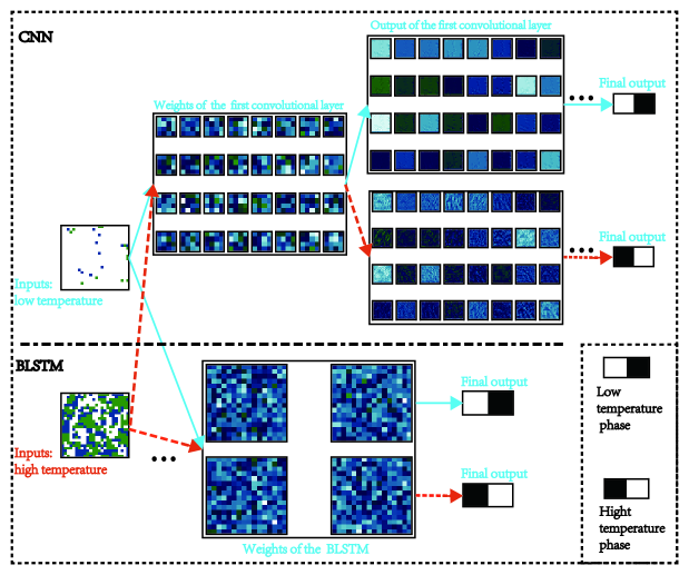
Figure 4: The part above the dot-dashed line: a batch of 32 filters (constructed by weights) in the first convolutional layer and the outputs for two samples at temperatures ($T/J=0.8$) and ($T/J=1.5$) for q=3 Potts model after the CNN has been trained. The part below the dashed line are the weights (reshaped) in the BLSTM. The networks are same to those in Fig. 3. The codes are provided in the supplementary material SpMl .

References

- (1) M. Jordan and T. Mitchell, Machine learning: Trends, perspectives, and prospects, Science 349, 255 (2015).
- (2) Y. LeCun, Y. Bengio, and G. Hinton, Deep learning, Nature (London) 521, 436 (2015).
- (3) M. A. Nielsen, Neural Networks and Deep Learning (Determination Press, 2015)
- (4) I. Goodfellow, Y. Bengio, and A. Courville, Deep Learning (MIT Press, 2016).
- (5) J. Carrasquilla and R. Melko, Machine learning phases of matter, Nat. Phys. 13, 431 (2017).
- (6) L. Wang, Discovering Phase Transitions with Unsupervised Learning, Phys. Rev. B 94, 195105, (2016).
- (7) J. Sebastian, Unsupervised learning of phase transitions: from principal component analysis to variational autoencoders, Phys. Rev. E 96, 022140 (2017).
- (8) W. Hu, R. Singh and R. Scalettar, Discovering Phases, Phase Transitions and Crossovers through Unsupervised Machine Learning: A critical examination, Phys. Rev. E 95, 062122 (2017).
- (9) E. P. L. van Nieuwenburg, Y. H. Liu, and S. D. Huber, Learning phase transitions by confusion, Nat. Phys. 13, 435 (2017).
- (10) K. Ch’ng, J. Carrasquilla, R. G. Melko, and E. Khatami, Machine learning phases of strongly correlated fermions, Physical Review X 7, 031038 (2017).
- (11) Y. Zhang and E.-A. Kim, Quantum Loop Topography for Machine Learning, Phys. Rev. Lett. 118, 216401 (2017).
- (12) Y. Zhang, R. G. Melko, and E.-A. Kim, Machine learning quantum spin liquids with quasiparticle statistics, Phys. Rev. B 96, 245119 (2017).
- (13) P. Zhang, H. Shen, H. Zhai, Machine Learning Topological Invariants with Neural Networks, Phys. Rev. Lett. 120, 066401 (2018).
- (14) N. C. Costa, W. Hu, Z. J. Bai, R. T. Scalettar, and R. R. P. Singh, Principal component analysis for fermionic critical points, Phys. Rev. B 96, 195138 (2017).
- (15) C. Wang and H. Zhai, Machine learning of frustrated classical spin models. I. Principal component analysis, Phys. Rev. B 96, 144432 (2017).
- (16) K. Pearson, On lines and planes of closest fit to systems of points in space, Philos. Mag. 2, 559 (1901).
- (17) I. Jolliffe, Principal Component Analysis (Wiley, 2002).
- (18) C. M. Bishop, Neural Networks for Pattern Recognition (Clarendon, 1996).
- (19) L. Li, T. E. Baker, S. R. White, and K. Burke, Pure density functional for strong correlation and the thermodynamic limit from machine learning, Phys. Rev. B 94, 245129 (2016).
- (20) P. Broecker, J. Carrasquilla, R. G. Melko, and S. Trebst, Machine learning quantum phases of matter beyond the fermion sign problem, Sci. Rep. 7, 8823 (2017).
- (21) P. Mehta and D. J. Schwab, , ,and, An exact mapping between the variational renormalization group and deep learning, arXiv:1410.3831 (2014).
- (22) E. M. Stoudenmire and D. J. Schwab, Supervised Learning with Quantum-Inspired Tensor Networks, Adv. Neural Inf. Process. Syst. 29, 4799 (2016).
- (23) F. Schindler, N. Regnault, and T. Neupert, Probing many-body localization with neural networks, Phys. Rev. B 95, 245134 (2017).
- (24) P. Suchsland and S. Wessel, Parameter diagnostics of phases and phase transition learning by neural networks, Phys. Rev. B 97, 174435 (2018).
- (25) C. Casert, T. Vieijra, J. Nys, J. Ryckebusch, Interpretable Machine Learning for Inferring the Phase Boundaries in a Non-equilibrium System, arXiv:1807.02468 (2018).
- (26) Potts, R. B., Proc. Camb. Some generalized order-disorder transformations, Proc. Camb. Phil. Soc. 48, 106 (1952).
- (27) F. Y. Wu, The Potts model, Rev. Mod. Phys. 54, 235 (1982).
- (28) L. McInnes, J. Healy, J. Melville, UMAP: Uniform Manifold Approximation and Projection for Dimension Reduction, arXiv:1802.03426 (2018).
- (29) J. B. Tenenbaum, and V. de Silva, and J. C. Langford, A Global Geometric Framework for Nonlinear Dimensionality Reduction, Science 290, 2319 (2000).
- (30) S. T. Roweis, and L. K. Saul, Nonlinear dimensionality reduction by locally linear embedding, Science 290, 2323 (2000).
- (31) E. Ising, Beitrag zur Theorie des Ferromagnetismus, Zeitschrift fur Physik 31, 253 (1925).
- (32) L. Onsager, Crystal Statistics. I. A Two-Dimensional Model with an Order-Disorder Transition, Phys. Rev. 65, 117 (1944).
- (33) Baxter, R. J., Potts model at the critical temperature, J. Phys. C. 6, L445 (1973).
- (34) Baxter, R. J., H. N. V. Temperley, and S. E. Ashley, Triangular Potts model at its transition temperature, and related models, Proc. Roy. Soc. London, Ser. A 358, 535 (1978).
- (35) N. Metropolis, S. Ulam, The Monte Carlo Method, J. Am. Stat. Assoc. 44, 335 (1949).
- (36) K. Binder, Applications of Monte Carlo methods to statistical physics, Rep. Prog. Phys. 60, 487 (1997).
- (37) K. Binder and D. W. Heermann, Monte Carlo Simulation in Statistical Physics (Springer-Verlag, 1988)
- (38) Kruskal, J. and Wish, M., Multidimensional Scaling (SAGE, 1978).
- (39) T. Cox, M. Cox, Multidimensional Scaling (Chapman and Hall, London, 1994).
- (40) I. Borg., P. J F Groenen, Modern Multidimensional Scaling: Theory and Applications, Journal of Educational Measurement 40, 277 (2006).
- (41) J. de Leeuw, Applications of convex analysis to multidimensional scaling. J.R. Barra, F. Brodeau, G. Romier, B. van Cutsem (Eds.), Recent Developments in Statistics, North-Holland, Amsterdam, pp 133-145 (1977).
- (42) Supplementary material in the Research Data.
- (43) F. Pedregosa et al., Scikit-learn: Machine Learning in Python, JMLR 12, pp. 2825-2830 (2011).
- (44) H. Gish, A probabilistic approach to the understanding and training of neural network classifiers, in Proc. IEEE Int. Conf. Acoust., Speech, Signal Process, pp:1361-1364 (1990).
- (45) A. Krizhevsky, I. Sutskever, G. E. Hinton, Imagenet classification with deep convolutional neural networks, Advances in neural information processing systems, pp 1097-1105 (2012).
- (46) D. A. Clevert, T. Unterthiner, S. Hochreiter, Fast and accurate deep network learning by exponential linear units (elus), arXiv:1511.07289 (2015).
- (47) V. Nair, G. E. Hinton, Rectified linear units improve restricted boltzmann machines, Proceedings of the 27th international conference on machine learning (ICML-10), pp 807-814 (2010).
- (48) P. Ramachandran, B. Zoph, Q. V. Le, , ,and, Swish: a Self-Gated Activation Function, arXiv:1710.05941 (2017).
- (49) G. E. Hinton, N. Srivastava, A. Krizhevsky, I. Sutskever, R.R. Salakhutdinov, Improving neural networks by preventing co-adaptation of feature detectors, arXiv:1207.0580 (2012).
- (50) N. Srivastava, G. E. Hinton, A. Krizhevsky, I. Sutskever, R. Salakhutdinov, Dropout: A simple way to prevent neural networks from overfitting, The Journal of Machine Learning Research 15, 1929 (2014).
- (51) D. P. Kingma, J. Ba, Adam: A method for stochastic optimization, arXiv:1412.6980 (2014).
- (52) J. Schmidhuber. Deep Learning in Neural Networks: An Overview, Neural Networks, 61, 85 (2015).
- (53) R. Pascanu, T. Mikolov, Y. Bengio, On the difficulty of training Recurrent Neural Networks, arxiv:1211.5063 (2013).
- (54) F. Gers, N. Schraudolph, and J. Schmidhuber. Learning precise timing with LSTM recurrent networks. Journal of Machine Learning Research 3, 115 (2002).
- (55) S. Hochreiter and J. Schmidhuber. Long Short-Term Memory, Neural Computation 9, 1735 (1997).
- (56) M. Schuster and K. K. Paliwal. Bidirectional recurrent neural networks. IEEE Transactions on Signal Processing, 45, 2673 (1997).
- (57) A. Graves, F. Santiago, and S. Jurgen, Bidirectional LSTM networks for improved phoneme classification and recognition. Artificial Neural Networks: Formal Models and Their Applications–ICANN 2005, Springer Berlin Heidelberg, pp 799-804 (2005).
- (58) K. He, X. Zhang, S. Ren, J. Sun, Deep Residual Learning for Image Recognition, arXiv:1512.03385 (2015).
- (59) M. Abadi, et al. TensorFlow: Large-Scale Machine Learning on Heterogeneous Systems, http://tensorflow.org (2015).