Optical Design of PICO, a Concept for a Space Mission to Probe Inflation and Cosmic Origins

Abstract

The Probe of Inflation and Cosmic Origins (PICO) is a probe-class mission concept currently under study by NASA. PICO will probe the physics of the Big Bang and the energy scale of inflation, constrain the sum of neutrino masses, measure the growth of structures in the universe, and constrain its reionization history by making full sky maps of the cosmic microwave background with sensitivity 80 times higher than the Planck space mission. With bands at 21-799 GHz and arcmin resolution at the highest frequencies, PICO will make polarization maps of Galactic synchrotron and dust emission to observe the role of magnetic fields in Milky Way’s evolution and star formation. We discuss PICO’s optical system, focal plane, and give current best case noise estimates. The optical design is a two-reflector optimized open-Dragone design with a cold aperture stop. It gives a diffraction limited field of view (DLFOV) with throughput of 910 cm²sr at 21 GHz. The large 82 square degree DLFOV hosts 12,996 transition edge sensor bolometers distributed in 21 frequency bands and maintained at 0.1 K. We use focal plane technologies that are currently implemented on operating CMB instruments including three-color multi-chroic pixels and multiplexed readouts. To our knowledge, this is the first use of an open-Dragone design for mm-wave astrophysical observations, and the only monolithic CMB instrument to have such a broad frequency coverage. With current best case estimate polarization depth of 0.65 $\mu$K_CMB-arcmin over the entire sky, PICO is the most sensitive CMB instrument designed to date.

1 INTRODUCTION

Over the last decade NASA’s astrophysics division has funded design and construction of space missions that are either Explorer-class, with cost cap of up to $250M or Flagship-class that cost above $1B. To study the science opportunities available at intermediate costs, NASA initiated studies of Probe-class missions with cost window between $400M and $1B. We are conducting one these studies for a mission called the Probe of Inflation and Cosmic Origins (PICO). A paper by Sutin et al.[1] in these proceedings gives an overall review of PICO and the scientific motivation. This paper describes the design of the telescope and focal plane and gives our current best estimates for the sensitivity of the instrument. The mission study is not complete; the final report is due in December 2018. Therefore, the quantitative assessments we provide for component temperatures and detector noise levels are temporary in nature and subject to revision. Even so, the design is fairly mature and we do not expect significant changes. Values in this paper are current best estimates and don’t represent finalized mission requirements.

2 MISSION AND SPACECRAFT

PICO will conduct scientific observations for five years from an orbit around the Earth-Sun L2 Lagrange point. The design had 21 bands centered at 21–799 GHz. The spacecraft design impacted the optical design and sensitivity in two primary ways; volume constraints limited the physical size of the telescope and optical component temperatures impacted noise levels.

The maximum diameter of the spacecraft is limited by the 4.6 m largest diameter that a SpaceX’s Falcon 9 launch vehicle can carry. This diameter limits the V-groove shields’ size, which, along with the scan strategy, defines the ‘shadow cone’ in Figure 1. The shadow cone is the volume protected from solar illumination, and all optical components are contained within it. The shadow cone and inner V-grooves defines an available volume for the telescope. We opted not to use deployable shields as they present added cost and risk which outweighs the benefits. The thermal model indicates the temperatures of the optical elements as given in Figure 1. The primary reflector is passively cooled, while the optics box, secondary reflector, and focal plane are actively cooled; Sutin et al.[1] gives more details of the thermal system.

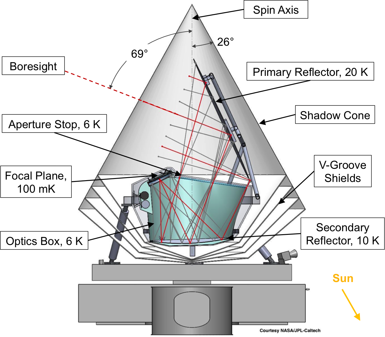
Figure 1: The spin axis of the satellite precesses around the satellite-sun axis (orange arrow) with an angle of 26 deg. This precession defines the shadow cone shown in light gray.

3 OPTICAL SYSTEM

The choice of telescope design is driven by a combination of science requirements and the physical limits discussed in Section 2. The science requirements are: a large diffraction limited field of view (DLFOV) sufficient to support $\mathcal{O}(10^{4})$ detectors, arcminute resolution at 800 GHz, low instrumental polarization, and low sidelobe response. Additionally, the transition edge sensor bolometers baselined for PICO require a telecentric focal plane which is sufficiently flat that it can be tiled by 10 cm detector wafers without reduction in optical quality.

To increase aperture efficiency and reduce sidelobes we concentrated our investigation around off-axis optical designs. More than 30 years ago Dragone analyzed the performance of several off-axis systems and found solutions with low cross-polarization at the center of the field of view and with astigmatism, or astigmatism and coma, canceled to first order.[2, 3, 4] These systems also have no cross-polarization at the center of the field of view. A number of recent CMB instruments used off-axis systems, and several began the design optimization with systems based on designs by Dragone[5, 6, 7, 8, 9, 10]. For PICO we began the optimization with a two-reflector Dragone system that, to our knowledge, has not been implemented in CMB instruments before. We call it an ‘open-Dragone’ because of its overall geometry and in contrast to the widely used ‘cross-Dragone’, see Figure 3. We used a 1.4 m entrance aperture as this aperture diameter satisfies the science requirements.

We considered two additional Dragone systems, a Gregorian Dragone and a cross-Dragone, and compared the relative performance of all three systems in terms of DLFOV, compactness, and rejection of sidelobes. Compared to the open-Dragone, the Gregorian had half the DLFOV for the same $F$-number and could not support $\mathcal{O}(10^{4})$ detectors. It was therefore rejected. The cross-Dragone had roughly $4\times$ the DLFOV of the open-Dragone, but was more difficult to pack inside the spacecraft volume while avoiding the known sidelobes shown in Figure 2. We found that the largest cross-Dragone which met the PICO volume constraints had a 1.2 m aperture and an $F$-number of 2.5, while the largest open-Dragone aperture was 1.4 m with an $F$-number of 1.42. The larger $F$-number of the cross-Dragone system implied a larger physical focal plane, and therefore higher mass and cost, for the same number of pixels. For the PICO case, we concluded that the advantages of a low $F$-number and easily baffled sidelobes made the open-Dragone a good starting point for further optimization.

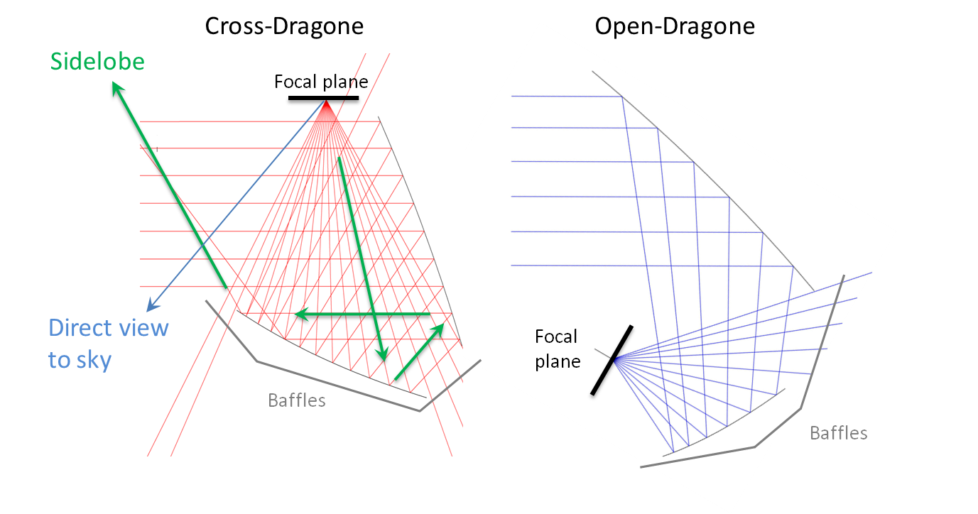
Figure 2: Comparison of sidelobes for a cross-Dragone (left) and an open-Dragone (right). Rays were traced from the center of the focal plane toward the sky. For both systems spillover around the secondary was straightforward to mitigate with absorptive baffles. However, the rays labeled ‘sidelobe’ and ‘direct view to sky’ in the cross-Dragone system presented added challenges. Those challenges could be mitigated—with a long forebaffle or larger $F$-number (see for example Matsumrua et al.[9])—but doing so increased the overall physical size of the system, which was problematic in the PICO case.

We designed the initial open Dragone following Granet’s method[11]. We began with a solution with $F=1.42$, a 1.4 m aperture (that was verified to satisfy the volume constraints), and a large DLFOV. We forced a circular aperture stop between the primary and secondary reflectors and numerically optimized its angle and position to obtain a larger DLFOV. The stop diameter was chosen such that for the center feed it projected a 1.4 m effective aperture onto the primary. Adding a stop in this way increased the size of the primary reflector, because different field angles illuminated different areas on the reflector. Actively cooling the aperture stop, however, reduced detector noise, and the stop shielded the focal plane from stray radiation. At this stage the system still met the Dragone condition and is defined by the ‘Initial Open-Dragone’ parameters in Table 1.

In his publications Dragone provides a prescription to eliminate coma in addition to the cancellation of astigmatism that is inherent to the baseline designs.[3] The corrections involve adding distortions to the primary and secondary reflectors which are proportional to $r^{4}$ where $r=0$ is at the chief ray impact point on each reflector. We thus attempted to increase the DLFOV using two methods.

In ‘Method1’, one of the coauthors (RH) used Zemax to add Zernike polynomials to the base conics which described the reflectors. These Zernike polynomials were offset from the symmetry axis of the conic by $624.2$ cm for the primary and $76.1$ cm for the secondary. This placed the origin of polynomials at the chief ray impact point for each reflector. Inspired by the Dragone corrections, all Zernike terms up to fourth order and the first fifth order term were allowed to vary. The optimization metric was minimization of the rms spot diameter at the following locations: the center of the FOV, $\pm 2$ deg in Y, and $\pm 4$ deg in X. The center of the FOV was given a weight of 100 while each outer point was given a weight of 1. To constrain the optimization, the X and Y effective focal lengths were held fixed as was the impact point of the chief ray on the focal plane. This optimization step increased the DLFOV by factors of 1.15, 2.4 and 10.5 at 21, 155 and 799 GHz, respectively. We further increased the DLFOV by approximately 50% at all frequencies by including a curved focal surface and rerunning the optimization. A small ($\sim$4%) additional gain in DLFOV was achieved by adding Zernike terms up to sixth order, allowing the secondary to focal surface distance to vary, adding a weighted constraint on the effective focal length, and adding fields with weight of 0.01 to the rms spot diameter metric at $\pm 7.5$ deg in Y and $+15$ deg in X. These additional fields were necessary to constrain the corrections at the reflector edges.

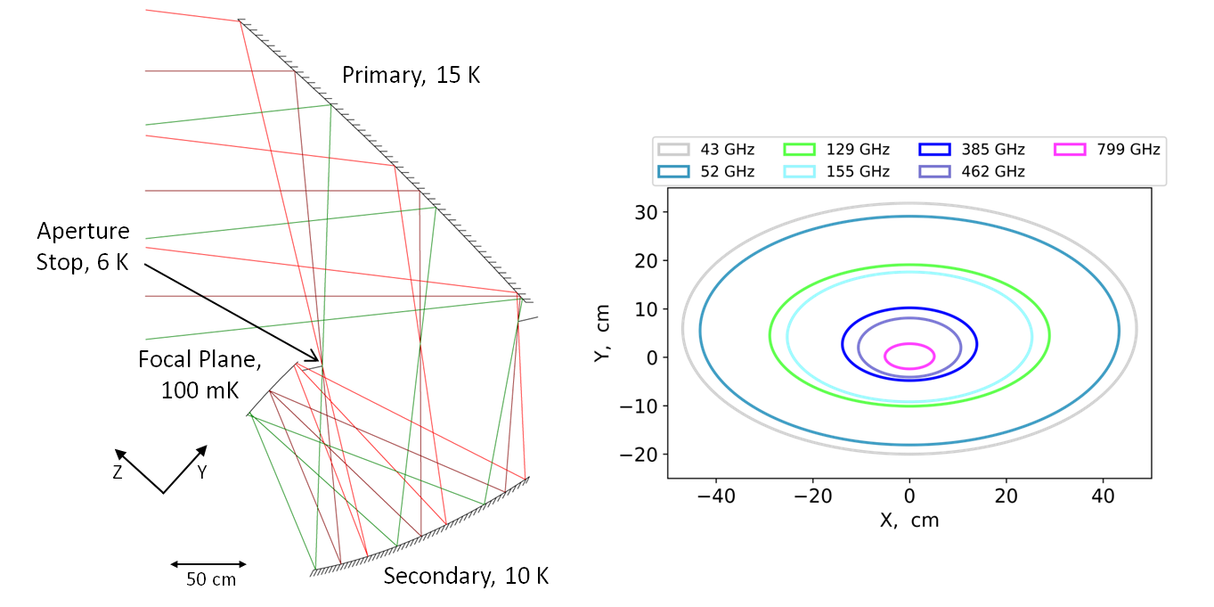
Figure 3: Raytrace (left) and Strehl $=0.8$ contours (right) for the PICO optical design.

Table 1: Telescope geometric parameters

PICO optical system					Initial Open-Dragoneb
	Primary	Secondary	Telescope parametersb		Design parameters
Reflector sizea (cm)	$270\times 205$	$160\times 158$	Aperture (cm)	140	Aperture (cm)	140
Radius of curvature (cm)	$\infty$	136.6	$F$-number	1.42	$\theta_{0}$ (deg)	90
Conic constant, $k$	0	-0.926	h (cm)	624.2	$\theta_{e}$ (deg)	20
4th ZCc (cm)	2018.4	-61.1	$\alpha$ (deg)	74.2	$\theta_{p}$ (deg)	140
9th ZC (cm)	-37.0	16.7	$\beta$ (deg)	62.3	Lm (cm)	240
10th ZC (cm)	-2919.8	-15.1	Lm (cm)	229.3
11th ZC (cm)	-1292.7	22.3	Ls (cm)	140.5	Derived parameters
12th ZC (cm)	120.6	-3.8			$F$-number	1.42
13th ZC (cm)	-74.5	4.9	Focal Surface		h (cm)	624.2
19th ZC (cm)	-75.8	3.4	Ellipse major axes (cm)	69 x 45	$\alpha$ (deg)	38.6
20th ZC (cm)	-398.9	6.3	Ellipse major axes (deg)	19 x 13	$\beta$ (deg)	101.4
21st ZC (cm)	-319.5	23.3	Radius of curvature (cm)	455	Ls (cm)	122.2
22nd ZC (cm)	-276.6	-8.5			Primary, $f$ (cm)	312.1
23rd ZC (cm)	-201.6	-3.2			Secondary, $a$ (cm)	131
24th ZC (cm)	-127.4	-1.9			Secondary, $e$	1.802
25th ZC (cm)	-55.0	0.1
a The maximum physical size of the reflectors.
b Telescope parameters follow the definitions in Granet 2001.[11]
c ZC = Zernike Coefficient; the ZC normalization radius for the Primary (Secondary) mirror is 524.8 (194.1) cm

In ‘Method2’ another coauthor (JM) used CodeV and allowed additional geometric parameters of the system to vary. To adjust the reflector shapes, we added Zernike polynomial corrections to the conic surfaces which defined the two reflectors. The Zernike polynomials were defined in the same coordinate systems as the base conics. We varied the 4th and 9th-13th Zernike coefficients. We allowed the focal surface curvature and focal surface to secondary distance L_s to vary. The primary-secondary distance L_m, primary offset $h$, and the primary and secondary rotation angles, $\alpha$ and $\beta$, were varied as well. The optimization metric was the rms spot diameter across the field of view, with weighted constraints requiring telecentricity and maintaining the X- and Y-focal lengths. We added Lagrange constraints to enforce beam clearances and place an upper limit on overall system size. Once the optimization converged to an acceptable optical system, we added higher order Zernike terms, 19th-25th, and refined the reflector shapes using the same metric and constraints. The current PICO optical design is from the Method2 optimization procedure.

Figure 4 shows that Method2 greatly increased the DLFOV relative to the initial open-Dragone design. The DLFOV increased by factors of 1.9, 3.8, 4.3, and 4.6 at 21, 129, 155, and 799 GHz, respectively. The most important gain was at frequencies of 129 and 155 GHz. We used this extra area to add more C and D pixels, see Figure 5 and Section 4. The C and D pixels contained the bands most sensitive to the CMB, and adding hundreds of these pixels into the focal plane gives PICO unprecedented levels of CMB sensitivity. Method2 gave somewhat better performance at lower frequencies with a DLFOV 1.11 and 1.15 times larger than Method1 at 21 and 155 GHz, respectively. At 799 GHz Method2 gave DLFOV only 0.3 times that of Method1’s area, but the DLFOV still satisfied our science requirements. Figure 4 also shows that Method2 reduced the overall telescope volume and gave more physical margin relative to the shadow cone.

The geometric parameters of the PICO optical system are given in Table 1. The system is diffraction limited for 799 GHz at the center of the field of view. At 155 GHz the DLFOV is 82.4 deg² and the total throughput at 20 GHz is 910 cm²sr. Figure 3 shows Strehl of 0.8 contours for all pixel types. The slightly concave focal surface, which has a radius of curvature of 4.55 m, is telecentric to within 0.12 deg across the entire FOV.

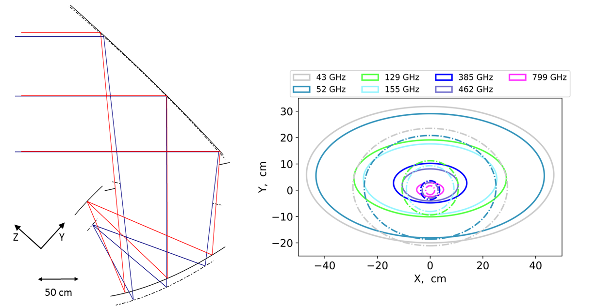
Figure 4: Comparison between the Method2 open-Dragone and the initial open-Dragone. The ray traces (left) are aligned at the chief ray impact point on the primary. The final optical system, optimized with Method2 (red rays, solid reflectors), was smaller in the vertical direction than the initial open-Dragone (blue rays, dash-dot reflectors). The overlaid Strehl $=0.8$ contours (right) show the improvement achieved with Method2 at all frequencies (solid lines) vs the initial open-Dragone (dash-dot lines) system.

An additional benefit of the optimization is the radius of curvature of the concave focal surface. The open-Dragone’s focal surface is naturally curved. Matching this curvature reduces defocus, increases the DLFOV, and increases telecentricity. The unoptimized system was telecentric to within 2.5 deg while the optimized version is telecentric to within 0.12 deg. If the focal surface was too strongly curved tiling it with flat detector wafers would result in large defocus at the edges of these wafers. This is not the case for PICO. The 4.55 m focal surface radius of curvature, results in a defocus of 0.1 mm at the edge of a 10 cm wafer.

4 FOCAL PLANE

Modern mm/sub-mm bolometers are photon noise limited. An effective way to increase sensitivity is to increase the number of detectors in the focal surface. The PICO focal surface has 12,996 detectors, 175 times the number flown on Planck. PICO achieves this by having a large DLFOV and using multichroic pixels (MCPs)[12, 13]. The MCP architecture assumed for PICO has three bands per pixel with two single polarization transition edge sensor (TES) bolometers per band and therefore six bolometers per pixel. We assume the MCPs were coupled to free space using lenslets and sinuous antennae [12], but the pixel sizes, numbers, and spacing would not change significantly if horn or phased array coupling would be used instead.

PICO has 21 overlapping bands with centers spanning the range 21–799 GHz. The bands are divided amongst nine pixel types labeled A to I; see Figure 5. The 25% fractional bandwidth is broader than the interband spacing causing neighboring bands to overlap and requiring them to be in separate pixels. The exceptions to the MCP architecture are the highest three bands, because they are above the superconducting band gap of the niobium used for transmission lines, antennae, and filters in MCPs. For bands G, H, and I, we assume feedhorn-coupled polarization sensitive bolometers. The technology has high TRL as it has been used successfully with Planck[14] and Herschel SPIRE[15].

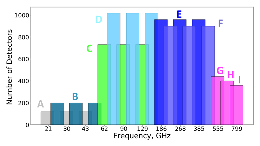
Figure 5: Frequency coverage of the PICO bands. Each color (excluding magenta) denotes a different MCP, labeled A-F. The bar height indicates the number of detectors per band. Bar width gives the bandwidth. All bands are top-hats with 25% fractional bandwidth; the $x$-axis is logarithmic. The three highest frequencies (magenta) are the single color pixels G, H, and I.

Figure 6 shows the PICO focal plane. We optimized the diameter of each MCP by calculating the array sensitivity for that pixel type. The calculation included the increasing illumination of the aperture stop as the pixel diameter decreased, as described in Section 5.1. We chose a pixel diameter of $2.1$F$\lambda_{\rm mid}$, where $\lambda_{\rm mid}$ refered to the center band of each pixel. This gave an edge taper, $T_{e}$, on the stop of 10 dB for the center band of each pixel.

Figure 6: Left: PICO focal plane layout with Strehl $=0.8$ contours for each pixel type. The pixel and Strehl contour colors match the band colors, A-I, in Figure 5. Right: Layout of pixels sensitive to Stokes Q (black crosses) and Stokes U (red exes) for an example wafer.

Differencing detectors sensitive to orthogonal polarization states enables each pixel to make a measurement of a particular Stokes parameter. Pixels sensitive to the $U$ Stokes parameter are rotated by 45 deg relative to those that are sensitive to $Q$. This Q/U alignment is in the instrument reference frame with the $x$-axis parallel to the scan direction; see Figure 6.

The PICO focal plane readout is designed around $\times$128 time domain multiplexing (TDM), but this choice is not a significant driver for the focal plane layout or overall noise budget.

5 INSTRUMENT NOISE

We developed an end to end noise model of the PICO instrument to predict full mission sensitivity and provide a metric by which to evaluate mission design trade-offs. This model assumed white noise at all frequencies. The overall sensitivity did not include calibration uncertainties or estimates of other possible systematic effects. To construct the model we estimated the optical load, calculated noise equivalent power (NEP) by source, combined all NEP terms to get detector noise, combined all detectors to get noise per frequency band, and then included total mission time to find overall mission sensitivity.[16, 17] Each of these steps included various assumptions and design decisions, which are discussed in this section. The assumptions are summarized in Table 2. The values presented in this section are current best case estimates. Instrument noise requirements, which would have larger noise levels, are still being determined.

To validate our calculations we compared two independent codes that were used for several CMB instruments. The calculations agreed within 1% for individual noise terms and for overall mission noise. We also used our model to calculate CORE [8] and LiteBIRD [9, 18] noise from their published system parameters. The results were consistent with published values when similar assumptions were used.

Table 2: Noise model parameters, see text for details.

Throughput	single moded, $\lambda^{2}$
Fractional Bandwidth	25%
Reflector emissivity	$\epsilon=\epsilon_{0}\sqrt{\nu/\text{150~{}GHz}},\epsilon_{0}=0.07\%$
Aperture stop emissivity	1
Low pass filter reflection loss	8%
Low pass filter absorption lossa	frequency dependent, 0.2%–2.8%
Bolometer absorption efficiency	70%
Te of low, middle, and high bands (dB)	4.8, 10.0, 20.7
$\eta_{\rm stop}$ of low, middle, and high bands	0.68, 0.90, 0.99
Bose noise fraction, $\xi$	1
Bolometer yield	90%
Bath temperature, $T_{o}$ (mK)	100
TES critical temperature, $T_{c}$ (mK)	187
Safety factor, Psat/Pabs	2
Thermal power law index, $n$	2
Intrinsic SQUID noise (aW/$\sqrt{\text{Hz}}$)	3
TES operating resistance, $\Omega$	0.03
TES transition slope, $\alpha$	100
TES loop gain	14
Mission length (years)	5
Observing efficiency	95%
aAssumes different thickness per pixel type.

5.1 Single bolometer noise

5.1.1 Model

The sources of optical load are the CMB, the primary and secondary reflectors, the aperture stop, and low pass filters. These elements are shown schematically in Figure 7. The total load absorbed at the bolometer is the sum of the power emitted by each element reduced by the transmission efficiency of the elements between the emitting surface and the bolometer. The absorbed power is

$$P_{\rm abs}=((((P_{\rm CMB}\eta_{\rm PRI}+P_{\rm PRI})\eta_{\rm stop}+P_{\rm stop}(1-\eta_{\rm stop}))\eta_{\rm SEC}+P_{\rm SEC})\eta_{\rm filter}+P_{\rm filter})\eta_{\rm bolo},$$ (1)

where $P_{\rm elem}$ is the in-band power emitted by a given element for a single polarization and $\eta_{\rm elem}$ is the transmission efficiency of the element. Power emitted by the stop is a special case. We multiply $P_{\rm stop}$ by $(1-\eta_{\rm stop})$ because $\eta_{\rm stop}$ is the spillover efficiency, the fraction of the throughput passing through the stop. Therefore $(1-\eta_{\rm stop})$ is the fraction of the throughput which views the stop. We determine $\eta_{\rm stop}$ in the following way. The MCP angular beam width depends on the wavelength and pixel diameter as[16]

$$\theta_{1/e^{2}}=\frac{2.95\lambda}{\pi D_{\rm px}}.$$ (2)

We fix $D_{\rm px}$ such that the edge taper, T_e, of the middle frequency band in each pixel is 10 dB and calculate T_e for the upper and lower bands using Equation 2. This changing illumination of the stop is shown schematically by the dashed rays in Figure 7. For each MCP in pixels A-H, T_e is 4.8, 10, and 20.7 dB for the lower, middle, and upper bands, respectively. These edge tapers correspond to $\eta_{\rm stop}$ of 0.68, 0.90, and 0.99. The changing $\eta_{\rm stop}$ has two main effects: changing illumination efficiency between bands, which affects optical load and therefore the noise equivalent temperature (NET); and telescope beam size not scaling smoothly with $\lambda$. The left panel of Figure 8 gives the optical load as a function of frequency. The jumps in load between neighboring bands near 70 and 200 GHz, are due to $\eta_{\rm stop}$ changing with frequency.

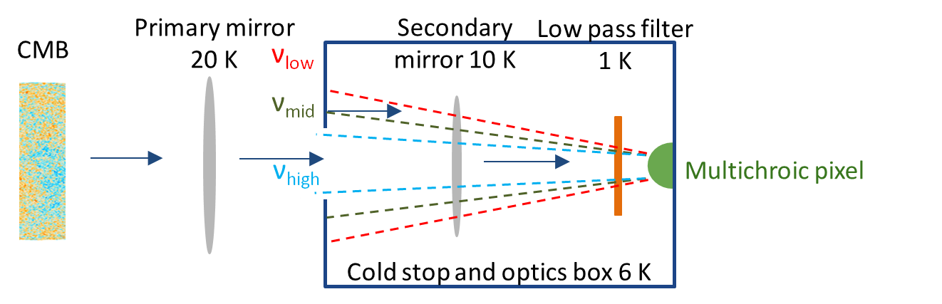
Figure 7: Schematic representation of the prediction of optical load. Power emitted by each element was modified by the efficiency of the following elements and added to the total expected load. The multichroic pixel illuminated the stop differently for each of the three bands.

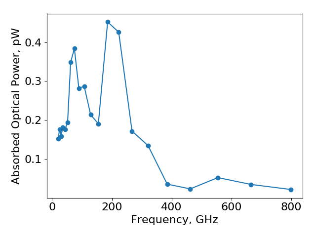
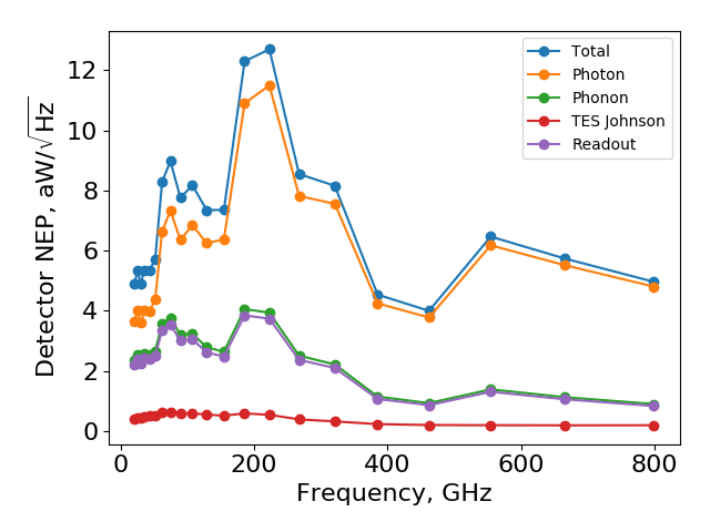
Figure 8: Left: Expected optical load as a function of frequency for single polarization PICO bolometers. Center: Breakdown of NEP sources across the PICO frequency range. Photon noise dominates even at the lowest frequencies. Right: Single detector NET for the PICO bands.

We consider four noise sources per bolometer; photon, phonon, TES Johnson, and readout. Photon noise depends on the absorbed power[19]

$$NEP_{\gamma}^{2}=\int\limits_{\rm band}2h\nu p_{\nu}\,d\nu+2\xi\int\limits_{\rm band}p_{\nu}^{2}\,d\nu,$$ (3)

where $p_{\nu}$ is the power spectral density for a single polarization absorbed at the bolometer and $\xi=1$ is the fraction of correlated Bose photon noise. We included a factor of 2 in the Bose noise term because the bolometers received power from a single polarization. Using $P_{\rm abs}$ we calculate the TES bolometer properties and phonon noise.[20] We calculate TES Johnson noise, which depends on bolometer bias parameters, for each frequency band. All noise sources in the cold and warm readout electronics are lumped under the readout term. The combined NEP and the NEP per noise source are shown in Figure 8 as a function of frequency; the combined values are given in Table 3.

5.1.2 Results

The primary contributor to noise is the optical load; see Figure 8. The CMB and stop account for the majority of the optical load at all frequencies. Even at 800 GHz the 6.5 K stop contributes 53% of the total radiative power compared to 47% coming from the mirrors. The CMB gives more than half the load in the middle and upper bands of the multichroic pixels, but the stop dominates the load in the lowest band of each pixel. Load from the stop in the lowest band of each pixel ranges from 1.2 times the CMB load at 21 GHz to a maximum of 4.7 times the CMB load at 223 GHz.

Bose noise is most significant at lower frequencies with NEP_Bose/NEP${}_{\rm Poisson}=1.5$ in the lowest band. (All NEP ratios are calculated using units of W/$\sqrt{\rm Hz}$ for the dividend and divisor.) However, Poisson noise increases as $\sqrt{P_{\rm abs}\nu}$ while Bose is proportional to $P_{\rm abs}$. Poisson noise equals Bose noise at 30 GHz and dominates at higher bands; NEP_Bose/NEP${}_{\rm Poisson}<10\%$ at 321 GHz. Phonon noise is the second most significant source, NEP_phonon/NEP_photon ranges from 65% at 21 GHz to 19% at 799 GHz.

For TDM readout, phonon and readout noise are approximately equal, and TES Johnson noise is insignificant. We also modeled noise for frequency domain multiplexing readout (FDM). For FDM the TES Johnson noise is higher, 2/3 of the readout NEP, but the readout noise is lower. Comparing the combined TES Johnson and readout NEPs for TDM and FDM we find essentially identical performance with total noise differing by less than 3% across all bands.

As mentioned in the beginning of Section 5, the detector NEP we calculate for PICO is consistent with that calculated for CORE [8] and for LiteBIRD [9, 18] when accounting for different input parameters such as the center frequencies, bandwidth, and aperture illumination efficiency as a function of frequency.

5.2 Combined array noise

Using single detector NEPs from Section 5.1, the detector counts from Section 4, and 90% yield for each frequency band (see Table 2) we calculate the combined NEP of the detector array for each band. Combining $N$ detectors reduces uncorrelated noise by $\sqrt{N}$. This scaling does not hold for Bose photon noise. For the lowest band of each MCP the pixel spacing is $0.4$F$\lambda$ and thus the pixels oversample the point spread function leading to correlated photon noise between pixels. Accounting for this effect gives a 26% increase in the combined array NEP for the 21 GHz band and a 0.003% increase at 799 GHz. From the array NEP we convert to noise equivalent temperature (NET) per band using Numerical values for the NET are given in the second to last column in Table 3.

Assuming evenly weighted observations of the full sky, 5 years of mission duration, and 95% efficiency, we calculate full mission map sensitivities in polarization; see the final column in Table 3. Combining all bands gives a total CMB map depth for the entire PICO mission of 0.65 $\mu$K_CMB-arcmin.

Table 3: PICO frequency channels and noise.

Pixel	Band	FWHM	Bolometer NEP	Bolometer NET	Nbolo	Array NET	Polarization map depth
Type	GHz	arcmin	aW/$\sqrt{Hz}$	$\mu$K${}_{\rm CMB}\sqrt{s}$		$\mu$K${}_{\rm CMB}\sqrt{s}$	$\mu$KCMB-arcmin	Jy/sr
A	21	38.4	4.89	112.2	120	13.6	19.1	6.69
B	25	32.0	5.33	103.0	200	9.56	13.5	7.98
A	30	28.3	4.92	59.4	120	5.90	8.30	7.93
B	36	23.6	5.36	54.4	200	4.18	5.88	9.59
A	43	22.2	5.33	41.7	120	4.01	5.65	13.9
B	52	18.4	5.73	38.4	200	2.86	4.03	16.8
C	62	12.8	8.29	69.2	732	3.14	4.41	37.0
D	75	10.7	8.98	65.4	1020	2.46	3.47	48.1
C	90	9.5	7.76	37.7	732	1.49	2.09	44.5
D	108	7.9	8.18	36.2	1020	1.21	1.70	57.0
C	129	7.4	7.35	27.8	732	1.08	1.53	69.7
D	155	6.2	7.36	27.5	1020	0.91	1.28	84.6
E	186	4.3	12.30	70.8	960	2.51	3.54	383
F	223	3.6	12.70	84.2	900	3.05	4.29	579
E	268	3.2	8.55	54.8	960	1.87	2.63	369
F	321	2.6	8.16	77.6	900	2.73	3.84	518
E	385	2.5	4.54	69.1	960	2.35	3.31	318
F	462	2.1	4.00	132.6	900	4.66	6.56	403
G	555	1.5	6.47	657.8	440	33.1	46.5	1569
H	666	1.3	5.74	2212	400	117	164	1960
I	799	1.1	4.97	10433	360	580	816	2321
Total					12996	0.46	0.65

6 CONCLUSIONS/SUMMARY

The PICO optical system is a two reflector open-Dragone design. It gives a large DLFOV and a total throughput larger than 900 cm²sr without lenses. The use of a system with only reflectors, as opposed to a combination of reflectors and refractors, gives the system high transmission efficiency across a wide frequency band and obviates the need to provide broad band anti-reflection coatings. Using only two reflectors reduces the volume, mass, and complexity of the system compared to designs with more reflectors. The optical system has a cold aperture stop between the primary and secondary reflectors. The stop reduces sidelobes while maintaining the other reflectors compact. The native Dragone system has been numerically optimized using Zernike polynomials to give a significantly larger DLFOV.

The focal plane takes advantage of the large DLFOV and MCP technology using TES bolometers to implement 12996 polarization sensitive detectors in 21 bands from 21-799 GHz. This is the first monolithic CMB instrument to have sensitivity to such a broad frequency range and to baseline a single detector technology across this entire band. Under the current set of assumptions, PICO is predicted to have an unprecedented full sky polarization map depth of 0.65 $\mu$K_CMB-arcmin, which is $\sim$80 times the depth Planck had achieved.

7 ACKNOWLEDGMENTS

This Probe mission concept study is funded by NASA grant #NNX17AK52G. Gianfranco de Zotti acknowledges financial support from the ASI/University of Roma–Tor Vergata agreement n.  2016-24-H.0 for study activities of the Italian cosmology community. Jacques Delabrouille acknowledges financial support from PNCG for participating in the PICO study.

References

- [1] Sutin, B. M., Alvarez, M., Battaglia, N., et al., “PICO - the probe of inflation and cosmic origins,” Proc. SPIE 10698 (2018).
- [2] Dragone, C., “Offset multireflector antennas with perfect pattern symmetry and polarization discrimination,” Bell Labs Technical Journal 57(7), 2663–2684 (1978).
- [3] Dragone, C., “First-order correction of aberrations in Cassegrainian and Gregorian antennas,” IEEE Transactions on Antennas and Propagation 31, 764–775 (September 1983).
- [4] Dragone, C., “Unique reflector arrangement with very wide field of view for multibeam antennas,” Electronics Letters 19(25), 1061–1062 (1983).
- [5] Fargant, G., Dubruel, D., Cornut, M., et al., “Very wide band telescope for Planck using optical and radio frequency techniques,” in [UV, Optical, and IR Space Telescopes and Instruments ], Breckinridge, J. B. and Jakobsen, P., eds., Proc. SPIE 4013, 69–79 (July 2000).
- [6] Swetz, D. S., Ade, P. A. R., Amiri, M., et al., “Overview of the Atacama Cosmology Telescope: Receiver, Instrumentation, and Telescope Systems,” ApJS 194, 41 (June 2011).
- [7] Padin, S., Staniszewski, Z., Keisler, R., et al., “South Pole Telescope optics,” Appl. Opt. 47, 4418–4428 (Aug. 2008).
- [8] de Bernardis, P., Ade, P. A. R., Baselmans, J. J. A., et al., “Exploring cosmic origins with CORE: The instrument,” Journal of Cosmology and Astro-Particle Physics 2018, 015 (Apr. 2018).
- [9] Matsumura, T., Akiba, Y., Arnold, K., et al., “LiteBIRD: Mission Overview and Focal Plane Layout,” Journal of Low Temperature Physics 184, 824–831 (Aug. 2016).
- [10] Parshley, S., Niemack, M., and Hills, R. E., “The optical design of the six-meter CCAT-prime and Simons Observatory telescopes,” Proc. SPIE 10700 (2018).
- [11] Granet, C., “Designing classical Dragonian offset dual-reflector antennas from combinations of prescribed geometric parameters,” IEEE Antennas and Propagation Magazine 43, 100–107 (Dec. 2001).
- [12] Suzuki, A., Arnold, K., Edwards, J., et al., “Multi-chroic dual-polarization bolometric detectors for studies of the cosmic microwave background,” Journal of Low Temperature Physics 176, 650–656 (Sep 2014).
- [13] Datta, R., Hubmayr, J., Munson, C., et al., “Horn Coupled Multichroic Polarimeters for the Atacama Cosmology Telescope Polarization Experiment,” Journal of Low Temperature Physics 176, 670–676 (Sept. 2014).
- [14] Lamarre, J. M., Puget, J. L., Ade, P. A. R., et al., “Planck pre-launch status: The HFI instrument, from specification to actual performance,” A&A 520, A9 (Sept. 2010).
- [15] Griffin, M. J., Abergel, A., Abreu, A., et al., “The Herschel-SPIRE instrument and its in-flight performance,” A&A 518, L3 (July 2010).
- [16] Suzuki, A., Multichroic Bolometric Detector Architecture for Cosmic Microwave Background Polarimetry Experiments, PhD thesis, University of California, Berkeley (Jan. 2013).
- [17] Aubin, F., Detector Readout Electronics for EBEX: A Balloon-borne Cosmic Microwave Background Polarimeter, PhD thesis, McGill University (2013).
- [18] Suzuki, A. Private Communication.
- [19] Richards, P. L., “Bolometers for infrared and millimeter waves,” Journal of Applied Physics 76, 1–24 (July 1994).
- [20] Mather, J. C., “Bolometer noise: nonequilibrium thoery,” Appl. Opt. 21, 1125–1129 (Mar. 1982).