Opening nodes and the DPW method

Abstract: we combine the DPW method and Opening Nodes to construct embedded surfaces of positive constant mean curvature with Delaunay ends in euclidean space, with no limitation to the genus or number of ends.

1. Introduction

In [3], Dorfmeister, Pedit and Wu have shown that harmonic maps from a Riemann surface to a symmetric space admit a Weierstrass-type representation, which means that they can be represented in terms of holomorphic data. In particular, surfaces with constant mean curvature one (CMC-1 for short) in euclidean space admit such a representation, owing to the fact that the Gauss map of a CMC-1 surface is a harmonic map to the 2-sphere. This representation is now called the DPW method and has been widely used to construct CMC-1 surfaces in ${\mathbb{R}}^{3}$ and also constant mean curvature surfaces in homogeneous spaces such as the sphere ${\mathbb{S}}^{3}$ or hyperbolic space ${\mathbb{H}}^{3}$: see for example [2, 4, 11, 12, 13, 14, 16, 17, 23, 24]. Also the DPW method has been implemented by N. Schmitt to make computer images of CMC-1 surfaces.

The main limitation to the construction of examples is the Monodromy Problem, so either the topology of the constructed examples is limited or symmetries are imposed to the construction, in order to reduce the number of equations to be solved. In constract, Kapouleas [15] has constructed embedded CMC-1 surfaces with no limitation on the genus or number of ends by gluing round spheres and pieces of Delaunay surfaces, using Partial Differential Equations techniques. Our goal in this paper is to carry on the construction of Kapouleas using the DPW method.

The underlying Riemann surface is defined by Opening Nodes, which is a model for Riemann surfaces with “small necks”. The theory of Opening Nodes has been used by the author to construct minimal surfaces in euclidean space via the classicial Weierstrass Representation (see for example [27] or [28]) or CMC-1 surfaces in hyperbolic space via Bryant Representation [30]. This paper opens up the possibility of opening nodes in the DPW method. Since the DPW method can be used to construct CMC surfaces in all space forms, or more generally harmonic maps from a Riemann surface to a symmetric space, there should be many applications.

Contents

1. 1 Introduction
2. 2 Main result
   1. 2.1 Weighted graphs
   2. 2.2 Forces
   3. 2.3 Non-degeneracy
   4. 2.4 Main result
   5. 2.5 Reduction to length-2 edges
3. 3 Background
   1. 3.1 Opening nodes
   2. 3.2 The DPW method
      1. 3.2.1 Loop groups
      2. 3.2.2 The matrix model of ${\mathbb{R}}^{3}$
      3. 3.2.3 The recipe
      4. 3.2.4 The Monodromy Problem
      5. 3.2.5 Gauging
      6. 3.2.6 The Regularity Problem
      7. 3.2.7 Dressing and isometries
      8. 3.2.8 Duality
      9. 3.2.9 The standard sphere
      10. 3.2.10 The infinitesimal catenoid
   3. 3.3 Principal solution
   4. 3.4 Functional spaces
      1. 3.4.1 The Banach algebra ${\mathcal{W}}$
      2. 3.4.2 Linear operators
      3. 3.4.3 Holomorphic maps in Banach spaces
4. 4 Strategy
   1. 4.1 The case $N=1$
   2. 4.2 The construction in a nutshell
   3. 4.3 Notations
   4. 4.4 The Riemann surface with nodes
   5. 4.5 The potential $\xi_{0}$: first guess
   6. 4.6 The potential $\xi_{0}$: second guess
   7. 4.7 Choosing the gauge $G_{ij}$
   8. 4.8 Checking it works
5. 5 Setup
   1. 5.1 Opening nodes
   2. 5.2 Definition of the DPW potential
   3. 5.3 Parameters of the construction
6. 6 The Regularity Problem at $m_{ij}$
   1. 6.1 Order of ${\widehat{\xi}}_{ij,t,{\bf x}}$ at $m_{ij}$ and $\infty_{ij}$
   2. 6.2 Solution of the Regularity Problem at $m_{ij}$
   3. 6.3 Computation of $b_{mij}^{0}$ and $c_{mij}^{0}$ at $t=0$
7. 7 The Monodromy Problem
   1. 7.1 Definition of domains and paths
   2. 7.2 Formulation of the Monodromy Problem
   3. 7.3 The Monodromy Problem around the nodes
      1. 7.3.1 Preliminaries
      2. 7.3.2 Computation of ${\widetilde{M}}_{ij}$ and ${\widehat{M}}_{ij}$ at $t=0$.
      3. 7.3.3 Solving the Rescaled Monodromy Problem at $t=0$
      4. 7.3.4 Solving the rescaled Monodromy Problem for $t\neq 0$
   4. 7.4 The Monodromy Problem at the ends
   5. 7.5 The Monodromy Problem along the edges.
      1. 7.5.1 Preliminaries
      2. 7.5.2 Computation of $P_{ij}$ at the central value
      3. 7.5.3 Differential of ${\widetilde{P}}_{ij}$ at the central value
      4. 7.5.4 Reformulation of the Monodromy Problem
      5. 7.5.5 Solving the Monodromy Problem for $t\neq 0$
8. 8 The Regularity Problem at $\infty_{ij}$
9. 9 Using the balancing and non-degeneracy hypothesis
10. 10 Geometry of the surface
    1. 10.1 Differentiability of the potential with respect to $t$
    2. 10.2 The immersion $f_{t}$
    3. 10.3 Spherical parts
    4. 10.4 Delaunay ends
    5. 10.5 Catenoidal parts
    6. 10.6 Transition regions
    7. 10.7 Embeddedness
11. A On removable singularities
12. B Principal solution in an annulus
13. C Convergence to a minimal surface
14. D Differentiability of smooth functions of $t$ and $t\log t$

2. Main result

2.1. Weighted graphs

We want to construct CMC-1 surfaces by gluing spheres and half-Delaunay surfaces. The layout of these pieces is described by a weighted graph in euclidean space.

Definition 1.

A weighted graph $\Gamma$ is a triple $(V,E,R)$, where

1. $V=\{{\bf v}_{1},\cdots,{\bf v}_{N}\}$ is the set of vertices: each vertex ${\bf v}_{i}$ is a point in euclidean space.

2. $E=\{e_{ij}\}_{(i,j)\in I}$ is the set of edges: for each $(i,j)\in I$, $i<j$ and $e_{ij}$ is the segment from ${\bf v}_{i}$ to ${\bf v}_{j}$. The edge $e_{ij}$ is assigned a non-zero weight $\tau_{ij}$. The length of the edge $e_{ij}$ is denoted $\ell_{ij}$.

3. $R=\{r_{1},\cdots,r_{n}\}$ is the set of rays: each ray $r_{k}$ is a half-line issued from a vertex and is assigned a non-zero weight $\tau_{k}$.

Given a weighted graph $\Gamma$ all whose edges have even length, we can construct a singular surface $M_{0}$ as follows:

1. For $i\in[1,N]$, place a radius-1 sphere centered at the vertex ${\bf v}_{i}$.

2. For each $(i,j)\in I$, place $\frac{1}{2}(\ell_{ij}-2)$ radius-1 spheres centered at the points on the edge $e_{ij}$ which are at even distance from ${\bf v}_{i}$ (this connects the spheres centered at ${\bf v}_{i}$ and ${\bf v}_{j}$ by a necklace of spheres).

3. For each ray $r_{k}$ issued from the vertex ${\bf v}_{i}$, place an infinite number of radius-1 spheres centered at the points on the half-line $r_{k}$ which are at even distance from ${\bf v}_{i}$.

Our goal in this paper is to construct a family of CMC-1 surfaces $(M_{t})_{0<t<\epsilon}$ by desingularizing $M_{0}$, replacing all tangency points between adjacent spheres by small catenoidal necks (see Figure 1). The neck-sizes should be approximately $t\tau_{ij}$ in the case of edges and $t\tau_{k}$ in the case of rays. (This is only a heuristic way to describe the result, and not the way we will construct $M_{t}$.)

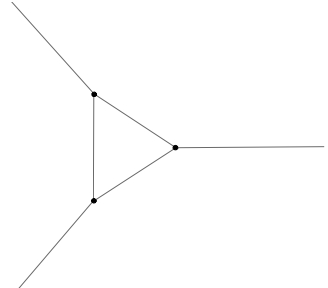
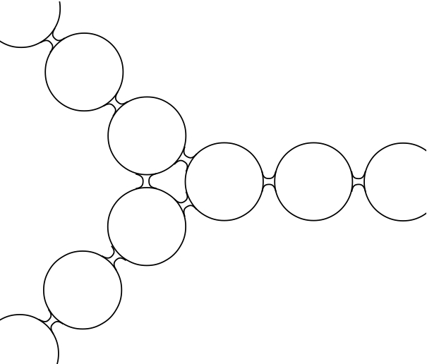
Figure 1. A balanced graph with three length-2 edges and three rays (left) and a CMC-1 surface with genus one and three Delaunay-type ends in the corresponding family (right).

2.2. Forces

The weighted graph $\Gamma$ must satisfy a balancing condition for the construction to succed. For $i\in[1,N]$:

• Let $E_{i}$ be the set of indices $j\in[1,N]$ such that the vertices ${\bf v}_{i}$ and ${\bf v}_{j}$ are connected by an edge, that is $(i,j)\in I$ or $(j,i)\in I$. For $j\in E_{i}$, let

  $${\bf u}_{ij}=\frac{{\bf v}_{j}-{\bf v}_{i}}{||{\bf v}_{j}-{\bf v}_{i}||}$$

  be the unitary vector in the direction of the edge. Finally, in case $i>j$, define $\tau_{ij}=\tau_{ji}$.

• Let $R_{i}$ be the set of indices $k\in[1,n]$ such that $r_{k}$ is a half-line issued from ${\bf v}_{i}$. For $k\in R_{i}$, let ${\bf u}_{k}$ be the unitary vector spanning the half-line $r_{k}$

We define the force ${\bf f}_{i}$ acting on the vertex ${\bf v}_{i}$ by

$${\bf f}_{i}=\sum_{j\in E_{i}}\tau_{ij}{\bf u}_{ij}+\sum_{k\in R_{i}}\tau_{k}{\bf u}_{k}$$

Definition 2.

A weighted graph $\Gamma$ is balanced if for all $i\in[1,N]$, ${\bf f}_{i}=0$.

2.3. Non-degeneracy

To apply the Implicit Function Theorem, we need to perturb our graph $\Gamma$ in order to prescribe small variations of edge-lengths and forces. The parameters available to deform $\Gamma$ are: the position of the vertices ${\bf v}_{i}$, the direction of the rays $r_{k}$ and the weights of the edges and rays. The abstract structure of the graph is fixed under this deformation (so the edges are determined by the positions of the vertices).

Definition 3.

A weighted graph $\Gamma$ is non-degenerate if the jacobian of the map

$$\left(({\bf f}_{i})_{1\leq i\leq N},(\ell_{ij})_{(i,j)\in I}\right)\in{\mathbb{R}}^{3N}\times{\mathbb{R}}^{I}$$

with respect to the parameters (vertices, rays, weights) is onto.

Remark 1.

There are plenty of interesting examples of non-degenerate graphs in [15]. Our non-degeneracy condition is slightly different from the flexibility condition of Kapouleas (Definition 1.18 in [15]). It is, however, very natural for our implicit function approach.

Remark 2.

If a weighted graph has no rays, then $\sum_{i=1}^{N}{\bf f}_{i}=0$ so it is always degenerate. We will not construct compact CMC-1 surfaces in this paper.

2.4. Main result

Theorem 1.

Assume that $\Gamma$ has even-length edges, is balanced and non-degenerate. There exists a smooth 1-parameter family of immersed CMC-1 surfaces $(M_{t})_{0<t<\epsilon}$ with the following properties:

1. $M_{t}$ converges as $t\to 0$ to $M_{0}$. The convergence is for the Hausdorf distance on compact sets of ${\mathbb{R}}^{3}$.

2. $M_{t}$ is homeomorphic to a tubular neighborhood of $\Gamma$.

3. For each $k\in[1,n]$, $M_{t}$ has a Delaunay end with weight $\simeq 8\pi t\tau_{k}$ and whose axis converges as $t\to 0$ to the ray $r_{k}$.

4. If $\Gamma$ is pre-embedded, then $M_{t}$ is embedded.

Definition 4.

Following Kapouleas (Definition 2.2 in [15]), we say that $\Gamma$ is pre-embedded if:

1. All weights are positive.

2. The distance between any two edges or rays which have no common endpoint is greater than $2$.

3. The angle between any two edges or rays with a common endpoint is greater than $60^{\circ}$.

As already said, Theorem 1 was proved using a completely different method in [15]. In the simplest case $N=1$, there is no need for Opening Nodes and Theorem 1 is proved using the DPW method in [31]. We follow the same strategy to define the DPW potential and we will use some of the results in [31].

2.5. Reduction to length-2 edges

Let $\Gamma$ be a graph with $N$ vertices and even-length edges. Assume that $\Gamma$ has an edge $e_{ij}$ of length $\ell_{ij}\geq 4$. We can define a new graph $\widetilde{\Gamma}$ as follows: insert a new vertex ${\bf v}_{N+1}$ on the edge $e_{ij}$ at distance $2$ from ${\bf v}_{i}$. Replace the edge $e_{ij}$ by the edges $[{\bf v}_{i},{\bf v}_{N+1}]$ and $[{\bf v}_{N+1},{\bf v}_{j}]$, with respective lenghts $2$ and $\ell_{ij}-2$. Assign to each new edge the weight $\tau_{ij}$. The new graph $\widetilde{\Gamma}$ is clearly balanced.

Proposition 1.

If $\Gamma$ is non-degenerate then $\widetilde{\Gamma}$ is non-degenerate. If $\Gamma$ is pre-embedded then $\widetilde{\Gamma}$ is pre-embedded.

The proof of Proposition 1 is elementary and is omitted. Thanks to Proposition 1, we can transform by induction the graph $\Gamma$ into a balanced, non-degenerate graph with length-2 edges. Therefore, it suffices to prove Theorem 1 in the case where all edges have length 2.

3. Background

3.1. Opening nodes

In this section, we recall the standard construction of opening nodes. Consider $n$ copies of the Riemann sphere $\overline{{\mathbb{C}}}={\mathbb{C}}\cup\{\infty\}$, labelled $\overline{{\mathbb{C}}}_{1},\cdots,\overline{{\mathbb{C}}}_{n}$. Consider $2m$ distinct points $p_{1},\cdots,p_{m}$, $q_{1},\cdots,q_{m}$ in the disjoint union $\overline{{\mathbb{C}}}_{1}\cup\cdots\cup\overline{{\mathbb{C}}}_{n}$. Identify $p_{i}$ with $q_{i}$ for all $i\in[1,m]$. This defines a Rieman surface with nodes which we denote $\Sigma_{0}$. (The nodes refer to the double points $p_{i}\sim q_{i}$).

To open nodes, consider local complex coordinates $v_{i}:V_{i}\stackrel{{\scriptstyle\sim}}{{\to}}D(0,\varepsilon)$ in a neighborhood of $p_{i}$ and $w_{i}:W_{i}\stackrel{{\scriptstyle\sim}}{{\to}}D(0,\varepsilon)$ in a neighborhood of $q_{i}$, with $v_{i}(p_{i})=0$ and $w_{i}(q_{i})=0$. We assume that the neighborhoods $V_{1},\cdots,V_{m},W_{1},\cdots,W_{m}$ are disjoint in $\overline{{\mathbb{C}}}_{1}\cup\cdots\cup\overline{{\mathbb{C}}}_{n}$. Consider, for each $i\in[1,m]$, a complex parameter $t_{i}$ with $|t_{i}|<\varepsilon^{2}$. If $t_{i}=0$, identify $p_{i}$ with $q_{i}$ as above. If $t_{i}\neq 0$, remove the disks $|v_{i}|\leq\frac{|t_{i}|}{\varepsilon}$ and $|w_{i}|\leq\frac{|t_{i}|}{\varepsilon}$. Identify each point $z$ in the annulus $\frac{|t_{i}|}{\varepsilon}<|v_{i}|<\varepsilon$ with the point $z^{\prime}$ in the annulus $\frac{|t_{i}|}{\varepsilon}<|w_{i}|<\varepsilon$ such that

$$v_{i}(z)w_{i}(z^{\prime})=t_{i}.$$

(In particular, the circle $|v_{i}|=|t_{i}|^{1/2}$ is identified with the circle $|w_{i}|=|t_{i}|^{1/2}$, with the reverse orientation.) This creates a Riemann surface (possibly with nodes) which we denote $\Sigma_{{\bf t}}$, where ${\bf t}=(t_{1},\cdots,t_{n})$. If $t_{i}\neq 0$, we can use $v_{i}$ and $w_{i}$ as local coordinates in $\Sigma_{{\bf t}}$, and the change of coordinate $\psi_{i}=w_{i}\circ v_{i}^{-1}$ is given by $\psi_{i}(z)=\frac{t_{i}}{z}$. When all $t_{i}$ are non-zero, $\Sigma_{{\bf t}}$ is a genuine compact Riemann surface. If $\Sigma_{0}$ is connected, its genus is $m-n+1$.

One can define meromorphic 1-forms on a compact Riemann surface by prescribing principal parts and periods. In the case of opening nodes, this can be formulated as follows.

Definition 5.

Let $r_{1},\cdots,r_{k}$ be points in $\Sigma_{0}$, distinct from the nodes. A meromorphic regular differential $\omega_{0}$ on $\Sigma_{0}$ with poles at $r_{1},\cdots,r_{k}$ is a meromorphic 1-form on the disjoint union $\overline{{\mathbb{C}}}_{1}\cup\cdots\cup\overline{{\mathbb{C}}}_{n}$ with poles at $r_{1},\cdots,r_{k}$ and simple poles at $p_{i},q_{i}$ for $i\in[1,m]$ such that the residues at $p_{i}$ and $q_{i}$ are opposite.

In the case $k=0$, $\omega_{0}$ is called a holomorphic regular differential, or simply a regular differential.

Theorem 2.

Given a meromorphic regular differential $\omega_{0}$ on $\Sigma_{0}$, for ${\bf t}$ in a neighborhood of $0$, there exists a unique meromorphic regular differential $\omega_{{\bf t}}$ on $\Sigma_{{\bf t}}$, such that:

1. For $i\in[1,m]$,

   $$\int_{\gamma_{i}}\omega_{{\bf t}}=\int_{\gamma_{i}}\omega_{0}$$

   where $\gamma_{i}$ denotes the circle $|v_{i}|=\varepsilon$.

2. For $i\in[1,k]$, $\omega_{{\bf t}}-\omega_{0}$ extends holomorphically at $r_{i}$.

Moreover, $\omega_{{\bf t}}-\omega_{0}$ depends holomorphically on ${\bf t}$ on compact subsets of $\Sigma_{0}$ minus the nodes.

As indicated by the notation, when ${\bf t}=0$, $\omega_{{\bf t}}$ is equal to the given meromorphic regular differential $\omega_{0}$. In case all $t_{i}$ are non-zero, $\omega_{\bf t}$ is of course a genuine meromorphic 1-form on $\Sigma_{{\bf t}}$. Regarding the last point, a compact subset of $\Sigma_{0}$ minus the nodes is included in $\Sigma_{{\bf t}}$ for ${\bf t}$ small enough.

Theorem 2 was first proved by Fay [5] in the case of holomorphic regular differentials, using sheaf theory. This was extended to the case of meromorphic differentials with simple poles by Masur [21]. An elementary proof of the general case is given in [29] using an Implicit Function Theorem argument.

Remark 3.

When all $t_{i}$ are non-zero, the existence of the meromorphic 1-form $\omega_{{\bf t}}$ on $\Sigma_{{\bf t}}$ follows from the standard theory of compact Riemann surfaces. The content of Theorem 2 is really that the limit of $\omega_{{\bf t}}$ as ${\bf t}\to 0$ exists and equals $\omega_{0}$.

An important point for our construction is that $\omega_{0}$ can be explicitely computed, since meromorphic 1-forms on the Riemann sphere are rational fractions. In fact, we can also compute the partial derivatives of $\omega_{{\bf t}}$ with respect to $t_{i}$ at ${\bf t}=0$, to any order. In this paper, we only need the first order derivative:

Theorem 3.

In compact subsets of $\Sigma_{0}$ minus the nodes, the partial derivative $\frac{\partial\omega_{{\bf t}}}{\partial t_{i}}|_{{\bf t}=0}$ is equal to the unique meromorphic differential on the disjoint union $\overline{{\mathbb{C}}}_{1}\cup\cdots\cup\overline{{\mathbb{C}}}_{n}$ which has only two double poles at $p_{i}$ and $q_{i}$, with principal parts

$$\frac{-dv_{i}}{v_{i}^{2}}{\,\rm Res}_{q_{i}}\left(\frac{\omega_{0}}{w_{i}}\right)\qquad\mbox{ at $p_{i}$}$$

$$\frac{-dw_{i}}{w_{i}^{2}}{\,\rm Res}_{p_{i}}\left(\frac{\omega_{0}}{v_{i}}\right)\qquad\mbox{ at $q_{i}$}$$

This is proven in [28], Lemma 3. See also [29], Remark 5.6.

3.2. The DPW method

In this section, we recall standard notations and results used in the DPW method in the “untwisted” setting. For a comprehensive introduction to the DPW method, we suggest [7].

3.2.1. Loop groups

We use blackboard letters for domains in the $\lambda$-plane. For $\rho>1$, we denote:

• ${\mathbb{S}}^{1}$ the unit circle $\{\lambda\in{\mathbb{C}}:|\lambda|=1\}$,

• ${\mathbb{D}}$ the unit disk $\{\lambda\in{\mathbb{C}}:|\lambda|<1\}$,

• ${\mathbb{D}}_{\rho}$ the disk $\{\lambda\in{\mathbb{C}}:|\lambda|<\rho\}$,

• ${\mathbb{D}}_{\rho}^{*}$ the punctured disk ${\mathbb{D}}_{\rho}\setminus\{0\}$,

• ${\mathbb{A}}_{\rho}$ the annulus $\{\lambda\in{\mathbb{C}}:\rho^{-1}<|\lambda|<\rho\}$.

A loop is a smooth map from the unit circle to a matrix Lie group.

• If $G$ is a matrix Lie group (respectively a Lie algebra), $\Lambda G$ denotes the group (respectively the algebra) of smooth maps $\Phi:{\mathbb{S}}^{1}\to G$.

• $\Lambda_{+}SL(2,{\mathbb{C}})\subset\Lambda SL(2,{\mathbb{C}})$ is the subgroup of smooth maps $B:{\mathbb{S}}^{1}\to SL(2,{\mathbb{C}})$ which extend holomorphically to the unit disk ${\mathbb{D}}$.

• $\Lambda_{+}^{{\mathbb{R}}}SL(2,{\mathbb{C}})$ is the set of $B\in\Lambda_{+}SL(2,{\mathbb{C}})$ such that $B(0)$ is upper triangular with real elements on the diagonal.

Theorem 4 (Iwasawa decomposition).

The multiplication $\Lambda SU(2)\times\Lambda_{+}^{{\mathbb{R}}}SL(2,{\mathbb{C}})\to\Lambda SL(2,{\mathbb{C}})$ is a diffeomorphism. The unique splitting of an element $\Phi\in\Lambda SL(2,{\mathbb{C}})$ as $\Phi=FB$ with $F\in\Lambda SU(2)$ and $B\in\Lambda_{+}^{{\mathbb{R}}}SL(2,{\mathbb{C}})$ is called Iwasawa decomposition. $F$ is called the unitary factor of $\Phi$ and denoted $\mbox{Uni}(\Phi)$. $B$ is called the positive factor and denoted $\mbox{Pos}(\Phi)$.

3.2.2. The matrix model of ${\mathbb{R}}^{3}$

In the DPW method, one identifies ${\mathbb{R}}^{3}$ with the Lie algebra ${\mathfrak{s}u}(2)$ by

$$x=(x_{1},x_{2},x_{3})\in{\mathbb{R}}^{3}\longleftrightarrow X=\frac{-{\rm i}}{2}\left(\begin{array}[]{cc}-x_{3}&x_{1}+{\rm i}x_{2}\\ x_{1}-{\rm i}x_{2}&x_{3}\end{array}\right)\in\mathfrak{su}(2)$$

The group $SU(2)$ acts as linear isometries on ${\mathfrak{s}u}(2)$ by $H\cdot X=HXH^{-1}$.

3.2.3. The recipe

The input data for the DPW method is a quadruple $(\Sigma,\xi,z_{0},\Phi_{0})$ where:

• $\Sigma$ is a Riemann surface.

• $\xi$ is a $\Lambda{\mathfrak{s}l}(2,{\mathbb{C}})$-valued holomorphic 1-form on $\Sigma$ called the DPW potential. More precisely,

  $$\xi(z,\lambda)=\left(\begin{array}[]{cc}\alpha(z,\lambda)&\lambda^{-1}\beta(z,\lambda)\\ \gamma(z,\lambda)&-\alpha(z,\lambda)\end{array}\right)$$

  where $\alpha$, $\beta$, $\gamma$ are holomorphic 1-forms on $\Sigma$ with respect to the $z$ variable and depend holomorphically on $\lambda$ in the disk ${\mathbb{D}}_{\rho}$ for some $\rho>1$.

• $z_{0}\in\Sigma$ is a base point.

• $\phi_{0}\in\Lambda SL(2,{\mathbb{C}})$ is an initial condition.

Given this data, the DPW method is the following procedure. Let $\widetilde{\Sigma}$ be the universal cover of $\Sigma$ and $\widetilde{z}_{0}\in\widetilde{\Sigma}$ be an arbitrary element in the fiber of $z_{0}$.

1. Solve the Cauchy problem on $\widetilde{\Sigma}$:

   $$\left\{\begin{array}[]{l}d\Phi(z,\lambda)=\Phi(z,\lambda)\xi(z,\lambda)\\ \Phi(\widetilde{z}_{0},\lambda)=\phi_{0}(\lambda)\end{array}\right.$$ (1)

   to obtain a solution $\Phi:\widetilde{\Sigma}\to\Lambda SL(2,{\mathbb{C}})$. (The lift of $\xi$ to $\widetilde{\Sigma}$ is still denoted $\xi$.)

2. Compute, for $z\in\widetilde{\Sigma}$, the Iwasawa decomposition $(F(z,\cdot),B(z,\cdot))$ of $\Phi(z,\cdot)$.

3. Define $f:\widetilde{\Sigma}\to{\mathfrak{s}u}(2)\sim{\mathbb{R}}^{3}$ by the Sym-Bobenko formula:

   $$f(z)={\rm i}\frac{\partial F}{\partial\lambda}(z,1)F(z,1)^{-1}=:\mbox{Sym}(F(z,\cdot)).$$ (2)

   Then $f$ is a CMC-1 (banched) conformal immersion. Its Gauss map is given by

   $$N(z)=\frac{-{\rm i}}{2}F(z,1)\left(\begin{array}[]{cc}1&0\\ 0&-1\end{array}\right)F(z,1)^{-1}=:\mbox{Nor}(F(z,\cdot))$$ (3)

   In term of local conformal coordinates $z=x+{\rm i}y$, the derivatives of $f$ are given by:

   $$\frac{\partial f}{\partial x}(z)=\frac{-{\rm i}}{2}\;\mu(z)F(z,1)\left(\begin{array}[]{cc}0&1\\ 1&0\end{array}\right)F(z,1)^{-1}$$ (4)

   $$\frac{\partial f}{\partial y}(z)=\frac{-{\rm i}}{2}\;\mu(z)F(z,1)\left(\begin{array}[]{cc}0&-{\rm i}\\ {\rm i}&0\end{array}\right)F(z,1)^{-1}$$ (5)

   where $\mu$ is the conformal factor of the immersion.

   We will use the following notation: if $u$ is a smooth function of $\lambda$ on the unit circle, we denote $u^{0}$ the coefficient of $\lambda^{0}$ in its Fourier decomposition and $u^{(-1)}$ the coefficient of $\lambda^{-1}$. The elements of $\xi$ are denoted $\xi_{ij}$ for $1\leq i,j\leq 2$. If the potential $\xi_{t}$ depends on some parameter $t$, its elements are denoted $\xi_{t;ij}$, and the same conventions apply to all matrices. With these notations, the conformal metric induced by the immersion is given by

   $$ds=\mu|dz|=2(B_{11}^{0})^{2}|\xi_{12}^{(-1)}|.$$ (6)

Remark 4.

What the DPW method actually does is construct the moving frame $(\mu^{-1}\frac{\partial f}{\partial x},\mu^{-1}\frac{\partial f}{\partial y},N)$, which is encoded in the unitary matrix $F(z,1)$. The Sym-Bobenko formula is a magical trick to recover the immersion $f$ directly.

3.2.4. The Monodromy Problem

Assume that $\Sigma$ is not simply connected so its universal cover $\widetilde{\Sigma}$ is not trivial. Let $\mbox{Deck}(\widetilde{\Sigma}/\Sigma)$ be the group of fiber-preserving diffeomorphisms of $\widetilde{\Sigma}$. For $\sigma\in\mbox{Deck}(\widetilde{\Sigma}/\Sigma)$, let

$${\mathcal{M}}(\Phi,\sigma)(\lambda)=\Phi(\sigma(z),\lambda)\Phi(z,\lambda)^{-1}$$

be the monodromy of $\Phi$ with respect to $\sigma$, which is independent of $z\in\widetilde{\Sigma}$. The standard condition which ensures that the immersion $f$ descends to a well defined immersion on $\Sigma$ is the following system of equations, called the Monodromy Problem:

$$\forall\sigma\in\mbox{Deck}(\widetilde{\Sigma}/\Sigma)\quad\left\{\begin{array}[]{lc}{\mathcal{M}}(\Phi,\sigma)\in\Lambda SU(2)&(i)\\ {\mathcal{M}}(\Phi,\sigma)(1)=\pm I_{2}&(ii)\\ \frac{\partial}{\partial\lambda}{\mathcal{M}}(\Phi,\sigma)(1)=0&(iii)\end{array}\right.$$ (7)

3.2.5. Gauging

Definition 6.

A gauge on $\Sigma$ is a map $G:\Sigma\to\Lambda_{+}SL(2,{\mathbb{C}})$ such that $G(z,\lambda)$ depends holomorphically on $z\in\Sigma$ and $\lambda\in{\mathbb{D}}_{\rho}$, and $G(z,0)$ is upper triangular (with no restriction on its diagonal elements).

Let $\Phi$ be a solution of $d\Phi=\Phi\xi$ and $G$ be a gauge. Let ${\widehat{\Phi}}=\Phi\times G$. It is standard that $\Phi$ and ${\widehat{\Phi}}$ define the same immersion $f$. The gauged potential is

$${\widehat{\xi}}:={\widehat{\Phi}}^{-1}d{\widehat{\Phi}}=G^{-1}\xi G+G^{-1}dG$$

and is denoted $\xi\cdot G$, the dot denoting the action of the gauge group on the potential. Gauging does not change the Monodromy of $\Phi$ (provided $G$ is well defined in $\Sigma$):

$${\mathcal{M}}(\Phi\times G,\sigma)=\Phi(\sigma(z))G(\sigma(z))G(z)^{-1}\Phi(z)^{-1}={\mathcal{M}}(\Phi,\sigma).$$

We will need the following standard result, which is an easy computation:

Proposition 2.

Let $G(z,\lambda)$ be a gauge and ${\widehat{\xi}}=\xi\cdot G$. Then (using the notations introduced at the end of Section 3.2.3)

$${\widehat{\xi}}_{12}^{\,(-1)}=(G_{22}^{0})^{2}\xi_{12}^{(-1)}$$

$${\widehat{\xi}}_{21}^{\,0}=(G_{11}^{0})^{2}\xi_{21}^{0}.$$

3.2.6. The Regularity Problem

Definition 7.

We say that $\xi$ is regular at $z\in\Sigma$ if $\xi_{12}^{(-1)}(z)\neq 0$.

In view of Equation (6), this ensures that the immersion $f$ is unbranched at $z$. In many cases, $\Sigma$ is a compact Riemann surface $\overline{\Sigma}$ minus a finite number of points, and the potential $\xi$ extends meromorphically to $\overline{\Sigma}$.

Definition 8.

Let $p\in\overline{\Sigma}$ be a pole of $\xi$. We say that $p$ is a removable singularity if there exists a local gauge $G$ in a neighborhood of $p$ such that $\xi\cdot G$ extends holomorphically at $p$.

This ensures that the immersion $f$ extends analytically at $p$.

In many cases, the meromorphic 1-form $\xi_{12}^{(-1)}$ has zeros in $\overline{\Sigma}$. (This is always the case if the genus of $\overline{\Sigma}$ is greater than one). If $p$ is a zero of of $\xi_{12}^{(-1)}$ and we want $f$ to be unbranched at $p$, then $\xi$ must have a pole at $p$, $p$ must be a removable singularity and $\xi\cdot G$ must be regular at $p$.

3.2.7. Dressing and isometries

Let $H\in\Lambda SL(2,{\mathbb{C}})$. Let $\Phi(z,\lambda)$ be a solution of $d\Phi=\Phi\xi$. Then ${\widetilde{\Phi}}=H\Phi$ is a solution of $d{\widetilde{\Phi}}={\widetilde{\Phi}}\xi$. This is called “dressing” and amounts to change the initial value $\phi_{0}$. In general, the effect of dressing on the immersion $f$ is not explicit. However if $H\in\Lambda SU(2)$ then by uniqueness in the Iwasawa decomposition we have

$${\widetilde{F}}(z,\lambda)=H(\lambda)F(z,\lambda)$$

and by the Sym-Bobenko formula,

$${\widetilde{f}}(z)=H(1)f(z)H(1)^{-1}+{\rm i}\frac{\partial H}{\partial\lambda}(1)H(1)^{-1}.$$ (8)

Hence ${\widetilde{f}}=H\cdot f$ where the action of $\Lambda SU(2)$ as rigid motions of ${\mathfrak{s}u}(2)\sim{\mathbb{R}}^{3}$ is given by

$$H\cdot X=H(1)XH(1)^{-1}+{\rm i}\frac{\partial H}{\partial\lambda}(1)H(1)^{-1}.$$ (9)

3.2.8. Duality

Let $\xi$ be a DPW potential, $\Phi$ a solution of Problem (1) and

$$H(\lambda)=\left(\begin{array}[]{cc}0&\frac{{\rm i}}{\sqrt{\lambda}}\\ {\rm i}\sqrt{\lambda}&0\end{array}\right).$$

I define the dual potential ${\widecheck{\xi}}$ and its dual solution $\widecheck{\Phi}$ (the terminology is not standard) by

$${\widecheck{\xi}}=H^{-1}\xi H\quad\mbox{ and }\quad\widecheck{\Phi}=H^{-1}\Phi H$$

which are both independent of the choice of the square root in $H$, so are well defined. Explicitely,

$$H^{-1}\left(\begin{array}[]{cc}\alpha&\lambda^{-1}\beta\\ \gamma&-\alpha\end{array}\right)H=\left(\begin{array}[]{cc}-\alpha&\lambda^{-1}\gamma\\ \beta&\alpha\end{array}\right)$$

so we see that duality essentially exchanges $\beta$ and $\gamma$. We will take advantage of this to prove Corollary 1 in Appendix A. Duality changes the immersion in the following explicit way: it is easy to see that if $(F,B)$ is the Iwasawa decomposition of $\Phi$, then the Iwasawa decomposition of $\widecheck{\Phi}$ is

$$\widecheck{F}:=\mbox{Uni}(\widecheck{\Phi})=H^{-1}FH\quad\mbox{ and }\quad\widecheck{B}:=\mbox{Pos}(\widecheck{\Phi})=H^{-1}BH.$$

If $f=\mbox{Sym}(\mbox{Uni}(f))$, the Sym-Bobenko formula gives after an easy computation:

$$\widecheck{f}(z):=\mbox{Sym}(\mbox{Uni}(\widecheck{f}))=H(1)^{-1}\left[\frac{-{\rm i}}{2}\left(\begin{array}[]{cc}-1&0\\ 0&1\end{array}\right)+f(z)+N(z)\right]H(1).$$

In other words, in euclidean coordinates,

$$\widecheck{f}(z)=\sigma(f(z)+N(z)+(0,0,1))\quad\mbox{ where }\quad\sigma(x_{1},x_{2},x_{3})=(x_{1},-x_{2},-x_{3}).$$

So up to a rigid motion, the dual (branched) immersion $\widecheck{f}$ is the parallel surface at distance one to $f$. Formula (3) gives the Gauss map of $\widecheck{f}$:

$$\widecheck{N}(z)=-\sigma(N(z)).$$

Remark 5.

In this paper, we use the notations ${\widetilde{\xi}}$, ${\widehat{\xi}}$ and ${\widecheck{\xi}}$ to denote various transformations undergone by the potential $\xi$, including gauging, rescaling, pullback and dressing (so ${\widetilde{\xi}}$ does not necessarily mean dressing and ${\widecheck{\xi}}$ does not necessarily mean dual). These notations will always be consistently applied to all quantities derived from the potential: ${\widetilde{\Phi}}$, ${\widetilde{F}}$, ${\widetilde{B}}$, ${\widetilde{f}}$ are derived from ${\widetilde{\xi}}$.

3.2.9. The standard sphere

We denote $\xi^{S}$ the standard DPW potential for the sphere in ${\mathbb{C}}$:

$$\xi^{S}(z,\lambda)=\left(\begin{array}[]{cc}0&\lambda^{-1}\\ 0&0\end{array}\right)dz.$$

The following computation shows that $\infty$ is a regular removable singularity:

$$\xi^{S}\cdot\left(\begin{array}[]{cc}z&0\\ -\lambda&z^{-1}\end{array}\right)=\left(\begin{array}[]{cc}0&\lambda^{-1}\\ 0&0\end{array}\right)\frac{dz}{z^{2}}.$$

Let $\Phi^{S}$ the solution of $d\Phi^{S}=\Phi^{S}\xi^{S}$ with initial condition $\Phi^{S}(0,\lambda)=I_{2}$ in ${\mathbb{C}}$:

$$\Phi^{S}(z,\lambda)=\left(\begin{array}[]{cc}1&\lambda^{-1}z\\ 0&1\end{array}\right).$$

The Iwasawa decomposition of $\Phi^{S}(z)$ is explicitely given by

$$F^{S}(z,\lambda)=\mbox{Uni}(\Phi^{S}(z,\lambda))=\frac{1}{\sqrt{1+|z|^{2}}}\left(\begin{array}[]{cc}1&\lambda^{-1}z\\ -\lambda\overline{z}&1\end{array}\right)$$

$$B^{S}(z,\lambda)=\mbox{Pos}(\Phi^{S}(z,\lambda))=\frac{1}{\sqrt{1+|z|^{2}}}\left(\begin{array}[]{cc}1&0\\ \lambda\overline{z}&1+|z|^{2}\end{array}\right).$$

The Sym-Bobenko formula gives

$$f^{S}(z)=\frac{1}{1+|z|^{2}}\left(2{\,\rm Re}(z),2{\,\rm Im}(z),-2|z|^{2}\right)=(0,0,-1)+\pi_{S}^{-1}(z)$$

$$N^{S}(z)=\frac{-1}{1+|z|^{2}}\left(2{\,\rm Re}(z),2{\,\rm Im}(z),1-|z|^{2}\right)=-\pi_{S}^{-1}(z)$$

where $\pi_{S}:{\mathbb{S}}^{2}\to{\mathbb{C}}\cup\{\infty\}$ is the stereographic projection from the south pole.

3.2.10. The infinitesimal catenoid

We denote $\xi^{C}$ the dual potential to $\xi^{S}$:

$$\xi^{C}(z,\lambda)=\left(\begin{array}[]{cc}0&0\\ 1&0\end{array}\right)dz$$

The dual solution is

$$\Phi^{C}(z,\lambda)=\left(\begin{array}[]{cc}1&0\\ z&1\end{array}\right)$$

Its Iwasawa decomposition is the standard QR decomposition (from which we could derive the Iwasawa decomposition of $\Phi^{S}$ by duality):

$$F^{C}(z,\lambda)=\mbox{Uni}(\Phi^{C}(z,\lambda))=\frac{1}{\sqrt{1+|z|^{2}}}\left(\begin{array}[]{cc}1&-\overline{z}\\ z&1\end{array}\right)$$

$$B^{C}(z,\lambda)=\mbox{Pos}(\Phi^{C}(z,\lambda))=\frac{1}{\sqrt{1+|z|^{2}}}\left(\begin{array}[]{cc}1+|z|^{2}&\overline{z}\\ 0&1\end{array}\right)$$

Since $F^{C}(z,\lambda)$ does not depend on $\lambda$, the Sym-Bobenko formula gives $f^{C}\equiv 0$: the immersion degenerates into a point, as expected by duality since the parallel surface at distance one to a unit sphere degenerates into its center. The normal is still well defined and is given by:

$$N^{C}(z)=\frac{1}{1+|z|^{2}}\left(2{\,\rm Re}(z),-2{\,\rm Im}(z),|z|^{2}-1\right).$$

We will use this potential to model catenoidal necks. (The catenoid is of course not a CMC-1 surface: it is a minimal surface.)

3.3. Principal solution

We will formulate the Monodromy Problem using the notion of principal solution (see Chapter 3.4 in [26]). Let $\Sigma$ be a Riemann surface, $\xi$ a matrix valued holomorphic 1-form on $\Sigma$ and $\gamma:[0,1]\to\Sigma$ a path (not necessarily closed). The principal solution of $\xi$ with respect to $\gamma$, denoted ${\mathcal{P}}(\xi,\gamma)$ is the value at $\gamma(1)$ of the analytical continuation along $\gamma$ of the solution $\Phi$ of $d\Phi=\Phi\xi$ with initial condition $\Phi(\gamma(0))=I_{2}$. More precisely, let $\widetilde{\Sigma}$ be the universal cover of $\Sigma$ and ${\widetilde{\gamma}}:[0,1]\to\widetilde{\Sigma}$ be an arbitrary lift of $\gamma$. Let $\Phi$ be the solution on $\widetilde{\Sigma}$ of $d\Phi=\Phi\xi$ with initial condition $\Phi({\widetilde{\gamma}}(0))=I_{2}$. Then $\Phi({\widetilde{\gamma}}(1))$ does not depend on the choice of the lift ${\widetilde{\gamma}}$ and is denoted ${\mathcal{P}}(\xi,\gamma)$. Equivalently, we can define ${\mathcal{P}}(\xi,\gamma)$ as follows: let $Y$ be the solution on $[0,1]$ of the Cauchy Problem

$$\left\{\begin{array}[]{l}Y^{\prime}(s)=Y(s)\xi(\gamma(s))\gamma^{\prime}(s)\\ Y(0)=I_{2}\end{array}\right.$$

Then ${\mathcal{P}}(\xi,\gamma)=Y(1)$. (The relation between the two definitions is $Y(s)=\Phi({\widetilde{\gamma}}(s))$.)

The principal solution has the following properties, which follow easily from its definition:

1. ${\mathcal{P}}(\xi,\gamma)$ only depends on the homotopy class of $\gamma$.

2. The principal solution is a morphism for the product of paths: If $\gamma_{1}$ and $\gamma_{2}$ are two paths such that $\gamma_{1}(1)=\gamma_{2}(0)$ then

   $${\mathcal{P}}(\xi,\gamma_{1}\gamma_{2})={\mathcal{P}}(\xi,\gamma_{1}){\mathcal{P}}(\xi,\gamma_{2}).$$ (10)

3. If $\psi:\Sigma_{1}\to\Sigma_{2}$ is a differentiable map, $\xi$ is a matrix-valued 1-form on $\Sigma_{2}$ and $\gamma$ is a path in $\Sigma_{1}$, then

   $${\mathcal{P}}(\psi^{*}\xi,\gamma)={\mathcal{P}}(\xi,\psi\circ\gamma).$$ (11)

We have the following formula to compute the derivative of the principal solution:

Proposition 3.

Let $\xi_{t}$ be a family of holomorphic matrix-valued 1-forms on a Riemann surface $\Sigma$, depending $C^{1}$ on some parameter $t$. Let $\gamma$ be a path in $\Sigma$ and ${\widetilde{\gamma}}$ an arbitrary lift of $\gamma$ to the universal cover $\widetilde{\Sigma}$. Let $\Phi_{t}$ be the solution of $d\Phi_{t}=\Phi_{t}\xi_{t}$ in $\widetilde{\Sigma}$ with initial condition $\Phi_{t}({\widetilde{\gamma}}(0))=I_{2}$. Then

$$\frac{d}{dt}{\mathcal{P}}(\xi_{t},\gamma)=\int_{{\widetilde{\gamma}}}\Phi_{t}\frac{\partial\xi_{t}}{\partial t}\Phi_{t}^{-1}\times{\mathcal{P}}(\xi_{t},\gamma).$$

This is proven in Appendix A of [31]. (In [31], this result is formulated in terms of monodromy so we assume that $\gamma$ is a closed curve, but this is not used in the proof.)

Remark 6.

If $\xi$ is holomorphic in a simply connected domain $\Omega$ and $z_{1}$ and $z_{2}$ are two points in $\Omega$, then ${\mathcal{P}}(\xi,\gamma)$ does not depend on the choice of the path $\gamma$ from $z_{1}$ to $z_{2}$ so we will sometimes denote it ${\mathcal{P}}(\xi,z_{1},z_{2})$.

Returning to the DPW method, we now formulate the Monodromy Problem in terms of the principal solution. The group $\mbox{Deck}(\widetilde{\Sigma}/\Sigma)$ is isomorphic to the fundamental group $\pi_{1}(\Sigma,z_{0})$ (Theorem 5.6 in [6]): for $\sigma\in\mbox{Deck}(\widetilde{\Sigma}/\Sigma)$, let ${\widetilde{\gamma}}$ be an arbitrary path in $\widetilde{\Sigma}$ from $\widetilde{z}_{0}$ to $\sigma(\widetilde{z}_{0})$ and $\gamma\in\pi_{1}(\Sigma,z_{0})$ be the projection of ${\widetilde{\gamma}}$. Then $\gamma$ is the image of $\sigma$. (This isomorphism is not canonical: it depends on the choice of $\widetilde{z}_{0}$.) The monodromy of $\Phi$ with respect to $\sigma$ and the principal solution of $\xi$ with respect to $\gamma$ are related by

$${\mathcal{M}}(\Phi,\sigma)(\lambda)=\Phi({\widetilde{\gamma}}(1),\lambda)\Phi({\widetilde{\gamma}}(0),\lambda)^{-1}=\Phi(\widetilde{z}_{0},\lambda){\mathcal{P}}(\xi,\gamma)(\lambda)\Phi(\widetilde{z}_{0},\lambda)^{-1}.$$ (12)

In particular, if $\Phi(\widetilde{z}_{0},\lambda)=I_{2}$ (which will be the case in this paper), the Monodromy Problem (7) is equivalent to the following problem (which we still call the Monodromy Problem):

$$\forall\gamma\in\pi_{1}(\Sigma,z_{0})\quad\left\{\begin{array}[]{lc}{\mathcal{P}}(\xi,\gamma)\in\Lambda SU(2)&(i)\\ {\mathcal{P}}(\xi,\gamma)(1)=\pm I_{2}&(ii)\\ \frac{\partial}{\partial\lambda}{\mathcal{P}}(\xi,\gamma)(1)=0&(iii)\end{array}\right.$$ (13)

We conclude this section with a standard result which we will use to study the restriction of the immersion $f$ to a subdomain $\Omega$ of $\Sigma$:

Proposition 4.

Let $p:\widetilde{\Sigma}\to\Sigma$ be the universal covering map of $\Sigma$. Let $\Omega$ be a connected domain in $\Sigma$ and $z_{0}\in\Omega$. Let $\widetilde{z}_{0}\in p^{-1}(z_{0})$ and ${\widetilde{\Omega}}$ be the component of $p^{-1}(\Omega)$ containing $\widetilde{z}_{0}$. Assume that the inclusion $i:\Omega\to\Sigma$ induces an injective morphism $i_{*}:\pi_{1}(\Omega,z_{0})\to\pi_{1}(\Sigma,z_{0})$. Then ${\widetilde{\Omega}}$ is simply connected, so the restriction $p:{\widetilde{\Omega}}\to\Omega$ is a universal covering map of $\Omega$.

3.4. Functional spaces

In this section, we introduce functional spaces for functions of the variable $\lambda\in{\mathbb{S}}^{1}$.

3.4.1. The Banach algebra ${\mathcal{W}}$

We decompose a smooth function $f:{\mathbb{S}}^{1}\to{\mathbb{C}}$ in Fourier series

$$f(\lambda)=\sum_{i\in{\mathbb{Z}}}c_{i}\lambda^{i}$$

Fix some $\rho>1$ and define

$$||f||=\sum_{i\in{\mathbb{Z}}}|c_{i}|\rho^{|i|}$$

Let ${\mathcal{W}}$ be the space of functions $f$ with finite norm. This is a Banach algebra (classically called the Wiener algebra when $\rho=1$). Functions in ${\mathcal{W}}$ extend holomorphically to the annulus ${\mathbb{A}}_{\rho}$ and satisfy $|f(\lambda)|\leq||f||$ for all $\lambda\in{\mathbb{A}}_{\rho}$.

We define ${\mathcal{W}}^{{\geq 0}}$, ${\mathcal{W}}^{{+}}$, ${\mathcal{W}}^{{\leq 0}}$ and ${\mathcal{W}}^{{-}}$ as the subspaces of functions $f$ such that $c_{i}=0$ for $i<0$, $i\leq 0$, $i>0$ and $i\geq 0$, respectively. Functions in ${\mathcal{W}}^{{\geq 0}}$ extend holomorphically to the disk ${\mathbb{D}}_{\rho}$ and satisfy $|f(\lambda)|\leq||f||$ for all $\lambda\in{\mathbb{D}}_{\rho}$. We also write ${\mathcal{W}}^{0}$ for the subspace of constant functions, so we have a direct sum ${\mathcal{W}}={\mathcal{W}}^{{-}}\oplus{\mathcal{W}}^{0}\oplus{\mathcal{W}}^{{+}}$. A function $f$ will be decomposed as $f=f^{{-}}+f^{0}+f^{{+}}$, where $f^{0}=c_{0}$. We also denote $f^{(-1)}=c_{-1}$ the coefficient of $\lambda^{-1}$ in the Fourier series of $f$.

We define the star operator by

$$f^{*}(\lambda)=\overline{f\left(\frac{1}{\overline{\lambda}}\right)}=\sum_{i\in{\mathbb{Z}}}\overline{c_{-i}}\lambda^{i}$$

The involution $f\mapsto f^{*}$ exchanges ${\mathcal{W}}^{{\geq 0}}$ and ${\mathcal{W}}^{{\leq 0}}$. We have $\lambda^{*}=\lambda^{-1}$ and $c^{*}=\overline{c}$ if $c$ is a constant.

3.4.2. Linear operators

The value $\lambda=1$ plays a special role in the DPW method because the Sym-Bobenko formula is evaluated at $\lambda=1$. We shall need the following result in the case $\mu=1$:

Proposition 5.

For $\mu\in{\mathbb{C}}$, define

$${\mathcal{L}}_{\mu}(f)(\lambda)=\frac{f(\lambda)-f(\mu)}{\lambda-\mu}.$$

1. If $\mu\in{\mathbb{D}}_{\rho}$, then ${\mathcal{L}}_{\mu}:{\mathcal{W}}^{\geq 0}\to{\mathcal{W}}^{\geq 0}$ is a bounded operator with norm at most $\frac{1}{\rho-|\mu|}$. Consequently, any $f\in{\mathcal{W}}^{{\geq 0}}$ can be decomposed in a unique way as

   $$f(\lambda)=f(\mu)+(\lambda-\mu){\widetilde{f}}(\lambda)\quad\mbox{ with }{\widetilde{f}}={\mathcal{L}}(f)\in{\mathcal{W}}^{\geq 0}.$$

2. If $\mu\in{\mathbb{A}}_{\rho}$, then ${\mathcal{L}}_{\mu}:{\mathcal{W}}\to{\mathcal{W}}$ is a bounded operator with norm at most $\max\{\frac{1}{\rho-|\mu|},\frac{1}{|\mu|-\rho^{-1}}\}$.

Proof:

1. Let $f\in{\mathcal{W}}^{\geq 0}$. Writing $f(\lambda)=\sum_{i=0}^{\infty}c_{i}\lambda^{i}$, we have:

   $${\mathcal{L}}_{\mu}(f)(\lambda)=\sum_{i=0}^{\infty}c_{i}\frac{\lambda^{i}-\mu^{i}}{\lambda-\mu}=\sum_{i=0}^{\infty}c_{i}\sum_{j=0}^{i-1}\lambda^{j}\mu^{i-1-j}$$

   $$||{\mathcal{L}}_{\mu}(f)||\leq\sum_{i=0}^{\infty}|c_{i}|\sum_{j=0}^{i-1}\rho^{j}|\mu|^{i-1-j}=\sum_{i=0}^{\infty}|c_{i}|\frac{\rho^{i}-|\mu|^{i}}{\rho-|\mu|}\leq\sum_{i=0}^{\infty}\frac{|c_{i}|\rho^{i}}{\rho-|\mu|}=\frac{||f||}{\rho-|\mu|}.$$

   Hence ${\mathcal{L}}_{\mu}(f)\in{\mathcal{W}}^{{\geq 0}}$ and $|||{\mathcal{L}}_{\mu}|||\leq\frac{1}{\rho-|\mu|}$.

2. Let $f\in{\mathcal{W}}^{\leq 0}$. Then $f^{*}\in{\mathcal{W}}^{\geq 0}$ and

   $${\mathcal{L}}_{\mu}(f)^{*}(\lambda)=\frac{f^{*}(\lambda)-\overline{f(\mu)}}{\lambda^{-1}-\overline{\mu}}=-\frac{\lambda}{\overline{\mu}}\left(\frac{f^{*}(\lambda)-f^{*}(\frac{1}{\overline{\mu}})}{\lambda-\frac{1}{\overline{\mu}}}\right)=-\frac{\lambda}{\overline{\mu}}{\mathcal{L}}_{1/\overline{\mu}}(f^{*})(\lambda).$$

   Hence ${\mathcal{L}}_{\mu}(f)\in{\mathcal{W}}$ and since $*$ is an isometry of ${\mathcal{W}}$ and using Point 1:

   $$||{\mathcal{L}}_{\mu}(f)||=||{\mathcal{L}}_{\mu}(f)^{*}||\leq\frac{\rho}{|\mu|}||{\mathcal{L}}_{1/\overline{\mu}}(f^{*})||\leq\frac{\rho}{|\mu|}\frac{||f^{*}||}{(\rho-|\mu|^{-1})}=\frac{||f||}{|\mu|-\rho^{-1}}.$$

   So the restriction of ${\mathcal{L}}_{\mu}$ to ${\mathcal{W}}^{{\leq 0}}$ has norm at most $\frac{1}{|\mu|-\rho^{-1}}$. $\Box$

To prove that our operators are isomorphism, we will use the following elementary results:

Definition 9.

Let $E$ be a Banach space. We say an operator ${\mathcal{L}}=({\mathcal{L}}_{1},\cdots,{\mathcal{L}}_{n}):E^{n}\to E^{n}$ is of matrix type if there exists a matrix $A\in{\mathcal{M}}_{n}({\mathbb{C}})$ such that

$$\forall(x_{1},\cdots,x_{n})\in E^{n},\quad{\mathcal{L}}_{i}(x_{1},\cdots,x_{n})=\sum_{j=1}^{n}a_{ij}x_{j}$$

Clearly, an operator of matrix type is invertible if its matrix $A$ is invertible.

Proposition 6.

Let $E$ be a banach space and $F$, $G$ be finite dimensional normed vector space of the same dimension. Let ${\mathcal{L}}=({\mathcal{L}}_{1},{\mathcal{L}}_{2}):E\times F\to E\times G$ be a bounded linear operator. Assume that the restriction of ${\mathcal{L}}_{1}$ to $E\times\{0\}$ is an automorphism of $E$ and ${\mathcal{L}}$ is injective. Then ${\mathcal{L}}$ is an isomorphism.

Proof: Proposition 6 can be proved by elementary means. Here is a short proof using the theory of Fredholm operators. Let ${\mathcal{L}}^{\prime}:E\times F\to E\times G$ be the operator defined by ${\mathcal{L}}^{\prime}(x,y)=({\mathcal{L}}_{1}(x,0),0)$. Then $\mbox{Ker}({\mathcal{L}}^{\prime})=\{0\}\times F$ and $\mbox{Im}({\mathcal{L}}^{\prime})=E\times\{0\}$ so ${\mathcal{L}}^{\prime}$ is a Fredholm operator of index $0$. Now ${\mathcal{L}}-{\mathcal{L}}^{\prime}$ is a finite rank operator (hence compact), so ${\mathcal{L}}$ is a Fredholm operator of index $0$. Hence ${\mathcal{L}}$ injective implies that ${\mathcal{L}}$ is an isomorphism. $\Box$

Proposition 7.

Let $E,F$ be Banach spaces and $({\mathcal{L}}_{n})_{n\in{\mathbb{N}}}$ be a sequence of bounded linear operators from $E$ to $F$ converging to ${\mathcal{L}}_{\infty}$. If ${\mathcal{L}}_{\infty}:E\to F$ is an isomorphism, then ${\mathcal{L}}_{n}$ is an isomorphism for $n$ large enough.

Proof: for $n$ large enough, one has

$$|||{\mathcal{L}}_{\infty}^{-1}{\mathcal{L}}_{n}-id_{E}|||\leq|||{\mathcal{L}}_{\infty}^{-1}|||\cdot|||{\mathcal{L}}_{n}-{\mathcal{L}}_{\infty}|||<1.$$

By the contraction mapping principle, ${\mathcal{L}}_{\infty}^{-1}{\mathcal{L}}_{n}$ is an automorphism of $E$ and Proposition 7 follows. $\Box$

3.4.3. Holomorphic maps in Banach spaces

There is a theory of holomorphic maps between complex Banach spaces which retains many features of the theory of functions of several complex variables. A good reference is [1]. Let $E$ and $F$ be Banach spaces. A map $f:\Omega\subset E\to F$ is analytic in $\Omega$ if it admis a convergent “power” series expansion about any point $x_{0}\in\Omega$ of the form

$$f(x)=\sum_{n=0}^{\infty}A_{n}(x-x_{0})^{n}$$

where $A_{n}\in L(E^{n},F)$ is a bounded, symmetric $n$-linear operator and $y^{n}$ denotes the $n$-uple $(y,\cdots,y)$. We have the following fundamental results:

• If $f$ is analytic in $\Omega$ then $f$ is $C^{\infty}$ in $\Omega$ in the Frechet sense (Theorem 11.12 in [1]).

• If $E$ and $F$ are complex Banach spaces, then $f$ is analytic in $\Omega$ if and only if $f$ is Frechet-differentiable in $\Omega$ (Graves-Taylor-Hille-Zorn, Theorem 14.6 in [1]). Such a map is called holomorphic.

• Hartog theorem on separate holomorphy remains true in the case of complex Banach spaces: a map of a finite number of variables which is holomorphic with respect to each variable (the others being fixed) is holomorphic (Theorem 14.27 in [1]).

We will not need the Graves-Taylor-Hille-Zorn Theorem because the maps that we consider in this paper admit a power series expansion, where “power” refers to the product of the Banach algebra ${\mathcal{W}}$. For ${\bf a}=(a_{1},\cdots,a_{n})\in{\mathbb{C}}^{n}$ and ${\bf r}=(r_{1},\cdots,r_{n})\in(0,\infty)^{n}$, we denote $D({\bf a},{\bf r})$ the polydisk $\prod_{i=1}^{n}D(a_{i},r_{i})$ in ${\mathbb{C}}^{n}$.

Proposition 8 (substitution).

Let $R>\rho$ and $f:{\mathbb{A}}_{R}\times D({\bf a},{\bf r})\to{\mathbb{C}}$ be a holomorphic function of $(n+1)$ variables $(\lambda,z_{1},\cdots,z_{n})$. Let

$$B({\bf a},{\bf r})=\{(u_{1},\cdots,u_{n})\in{\mathcal{W}}^{n}:\forall i\in[1,n],||u_{i}-a_{i}||<r_{i}\}$$

where we identify $a_{i}$ with a constant function in ${\mathcal{W}}$. Define for $(u_{1},\cdots,u_{n})\in B({\bf a},{\bf r})$:

$$F(u_{1},\cdots,u_{n})(\lambda)=f(\lambda,u_{1}(\lambda),\cdots,u_{n}(\lambda)).$$

Then $F:B({\bf a},{\bf r})\subset{\mathcal{W}}^{n}\to{\mathcal{W}}$ is holomorphic.

This is proven in Appendix B of [31] by expanding $f$ in power series. Thanks to Proposition 8, to prove that a map is holomorphic, we can first consider the case where the variables are complex numbers, and then substitute functions of $\lambda$.

4. Strategy

4.1. The case $N=1$

In the case of one sphere, Theorem 1 is proved in [31], using a DPW potential of the following form on the Riemann sphere:

$$\xi=\left(\begin{array}[]{cc}0&\lambda^{-1}dz\\ t(\lambda-1)^{2}\omega(z,\lambda)&0\end{array}\right)\quad\mbox{ with }\quad\omega(z,\lambda)=\sum_{i=1}^{n}\left(\frac{a_{i}(\lambda)}{(z-p_{i}(\lambda))^{2}}+\frac{b_{i}(\lambda)}{z-p_{i}(\lambda)}\right)dz.$$

The parameters $a_{i}$, $b_{i}$ and $p_{i}$ are in the space ${\mathcal{W}}^{\geq 0}$. This potential is inspired from the potential used for 3-noids in [24]. When $t=0$, we have $\xi=\xi^{S}$, so this potential is a perturbation of the standard spherical potential. It is proven in [31] that the Monodromy Problem can be solved by an Implicit Function argument at $t=0$. Moreover, the potential can be locally gauged to a potential with a simple pole at $p_{i}$ with a standard Delaunay residue, which implies that the immersion has Delaunay ends by [18]. We retain from this example how to grow Delaunay ends on the sphere by perturbing the standard spherical potential.

4.2. The construction in a nutshell

We want to construct a one-parameter family of compact Riemann surfaces $\overline{\Sigma}_{t}$ and potentials $\xi_{t}$ for $t\in(0,\epsilon)$ by opening nodes on a Riemann surface with nodes $\overline{\Sigma}_{0}$. We want the principal solution of $\xi_{t}$ on paths which go through a neck to extend continuously at $t=0$, so we request the regular meromorphic potential $\xi_{0}$ to be holomorphic at the nodes. (If $\xi_{0}$ has a simple pole at a node, the principal solution will diverge when reaching the node.) We can ignore the rays of $\Gamma$ when defining $(\Sigma_{0},\xi_{0})$: we have seen in Section 4.1 how to grow Delaunay ends by putting double poles with principal parts of order $t$ in the potential.

We want the immersion $f_{t}$ and the Gauss map $N_{t}$ to converge to well-defined maps $f_{0}$ and $N_{0}$ on $\overline{\Sigma}_{0}$: in particular they should be continuous at the nodes. $\overline{\Sigma}_{0}$ should have one Riemann sphere for each $i\in[1,N]$, called a spherical part, on which $f_{0}$ will parametrize the sphere ${\mathbb{S}}^{2}({\bf v}_{i})$. (The notation ${\mathbb{S}}^{2}(p)$ denotes the unit-sphere with center $p$.) It should also have one Riemann sphere for each $(i,j)\in I$, called a catenoidal part, on which $f_{0}$ will be constant and equal to the tangency point between ${\mathbb{S}}^{2}({\bf v}_{i})$ and ${\mathbb{S}}^{2}({\bf v}_{j})$. On this Riemann sphere, $N_{0}$ should be the limit of the gauss map $N_{t}$ of the catenoidal necks (a diffeomorphism to the sphere). Observe that the normals of ${\mathbb{S}}^{2}({\bf v}_{i})$ and ${\mathbb{S}}^{2}({\bf v}_{j})$ at their tangency points are opposite, so the catenoidal part is required if we want $N_{0}$ to be continuous on $\overline{\Sigma}_{0}$.

In the rest of this section, we explain how to construct $(\overline{\Sigma}_{0},\xi_{0})$ so that the Monodromy Problem for $\xi_{0}$ is solved. Then in Section 5, we open nodes to define $(\overline{\Sigma}_{t},\xi_{t})$, throwing in a lot of parameters which will be used to solve the Regularity and Monodromy Problems for $t\neq 0$ in Sections 6 to 9. Finally, in Section 10, we prove that the resulting immersion $f_{t}$ has all the desired geometric properties.

4.3. Notations

Without loss of generality, we assume (by a rotation) that all edges and rays of $\Gamma$ are non-vertical and (by a translation) that ${\bf v}_{1}=(0,0,-1)$.

• We define $I^{*}=\{(j,i):(i,j)\in I\}$. Two vertices ${\bf v}_{i}$ and ${\bf v}_{j}$ are adjacent if and only if $(i,j)\in I\cup I^{*}$.

• We denote $\pi_{S}:{\mathbb{S}}^{2}\to{\mathbb{C}}\cup\{\infty\}$ the stereographic projection from the south pole.

• For $(i,j)\in I\cup I^{*}$, we define $\pi_{ij}=\pi_{S}({\bf u}_{ij})\in{\mathbb{C}}\setminus\{0\}$. Since ${\bf u}_{ji}=-{\bf u}_{ij}$, we have $\pi_{ji}=\frac{-1}{\overline{\pi}_{ij}}$.

• For $k\in[1,n]$, we define $\pi_{k}=\pi_{S}({\bf u}_{k})\in{\mathbb{C}}\setminus\{0\}$.

4.4. The Riemann surface with nodes

We define a compact Riemann surface with nodes $\overline{\Sigma}_{0}$ as follows:

• For each $i\in[1,N]$, consider a copy of the Rieman sphere $\overline{{\mathbb{C}}}={\mathbb{C}}\cup\{\infty\}$, denoted $\overline{{\mathbb{C}}}_{i}$ and called a spherical part.

• For each $(i,j)\in I$, consider a copy of the Riemann sphere, denoted $\overline{{\mathbb{C}}}_{ij}$ and called a catenoidal part.

• For each $(i,j)\in I$, identify a point $p_{ij}\in{\mathbb{C}}_{i}$ with a point $q_{ij}\in{\mathbb{C}}_{ij}$ and a point $p_{ji}\in{\mathbb{C}}_{j}$ with a point $q_{ji}\in{\mathbb{C}}_{ij}$ to create two nodes. We will see later how to choose these points.

The points at infinity in $\overline{{\mathbb{C}}}_{i}$ and $\overline{{\mathbb{C}}}_{ij}$ are denoted respectively $\infty_{i}$ and $\infty_{ij}$. The point $0$ in ${\mathbb{C}}_{i}$ and ${\mathbb{C}}_{ij}$ are denoted respectively $0_{i}$ and $0_{ij}$.

4.5. The potential $\xi_{0}$: first guess

We want to define a regular meromorphic potential $\xi_{0}$ on $\overline{\Sigma}_{0}$ such that the data $(\overline{\Sigma}_{0},\xi_{0},0_{1},I_{2})$ yields by the DPW method a map $f_{0}$ and a Gauss map $N_{0}$, both continuous on $\overline{\Sigma}_{0}$ and satisfying the following Ansatz:

For $$i\in[1,N] f_{0} f^{S} \overline{{\mathbb{C}}}_{i}$$, is a translate of the standard spherical immersion in . (14)

The basic idea is to define $\xi_{0}$ on $\overline{\Sigma}_{0}$ by

$$\xi_{0}=\left\{\begin{array}[]{l}\xi^{S}\;\mbox{on $\overline{{\mathbb{C}}}_{i}$ for $i\in[1,N]$}\\ \xi^{C}\;\mbox{on $\overline{{\mathbb{C}}}_{ij}$ for $(i,j)\in I$.}\end{array}\right.$$

For $(i,j)\in I$, let $\Gamma_{ij}$ be a path from $0_{i}$ to $0_{j}$ in in $\overline{\Sigma}_{0}$, defined as the product of a path from $0_{i}$ to $p_{ij}$ in ${\mathbb{C}}_{i}$, a path from $q_{ij}$ to $q_{ji}$ in ${\mathbb{C}}_{ij}$ and a path from $p_{ji}$ to $0_{j}$ in ${\mathbb{C}}_{j}$. Also define $\Gamma_{ji}=\Gamma_{ij}^{-1}$. Since $\xi_{0}$ is holomorphic in ${\mathbb{C}}_{i}$, ${\mathbb{C}}_{ij}$ and ${\mathbb{C}}_{j}$, it is natural to define its principal solution with respect to $\Gamma_{ij}$ by

$${\mathcal{P}}(\xi_{0},\Gamma_{ij})={\mathcal{P}}(\xi_{0},0_{i},p_{ij}){\mathcal{P}}(\xi_{0},q_{ij},q_{ji}){\mathcal{P}}(\xi_{0},q_{ji},0_{j}).$$

(In other words, if we consider the analytic continuation of the solution of $d\Phi_{0}=\Phi_{0}\xi_{0}$ along a path crossing a node, we simply require that $\Phi_{0}$ has the same value at the two points that are identified to create the node. Theorem 7 in Appendix B gives theoretical support for this definition.) We would like to have the following Ansatz:

$$\forall(i,j)\in I,\quad{\mathcal{P}}(\xi_{0},\Gamma_{ij})\in\Lambda SU(2).$$ (15)

Since the fundamental group $\pi_{1}(\overline{\Sigma}_{0},0_{1})$ is isomorphic to the fundamental group of the graph $\Gamma$, any $\gamma\in\pi_{1}(\overline{\Sigma}_{0},0_{1})$ can be written as a product

$$\gamma=\prod_{j=1}^{k}\Gamma_{i_{j}i_{j+1}}$$ (16)

with $i_{1}=i_{k+1}=1$. By Equation (10),

$${\mathcal{P}}(\xi_{0},\gamma)=\prod_{j=1}^{k}{\mathcal{P}}(\xi_{0},\Gamma_{i_{j}i_{j+1}}).$$ (17)

So Ansatz (15) implies that ${\mathcal{P}}(\xi_{0},\gamma)\in\Lambda SU(2)$ as required for the Monodromy Problem (13).

Unfortunately, (15) does not hold for this choice of $\xi_{0}$: a computation gives:

$${\mathcal{P}}(\xi_{0},\Gamma_{ij}) = \Phi^{S}(p_{ij},\lambda)\Phi^{C}(q_{ij},\lambda)^{-1}\Phi^{C}(q_{ji},\lambda)\Phi^{S}(p_{ji},\lambda)^{-1}$$

$$= \left(\begin{array}[]{cc}1+\lambda^{-1}p_{ij}(q_{ji}-q_{ij})&\lambda^{-1}(p_{ij}-p_{ji})+\lambda^{-2}p_{ij}p_{ji}(q_{ij}-q_{ji})\\ q_{ji}-q_{ij}&1+\lambda^{-1}p_{ji}(q_{ij}-q_{ji})\end{array}\right).$$

Whatever the choice of the points $p_{ij}$, $q_{ij}$, $p_{ji}$ and $q_{ji}$, this matrix is not in $\Lambda SU(2)$ because there are only non-positive powers of $\lambda$. So Ansatz (15) does not hold. And worse, if $\gamma$ is a non trivial loop, ${\mathcal{P}}(\xi_{0},\gamma)\not\in\Lambda SU(2)$ for the same reason (unless really miraculous cancelations happen in the product (17), which does not seem to be the case). So the Monodromy Problem cannot be solved for this choice of $\xi_{0}$ (unless $\Gamma$ is a tree so there is no Monodromy Problem for $\xi_{0}$).

4.6. The potential $\xi_{0}$: second guess

The next idea (which works) is to gauge the catenoidal potential $\xi^{C}$ in $\overline{{\mathbb{C}}}_{ij}$ by a well-chosen gauge $G_{ij}$: we define $\xi_{0}$ by

$$\xi_{0}=\left\{\begin{array}[]{l}\xi^{S}\quad\mbox{ in $\overline{{\mathbb{C}}}_{i}$ for $i\in[1,N]$}\\ \xi^{C}\cdot G_{ij}\quad\mbox{in $\overline{{\mathbb{C}}}_{ij}$ for $(i,j)\in I$.}\end{array}\right.$$ (19)

We now have

$${\mathcal{P}}(\xi_{0},\Gamma_{ij})(\lambda)=\Phi^{S}(p_{ij},\lambda)\left[\Phi^{C}(q_{ij},\lambda)G_{ij}(q_{ij},\lambda)\right]^{-1}\left[\Phi^{C}(q_{ji},\lambda)G_{ij}(q_{ji},\lambda)\right]\Phi^{S}(p_{ji},\lambda)^{-1}.$$ (20)

In the next section, we choose the gauge $G_{ij}$ satisfying the following Ansatz:

$$\forall(i,j)\in I\cup I^{*},\quad\Phi^{S}(p_{ij},\cdot)\left[\Phi^{C}(q_{ij},\cdot)G_{ij}(q_{ij},\cdot)\right]^{-1}\in\Lambda SU(2)$$ (21)

By Equation (20), Ansatz (21) implies Ansatz (15).

4.7. Choosing the gauge $G_{ij}$

Since we want $f_{0}$ to be a translate of $f^{S}$ on each $\overline{{\mathbb{C}}}_{i}$, it is necessary to take

$$p_{ij}=\pi_{ij}\quad\mbox{ for $(i,j)\in I\cup I^{*}$}.$$

We propose to take

$$q_{ij}=\frac{1}{\overline{\pi}_{ij}}\quad\mbox{ for $(i,j)\in I\cup I^{*}$}.$$ (22)

(Other choices are possible. This choice yields extra nice properties for the potential $\xi_{0}$.) With these values, Ansatz (21) is equivalent to

$$\forall q\in\{q_{ij},q_{ji}\},\quad B^{S}(\mbox{$\frac{1}{\overline{q}}$},\cdot)G_{ij}(q,\cdot)^{-1}B^{C}(q,\cdot)^{-1}\in\Lambda SU(2).$$

Since this product is also in $\Lambda_{+}SL(2,{\mathbb{C}})$, it must have the form $\left(\begin{smallmatrix}e^{{\rm i}\theta_{q}}&0\\ 0&e^{-{\rm i}\theta_{q}}\end{smallmatrix}\right)$ for some constant complex unitary number $e^{{\rm i}\theta_{q}}$. So Ansatz (21) is equivalent to

$$\forall q\in\{q_{ij},q_{ji}\},\quad G_{ij}(q,\lambda) = B^{C}(q,\lambda)^{-1}\left(\begin{array}[]{cc}e^{-{\rm i}\theta_{q}}&0\\ 0&e^{{\rm i}\theta_{q}}\end{array}\right)B^{S}(\mbox{$\frac{1}{\overline{q}}$},\lambda)$$

$$= \frac{1}{(1+|q|^{2})|q|}\left(\begin{array}[]{cc}e^{-{\rm i}\theta_{q}}|q|^{2}-\lambda\overline{q}^{2}e^{{\rm i}\theta_{q}}&-e^{{\rm i}\theta_{q}}\overline{q}(1+|q|^{2})\\ \lambda e^{{\rm i}\theta_{q}}\overline{q}(1+|q|^{2})&e^{{\rm i}\theta_{q}}(1+|q|^{2})^{2}\end{array}\right)$$

The simplest choice is to take $e^{{\rm i}\theta_{q}}=\frac{q}{|q|}$, which gives the equation

$$\forall q\in\{q_{ij},q_{ji}\},\quad G_{ij}(q,\lambda)=\left(\begin{array}[]{cc}\frac{(1-\lambda)\overline{q}}{1+|q|^{2}}&-1\\ \lambda&\frac{1+|q|^{2}}{\overline{q}}\end{array}\right).$$ (25)

Let

$$\mu_{ij}=\frac{q_{ij}+q_{ji}}{2}.$$ (26)

The following gauge does the job:

$$G_{ij}(z,\lambda)=\left(\begin{array}[]{cc}\frac{(1-\lambda)}{2(z-\mu_{ij})}&-1\\ \lambda&2(z-\mu_{ij})\end{array}\right).$$ (27)

The gauged potential is simple enough: a computation gives

$$\xi^{C}\cdot G_{ij}(z,\lambda)=\left(\begin{array}[]{cc}\frac{\lambda-1}{2(z-\mu_{ij})}&1\\ \frac{1-\lambda^{2}}{4(z-\mu_{ij})^{2}}&\frac{1-\lambda}{2(z-\mu_{ij})}\end{array}\right)dz.$$ (28)

In particular, at $\lambda=1$, it simplifies to $\left(\begin{smallmatrix}0&1\\ 0&0\end{smallmatrix}\right)dz$, which will help in solving Items (ii) and (iii) of the Monodromy Problem (13). This is a nice property that we get thanks to our choice of $q_{ij}$.

4.8. Checking it works

Assume that the graph $\Gamma$ has length-2 edges. We now check that the “immersion” $f_{0}$ obtained with the potential $\xi_{0}$ and the initial data $(z_{0},\phi_{0})=(0_{1},I_{2})$ satisfies Ansatz (14). (Ansatz (21) is satisfied by construction of $G_{ij}$.) The computations below will be used in Section 7.5 when solving the Monodromy Problem. Let

$$U(q,\lambda)=\Phi^{S}(\mbox{$\frac{1}{\overline{q}}$},\lambda)[\Phi^{C}(q,\lambda)G_{ij}(q,\lambda)]^{-1}.$$

Using Equation (25), we obtain for $q\in\{q_{ij},q_{ji}\}$:

$$U(q,\lambda) = \left(\begin{array}[]{cc}1&\frac{1}{\lambda\overline{q}}\\ 0&1\end{array}\right)\left(\begin{array}[]{cc}\frac{1+|q|^{2}}{\overline{q}}&1\\ -\lambda&\frac{(1-\lambda)\overline{q}}{1+|q|^{2}}\end{array}\right)\left(\begin{array}[]{cc}1&0\\ -q&1\end{array}\right)$$

$$= \frac{1}{1+|q|^{2}}\left(\begin{array}[]{cc}(1-\lambda^{-1})q&\lambda^{-1}+|q|^{2}\\ -\lambda-|q|^{2}&(1-\lambda)\overline{q}\end{array}\right)\in\Lambda SU(2).$$

By substitution of $q_{ij}=\frac{1}{\overline{\pi_{ij}}}$ and $q_{ji}=-\pi_{ij}$, we obtain for $(i,j)\in I$:

$$U(q_{ij},\lambda)=\frac{1}{1+|\pi_{ij}|^{2}}\left(\begin{array}[]{cc}(1-\lambda^{-1})\pi_{ij}&1+\lambda^{-1}|\pi_{ij}|^{2}\\ -1-\lambda|\pi_{ij}|^{2}&(1-\lambda)\overline{\pi}_{ij}\end{array}\right)$$ (31)

$$U(q_{ji},\lambda)=\frac{1}{1+|\pi_{ij}|^{2}}\left(\begin{array}[]{cc}(\lambda^{-1}-1)\pi_{ij}&\lambda^{-1}+|\pi_{ij}|^{2}\\ -\lambda-|\pi_{ij}|^{2}&(\lambda-1)\overline{\pi}_{ij}\end{array}\right).$$

By Equation (20), we obtain:

$${\mathcal{P}}(\xi_{0},\Gamma_{ij})(\lambda)=U(q_{ij},\lambda)U(q_{ji},\lambda)^{-1}=\frac{1}{1+|\pi_{ij}|^{2}}\left(\begin{array}[]{cc}\lambda^{-1}|\pi_{ij}|^{2}+\lambda&\pi_{ij}(\lambda^{-2}-1)\\ \overline{\pi}_{ij}(1-\lambda^{2})&\lambda|\pi_{ij}|^{2}+\lambda^{-1}\end{array}\right).$$ (32)

This implies

$${\mathcal{P}}(\xi_{0},\Gamma_{ij})(1)=I_{2}$$ (33)

$${\rm i}\frac{\partial}{\partial\lambda}{\mathcal{P}}(\xi_{0},\Gamma_{ij})(1)=\frac{{\rm i}}{1+|\pi_{ij}|^{2}}\left(\begin{array}[]{cc}1-|\pi_{ij}|^{2}&-2\pi_{ij}\\ -2\overline{\pi}_{ij}&|\pi_{ij}|^{2}-1\end{array}\right)=2\pi_{S}^{-1}(\pi_{ij})=2{\bf u}_{ij}={\bf v}_{j}-{\bf v}_{i}.$$ (34)

(In the last equality, we have used the fact that the edges have length $2$.) If we decompose an arbitrary element $\gamma$ of $\pi_{1}(\overline{\Sigma}_{0},0_{1})$ as in Equation (16), we obtain from Equations (17), (33) and (34):

$${\mathcal{P}}(\xi_{0},\gamma)(1)=I_{2}$$

$${\rm i}\frac{\partial}{\partial\lambda}{\mathcal{P}}(\xi_{0},\gamma)(1)={\rm i}\sum_{j=1}^{k}\frac{\partial}{\partial\lambda}{\mathcal{P}}(\xi_{0},\Gamma_{i_{j}i_{j+1}})(1)=\sum_{j=1}^{k}({\bf v}_{i_{j+1}}-{\bf v}_{i_{j}})=0.$$

Hence the Monodromy Problem (13) is solved, so the DPW method produces a well defined map $f_{0}$ on $\overline{\Sigma}_{0}$. (We do not call it an immersion because it is constant in the catenoidal parts.) By our choice of the initial condition, we have $f_{0}=f^{S}$ in $\overline{{\mathbb{C}}}_{1}$, and by Equation (34):

$$f_{0}=f^{S}+{\bf v}_{i}-{\bf v}_{1}\quad\mbox{ in $\overline{{\mathbb{C}}}_{i}$}$$

so Ansatz (14) is satisfied.

5. Setup

In this section, we define a family of compact Riemann surfaces $\overline{\Sigma}_{t,{\bf x}}$ and meromorphic DPW potentials $\xi_{t,{\bf x}}$, depending on the complex parameter $t$ in a neighborhood of $0$ and many other parameters that we will introduce. The vector of these parameters (put in some arbitrary order) is denoted ${\bf x}$. The parameters involved in the definition of the Riemann surface are complex numbers, while the parameters involved in the definition of the DPW potential are functions of $\lambda$ in the space ${\mathcal{W}}^{{\geq 0}}$. The parameter vector ${\bf x}$ is in a neighborhood of a central value denoted ${\bf x}_{0}$. We will solve equations using the Implicit Function Theorem at the point $(t,{\bf x})=(0,{\bf x}_{0})$. When solving the Monodromy Problem, we will restrict the parameter $t$ to positive real values.

5.1. Opening nodes

For $(i,j)\in I\cup I^{*}$, we introduce a complex parameter $p_{ij}$ in a neighborhood of $\pi_{ij}$ and a non-zero complex parameter $r_{ij}$. The point $q_{ij}$ is fixed and given by Equation (22). We define a compact Riemann surface with nodes as explained in Section 4.4, except that now the points $p_{ij}$ are parameters so we denote it $\overline{\Sigma}_{0,{\bf x}}$ instead of $\overline{\Sigma}_{0}$.

We fix a positive $\varepsilon<1$ small enough such that for all $i\in[1,N]$, the disks $D(\pi_{ij},2\varepsilon)$ for $j\in E_{i}$ and the disks $D(\pi_{k},2\varepsilon)$ for $k\in R_{i}$ are disjoint and do not contain $0$. We assume that $|p_{ij}-\pi_{ij}|<\varepsilon$ for all $(i,j)\in I\cup I^{*}$, so for all $i\in[1,N]$, the disks $D(p_{ij},\varepsilon)$ for $j\in E_{i}$ are disjoint. The disks $D(q_{ij},\varepsilon)$ and $D(q_{ji},\varepsilon)$ are disjoint because $q_{ji}=-\frac{1}{\overline{q_{ij}}}$ and $\varepsilon<1$.

To open nodes, we introduce, for each $(i,j)\in I$, the following standard local complex coordinates

• $v_{ij}=z-p_{ij}$ in the disk $D(p_{ij},\varepsilon)$ in $\overline{{\mathbb{C}}}_{i}$,

• $w_{ij}=z-q_{ij}$ in the disk $D(q_{ij},\varepsilon)$ in $\overline{{\mathbb{C}}}_{ij}$,

• $v_{ji}=z-p_{ji}$ in the disk $D(p_{ji},\varepsilon)$ in $\overline{{\mathbb{C}}}_{j}$,

• $w_{ji}=z-q_{ji}$ in the disk $D(q_{ji},\varepsilon)$ in $\overline{{\mathbb{C}}}_{ij}$.

For $(i,j)\in I\cup I^{*}$, we take $t_{ij}=t\,r_{ij}.$ As explained in Section 3.1, we remove the disks $|v_{ij}|\leq\frac{|t_{ij}|}{\varepsilon}$ and $|w_{ij}|\leq\frac{|t_{ij}|}{\varepsilon}$. We Identify each point $z$ in the annulus $\frac{|t_{ij}|}{\varepsilon}<|v_{ij}|<\varepsilon$ with the point $z^{\prime}$ in the annulus $\frac{|t_{ij}|}{\varepsilon}<|w_{ij}|<\varepsilon$ such that

$$v_{ij}(z)w_{ij}(z^{\prime})=t_{ij}=t\,r_{ij}.$$

This defines for $t\neq 0$ a genuine compact Riemann surface which we denote $\overline{\Sigma}_{t,{\bf x}}$.

Remark 7.

All nodes open at the same time and the parameter $r_{ij}$ controls the speed at which the node $p_{ij}\sim q_{ij}$ opens. The parameter $r_{ij}$ is related to the weight $\tau_{ij}$.

5.2. Definition of the DPW potential

We first perturb the gauge $G_{ij}$ introduced in Section 4.7. For $(i,j)\in I$, we introduce three parameters $g_{ij},h_{ij},m_{ij}$ in ${\mathcal{W}}^{\geq 0}$ with respective central values $1$, $1$ and $\mu_{ij}$. We define a gauge $G_{ij,{\bf x}}$ in $\overline{{\mathbb{C}}}_{ij}$ by

$$G_{ij,{\bf x}}(z,\lambda)=\left(\begin{array}[]{cc}\frac{(1-\lambda)}{2g_{ij}(\lambda)(z-m_{ij}(\lambda))}&-h_{ij}(\lambda)\\ \frac{\lambda}{h_{ij}(\lambda)}&2g_{ij}(\lambda)(z-m_{ij}(\lambda))\end{array}\right).$$

At the central value, we have $G_{ij,{\bf x}_{0}}=G_{ij}$. We define a meromorphic regular potential $\zeta_{0,{\bf x}}$ on $\overline{\Sigma}_{0,{\bf x}}$ as follows:

$$\zeta_{0,{\bf x}}=\left\{\begin{array}[]{ll}\xi^{S}&\mbox{ in $\overline{{\mathbb{C}}}_{i}$ for $i\in[1,N]$}\\ \xi^{C}\cdot G_{ij,{\bf x}}&\mbox{ in $\overline{{\mathbb{C}}}_{ij}$ for $(i,j)\in I$}.\end{array}\right.$$

Explicitly, a computation gives:

$$\xi^{C}\cdot G_{ij,{\bf x}}(z,\lambda)=\left(\begin{array}[]{cc}\frac{(\lambda-1)(2g_{ij}-h_{ij})}{2g_{ij}(z-m_{ij})}&h_{ij}(2g_{ij}-h_{ij})\\ \frac{(\lambda-1)(\lambda h_{ij}-h_{ij}-2\lambda g_{ij})}{4h_{ij}g_{ij}^{2}(z-m_{ij})^{2}}&\frac{(1-\lambda)(2g_{ij}-h_{ij})}{2g_{ij}(z-m_{ij})}\end{array}\right)dz.$$ (35)

At the central value, we have $\zeta_{0,{\bf x}_{0}}=\xi_{0}$. For $t$ in a neighborhood of $0$, the meromorphic regular potential $\zeta_{0,{\bf x}}$ defines a meromorphic potential $\zeta_{t,{\bf x}}$ on $\overline{\Sigma}_{t,{\bf x}}$. (We apply Theorem 2 to each element of $\zeta_{0,{\bf x}}$.) We are not done yet: we still have to introduce poles for the Delaunay ends and we can prescribe the periods of our potential around the nodes. We introduce the following parameters:

• $a_{ij},b_{ij},c_{ij}$ for $(i,j)\in I\cup I^{*}$,

• $a_{mij},b_{mij},c_{mij}$ for $(i,j)\in I$,

• $a_{k},b_{k},p_{k}$ for $k\in[1,n]$.

All these parameters are functions of $\lambda$ in the space ${\mathcal{W}}^{\geq 0}$. We give their central value in Section 5.3. We define the meromorphic regular potentials $\chi_{0,{\bf x}}$ and $\Theta_{0,{\bf x}}$ on $\overline{\Sigma}_{0,{\bf x}}$ by:

• For $i\in[1,N]$ and $z\in{\mathbb{C}}_{i}$:

  $$\chi_{0,{\bf x}}(z,\lambda)=(\lambda-1)\sum_{k\in R_{i}}\left(\begin{array}[]{cc}0&0\\ \frac{a_{k}(\lambda)}{(z-p_{k})^{2}}+\frac{b_{k}(\lambda)}{(z-p_{k})}&0\end{array}\right)dz+\sum_{j\in E_{i}}\left(\begin{array}[]{cc}a_{ij}(\lambda)&\lambda^{-1}b_{ij}(\lambda)\\ c_{ij}(\lambda)&-a_{ij}(\lambda)\end{array}\right)\frac{dz}{z-p_{ij}}$$ (36)

  $$\Theta_{0,{\bf x}}(z,\lambda)=0.$$

• For $(i,j)\in I$ and $z\in{\mathbb{C}}_{ij}$:

  $$\chi_{0,{\bf x}}(z,\lambda) = -\left(\begin{array}[]{cc}a_{ij}(\lambda)&\lambda^{-1}b_{ij}(\lambda)\\ c_{ij}(\lambda)&-a_{ij}(\lambda)\end{array}\right)\frac{dz}{z-q_{ij}}-\left(\begin{array}[]{cc}a_{ji}(\lambda)&\lambda^{-1}b_{ji}(\lambda)\\ c_{ji}(\lambda)&-a_{ji}(\lambda)\end{array}\right)\frac{dz}{z-q_{ji}}$$ (44)

  $$+\left(\begin{array}[]{cc}0&0\\ \frac{c_{ij}(\lambda)+c_{ji}(\lambda)}{z-m_{ij}(\lambda)}&0\end{array}\right)dz$$

  $$\Theta_{0,{\bf x}}=G_{ij,{\bf x}}(z,\lambda)^{-1}\left(\begin{array}[]{cc}\frac{a_{mij}(\lambda)}{z-m_{ij}}&\frac{\lambda^{-1}b_{mij}(\lambda)}{(z-m_{ij})^{2}}+\frac{\lambda^{-1}c_{mij}(\lambda)}{z-m_{ij}}\\ 0&\frac{-a_{mij}(\lambda)}{z-m_{ij}}\end{array}\right)G_{ij,{\bf x}}(z,\lambda)dz.$$ (45)

For $t$ in a neighborhood of $0$, the meromorphic regular potentials $\chi_{0,{\bf x}}$ and $\Theta_{0,{\bf x}}$ define two meromorphic potentials $\chi_{t,{\bf x}}$ and $\Theta_{t,{\bf x}}$ on $\overline{\Sigma}_{t,{\bf x}}$ (using Theorem 2 again). We define the meromorphic potential $\xi_{t,{\bf x}}$ on $\overline{\Sigma}_{t,{\bf x}}$ by

$$\xi_{t,{\bf x}}=\zeta_{t,{\bf x}}+t(\lambda-1)(\chi_{t,{\bf x}}+\Theta_{t,{\bf x}}).$$ (46)

Remark 8.

The potential $\xi_{t,{\bf x}}$ looks awfully complicated, so let me explain the purpose of each term in its definition. Each parameter is introduced to solve a certain problem:

1. The gauge $G_{ij}$ was chosen in Section 4.7 so that the principal solution of $\xi_{0}$ along $\Gamma_{ij}$ is in $\Lambda SU(2)$. The parameters $g_{ij}$, $h_{ij}$ and $m_{ij}$ involved in the definition of the gauge $G_{ij,{\bf x}}$ will be used in Section 7.5 to solve that problem when $t\neq 0$ using the Implicit Function Theorem.

2. The first term in (36) creates the desired Delaunay ends, as explained in Section 4.1.

3. The second term in (36) prescribes the period of $\chi_{t,{\bf x}}$ around the nodes. The parameters $a_{ij}$, $b_{ij}$ and $c_{ij}$ will be used in Section 7.3 to solve the Monodromy Problem with respect to cycles around the nodes.

4. The first term in (44) is forced by the fact that the residues of $\chi_{0,{\bf x}}$ at $p_{ij}$ and $q_{ij}$ must be opposite (see Definition 5). Same for the second term.

5. The third term in (44) is there so that $\chi_{t,{\bf x};21}$ is holomorphic at $\infty_{ij}$, which will be useful when solving the Regularity Problem at $\infty_{ij}$.

6. The parameters $a_{mij}$, $b_{mij}$, $c_{mij}$ in the definition of $\Theta_{0,{\bf x}}$ will be used in Section 6 to solve the Regularity Problem at $m_{ij}$, namely ensure that $\xi_{t,{\bf x}}\cdot G_{ij,{\bf x}}^{-1}$ is holomorphic at $m_{ij}$. There is no need to compute explicitely the matrix product in the definition of $\Theta_{0,{\bf x}}$: the matrices $G_{ij,{\bf x}}^{-1}$ and $G_{ij,{\bf x}}$ will cancel when we gauge by $G_{ij,{\bf x}}^{-1}$. The only thing that matters is that $\Theta_{0,{\bf x}}$ has poles only at $m_{ij}$ and $\infty_{ij}$, which is clear from the definition of $G_{ij,{\bf x}}$.

We collect some immediate properties of the potential $\xi_{t,{\bf x}}$ in the following

Proposition 9.

1. At the central value, $\xi_{0,{\bf x}_{0}}=\xi_{0}$, where $\xi_{0}$ is given by Equation (19).

2. If $t\neq 0$, $\xi_{t,{\bf x}}$ has poles at the following points:

   • $\infty_{i}$ in $\overline{{\mathbb{C}}}_{i}$ for $i\in[1,N]$,

   • $m_{ij}$ and $\infty_{ij}$ in $\overline{{\mathbb{C}}}_{ij}$ for $(i,j)\in I$,

   • $p_{k}$ in ${\mathbb{C}}_{i}$ for $i\in[1,N]$ and $k\in R_{i}$.

3. At $\lambda=1$, $\xi_{t,{\bf x}}$ has the following form:

   $$\xi_{t,{\bf x}}(z,1)=\left(\begin{array}[]{cc}0&\beta_{t,{\bf x}}(z)\\ 0&0\end{array}\right)$$ (47)

   where $\beta_{t,{\bf x}}$ is a meromorphic 1-form on $\overline{\Sigma}_{t,{\bf x}}$ with no periods around the nodes.

Proof: the only point which does not follow directly from the definitions is Point 3. At $\lambda=1$, we have $\xi_{t,{\bf x}}(z,1)=\zeta_{t,{\bf x}}(z,1)$. By definition of $\zeta_{0,{\bf x}}$ and Equation (35), we have

$$\zeta_{0,{\bf x}}(z,1)=\left(\begin{array}[]{cc}0&\beta_{0,{\bf x}}(z)\\ 0&0\end{array}\right)\quad\mbox{ with }\quad\beta_{0,{\bf x}}=\left\{\begin{array}[]{cc}dz&\mbox{ in $\overline{{\mathbb{C}}}_{i}$}\\ h_{ij}(1)(2g_{ij}(1)-h_{ij}(1))dz&\mbox{ in $\overline{{\mathbb{C}}}_{ij}$}\end{array}\right.$$

Observe that $\beta_{0,{\bf x}}$ is holomorphic at the nodes. By Theorem 2, the regular differential $\beta_{0,{\bf x}}$ defines a unique meromorphic 1-form $\beta_{t,{\bf x}}$ on $\overline{\Sigma}_{t,{\bf x}}$ with no periods around the nodes. $\Box$

5.3. Parameters of the construction

The following table gives all parameters of the construction, together with their index range, functional space, central value, and the section in which each parameter is used to solve an equation. The parameters appear in the order in which they are used.

Parameter	Index	Space	Central value	Section
$a_{mij}$	$I$	${\mathcal{W}}^{\geq 0}$	$-4\lambda\tau_{ij}$	6
$b_{mij}$	$I$	${\mathcal{W}}^{\geq 0}$	$-2(\lambda-1)\lambda\tau_{ij}$	6
$c_{mij}$	$I$	${\mathcal{W}}^{\geq 0}$	$0$	6
$a_{ij}$	$I\cup I^{*}$	${\mathcal{W}}^{\geq 0}$	$2\tau_{ij}$	7.3
$b_{ij}$	$I\cup I^{*}$	${\mathcal{W}}^{\geq 0}$	$2\rho_{ij}^{-1}\tau_{ij}$	7.3
$c_{ij}$	$I\cup I^{*}$	${\mathcal{W}}^{\geq 0}$	$-2(\lambda-1)\rho_{ij}\tau_{ij}$	7.3
$r_{ij}$	$I\cup I^{*}$	${\mathbb{C}}$	$-\rho_{ij}^{-2}\tau_{ij}$	7.3

Parameter	Index	Space	Central value	Section
$a_{k}$	$[1,n]$	${\mathcal{W}}^{\geq 0}$	$\tau_{k}$	7.4
$b_{k}$	$[1,n]$	${\mathcal{W}}^{\geq 0}$	$-2\rho_{k}\tau_{k}$	7.4
$p_{k}$	$[1,n]$	${\mathcal{W}}^{\geq 0}$	$\pi_{k}$	7.4
$g_{ij}$	$I$	${\mathcal{W}}^{\geq 0}$	$1$	7.5
$h_{ij}$	$I$	${\mathcal{W}}^{\geq 0}$	$1$	7.5
$m_{ij}$	$I$	${\mathcal{W}}^{\geq 0}$	$\mu_{ij}$	7.5
$p_{ij}$	$I\cup I^{*}$	${\mathbb{C}}$	$\pi_{ij}$	7.5

In the fourth column, the greek letters refer to constants depending only on the weighted graph $\Gamma$:

• For $(i,j)\in I$, $\tau_{ij}$ is the weight of the edge $e_{ij}$ and $\tau_{ji}=\tau_{ij}$.

• For $(i,j)\in I\cup I^{*}$, $\pi_{ij}=\pi_{S}({\bf u}_{ij})$. We have $\pi_{ji}=\frac{-1}{\overline{\pi_{ij}}}$.

• For $(i,j)\in I\cup I^{*}$, $\rho_{ij}=\displaystyle\frac{\overline{\pi_{ij}}}{1+|\pi_{ij}|^{2}}$. We have $\rho_{ji}=-\rho_{ij}$.

• For $(i,j)\in I$, $\mu_{ij}=\mu_{ji}=\displaystyle\frac{q_{ij}+q_{ji}}{2}=\frac{1-|\pi_{ij}|^{2}}{2\overline{\pi_{ij}}}$.

• For $k\in[1,n]$: $\tau_{k}$ is the weight of the ray $r_{k}$, $\pi_{k}=\pi_{S}({\bf u}_{k})$ and $\rho_{k}=\displaystyle\frac{\overline{\pi_{k}}}{1+|\pi_{k}|^{2}}$.

Until Section 9, we do not assume that the graph $\Gamma$ is balanced nor has length-2 edges.

6. The Regularity Problem at $m_{ij}$

We want the following poles of $\xi_{t,{\bf x}}$ to be removable singularities (see Definition 8):

• the points $\infty_{i}$ for $i\in[1,N]$,

• the points $\infty_{ij}$ for $(i,j)\in I$,

• the points $m_{ij}$ for $(i,j)\in I$.

We call this the Regularity Problem. In this section, we solve the Regularity Problem at $m_{ij}$. The Regularity Problems at $\infty_{ij}$ and $\infty_{i}$ are solved in Sections 8 and 9. We define in ${\mathbb{C}}_{ij}$:

$${\widehat{\xi}}_{ij,t,{\bf x}}=\xi_{t,{\bf x}}\cdot G_{ij,{\bf x}}^{-1}.$$ (48)

Our goal is to adjust the parameters $a_{mij}$, $b_{mij}$ and $c_{mij}$ so that ${\widehat{\xi}}_{ij,t,{\bf x}}$ extends holomorphically at $m_{ij}$. We will see in Section 10.2 that ${\widehat{\xi}}_{ij,t,{\bf x}}$ is regular at $m_{ij}$.

6.1. Order of ${\widehat{\xi}}_{ij,t,{\bf x}}$ at $m_{ij}$ and $\infty_{ij}$

The following terminology will be convenient. Let $f$ be a meromorphic function or 1-form on a Riemann surface $\Sigma$. Let $p\in\Sigma$ and $z$ be a local coordinate in a neighborhood of $p$ such that $z(p)=0$. The order of $f$ at $p$, denoted $\mbox{Ord}_{p}(f)$, is the largest $a\in{\mathbb{Z}}\cup\{\infty\}$ such that $z^{-a}f$ is holomorphic at $p$. (So $a>0$ means that $f$ has a zero of multiplicity $a$ at $p$, $a<0$ means that $f$ has a pole of multiplicity $-a$ at $p$ and $a=\infty$ means $f\equiv 0$.) If $F$ is a $2\times 2$ matrix of meromorphic functions or 1-forms, we define

$$\mbox{Ord}_{p}(F)=(\mbox{Ord}_{p}(F_{ij}))_{1\leq i,j\leq 2}\in{\mathcal{M}}_{2}({\mathbb{Z}}\cup\{\infty\}).$$

It is straightforward to check that

$$\mbox{Ord}_{p}(F+G)\geq\min(\mbox{Ord}_{p}(F),\mbox{Ord}_{p}(G))$$

$$\mbox{Ord}_{p}(F\times G)\geq\mbox{Ord}_{p}(F)\star\mbox{Ord}_{p}(G)$$

where $\star$ is the “tropical” matrix product obtained by replacing $(+,\times)$ by $(\min,+)$ in the usual matrix product, $\min(A,B)=(\min(A_{ij},B_{ij}))_{1\leq i,j\leq 2}$ and $A\geq B$ means that $A_{ij}\geq B_{ij}$ for all $i,j\in[1,2]$.

Proposition 10.

${\widehat{\xi}}_{ij,t,{\bf x}}$ has order at least $\left(\begin{smallmatrix}-1&-2\\ 0&-1\end{smallmatrix}\right)$ at $m_{ij}$ and at least $\left(\begin{smallmatrix}-1&-1\\ -2&-1\end{smallmatrix}\right)$ at $\infty_{ij}$.

(In other words, ${\widehat{\xi}}_{ij,t,{\bf x}}$ has poles of multiplicity at most $\left(\begin{smallmatrix}1&2\\ 0&1\end{smallmatrix}\right)$ at $m_{ij}$ and at most $\left(\begin{smallmatrix}1&1\\ 2&1\end{smallmatrix}\right)$ at $\infty_{ij}$).

Proof: we compute the order at $m_{ij}$ of each term in the definition of $\xi_{t,{\bf x}}$. Recall that by definition (see Theorem 2), $\zeta_{t,{\bf x}}-\zeta_{0,{\bf x}}$ is holomorphic at $m_{ij}$, so by Equation (35):

$$\mbox{Ord}_{m_{ij}}(\zeta_{t,{\bf x}})\geq\min\left[\mbox{Ord}_{m_{ij}}(\zeta_{0,{\bf x}}),\left(\begin{smallmatrix}0&0\\ 0&0\end{smallmatrix}\right)\right]\geq\left(\begin{smallmatrix}-1&0\\ -2&-1\end{smallmatrix}\right).$$

In the same way, by Equation (44):

$$\mbox{Ord}_{m_{ij}}(\chi_{t,{\bf x}})\geq\left(\begin{smallmatrix}0&0\\ -1&0\end{smallmatrix}\right)$$

By Definition of $G_{ij,{\bf x}}$,

$$\mbox{Ord}_{m_{ij}}(G_{ij,{\bf x}})\geq\left(\begin{smallmatrix}-1&0\\ 0&1\end{smallmatrix}\right).$$

By Equation (45):

$$\mbox{Ord}_{m_{ij}}(\Theta_{0,{\bf x}})\geq\left(\begin{smallmatrix}1&0\\ 0&-1\end{smallmatrix}\right)\star\left(\begin{smallmatrix}-1&-2\\ \infty&-1\end{smallmatrix}\right)\star\left(\begin{smallmatrix}-1&0\\ 0&1\end{smallmatrix}\right)=\left(\begin{smallmatrix}-1&0\\ -2&-1\end{smallmatrix}\right).$$

Hence

$$\mbox{Ord}_{m_{ij}}(\xi_{t,{\bf x}})\geq\left(\begin{smallmatrix}-1&0\\ -2&-1\end{smallmatrix}\right).$$

$$\mbox{Ord}_{m_{ij}}(G_{ij,{\bf x}}\xi_{t,{\bf x}}G_{ij,{\bf x}}^{-1})\geq\left(\begin{smallmatrix}-1&0\\ 0&1\end{smallmatrix}\right)\star\left(\begin{smallmatrix}-1&0\\ -2&-1\end{smallmatrix}\right)\star\left(\begin{smallmatrix}1&0\\ 0&-1\end{smallmatrix}\right)=\left(\begin{smallmatrix}-1&-2\\ 0&-1\end{smallmatrix}\right).$$

$$\mbox{Ord}_{m_{ij}}(G_{ij,{\bf x}}dG_{ij,{\bf x}}^{-1})\geq\left(\begin{smallmatrix}-1&0\\ 0&1\end{smallmatrix}\right)\star\left(\begin{smallmatrix}0&\infty\\ \infty&-2\end{smallmatrix}\right)=\left(\begin{smallmatrix}-1&-2\\ 0&-1\end{smallmatrix}\right).$$

So

$$\mbox{Ord}_{m_{ij}}({\widehat{\xi}}_{ij,t,{\bf x}})\geq\left(\begin{smallmatrix}-1&-2\\ 0&-1\end{smallmatrix}\right).$$

In the same way:

$$\mbox{Ord}_{\infty_{ij}}(\zeta_{t,{\bf x}})\geq\left(\begin{smallmatrix}-1&-2\\ 0&-1\end{smallmatrix}\right).$$

Thanks to the third term in Equation (44):

$$\mbox{Ord}_{\infty_{ij}}(\chi_{t,{\bf x}})\geq\left(\begin{smallmatrix}-1&-1\\ 0&-1\end{smallmatrix}\right)$$

$$\mbox{Ord}_{\infty_{ij}}(G_{ij,{\bf x}})\geq\left(\begin{smallmatrix}1&0\\ 0&-1\end{smallmatrix}\right).$$

The term $\Theta_{t,{\bf x}}$ is more delicate: to get the right order, it is necessary to write

$$\Theta_{t,{\bf x}}=\Theta_{0,{\bf x}}+\Xi_{t,{\bf x}}$$

where $\Xi_{t,{\bf x}}$ is holomorphic in a neighborhood of $\infty_{ij}$. Then by definition of $\Theta_{0,{\bf x}}$:

$$G_{ij,{\bf x}}\Theta_{0,{\bf x}}G_{ij,{\bf x}}^{-1}=\left(\begin{array}[]{cc}\frac{a_{mij}(\lambda)}{z-m_{ij}}&\frac{\lambda^{-1}b_{mij}(\lambda)}{(z-m_{ij})^{2}}+\frac{\lambda^{-1}c_{mij}(\lambda)}{z-m_{ij}}\\ 0&\frac{-a_{mij}(\lambda)}{z-m_{ij}}\end{array}\right)dz$$ (49)

so

$$\mbox{Ord}_{\infty_{ij}}(G_{ij,{\bf x}}\Theta_{0,{\bf x}}G_{ij,{\bf x}}^{-1})\geq\left(\begin{smallmatrix}-1&-1\\ \infty&-1\end{smallmatrix}\right).$$

Regarding the other terms,

$$\mbox{Ord}_{\infty_{ij}}\left[G_{ij,{\bf x}}\left(\zeta_{t,{\bf x}}+t(\lambda-1)(\chi_{t,{\bf x}}+\Xi_{t,{\bf x}})\right)G_{ij,{\bf x}}^{-1}\right]\geq\left(\begin{smallmatrix}1&0\\ 0&-1\end{smallmatrix}\right)\star\left(\begin{smallmatrix}-1&-2\\ 0&-1\end{smallmatrix}\right)\star\left(\begin{smallmatrix}-1&0\\ 0&1\end{smallmatrix}\right)=\left(\begin{smallmatrix}-1&0\\ -2&-1\end{smallmatrix}\right).$$

$$\mbox{Ord}_{\infty_{ij}}(G_{ij,{\bf x}}dG_{ij,{\bf x}}^{-1})\geq\left(\begin{smallmatrix}1&0\\ 0&-1\end{smallmatrix}\right)\star\left(\begin{smallmatrix}-2&\infty\\ \infty&0\end{smallmatrix}\right)=\left(\begin{smallmatrix}-1&0\\ -2&-1\end{smallmatrix}\right).$$

So

$$\mbox{Ord}_{\infty_{ij}}({\widehat{\xi}}_{ij,t,{\bf x}})\geq\left(\begin{smallmatrix}-1&-1\\ -2&-1\end{smallmatrix}\right).$$

$\Box$

6.2. Solution of the Regularity Problem at $m_{ij}$

Proposition 11.

For $t$ in a neighborhood of $0$, there exists unique values of the parameters

$$(a_{mij},b_{mij},c_{mij})_{(i,j)\in I}\in({\mathcal{W}}^{{\geq 0}})^{3I}$$

depending holomorphically on $t$ and the remaining parameters, such that for all $(i,j)\in I$, ${\widehat{\xi}}_{ij,t,{\bf x}}$ extends holomorphically at $m_{ij}$.

Proof: define for an arbitrary potential $\xi$:

$${\mathcal{R}}_{ij}(\xi)(\lambda)=\frac{1}{2\pi{\rm i}}\int_{C(\mu_{ij},\varepsilon)}\left[\xi_{11},\lambda(z-m_{ij}(\lambda))\xi_{12},\lambda\xi_{12}\right].$$

By Proposition 10, ${\widehat{\xi}}_{ij,t,{\bf x}}$ has a pole of multiplicity at most $\left(\begin{smallmatrix}1&2\\ 0&1\end{smallmatrix}\right)$ at $m_{ij}$ so we want to solve the equation

$${\mathcal{R}}_{ij}({\widehat{\xi}}_{ij,t,{\bf x}})=0.$$ (50)

Note that $m_{ij}$ depends on $\lambda$, which is why we compute the residue ${\mathcal{R}}_{ij}(\xi)$ as an integral on the fixed circle $C(\mu_{ij},\varepsilon)$. In this section, we restrict the variable $z$ to the fixed annulus $\frac{\varepsilon}{2}<|z-\mu_{ij}|<2\varepsilon$ in ${\mathbb{C}}_{ij}$ where the potential ${\widehat{\xi}}_{ij,t,{\bf x}}$ is holomorphic. Let

$$\widehat{\zeta}_{ij,t,{\bf x}}=\zeta_{t,{\bf x}}\cdot G_{ij,{\bf x}}^{-1}$$

$$\widehat{\chi}_{ij,t,{\bf x}}=G_{ij,{\bf x}}\chi_{t,{\bf x}}G_{ij,{\bf x}}^{-1}$$

$$\widehat{\Theta}_{ij,t,{\bf x}}=G_{ij,{\bf x}}\Theta_{t,{\bf x}}G_{ij,{\bf x}}^{-1}.$$

Then

$${\widehat{\xi}}_{ij,t,{\bf x}}=\widehat{\zeta}_{ij,t,{\bf x}}+t(\lambda-1)(\widehat{\chi}_{ij,t,{\bf x}}+\widehat{\Theta}_{ij,t,{\bf x}}).$$

Define for $t\neq 0$:

$$\widecheck{\zeta}_{ij,t,{\bf x}}=\frac{1}{t}(\widehat{\zeta}_{ij,t,{\bf x}}-\widehat{\zeta}_{ij,0,{\bf x}})$$

Then $\widecheck{\zeta}_{ij,t,{\bf x}}$ extends holomorphically at $t=0$. Let

$$\widetilde{\zeta}_{ij,t,{\bf x}}={\mathcal{L}}_{1}(\widecheck{\zeta}_{ij,t,{\bf x}})$$

where ${\mathcal{L}}_{1}$ is the operator introduced in Proposition 5 with $\mu=1$, and we apply it to each element of the matrix $\widecheck{\zeta}_{ij,t,{\bf x}}$. In other words,

$$\widetilde{\zeta}_{ij,t,{\bf x}}(z,\lambda)=\frac{\widecheck{\zeta}_{ij,t,{\bf x}}(z,\lambda)-\widecheck{\zeta}_{ij,t,{\bf x}}(z,1)}{\lambda-1}.$$

Since $\widehat{\zeta}_{ij,0,{\bf x}}=\xi^{C}$ does not depend on $\lambda$:

$$\widehat{\zeta}_{ij,t,{\bf x}}(z,\lambda)=\widehat{\zeta}_{ij,t,{\bf x}}(z,1)+t(\lambda-1)\widetilde{\zeta}_{ij,t,{\bf x}}(z,\lambda).$$

Hence

$${\widehat{\xi}}_{ij,t,{\bf x}}(z,\lambda)=\widehat{\zeta}_{ij,t,{\bf x}}(z,1)+t(\lambda-1)\left[\widetilde{\zeta}_{ij,t,{\bf x}}(z,\lambda)+\widehat{\chi}_{ij,t,{\bf x}}(z,\lambda)+\widehat{\Theta}_{ij,t,{\bf x}}(z,\lambda)\right].$$

Now $G_{ij,{\bf x}}(z,1)$ and $\xi^{C}$ are holomorphic at $m_{ij}(1)$, so $\zeta_{t,{\bf x}}(z,1)$ and $\widehat{\zeta}_{ij,t,{\bf x}}(z,1)$ are holomorphic at $m_{ij}(1)$. Hence

$${\mathcal{R}}_{ij}(\widehat{\zeta}_{ij,t,{\bf x}}(\cdot,1))=0.$$

So to solve Equation (50), it suffices to solve the following equation:

$${\mathcal{R}}_{ij}(\widehat{\Theta}_{ij,t,{\bf x}})=-{\mathcal{R}}_{ij}(\widetilde{\zeta}_{ij,t,{\bf x}}+\widehat{\chi}_{ij,t,{\bf x}}).$$ (51)

Each term in Equation (51) is a smooth map from the space of parameters to $({\mathcal{W}}^{\geq 0})^{3}$ (by composition of various bounded linear operators). Moreover, the right member does not depend on the parameters $a_{mi^{\prime}j^{\prime}}$, $b_{mi^{\prime}j^{\prime}}$ and $c_{mi^{\prime}j^{\prime}}$ for $(i^{\prime},j^{\prime})\in I$, and the left member depends linearly on $a_{mij}$, $b_{mij}$ and $c_{mij}$. When $t=0$, we have by Equation (49):

$${\mathcal{R}}_{ij}(\widehat{\Theta}_{ij,0,{\bf x}})=(a_{mij},b_{mij},c_{mij}).$$

By Proposition 7, for $t$ small enough, the linear operator

$$(a_{mij},b_{mij},c_{mij})_{(i,j)\in I}\mapsto({\mathcal{R}}(\widehat{\Theta}_{ij,t,{\bf x}}))_{(i,j)\in I}$$

remains an automorphism of $({\mathcal{W}}^{\geq 0})^{3I}$. This means that Equation (51) for $(i,j)\in I$ uniquely determines $(a_{mij},b_{mij},c_{mij})_{(i,j)\in I}\in({\mathcal{W}}^{\geq 0})^{3I}$. $\Box$

Remark 9.

We see in this proof that although $\Theta_{0,{\bf x}}$ is not explicit, the parameters $a_{mij}$, $b_{mij}$, $c_{mij}$ are determined without having to invert a linear operator. In a previous version of this work, the term $\Theta_{0,{\bf x}}$ was defined explicitly, but then solving the Regularity Problem at $m_{ij}$ required a quite tedious computation.

6.3. Computation of $b_{mij}^{0}$ and $c_{mij}^{0}$ at $t=0$

Let ${\bf x}^{\prime}$ be the collection of the remaining parameters, so $a_{mij}$, $b_{mij}$ and $c_{mij}$ are now holomorphic functions of $(t,{\bf x}^{\prime})$. In principle, one can compute explicitely the right member of Equation (51) at $t=0$ and obtain the values of $a_{mij}$, $b_{mij}$ and $c_{mij}$ at $t=0$ in function of ${\bf x}^{\prime}$. In particular, this is how the central value of these parameters (as indicated in Section 5.3) was computed. We omit this computation because that result will not be used. We shall need the following easier result:

Proposition 12.

At $t=0$, we have for ${\bf x}^{\prime}$ in a neighborhood of ${\bf x}^{\prime}_{0}$:

$$b_{mij}^{0}(0,{\bf x}^{\prime})=\frac{1}{4(g_{ij}^{0})^{2}}\left[\frac{b_{ij}^{0}}{m_{ij}^{0}-q_{ij}}+\frac{b_{ji}^{0}}{m_{ij}^{0}-q_{ji}}-\frac{r_{ij}}{(m_{ij}^{0}-q_{ij})^{2}}-\frac{r_{ji}}{(m_{ij}^{0}-q_{ji})^{2}}\right]$$

$$c_{mij}^{0}(0,{\bf x}^{\prime})=\frac{1}{4(g_{ij}^{0})^{2}}\left[-\frac{b_{ij}^{0}}{(m_{ij}^{0}-q_{ij})^{2}}-\frac{b_{ji}^{0}}{(m_{ij}^{0}-q_{ji})^{2}}+\frac{2\,r_{ij}}{(m_{ij}^{0}-q_{ij})^{3}}+\frac{2\,r_{ji}}{(m_{ij}^{0}-q_{ji})^{3}}\right].$$

Proof: Equation (51) at $t=0$ and $\lambda=0$ gives:

$$b_{mij}^{0}(0,{\bf x}^{\prime})=-{\,\rm Res}_{m_{ij}^{0}}\left[(z-m_{ij}^{0})\left(\widetilde{\zeta}_{ij,0,{\bf x}^{\prime};12}^{(-1)}+\widehat{\chi}_{ij,0,{\bf x}^{\prime};12}^{(-1)}\right)\right]$$ (52)

$$c_{mij}^{0}(0,{\bf x}^{\prime})=-{\,\rm Res}_{m_{ij}^{0}}\left[\widetilde{\zeta}_{ij,0,{\bf x}^{\prime};12}^{(-1)}+\widehat{\chi}_{ij,0,{\bf x}^{\prime};12}^{(-1)}\right].$$ (53)

By Proposition 2 with $G=G_{ij,{\bf x}^{\prime}}^{-1}$, using the notations introduced at the end of Section 3.2.3:

$$\widehat{\chi}_{ij,0,{\bf x}^{\prime};12}^{(-1)}=(G_{ij,{\bf x}^{\prime};11}^{0})^{2}\chi_{0,{\bf x}^{\prime};12}^{(-1)}=\frac{1}{(2g_{ij}^{0}(z-m_{ij}^{0}))^{2}}\left(-\frac{b_{ij}^{0}\,dz}{z-q_{ij}}-\frac{b_{ji}^{0}\,dz}{z-q_{ji}}\right)$$

We have

$$\widetilde{\zeta}_{ij,0,x^{\prime};12}^{(-1)}=-\widecheck{\zeta}_{ij,0,x^{\prime};12}^{(-1)}=-\frac{\partial}{\partial t}\widehat{\zeta}_{ij,t,x^{\prime};12}^{(-1)}|_{t=0}.$$

By Proposition 2 again:

$$\widehat{\zeta}_{ij,t,{\bf x}^{\prime};12}^{(-1)}=\frac{1}{(2g_{ij}^{0}(z-m_{ij}^{0}))^{2}}\zeta_{t,{\bf x}^{\prime};12}^{(-1)}.$$

By Theorem 3:

$$\frac{\partial}{\partial t}\zeta_{t,{\bf x}^{\prime};12}^{(-1)}|_{t=0}=-\frac{r_{ij}\,dz}{(z-q_{ij})^{2}}-\frac{r_{ji}\,dz}{(z-q_{ji})^{2}}.$$

Hence

$$\widetilde{\zeta}_{ij,0,x^{\prime};12}^{(-1)}=\frac{1}{(2g_{ij}^{0}(z-m_{ij}^{0}))^{2}}\left(\frac{r_{ij}\,dz}{(z-q_{ij})^{2}}+\frac{r_{ji}\,dz}{(z-q_{ji})^{2}}\right).$$

Proposition 12 follows by computing the residues in Equations (52) and (53), using the following elementary residue computation for $c_{mij}^{0}$:

$${\,\rm Res}_{m}\left(\frac{1}{(z-m)^{2}(z-q)^{k}}\right)=\frac{-k}{(m-q)^{k+1}}.$$

$\Box$

7. The Monodromy Problem

7.1. Definition of domains and paths

We define the domain $\Omega_{t,{\bf x}}$ as $\overline{\Sigma}_{t,{\bf x}}$ from which we remove the following sets:

• $\{\infty_{i}\}$ for $i\in[1,N]$,

• $\{\infty_{ij}\}$ and the closed disk $\overline{D}(\mu_{ij},\mbox{$\frac{\varepsilon}{2}$})$ in $\overline{{\mathbb{C}}}_{ij}$ for $(i,j)\in I$,

• The closed disk $\overline{D}(\pi_{k},\mbox{$\frac{\varepsilon}{2}$})$ in $\overline{{\mathbb{C}}}_{i}$ for $i\in[1,N]$ and $k\in R_{i}$.

If ${\bf x}$ is close enough to ${\bf x}_{0}$, the potential $\xi_{t,{\bf x}}$ is holomorphic in $\Omega_{t,{\bf x}}$. Also, $\Omega_{t,{\bf x}}$ does not depend on $\lambda$, as required for the DPW method. (This is why we removed a disk centered at $\pi_{k}$ and not just $p_{k}$, which depends on $\lambda$.) We first construct an immersion on $\Omega_{t,{\bf x}}$. In Section 10.2, we will extend it analytically to $\overline{\Sigma}_{t,{\bf x}}$ minus $n$ points corresponding to the Delaunay ends.

We define the following fixed domains (independent of $t$, ${\bf x}$ and $\lambda$):

$$\Omega_{i}=\{z\in{\mathbb{C}}_{i}:\forall j\in E_{i},|z-\pi_{ij}|>\mbox{$\frac{\varepsilon}{2}$}\;\mbox{ and }\;\forall k\in R_{i},|z-\pi_{k}|>\mbox{$\frac{\varepsilon}{2}$}\}\quad\mbox{ for $i\in[1,N]$}$$

$$\Omega_{ij}=\{z\in{\mathbb{C}}_{ij}:|z-q_{ij}|>\mbox{$\frac{\varepsilon}{2}$},\;|z-q_{ji}|>\mbox{$\frac{\varepsilon}{2}$}\;\mbox{ and }\;|z-\mu_{ij}|>\mbox{$\frac{\varepsilon}{2}$}\}\quad\mbox{ for $(i,j)\in I$}.$$

For $(t,{\bf x})$ close enough to $(0,{\bf x}_{0})$, the domains $\Omega_{i}$ and $\Omega_{ij}$ are included in $\Omega_{t,{\bf x}}$. We fix an arbitrary base point $O_{ij}$ in $\Omega_{ij}$.

Remark 10.

We would like to take $O_{ij}=0_{ij}$ but if $|\pi_{ij}|=1$, then $\mu_{ij}=0$ so $0_{ij}\not\in\Omega_{ij}$. Note that we could have assumed without loss of generality that all edges are non-horizontal, in which case $|\pi_{ij}|\neq 1$ so we could take $O_{ij}=0_{ij}$ which makes some computations slightly simpler.

In the rest of this section, we assume that $t$ is a positive real number and $(t,{\bf x})$ is close enough to $(0,{\bf x}_{0})$. If $(i,j)\in I^{*}$, we denote ${\mathbb{C}}_{ij}={\mathbb{C}}_{ji}$, $\Omega_{ij}=\Omega_{ji}$ and $O_{ij}=O_{ji}$. We define the following paths in $\Omega_{t,{\bf x}}$ (see Figure 2):

Figure 2. Left: paths in ${\mathbb{C}}_{i}$. Right: paths in ${\mathbb{C}}_{ij}$. The shaded annulus ${\mathcal{A}}_{ij}$ in ${\mathbb{C}}_{i}$ is identified with the shaded annulus ${\mathcal{A}}_{ij}$ in ${\mathbb{C}}_{ij}$ (via an inversion) when opening nodes.

• For $(i,j)\in I\cup I^{*}$:

  • $\alpha_{ij}$ is a path from $0_{i}$ to $p_{ij}+\varepsilon$ in $\Omega_{i}$, depending continuously on $p_{ij}$. (For example, we can take a fixed path from $0_{i}$ to $\pi_{ij}$, followed by the segment from $\pi_{ij}$ to $p_{ij}$, which is included in $\Omega_{i}$ if $|p_{ij}-\pi_{ij}|<\frac{\varepsilon}{2}$.)

  • $C_{ij}$ is the circle in $\Omega_{i}$ parametrized by $s\mapsto p_{ij}+\varepsilon e^{2\pi{\rm i}s}$.

  • $\widehat{C}_{ij}$ is the circle in $\Omega_{ij}$ parametrized by $s\mapsto q_{ij}+\varepsilon e^{2\pi{\rm i}s}$.

  • ${\mathcal{A}}_{ij}$ is the closed annulus bounded by the circles $C_{ij}$ and $\widehat{C}_{ij}$ in $\overline{\Sigma}_{t,{\bf x}}$.

  • $\gamma_{ij}=\alpha_{ij}C_{ij}\alpha_{ij}^{-1}\in\pi_{1}(\Omega_{i},0_{i})$.

  • $\beta_{ij}$ is a path from $p_{ij}+\varepsilon$ to to $q_{ij}+\varepsilon$ inside the annulus ${\mathcal{A}}_{ij}$, defined as follows using the coordinates $v_{ij}$ and $w_{ij}$ introduced in Section 5.1:

    $$v_{ij}(\beta_{ij}(s))=\varepsilon^{1-2s}(t_{ij})^{s},\quad s\in[0,1].$$

    It goes from the point $v_{ij}=\varepsilon$ to the point $v_{ij}=\frac{t_{ij}}{\varepsilon}$, which is equivalent to $w_{ij}=\varepsilon$. Note that the definition of $\beta_{ij}$ depends on the choice of $\arg(t_{ij})$. Let $r_{ij,0}\neq 0$ be the central value of the parameter $r_{ij}$. We restrict the parameter $r_{ij}$ to the disk $D(r_{ij,0},|r_{ij,0}|)$, so $r_{ij}$ does not vanish and we can choose a continuous determination of $\arg(r_{ij})$. Then since we restricted $t$ to positive values, $\arg(t_{ij})=\arg(r_{ij})$ is well defined, so $\beta_{ij}$ is well defined and depends continuously on all parameters.

  • ${\widehat{\alpha}}_{ij}$ is a fixed path from $O_{ij}$ to $q_{ij}+\varepsilon$ in $\Omega_{ij}$.

  • $\delta_{ij}=\alpha_{ij}\beta_{ij}{\widehat{\alpha}}_{ij}^{-1}$ is a path from $0_{i}$ to $O_{ij}$.

• For $(i,j)\in I$:

  • $\Gamma_{ij}=\delta_{ij}\delta_{ji}^{-1}$ is a path from $0_{i}$ to $0_{j}$.

  • $\alpha_{mij}$ is a path from $O_{ij}$ to $m_{ij}+\varepsilon$, depending continuously on $m_{ij}$.

  • $C_{mij}$ is the circle in $\Omega_{ij}$ parametrized by $s\mapsto m_{ij}+\varepsilon e^{2\pi{\rm i}s}$.

  • ${\widehat{\gamma}}_{mij}=\alpha_{mij}C_{mij}\alpha_{mij}^{-1}\in\pi_{1}(\Omega_{ij},O_{ij})$.

  • $\gamma_{mij}=\delta_{ij}{\widehat{\gamma}}_{mij}\delta_{ij}^{-1}\in\pi_{1}(\Omega_{t,{\bf x}},0_{i})$.

• For $i\in[1,N]$ and $k\in R_{i}$:

  • $\alpha_{k}$ is a path from $0_{i}$ to $p_{k}+\varepsilon$ in $\Omega_{i}$, depending continuously on $p_{k}$.

  • $C_{k}$ is the circle in $\Omega_{i}$ parametrized by $s\mapsto p_{k}+\varepsilon e^{2\pi{\rm i}s}$.

  • $\gamma_{k}=\alpha_{k}C_{k}\alpha_{k}^{-1}\in\pi_{1}(\Omega_{i},0_{i})$.

Proposition 13.

Any element $\gamma$ in $\pi_{1}(\Omega_{t,{\bf x}},0_{1})$ is homotopic to a product of paths or inverse of paths in the following list:

1. $\gamma_{ij}$ for $(i,j)\in I\cup I^{*}$,

2. $\gamma_{k}$ for $k\in[1,n]$,

3. $\gamma_{mij}$ for $(i,j)\in I$,

4. $\Gamma_{ij}$ for $(i,j)\in I$.

Proof: we denote $\sim$ the homotopy between paths. Let $\gamma\in\pi_{1}(\Omega_{t,{\bf x}},0_{1})$. Without loss of generality, we may assume that $\gamma$ is represented by a smooth regular curve which is transverse to the circles $C_{ij}$ and $\widehat{C}_{ij}$ for $(i,j)\in I\cup I^{*}$. Without loss of generality, we may also assume that $\gamma$ always intersects a circle $C_{ij}$ at the point $p_{ij}+\varepsilon$ and a circle $\widehat{C}_{ij}$ at the point $q_{ij}+\varepsilon$. Then we can write

$$\gamma=\prod_{k=1}^{r}c_{k}$$

where $c_{1}(0)=c_{r}(1)=0_{1}$ and all other end-points of the paths $c_{k}$ are either a point $p_{ij}+\varepsilon$ or a point $q_{ij}+\varepsilon$ with $(i,j)\in I\cup I^{*}$. Moreover, the path $c_{k}$ is included in a domain $\Omega_{i}$ or $\Omega_{ij}$ if $k$ is odd and an annulus ${\mathcal{A}}_{ij}$ if $k$ is even.

Claim 1.

$\gamma$ is homotopic to a finite product of paths in the following list:

• the elements of $\pi_{1}(\Omega_{i},0_{i})$ for $i\in[1,N]$,

• the elements of $\pi_{1}(\Omega_{ij},O_{ij})$ for $(i,j)\in I$,

• the paths $\delta_{ij}$ or their inverses for $(i,j)\in I\cup I^{*}$.

Proof: we define the paths $a_{0},\cdots,a_{r}$ as follows. For odd $k\in[1,r]$:

• If $c_{k}\subset\Omega_{i}$:

  • If $k=1$ then $c_{k}(0)=0_{1}$ so we set $a_{0}\equiv 0_{1}$ (a constant path).

  • If $1<k\leq r$, there exists $j\in E_{i}$ such that $c_{k}(0)=p_{ij}+\varepsilon$. We set $a_{k-1}=\alpha_{ij}$.

  • If $k=r$ then $c_{k}(1)=0_{1}$ so we set $a_{k}\equiv 0_{1}$.

  • If $1\leq k<r$, there exists $\ell\in E_{i}$ such that $c_{k}(1)=p_{i\ell}+\varepsilon$. We set $a_{k}=\alpha_{i\ell}$.

  We have $a_{k-1}c_{k}a_{k}^{-1}\in\pi_{1}(\Omega_{i},0_{i})$.

• If $c_{k}\subset\Omega_{ij}$:

  • If $c_{k}(0)=q_{ij}+\varepsilon$, we set $a_{k-1}={\widehat{\alpha}}_{ij}$.

  • If $c_{k}(0)=q_{ji}+\varepsilon$, we set $a_{k-1}={\widehat{\alpha}}_{ji}$.

  • If $c_{k}(1)=q_{ij}+\varepsilon$, we set $a_{k}={\widehat{\alpha}}_{ij}$.

  • If $c_{k}(1)=q_{ji}+\varepsilon$, we set $a_{k}={\widehat{\alpha}}_{ji}$.

  We have $a_{k-1}c_{k}a_{k}^{-1}\in\pi_{1}(\Omega_{ij},O_{ij})$.

We have

$$\gamma\sim\prod_{k=1}^{r}(a_{k-1}c_{k}a_{k}^{-1})$$

For odd $k\in[1,r]$, the path $a_{k-1}c_{k}a_{k}^{-1}$ is in the list of Claim 1 by construction. So consider some even $k\in[1,r]$. There exists $(i,j)\in I\cup I^{*}$ such that $c_{k}\subset{\mathcal{A}}_{ij}$.

• If $c_{k}(0)=c_{k}(1)=p_{ij}+\varepsilon$, then since the fundamental group $\pi_{1}({\mathcal{A}}_{ij},p_{ij}+\varepsilon)$ is generated by $C_{ij}$, there exists $\ell\in{\mathbb{Z}}$ such that $c_{k}\sim C_{ij}^{\ell}$. Then

  $$a_{k-1}c_{k}a_{k}^{-1}\sim\alpha_{ij}C_{ij}^{\ell}\alpha_{ij}^{-1}\sim\gamma_{ij}^{\ell}\in\pi_{1}(\Omega_{i},0_{i}).$$

• If $c_{k}(0)=c_{k}(1)=q_{ij}+\varepsilon$ then since $\pi_{1}({\mathcal{A}}_{ij},q_{ij}+\varepsilon)$ is generated by $\widehat{C}_{ij}$, there exists $\ell\in{\mathbb{Z}}$ such that $c_{k}\sim\widehat{C}_{ij}^{\ell}$. Then

  $$a_{k-1}c_{k}a_{k}^{-1}\sim{\widehat{\alpha}}_{ij}\widehat{C}_{ij}^{\ell}{\widehat{\alpha}}_{ij}^{-1}\sim{\widehat{\gamma}}_{ij}^{\ell}\in\pi_{1}(\Omega_{ij},O_{ij}).$$

• If $c_{k}(0)=p_{ij}+\varepsilon$ and $c_{k}(1)=q_{ij}+\varepsilon$ then $c_{k}\beta_{ij}^{-1}\in\pi_{1}({\mathcal{A}}_{ij},p_{ij}+\varepsilon)$ so there exists $\ell\in{\mathbb{Z}}$ such that $c_{k}\beta_{ij}^{-1}\sim C_{ij}^{\ell}$. Then

  $$a_{k-1}c_{k}a_{k}^{-1}\sim\alpha_{ij}C_{ij}^{\ell}\beta_{ij}{\widehat{\alpha}}_{ij}^{-1}\sim(\alpha_{ij}C_{ij}^{\ell}\alpha_{ij}^{-1})(\alpha_{ij}\beta_{ij}{\widehat{\alpha}}_{ij}^{-1})\sim\gamma_{ij}^{\ell}\delta_{ij}.$$

• If $c_{k}(0)=q_{ij}+\varepsilon$ and $c_{k}(1)=p_{ij}+\varepsilon$ then $\beta_{ij}c_{k}\in\pi_{1}({\mathcal{A}}_{ij},p_{ij}+\varepsilon)$ so there exists $\ell\in{\mathbb{Z}}$ such that $\beta_{ij}c_{k}\sim C_{ij}^{\ell}$. Then

  $$a_{k-1}c_{k}a_{k}^{-1}\sim{\widehat{\alpha}}_{ij}\beta_{ij}^{-1}C_{ij}^{\ell}\alpha_{ij}^{-1}\sim({\widehat{\alpha}}_{ij}\beta_{ij}^{-1}\alpha_{ij}^{-1})(\alpha_{ij}C_{ij}^{\ell}\alpha_{ij}^{-1})\sim\delta_{ij}^{-1}\gamma_{ij}^{\ell}.$$

$\Box$

We return to the proof of Proposition 13. Recall that the fundamental group of the $n$-punctured plane is the free group with $n$ generators.

• The fundamental group $\pi_{1}(\Omega_{i},0_{i})$ is generated by the curves $\gamma_{ij}$ for $j\in E_{i}$ and $\gamma_{k}$ for $k\in R_{i}$.

• The fundamental group $\pi_{1}(\Omega_{ij},O_{ij})$ is generated by the curves ${\widehat{\gamma}}_{ij}$, ${\widehat{\gamma}}_{ji}$ and ${\widehat{\gamma}}_{mij}$. Conjugating by $\delta_{ij}$, we see that any element of $\pi_{1}(\Omega_{ij},O_{ij})$ can be written as a product of $\gamma_{ij}$, $\gamma_{ji}$, $\gamma_{mij}$, $\delta_{ij}$ and their inverses.

Consequently, $\gamma$ is homotopic to a product of paths or inverse of paths in the following list:

• $\gamma_{ij}$ for $(i,j)\in I\cup I^{*}$,

• $\gamma_{mij}$ for $(i,j)\in I$,

• $\gamma_{k}$ for $k\in[1,n]$,

• $\delta_{ij}$ for $(i,j)\in I\cup I^{*}$.

Each path in the first three points is a closed curve based at some point $0_{i}$ for $i\in[1,N]$, so a path $\delta_{ij}$ in the decomposition of $\gamma$ must be followed by either the path $\delta_{ij}^{-1}$, in which case they cancel, or the path $\delta_{ji}^{-1}$, which gives the path $\Gamma_{ij}$ if $(i,j)\in I$ and the path $\Gamma_{ji}^{-1}$ if $(i,j)\in I^{*}$. $\Box$

7.2. Formulation of the Monodromy Problem

Note that the paths in the list of Proposition 13 are not in $\pi_{1}(\Omega_{t,{\bf x}},0_{1})$ (in fact $\Gamma_{ij}$ is not even a closed path) but they are much more convenient to work with than a set of generators of $\pi_{1}(\Omega_{t,{\bf x}},0_{1})$. This is why we formulate the Monodromy Problem using the principal solution (see Section 3.3).

Proposition 14.

Let ${\widetilde{\Omega}}_{t,{\bf x}}$ be the universal cover of $\Omega_{t,{\bf x}}$. Let $\Phi_{t,{\bf x}}$ be the solution of $d\Phi_{t,{\bf x}}=\Phi_{t,{\bf x}}\xi_{t,{\bf x}}$ in ${\widetilde{\Omega}}_{t,{\bf x}}$ with initial condition $\Phi_{t,{\bf x}}(0_{1})=I_{2}$. Assume that the Regularity Problem for $\xi_{t,{\bf x}}$ at $m_{ij}$ is solved for $(i,j)\in I$ and that:

$$\mbox{For $(i,j)\in I\cup I^{*}$,}\qquad\left\{\begin{array}[]{ll}{\mathcal{P}}(\xi_{t,{\bf x}},\gamma_{ij})\in\Lambda SU(2)&\quad(i)\\ {\mathcal{P}}(\xi_{t,{\bf x}},\gamma_{ij})(1)=I_{2}&\quad(ii)\\ \frac{\partial}{\partial\lambda}{\mathcal{P}}(\xi_{t,{\bf x}},\gamma_{ij})(1)=0&\quad(iii)\end{array}\right.$$ (54)

$$\mbox{For $k\in[1,n]$,}\qquad\left\{\begin{array}[]{ll}{\mathcal{P}}(\xi_{t,{\bf x}},\gamma_{k})\in\Lambda SU(2)&\quad(i)\\ {\mathcal{P}}(\xi_{t,{\bf x}},\gamma_{k})(1)=I_{2}&\quad(ii)\\ \frac{\partial}{\partial\lambda}{\mathcal{P}}(\xi_{t,{\bf x}},\gamma_{k})(1)=0&\quad(iii)\end{array}\right.$$ (55)

$$\mbox{For $(i,j)\in I$,}\qquad\left\{\begin{array}[]{ll}{\mathcal{P}}(\xi_{t,{\bf x}},\Gamma_{ij})\in\Lambda SU(2)&\quad(i)\\ {\mathcal{P}}(\xi_{t,{\bf x}},\Gamma_{ij})(1)=I_{2}&\quad(ii)\\ \frac{\partial}{\partial\lambda}{\mathcal{P}}(\xi_{t,{\bf x}},\Gamma_{ij})(1)=-{\rm i}(V_{j}-V_{i})&\quad(iii)\end{array}\right.$$ (56)

where $V_{i}$ represents the position of the vertex ${\bf v}_{i}$ in the ${\mathfrak{s}u}(2)$ model of ${\mathbb{R}}^{3}$. Then $\Phi_{t,{\bf x}}$ solves the Monodromy Problem (7).

We call (54) the Monodromy Problem around the nodes, (55) the Monodromy Problem at the ends and (56) the Monodromy Problem along the edges (even if ${\mathcal{P}}(\xi_{t,{\bf x}},\Gamma_{ij})$ is definitely not a monodromy since $\Gamma_{ij}$ is not a closed curve.)

Proof: the Monodromy Problem (7) for $\Phi_{t,{\bf x}}$ is equivalent to Problem (13) for the principal solution of $\xi_{t,{\bf x}}$. Since the Regularity Problem at $m_{ij}$ is solved, we have for all $(i,j)\in I$:

$${\mathcal{P}}(\xi_{t,{\bf x}},\gamma_{mij})=I_{2}.$$

Let $\gamma$ be an arbitrary element of $\pi_{1}(\Omega_{t,{\bf x}},0_{1})$. By Proposition 13, we may write

$$\gamma=\prod_{k=1}^{r}c_{k}$$

where for all $k$, $c_{k}$ or $c_{k}^{-1}$ is in the list of Proposition 13. By Equation (10),

$${\mathcal{P}}(\xi_{t,{\bf x}},\gamma)=\prod_{k=1}^{r}{\mathcal{P}}(\xi_{t,{\bf x}},c_{k}).$$

Hence ${\mathcal{P}}(\xi_{t,{\bf x}},\gamma)$ satisfies Equations (i) and (ii) of Problem (13). Regarding Equation (iii), let us denote, for $k\in[1,r]$, $0_{i_{k}}=c_{k}(0)$ and $0_{i_{k+1}}=c_{k}(1)$. Using ${\mathcal{P}}(\xi_{t,{\bf x}},c_{k})(1)=I_{2}$ and Claim 2 below:

$$\frac{\partial}{\partial\lambda}{\mathcal{P}}(\xi_{t,{\bf x}},\gamma)(1)=\sum_{k=1}^{r}\frac{\partial}{\partial\lambda}{\mathcal{P}}(\xi_{t,{\bf x}},c_{k})(1)=-{\rm i}\sum_{k=1}^{r}(V_{i_{k+1}}-V_{i_{k}})=0.$$

So Problem (13) is solved. $\Box$

Claim 2.

For $k\in[1,r]$, we have:

$$\frac{\partial}{\partial\lambda}{\mathcal{P}}(\xi_{t,{\bf x}},c_{k})(1)=-{\rm i}(V_{i_{k+1}}-V_{i_{k}}).$$ (57)

Proof: if $c_{k}$ is of type 1,2 or 3 in the list of Proposition 13, then $c_{k}$ is a closed curve so $i_{k}=i_{k+1}$ and Equation (57) is true. If $c_{k}$ is of type 4, then Equation (57) is true by Equation (iii) of Problem (56). If $c_{k}^{-1}$ is in the list of Proposition 13, then we write

$$\frac{\partial}{\partial\lambda}{\mathcal{P}}(\xi_{t,{\bf x}},c_{k})(1)=-\frac{\partial}{\partial\lambda}{\mathcal{P}}(\xi_{t,{\bf x}},c_{k})^{-1}(1)=-\frac{\partial}{\partial\lambda}{\mathcal{P}}(\xi_{t,{\bf x}},c_{k}^{-1})(1)={\rm i}(V_{i_{k}}-V_{i_{k+1}}).$$

$\Box$

Remark 11.

Problems (54), (55) and (56) are stronger than required for the Monodromy Problem. The advantage of this stronger formulation is that it only involves “short” curves, and the three Problems can be solved essentially independently from each other using the Implicit Function Theorem. Also, this stronger formulation yields $\Phi_{t,{\bf x}}(\widetilde{0}_{i},\cdot)\in\Lambda SU(2)$ which is a strong asset to study the resulting immersion.

7.3. The Monodromy Problem around the nodes

In this Section, we prove:

Proposition 15.

Assume that the parameters $a_{mij},b_{mij},c_{mij}$ for $(i,j)\in I$ are given by Proposition 11. For $t$ small enough, there exists unique values of the parameters

$$\left(a_{ij},b_{ij},c_{ij},{\,\rm Im}(\rho_{ij}^{2}r_{ij})\right)_{(i,j)\in I\cup I^{*}}\in\left(({\mathcal{W}}^{\geq 0})^{3}\times{\mathbb{R}}\right)^{I\cup I^{*}}$$

depending smoothly on $t$ and the remaining parameters, such that the Monodromy Problem (54) with respect to $\gamma_{ij}$ is solved for all $(i,j)\in I\cup I^{*}$.

7.3.1. Preliminaries

In this section, $t$ is a complex parameter, and until the end of Section 7.3.4, the parameter vector ${\bf x}$ is free. Fix a couple $(i,j)\in I\cup I^{*}$ and let

$$M_{ij}(t,{\bf x})={\mathcal{P}}(\xi_{t,{\bf x}},\gamma_{ij}).$$

Proposition 16.

1. $(t,{\bf x})\mapsto M_{ij}(t,{\bf x})$ is a holomorphic map from a neighborhood of $(0,{\bf x}_{0})$ to $SL(2,{\mathcal{W}})$.

2. For all ${\bf x}$ in a neighborhood of ${\bf x}_{0}$, $M_{ij}(0,{\bf x})=I_{2}$.

3. For all $(t,{\bf x})$ in a neighborhood of $(0,{\bf x}_{0})$, $M_{ij}(t,{\bf x})(1)=I_{2}$.

Proof:

1. Using Proposition 8, $(t,{\bf x},z)\mapsto\xi_{t,{\bf x}}(z,\cdot)$ is holomorphic for $(t,{\bf x})$ in a neighborhood of $(0,{\bf x}_{0})$ and $z\in\Omega_{i}$, with values in ${\mathfrak{s}l}(2,{\mathcal{W}})$. Point 1 follows from standard Ordinary Differential Equation (ODE) theory.

2. If $t=0$ then by definition, $\xi_{0,{\bf x}}=\xi^{S}$ in ${\mathbb{C}}_{i}$ so ${\mathcal{P}}(\xi_{0,{\bf x}},\gamma_{ij})=I_{2}$.

3. By Point 3 of Proposition 9, we have if $\lambda=1$:

   $${\mathcal{P}}(\xi_{t,{\bf x}},\gamma_{ij})(1)=\left(\begin{array}[]{cc}1&\int_{\gamma_{ij}}\beta_{t,{\bf x}}\\ 0&1\end{array}\right)=I_{2}.$$

   $\Box$

Recall that $\exp$ is a diffeomorphism from a neighborhood of $0$ in the Lie algebra ${\mathfrak{s}l}(2,{\mathbb{C}})$ (respectively ${\mathfrak{s}u}(2)$) to a neighborhood of $I_{2}$ in $SL(2,{\mathbb{C}})$ (respectively $SU(2)$). The inverse diffeomorphism is denoted $\log$. Define for $t\neq 0$:

$${\widecheck{M}}_{ij}(t,{\bf x})=\frac{1}{t}\log M_{ij}(t,{\bf x}).$$

By Point 2 of Proposition 16, ${\widecheck{M}}_{ij}(t,{\bf x})$ extends holomorphically at $t=0$ and takes values in ${\mathfrak{s}l}(2,{\mathcal{W}})$. Let

$${\widetilde{M}}_{ij}(t,{\bf x})={\mathcal{L}}_{1}({\widecheck{M}}_{ij}(t,{\bf x}))$$

$${\widehat{M}}_{ij}(t,{\bf x})={\mathcal{L}}_{1}(\lambda{\widetilde{M}}_{ij}(t,{\bf x}))$$

where ${\mathcal{L}}_{1}$ is the operator defined in Proposition 5 with $\mu=1$. (We apply ${\mathcal{L}}_{1}$ to each element of the matrices and $\lambda$ stands for the function $\lambda\mapsto\lambda$). Explicitely, by Point 3 of Proposition 16,

$${\widetilde{M}}_{ij}(t,{\bf x})(\lambda)=\frac{{\widecheck{M}}_{ij}(t,{\bf x})}{\lambda-1}=\frac{1}{t(\lambda-1)}\log M_{ij}(t,{\bf x})(\lambda).$$ (58)

$${\widehat{M}}_{ij}(t,{\bf x})(\lambda)=\frac{1}{\lambda-1}\left(\lambda{\widetilde{M}}_{ij}(t,{\bf x})(\lambda)-{\widetilde{M}}_{ij}(t,{\bf x})(1)\right).$$ (59)

Since ${\mathcal{L}}_{1}$ is a bounded linear operator, ${\widetilde{M}}_{ij}$ and ${\widehat{M}}_{ij}$ are holomorphic in a neighborhood of $(0,{\bf x}_{0})$ with values in ${\mathfrak{s}l}(2,{\mathcal{W}})$.

Proposition 17.

Problem (54) is equivalent for real $t\neq 0$ to the following Rescaled Monodromy Problem:

$$\left\{\begin{array}[]{l}{\widehat{M}}_{ij}(t,{\bf x})\in\Lambda{\mathfrak{s}u}(2)\\ {\widetilde{M}}_{ij}(t,{\bf x})(1)=0\end{array}\right.$$ (60)

Proof: by Point 3 of Proposition 16, Item (ii) of Problem (54) is automatically satisfied. If $t\neq 0$, we have by Equation (58):

$${\widetilde{M}}_{ij}(t,{\bf x})(1)=\frac{1}{t}\frac{\partial}{\partial\lambda}M_{ij}(t,{\bf x})(1).$$

So Item (iii) of Problem (54) is equivalent to ${\widetilde{M}}_{ij}(t,{\bf x})(1)=0$. Assuming that this is true, we have by Equations (58) and (59):

$$\log M_{ij}(t,{\bf x})(\lambda)=\frac{t(\lambda-1)^{2}}{\lambda}{\widehat{M}}_{ij}(t,{\bf x})(\lambda).$$

Since $(\lambda-1)^{2}\lambda^{-1}$ is real on the unit circle, Item (i) of Problem (54) is equivalent for real $t\neq 0$ to ${\widehat{M}}_{ij}(t,{\bf x})\in\Lambda{\mathfrak{s}u}(2)$. $\Box$

We define the following maps:

$${\mathcal{E}}_{ij,1}(t,{\bf x})={\widehat{M}}_{ij;11}(t,{\bf x})+{\widehat{M}}_{ij;11}(t,{\bf x})^{*}\in{\mathcal{W}}$$

$${\mathcal{E}}_{ij,2}(t,{\bf x})=\lambda\left({\widehat{M}}_{ij;12}(t,{\bf x})+{\widehat{M}}_{ij;21}(t,{\bf x})^{*}\right)\in{\mathcal{W}}$$

$${\mathcal{E}}_{ij,3}(t,{\bf x})=\left({\widetilde{M}}_{ij;11}(t,{\bf x})(1),{\widetilde{M}}_{ij;12}(t,{\bf x})(1),{\widetilde{M}}_{ij;21}(t,{\bf x})(1)\right)\in{\mathbb{C}}^{3}$$

By definition, we have ${\mathcal{E}}_{ij,1}(t,{\bf x})={\mathcal{E}}_{ij,1}(t,{\bf x})^{*}$. So Problem (60) is equivalent to the following problem, using the notations introduced in Section 3.4.1:

$$\left\{\begin{array}[]{l}{\mathcal{E}}_{ij,1}(t,{\bf x})^{+}=0\\ {\,\rm Re}({\mathcal{E}}_{ij,1}(t,{\bf x})^{0})=0\\ {\mathcal{E}}_{ij,2}(t,{\bf x})=0\\ {\mathcal{E}}_{ij,3}(t,{\bf x})=0\end{array}\right.$$ (61)

7.3.2. Computation of ${\widetilde{M}}_{ij}$ and ${\widehat{M}}_{ij}$ at $t=0$.

Define

$$A_{ij}({\bf x})={\mathcal{L}}_{1}(\xi_{0,{\bf x};11}(q_{ij},\cdot))$$

$$B_{ij}({\bf x})(\lambda)=\lambda\xi_{0,{\bf x};12}(q_{ij},\lambda)$$

$$C_{ij}({\bf x})={\mathcal{L}}_{1}(\xi_{0,{\bf x};21}(q_{ij},\cdot)).$$

Clearly, $A_{ij}$, $B_{ij}$ and $C_{ij}$ are holomorphic functions of ${\bf x}$ with value in ${\mathcal{W}}^{{\geq 0}}$. Using Point 3 of Proposition 9, we have

$$\xi_{0,{\bf x}}(q_{ij},\lambda)=\left(\begin{array}[]{cc}(\lambda-1)A_{ij}({\bf x})(\lambda)&\lambda^{-1}B_{ij}({\bf x})(\lambda)\\ (\lambda-1)C_{ij}({\bf x})(\lambda)&(1-\lambda)A_{ij}({\bf x})(\lambda)\end{array}\right).$$ (62)

Proposition 18.

At $t=0$, ${\widetilde{M}}_{ij}$ is explicitly given by

$${\widetilde{M}}_{ij}(0,{\bf x})(\lambda) = \frac{2\pi{\rm i}}{\lambda}\left(\begin{array}[]{cc}\lambda a_{ij}+c_{ij}p_{ij}&-2a_{ij}p_{ij}+b_{ij}-\lambda^{-1}c_{ij}p_{ij}^{2}\\ \lambda c_{ij}&-\lambda a_{ij}-c_{ij}p_{ij}\end{array}\right)$$

$$+\frac{2\pi{\rm i}\,r_{ij}}{\lambda}\left(\begin{array}[]{cc}-C_{ij}({\bf x})&2A_{ij}({\bf x})+2\lambda^{-1}p_{ij}C_{ij}({\bf x})\\ 0&C_{ij}({\bf x})\end{array}\right).$$

Proof: by Equation (58), we have:

$${\widetilde{M}}_{ij}(0,{\bf x})=\frac{1}{(\lambda-1)}\frac{\partial M_{ij}}{\partial t}(0,{\bf x}).$$

Since $\xi_{0,{\bf x}}=\xi^{S}$ in ${\mathbb{C}}_{i}$, we have by Proposition 3:

$$\frac{\partial M_{ij}}{\partial t}(0,{\bf x})=\int_{\gamma_{ij}}\Phi^{S}\frac{\partial\xi_{t,{\bf x}}}{\partial t}|_{t=0}(\Phi^{S})^{-1}=2\pi{\rm i}{\,\rm Res}_{p_{ij}}\left[\Phi^{S}\frac{\partial\xi_{t,{\bf x}}}{\partial t}|_{t=0}(\Phi^{S})^{-1}\right].$$

By Theorem 3, we have in ${\mathbb{C}}_{i}$:

$$\frac{\partial\zeta_{t,{\bf x}}(z,\lambda)}{\partial t}|_{t=0}=-\xi_{0,{\bf x}}(q_{ij},\lambda)\frac{r_{ij}\,dz}{(z-p_{ij})^{2}}.$$

Hence by Equations (46) and (62):

$$\frac{\partial\xi_{t,{\bf x}}(z,\lambda)}{\partial t}|_{t=0}=-\left(\begin{array}[]{cc}(\lambda-1)A_{ij}&\lambda^{-1}B_{ij}\\ (\lambda-1)C_{ij}&(1-\lambda)A_{ij}\end{array}\right)\frac{r_{ij}\,dz}{(z-p_{ij})^{2}}+(\lambda-1)\left(\begin{array}[]{cc}a_{ij}&\lambda^{-1}b_{ij}\\ c_{ij}&-a_{ij}\end{array}\right)\frac{dz}{z-p_{ij}}+O\left((z-p_{ij})^{0}\right).$$

Proposition 18 follows from the following elementary residue computations:

$${\,\rm Res}_{p}\left[\Phi^{S}(z)\left(\begin{array}[]{cc}a&\lambda^{-1}b\\ c&-a\end{array}\right)\Phi^{S}(z)^{-1}\frac{1}{(z-p)}\right]=\lambda^{-1}\left(\begin{array}[]{cc}\lambda a+cp&-2ap+b-\lambda^{-1}cp^{2}\\ \lambda c&-\lambda a-cp\end{array}\right)$$

$${\,\rm Res}_{p}\left[\Phi^{S}(z)\left(\begin{array}[]{cc}a&\lambda^{-1}b\\ c&-a\end{array}\right)\Phi^{S}(z)^{-1}\frac{1}{(z-p)^{2}}\right]=\lambda^{-1}\left(\begin{array}[]{cc}c&-2a-2\lambda^{-1}cp\\ 0&-c\end{array}\right).$$

$\Box$

Using Proposition 5, we decompose an arbitrary parameter $x\in{\mathcal{W}}^{{\geq 0}}$ as

$$x(\lambda)=x(1)+(\lambda-1)\widetilde{x}(\lambda)\quad\mbox{ with }\quad\widetilde{x}_{ij}\in{\mathcal{W}}^{{\geq 0}}.$$ (65)

Recall that the parameters $p_{ij}$ and $r_{ij}$ are in ${\mathcal{W}}^{0}$. Using Proposition 18 and the definition of ${\widehat{M}}_{ij}$, we obtain:

Proposition 19.

At $t=0$, ${\widehat{M}}_{ij}$ is explicitly given by

$${\widehat{M}}_{ij}(0,{\bf x})(\lambda)=2\pi{\rm i}\left(\begin{array}[]{cc}a_{ij}(1)&\lambda^{-1}c_{ij}(1)p_{ij}^{2}-2\lambda^{-1}r_{ij}p_{ij}C_{ij}({\bf x})(1)\\ c_{ij}(1)&-a_{ij}(1)\end{array}\right)$$

$$+2\pi{\rm i}\left(\begin{array}[]{cc}\lambda{\widetilde{a}}_{ij}+{\widetilde{c}}_{ij}p_{ij}-r_{ij}{\widetilde{C}}_{ij}({\bf x})&-2{\widetilde{a}}_{ij}p_{ij}+{\widetilde{b}}_{ij}-\lambda^{-1}{\widetilde{c}}_{ij}p_{ij}^{2}+2r_{ij}{\widetilde{A}}_{ij}({\bf x})+2\lambda^{-1}r_{ij}p_{ij}{\widetilde{C}}_{ij}({\bf x})\\ \lambda{\widetilde{c}}_{ij}&-\lambda{\widetilde{a}}_{ij}-{\widetilde{c}}_{ij}p_{ij}+r_{ij}{\widetilde{C}}_{ij}({\bf x})\end{array}\right).$$

7.3.3. Solving the Rescaled Monodromy Problem at $t=0$

In this section, we solve Problem (60) at $t=0$. Observe that $A_{ij}({\bf x})$ and $C_{ij}({\bf x})$ only depend on the parameters $q_{ij}$, $q_{ji}$, $g_{ij}$, $h_{ij}$ and $m_{ij}$.

Proposition 20.

At $t=0$, Problem (60) is equivalent to

$$\left\{\begin{array}[]{l}a_{ij}=r_{ij}\left(C_{ij}({\bf x})(1)+(\lambda-1)\lambda^{-1}{\widetilde{C}}_{ij}({\bf x})^{+}\right)\\ b_{ij}=-2r_{ij}A_{ij}({\bf x})\\ c_{ij}=-2(\lambda-1)\frac{\overline{p_{ij}}}{(1+|p_{ij}|^{2})}r_{ij}C_{ij}({\bf x})^{0}\\ {\,\rm Im}\left(r_{ij}C_{ij}({\bf x})^{0}\right)=0\\ \end{array}\right.$$ (68)

Proof. assume that ${\bf x}$ is a solution of Problem (60) at $t=0$. By Proposition 18, ${\mathcal{E}}_{ij,3}(0,{\bf x})=0$ is equivalent to:

$$\left\{\begin{array}[]{l}c_{ij}(1)=0\\ a_{ij}(1)=r_{ij}C_{ij}({\bf x})(1)\\ b_{ij}(1)=-2r_{ij}A_{ij}({\bf x})(1).\end{array}\right.$$ (69)

By Proposition 19,

$${\mathcal{E}}_{ij,1}(0,{\bf x})^{+}=2\pi{\rm i}\left(\lambda{\widetilde{a}}_{ij}+{\widetilde{c}}_{ij}^{\,+}p_{ij}-r_{ij}{\widetilde{C}}_{ij}({\bf x})^{+}\right)$$ (70)

$${\mathcal{E}}_{ij,1}(0,{\bf x})^{0}=-4\pi{\,\rm Im}\left({\widetilde{c}}_{ij}^{\,0}p_{ij}-r_{ij}{\widetilde{C}}_{ij}({\bf x})^{0}+a_{ij}(1)\right)$$ (71)

$${\mathcal{E}}_{ij,2}(0,{\bf x})=2\pi{\rm i}\left(-2\lambda{\widetilde{a}}_{ij}p_{ij}+\lambda{\widetilde{b}}_{ij}-{\widetilde{c}}_{ij}p_{ij}^{2}+2\lambda r_{ij}{\widetilde{A}}_{ij}({\bf x})+2r_{ij}p_{ij}{\widetilde{C}}_{ij}({\bf x})-{\widetilde{c}}_{ij}^{\,*}\right).$$

By projection on ${\mathcal{W}}^{+}$, ${\mathcal{W}}^{-}$ and ${\mathcal{W}}^{0}$:

$${\mathcal{E}}_{ij,2}(0,{\bf x})^{+}=2\pi{\rm i}\left(-2\lambda{\widetilde{a}}_{ij}p_{ij}+\lambda{\widetilde{b}}_{ij}-{\widetilde{c}}_{ij}^{\,+}p_{ij}^{2}+2\lambda r_{ij}{\widetilde{A}}_{ij}({\bf x})+2r_{ij}p_{ij}{\widetilde{C}}_{ij}({\bf x})^{+}\right)$$ (72)

$${\mathcal{E}}_{ij,2}(0,{\bf x})^{-}=-2\pi{\rm i}({\widetilde{c}}_{ij}^{\,+})^{*}$$ (73)

$${\mathcal{E}}_{ij,2}(0,{\bf x})^{0}=2\pi{\rm i}\left(-{\widetilde{c}}_{ij}^{\,0}p_{ij}^{2}+2r_{ij}p_{ij}{\widetilde{C}}_{ij}({\bf x})^{0}-2r_{ij}p_{ij}C_{ij}({\bf x})(1)-\overline{{\widetilde{c}}_{ij}^{\,0}}\right).$$ (74)

Equations (73), (70) and (72) give:

$$\left\{\begin{array}[]{l}{\widetilde{c}}_{ij}^{\,+}=0\\ {\widetilde{a}}_{ij}=\lambda^{-1}r_{ij}{\widetilde{C}}_{ij}({\bf x})^{+}\\ {\widetilde{b}}_{ij}=-2r_{ij}{\widetilde{A}}_{ij}({\bf x}).\end{array}\right.$$

Observe that

$$C_{ij}({\bf x})^{0}=C_{ij}({\bf x})(0)=C_{ij}({\bf x})(1)-{\widetilde{C}}_{ij}({\bf x})^{0}.$$

Equation (71) gives

$${\,\rm Im}\left(p_{ij}{\widetilde{c}}_{ij}^{\,0}\right)=-{\,\rm Im}\left(r_{ij}C_{ij}({\bf x})^{0}\right).$$ (75)

Equation (74) multiplied by $\overline{p_{ij}}$ gives

$$-|p_{ij}|^{2}p_{ij}{\widetilde{c}}_{ij}^{\,0}-2r_{ij}|p_{ij}|^{2}C_{ij}({\bf x})^{0}-\overline{p_{ij}{\widetilde{c}}_{ij}^{\,0}}=0.$$ (76)

Taking the imaginary part of Equation (76) and using Equation (75), we obtain

$$\left(-|p_{ij}|^{2}+2|p_{ij}|^{2}+1\right){\,\rm Im}\left(p_{ij}{\widetilde{c}}_{ij}^{\,0}\right)=0.$$

Hence $p_{ij}{\widetilde{c}}_{ij}^{\,0}\in{\mathbb{R}}$. Equation (76) then gives

$${\widetilde{c}}_{ij}^{\,0}=\frac{-2r_{ij}\overline{p_{ij}}C_{ij}({\bf x})^{0}}{1+|p_{ij}|^{2}}.$$

Collecting all results, we obtain (68). Conversely, assume that the parameters are given by (68). Then (69) is satisfied, and using Proposition 19, a computation gives

$${\widehat{M}}_{ij}(0,{\bf x})(\lambda)=2\pi{\rm i}\frac{r_{ij}C_{ij}({\bf x})^{0}}{(1+|p_{ij}|^{2})}\left(\begin{array}[]{cc}1-|p_{ij}|^{2}&-2\lambda^{-1}p_{ij}\\ -2\lambda\overline{p_{ij}}&|p_{ij}|^{2}-1\end{array}\right)\in\Lambda su(2).$$

$\Box$

Using Proposition 20, we can compute the central value of the parameters $a_{ij}$, $b_{ij}$ and $c_{ij}$:

Proposition 21.

Assume that $t=0$ and the parameters $p_{ij}$, $q_{ij}$, $r_{ij}$, $g_{ij}$, $h_{ij}$ and $m_{ij}$ have their central value, as indicated in Section 5.3. For $(i,j)\in I\cup I^{*}$, the Monodromy Problem with respect to $\gamma_{ij}$ is equivalent to

$$\left\{\begin{array}[]{l}a_{ij}=2\tau_{ij}\\ b_{ij}=2\rho_{ij}^{-1}\tau_{ij}\\ c_{ij}=-2(\lambda-1)\rho_{ij}\tau_{ij}\end{array}\right.$$

Proof: recalling the notations introduced at the end of Section 5.3, we have:

$$2(q_{ij}-\mu_{ij})=q_{ij}-q_{ji}=\frac{1}{\overline{\pi_{ij}}}+\pi_{ij}=\frac{1}{\rho_{ij}}.$$ (77)

Equation (28) gives at the central value:

$$\xi_{0,{\bf x}_{0}}(q_{ij},\lambda)=\left(\begin{array}[]{cc}(\lambda-1)\rho_{ij}&1\\ (1-\lambda^{2})\rho_{ij}^{2}&(1-\lambda)\rho_{ij}\end{array}\right).$$

Hence

$$A_{ij}({\bf x}_{0})=\rho_{ij}\qquad\mbox{ and }\qquad C_{ij}({\bf x}_{0})=-(\lambda+1)\rho_{ij}^{2}$$

which gives

$$C_{ij}({\bf x}_{0})^{0}=-\rho_{ij}^{2},\qquad C_{ij}({\bf x}_{0})(1)=-2\rho_{ij}^{2}\qquad\mbox{ and }\qquad{\widetilde{C}}_{ij}({\bf x}_{0})=-\rho_{ij}^{2}.$$

Then

$${\,\rm Im}(r_{ij}C_{ij}({\bf x}_{0})^{0})={\,\rm Im}(\tau_{ij})=0.$$

By substitution in Equation (68), we obtain the values of $a_{ij}$, $b_{ij}$ and $c_{ij}$ as indicated in Proposition 21. $\Box$

7.3.4. Solving the rescaled Monodromy Problem for $t\neq 0$

Define

$${\mathcal{E}}_{ij}(t,{\bf x})=\left({\mathcal{E}}_{ij,1}(t,{\bf x})^{+},{\mathcal{E}}_{ij,2}(t,{\bf x})^{+},({\mathcal{E}}_{ij,2}(t,{\bf x})^{-})^{*},{\mathcal{E}}_{ij,3}(t,{\bf x}),{\mathcal{E}}_{ij,2}(t,{\bf x})^{0},{\,\rm Re}({\mathcal{E}}_{ij,1}(t,{\bf x})^{0})\right)\in({\mathcal{W}}^{+})^{3}\times{\mathbb{C}}^{4}\times{\mathbb{R}}.$$

Problem (61) is equivalent to ${\mathcal{E}}_{ij}(t,{\bf x})=0$.

Proposition 22.

For $(i,j)\in I\cup{I^{*}}$, the partial differential of ${\mathcal{E}}_{ij}$ at $(0,{\bf x}_{0})$ with respect to the variable

$$y_{ij}=\left(\lambda{\widetilde{a}}_{ij},\lambda{\widetilde{b}}_{ij},{\widetilde{c}}_{ij}^{\,+},a_{ij}(1),b_{ij}(1),c_{ij}(1),{\widetilde{c}}_{ij}^{\,0},{\,\rm Im}(\rho_{ij}^{2}r_{ij})\right)$$

is an automorphism of $({\mathcal{W}}^{+})^{3}\times{\mathbb{C}}^{4}\times{\mathbb{R}}$.

Proof: by Equations (70), (72) and (73), the partial differential of $({\mathcal{E}}_{ij,1}^{+},{\mathcal{E}}_{ij,2}^{+},({\mathcal{E}}_{ij,2}^{-})^{*})$ with respect to $(\lambda{\widetilde{a}}_{ij},\lambda{\widetilde{b}}_{ij},{\widetilde{c}}_{ij}^{\,+})$ is a matrix-type operator (see Definition 9) from $({\mathcal{W}}^{+})^{3}$ to itself with matrix

$$\left(\begin{array}[]{ccc}1&0&\pi_{ij}\\ -2\pi_{ij}&1&-\pi_{ij}^{2}\\ 0&0&1\end{array}\right)\in GL(3,{\mathbb{C}})$$

so is an automorphism of $({\mathcal{W}}^{+})^{3}$. By Proposition 6, it suffices to prove that the partial differential of ${\mathcal{E}}_{ij}$ with respect to $y_{ij}$ is injective. Since at $t=0$, the map $y_{ij}\mapsto{\mathcal{E}}_{ij}$ is affine, this is equivalent to proving that $y_{ij}\mapsto{\mathcal{E}}_{ij}$ is injective at $t=0$. This follows from Proposition 20 since we have found a unique solution $y_{ij}$. $\Box$

We now prove Proposition 15. We decompose ${\bf x}=({\bf x}^{\prime},{\bf x}^{\prime\prime},{\bf x}^{\prime\prime\prime})$ where

$${\bf x}^{\prime}=(a_{mij},b_{mij},c_{mij})_{(i,j)\in I}$$

$${\bf x}^{\prime\prime}=(y_{ij})_{(i,j)\in I\cup{I^{*}}}$$

and ${\bf x}^{\prime\prime\prime}$ denotes the remaining parameters. Proposition 11 determines ${\bf x}^{\prime}$ as a smooth function of $t$, ${\bf x}^{\prime\prime}$ and ${\bf x}^{\prime\prime\prime}$ so we write ${\bf x}^{\prime}={\bf x}^{\prime}(t,{\bf x}^{\prime\prime},{\bf x}^{\prime\prime\prime})$. Define

$${\mathcal{E}}(t,{\bf x})=({\mathcal{E}}_{ij}(t,{\bf x}))_{(i,j)\in I\cup{I^{*}}}$$

$${\mathcal{F}}(t,{\bf x}^{\prime\prime},{\bf x}^{\prime\prime\prime})={\mathcal{E}}(t,{\bf x}^{\prime}(t,{\bf x}^{\prime\prime},{\bf x}^{\prime\prime\prime}),{\bf x}^{\prime\prime},{\bf x}^{\prime\prime\prime})$$

Since ${\mathcal{E}}(0,{\bf x})$ does not depend on ${\bf x}^{\prime}$, we have $d_{{\bf x}^{\prime}}{\mathcal{E}}(0,{\bf x}_{0})=0$ so by the chain rule,

$$d_{{\bf x}^{\prime\prime}}{\mathcal{F}}(0,{\bf x}^{\prime\prime}_{0},{\bf x}^{\prime\prime\prime}_{0})=d_{{\bf x}^{\prime\prime}}{\mathcal{E}}(0,{\bf x}_{0}).$$

By Proposition 22, $d_{{\bf x}^{\prime\prime}}{\mathcal{E}}(0,{\bf x}_{0})$ is an automorphism (it has block diagonal form). By the Implicit Function Theorem, for $(t,{\bf x}^{\prime\prime\prime})$ in a neighborhood of $(0,{\bf x}^{\prime\prime\prime}_{0})$, there exists a unique ${\bf x}^{\prime\prime}$, depending smoothly on $(t,{\bf x}^{\prime\prime\prime})$ such that ${\mathcal{F}}(t,{\bf x}^{\prime\prime}(t,{\bf x}^{\prime\prime\prime}),{\bf x}^{\prime\prime\prime})=0$. $\Box$

7.4. The Monodromy Problem at the ends

Proposition 23.

Assume that the parameters are as in Proposition 15. For $t$ small enough, there exists unique values of the parameters

$$(a_{k},b_{k},p_{k})_{1\leq k\leq n}\in({\mathcal{W}}^{\geq 0})^{3n}$$

depending smoothly on $t$ and the remaining parameters, such that the Monodromy Problem (55) with respect to $\gamma_{k}$ is solved for $k\in[1,n]$ and the following normalisations hold:

$$\forall k\in[1,n],\quad{\,\rm Re}(a_{k}^{0})=\tau_{k}\quad\mbox{ and }\quad p_{k}^{0}=\pi_{k}$$

Moreover, at $t=0$, we have

$$a_{k}=\tau_{k},\qquad b_{k}=\frac{-2\tau_{k}\overline{\pi_{k}}}{1+|\pi_{k}|^{2}}\quad\mbox{ and }\quad p_{k}=\pi_{k}.$$

This is proven in Proposition 3 of [31] using the Implicit Function Theorem, in a way similar to Section 7.3. Of course, the potential is different in that paper, but the only properties of the potential that are used are the following, which are satisfied by our potential $\xi_{t,{\bf x}}$:

$$\begin{array}[]{ll}\bullet&\mbox{ $\xi_{0,{\bf x}}=\xi^{S}$ in the Riemann sphere containing $p_{k}$,}\\ \bullet&\mbox{for all $t$, $\xi_{t,{\bf x}}$ has a pole at $p_{k}$ with principal part}\\ &\displaystyle\xi_{t,{\bf x}}=t(\lambda-1)^{2}\left(\begin{array}[]{cc}0&0\\ 1&0\end{array}\right)\left(\frac{a_{k}}{(z-p_{k})^{2}}+\frac{b_{k}}{z-p_{k}}\right)dz+O((z-p_{k})^{0}).\end{array}$$ (78)

$\Box$

7.5. The Monodromy Problem along the edges.

Definition 10.

Let $f(t)$ be a function of the real variable $t\geq 0$. We say that $f$ is a smooth function of $t$ and $t\log t$ if there exists a smooth function of two variables $g(t,s)$ defined in a neighborhood of $(0,0)$ in ${\mathbb{R}}^{2}$ such that $f(t)=g(t,t\log t)$ for $t>0$ and $f(0)=g(0,0)$.

Remark 12.

The function $t\log t$ extends continuously at $0$ but the extension is not differentiable at $0$ and is only of Hölder class $C^{0,\alpha}$ for all $\alpha\in(0,1)$. Therefore, a smooth function of $t$ and $t\log t$ is only of class $C^{0,\alpha}$.

Proposition 24.

Assume that the parameters are as in Proposition 23. For $t>0$ small enough, there exists unique values of the parameters

$$(g_{ij},h_{ij},m_{ij},p_{ji})_{(i,j)\in I}\in(({\mathcal{W}}^{\geq 0})^{3}\times{\mathbb{C}})^{I}$$

depending smoothly on $t$, $t\log t$ and the remaining parameters, such that the Monodromy Problem (56) with respect to $\Gamma_{ij}$ is solved for all $(i,j)\in I$, up to one real equation (Equation (v) of Problem (116)) which we will solve in Section 9 using the non-degeneracy hypothesis.

7.5.1. Preliminaries

Until the end of Section 7.5.5, the parameter vector ${\bf x}$ is free. Define for $(i,j)\in I$ and $t>0$:

$$P_{ij}(t,{\bf x})={\mathcal{P}}(\xi_{t,{\bf x}},\Gamma_{ij}).$$

Proposition 25.

For $(i,j)\in I$ and ${\bf x}$ in a neighborhood of ${\bf x}_{0}$, $P_{ij}(t,{\bf x})$ extends at $t=0$ as a smooth function of $t$, $t\log t$ and ${\bf x}$ with value in $SL(2,{\mathcal{W}})$. Moreover, at $t=0$, we have:

$$P_{ij}(0,{\bf x})(\lambda)=\Phi^{S}(p_{ij},\lambda)\left[\Phi^{C}(q_{ij},\lambda)G_{ij,{\bf x}}(q_{ij},\lambda)\right]^{-1}\left[\Phi^{C}(q_{ji},\lambda)G_{ij,{\bf x}}(q_{ji},\lambda)\right]\Phi^{S}(p_{ji},\lambda)^{-1}.$$

Remark 13.

Observe that $P_{ij}(0,{\bf x}_{0})$ is equal to ${\mathcal{P}}(\xi_{0},\Gamma_{ij})$ as given by Equation (20) in Section 4.6. This means that our definition of the principal solution of $\xi_{0}$ on the noded Riemann surface $\overline{\Sigma}_{0}$ was the right one.

Proof: we consider the principal solution of $\xi_{t,{\bf x}}$ on each path in the definition of $\Gamma_{ij}$ in 7.1. Let $(i,j)\in I\cup I^{*}$. For ease of notation, we omit the $\lambda$ variable.

1. By standard ODE theory, ${\mathcal{P}}(\xi_{t,{\bf x}},\alpha_{ij})$ is a smooth function of $(t,{\bf x})$ in a neighborhood of $(0,{\bf x}_{0})$. Since $\xi_{0,{\bf x}}=\xi^{S}$ in $\Omega_{i}$, we have (using the notation explained in Remark 6):

   $${\mathcal{P}}(\xi_{0,{\bf x}},\alpha_{ij})={\mathcal{P}}(\xi^{S},0_{i},p_{ij}+\varepsilon)=\Phi^{S}(p_{ij}+\varepsilon).$$ (79)

2. By standard ODE theory, ${\mathcal{P}}(\xi_{t,{\bf x}},{\widehat{\alpha}}_{ij}^{-1})$ is a smooth function of $(t,{\bf x})$ in a neighborhood of $(0,{\bf x}_{0})$. Since $\xi_{0,{\bf x}}=\xi^{C}\cdot G_{ij,{\bf x}}$ in $\Omega_{ij}$, we have

   $${\mathcal{P}}(\xi_{0,{\bf x}},{\widehat{\alpha}}_{ij}^{-1})={\mathcal{P}}(\xi^{C}\cdot G_{ij},q_{ij}+\varepsilon,O_{ij})=[\Phi^{C}(q_{ij}+\varepsilon)G_{ij,{\bf x}}(q_{ij}+\varepsilon)]^{-1}\Phi^{C}(O_{ij})G_{ij,{\bf x}}(O_{ij}).$$ (80)

3. To evaluate ${\mathcal{P}}(\xi_{t,{\bf x}},\beta_{ij})$, we use Theorem 7 in appendix B. We temporarily see $t$ as a complex number and fix the value of ${\bf x}$. The path $\beta_{ij}$ and the principal solution ${\mathcal{P}}(\xi_{t,{\bf x}},\beta_{ij})$ depend on the choice of the argument of $t$. For $t\neq 0$, let

   $$F(t,{\bf x})=\exp\left(-\frac{\log t_{ij}}{2\pi{\rm i}}\log{\mathcal{P}}(\xi_{t,{\bf x}},C_{ij})\right){\mathcal{P}}(\xi_{t,{\bf x}},\beta_{ij}).$$

   By Theorem 7, $F(t,{\bf x})$ is a well defined holomorphic function of $t$ and extends holomorphically at $t=0$ with

   $$F(0)={\mathcal{P}}(\xi^{S},p_{ij}+\varepsilon,p_{ij}){\mathcal{P}}(\xi^{C}\cdot G_{ij,{\bf x}},q_{ij},q_{ij}+\varepsilon).$$ (81)

   (We apply Theorem 7 with $z=v_{ij}$, $t=t_{ij}$, $\xi_{t}=\xi_{t,{\bf x}}$, $\xi_{0}=\xi^{S}$ and ${\widehat{\xi}}_{0}=\xi^{C}\cdot G_{ij,{\bf x}}$.) For fixed $t$, $F(t,{\bf x})$ depends holomorphically on ${\bf x}$ by Proposition 8, so is a holomorphic function of $(t,{\bf x})$ in a neighborhood of $(0,{\bf x}_{0})$ by Hartog Theorem on separate holomorphy (see Section 3.4.3).

   Since the path $C_{ij}$ lies in the fixed domain $\Omega_{i}$ where $\xi_{t,{\bf x}}$ is holomorphic, and $\xi_{0,{\bf x}}=\xi^{S}$, the map $(t,{\bf x})\mapsto\log{\mathcal{P}}(\xi_{t,{\bf x}},C_{ij})$ is holomorphic in a neighborhood of $(0,{\bf x}_{0})$ and vanishes at $t=0$. Hence we can write

   $$\log{\mathcal{P}}(\xi_{t,{\bf x}},C_{ij})=tf(t,{\bf x})$$

   where $f$ is holomorphic in a neighborhood of $(0,{\bf x}_{0})$.

   Next we restrict $t$ to positive values and recalling that $t_{ij}=t\,r_{ij}$, we define

   $$g(t,s,{\bf x})=\exp\left(\frac{(s+t\log r_{ij})}{2\pi{\rm i}}f(t,{\bf x})\right)F(t,{\bf x}).$$

   Then

   $${\mathcal{P}}(\xi_{t,{\bf x}},\beta_{ij})=g(t,t\log t,{\bf x})$$

   so ${\mathcal{P}}(\xi_{t,{\bf x}},\beta_{ij})$ is a smooth function of $t$, $t\log t$ and ${\bf x}$. By Equation (81), we have:

   $$g(0,0,{\bf x})=F(0,{\bf x})=\Phi^{S}(p_{ij}+\epsilon)^{-1}\Phi^{S}(p_{ij})[\Phi^{C}(q_{ij})G_{ij,{\bf x}}(q_{ij})]^{-1}\Phi^{C}(q_{ij}+\varepsilon)G_{ij,{\bf x}}(q_{ij}+\varepsilon).$$ (82)

By Equation (10), we have

$${\mathcal{P}}(\xi_{t,{\bf x}},\delta_{ij})={\mathcal{P}}(\xi_{t,{\bf x}},\alpha_{ij}){\mathcal{P}}(\xi_{t,{\bf x}},\beta_{ij}){\mathcal{P}}(\xi_{t,{\bf x}},{\widehat{\alpha}}_{ij}^{-1}).$$

Hence ${\mathcal{P}}(\xi_{t,{\bf x}},\delta_{ij})$ is a smooth function of $t$, $t\log t$ and ${\bf x}$ and its value at $t=0$ is obtained by multiplying Equations (79), (82) and (80) in this order, which gives for $(i,j)\in I\cup I^{*}$:

$${\mathcal{P}}(\xi_{0,{\bf x}},\delta_{ij})=\Phi^{S}(p_{ij})[\Phi^{C}(q_{ij})G_{ij,{\bf x}}(q_{ij})]^{-1}\Phi^{C}(O_{ij})G_{ij,{\bf x}}(O_{ij}).$$ (83)

Let $(i,j)\in I$. By Equation (10), we have

$${\mathcal{P}}(\xi_{t,{\bf x}},\Gamma_{ij})={\mathcal{P}}(\xi_{t,{\bf x}},\delta_{ij}){\mathcal{P}}(\xi_{t,{\bf x}},\delta_{ji})^{-1}.$$

Proposition 25 follows from Equation (83), remembering that we have defined $O_{ji}=O_{ij}$. $\Box$

7.5.2. Computation of $P_{ij}$ at the central value

By Remark 13, $P_{ij}(0,{\bf x}_{0})$ is equal to ${\mathcal{P}}(\xi_{0},\Gamma_{ij})$ which we have already computed in Section 4.8: it is given by Equation (32). To simplify the result, we introduce the matrix

$$H_{ij}(\lambda)=F^{S}(\pi_{ij},\lambda)\in\Lambda SU(2).$$

We compute

$$H_{ij}(\lambda)\left(\begin{array}[]{cc}\lambda&0\\ 0&\lambda^{-1}\end{array}\right)H_{ij}(\lambda)^{-1} = \frac{1}{1+|\pi_{ij}|^{2}}\left(\begin{array}[]{cc}1&-\lambda^{-1}\pi_{ij}\\ \lambda\overline{\pi_{ij}}&1\end{array}\right)\left(\begin{array}[]{cc}\lambda&0\\ 0&\lambda^{-1}\end{array}\right)\left(\begin{array}[]{cc}1&\lambda^{-1}\pi_{ij}\\ -\lambda\overline{\pi_{ij}}&1\end{array}\right)$$ (92)

$$= \frac{1}{1+|\pi_{ij}|^{2}}\left(\begin{array}[]{cc}\lambda^{-1}|\pi_{ij}|^{2}+\lambda&\pi_{ij}(\lambda^{-2}-1)\\ \overline{\pi}_{ij}(1-\lambda^{2})&\lambda|\pi_{ij}|^{2}+\lambda^{-1}\end{array}\right)$$ (95)

$$= P_{ij}(0,{\bf x}_{0})$$ (96)

Remark 14.

A computation gives

$$\frac{-{\rm i}}{2}H_{ij}(1)\left(\begin{array}[]{cc}-1&0\\ 0&1\end{array}\right)H_{ij}(1)^{-1}=\frac{-{\rm i}}{2}\frac{1}{(1+|\pi_{ij}|^{2})}\left(\begin{array}[]{cc}|\pi_{ij}|^{2}-1&2\pi_{ij}\\ 2\overline{\pi_{ij}}&1-|\pi_{ij}|^{2}\end{array}\right)=\pi_{S}^{-1}(\pi_{ij})={\bf u}_{ij}.$$

So $H_{ij}$ acts by conjugation on ${\mathfrak{s}u}(2)$ as a rigid motion whose linear part is a rotation which maps the vertical vector $(0,0,1)$ to ${\bf u}_{ij}$. So essentially, what we are doing here is rotating the graph $\Gamma$ so that the vector ${\bf u}_{ij}$ becomes vertical.

In view of Equation (96), we define for $t$ small enough:

$${\widetilde{P}}_{ij}(t,{\bf x})(\lambda)=\log\left[H_{ij}(\lambda)^{-1}P_{ij}(t,{\bf x})(\lambda)H_{ij}(\lambda)\left(\begin{array}[]{cc}\lambda^{-1}&0\\ 0&\lambda\end{array}\right)\right]$$

so that ${\widetilde{P}}_{ij}(0,{\bf x}_{0})=\log I_{2}=0$.

7.5.3. Differential of ${\widetilde{P}}_{ij}$ at the central value

Proposition 26.

The partial differential of ${\widetilde{P}}_{ij}$ with respect to ${\bf x}$ at $(0,{\bf x}_{0})$ is given by the following formula:

$$d_{{\bf x}}{\widetilde{P}}_{ij}(0,{\bf x}_{0})=\rho_{ij}\left(\begin{array}[]{cc}-1&\frac{\lambda^{-1}}{\overline{\pi_{ij}}}\\ -\lambda\overline{\pi_{ij}}&1\end{array}\right)dp_{ij}+\rho_{ij}\left(\begin{array}[]{cc}1&\frac{-\lambda}{\overline{\pi_{ij}}}\\ \lambda^{-1}\overline{\pi_{ij}}&-1\end{array}\right)dp_{ji}$$

$$+\left(\begin{array}[]{cc}2&\frac{-(\lambda+1)}{\overline{\pi_{ij}}}\\ (\lambda+1)\overline{\pi_{ij}}&-2\end{array}\right)dg_{ij}+(\lambda-1)\left(\begin{array}[]{cc}0&\frac{-1}{\overline{\pi_{ij}}}\\ \overline{\pi_{ij}}&0\end{array}\right)dh_{ij}+2(1-\lambda)\rho_{ij}\left(\begin{array}[]{cc}0&\frac{1}{\overline{\pi_{ij}}}\\ \overline{\pi_{ij}}&0\end{array}\right)dm_{ij}$$

Proof: By Proposition 25, we have (omiting $\lambda$)

$${\widetilde{P}}_{ij}(0,{\bf x})=\log\left[H_{ij}^{-1}\Phi^{S}(p_{ij})G_{ij,{\bf x}}(q_{ij})^{-1}\Phi^{C}(q_{ij})^{-1}\Phi^{C}(q_{ji})G_{ij,{\bf x}}(q_{ji})\Phi^{S}(p_{ji})^{-1}H_{ij}\left(\begin{array}[]{cc}\lambda^{-1}&0\\ 0&\lambda\end{array}\right)\right].$$

The parameters which appear in this formula are $p_{ij}$, $p_{ji}$, $g_{ij}$, $h_{ij}$ and $m_{ij}$. To compute the differential of ${\widetilde{P}}_{ij}$, we may assume that these parameters are complex numbers, and then use Proposition 8. To compute the partial derivatives of ${\widetilde{P}}_{ij}$ with respect to each parameter, we use the following two identities: let $A$, $B(y)$, $C$ be three $SL(2,{\mathbb{C}})$ matrices such that $B(y)$ is a holomorphic function of $y$ in a neighborhood of $y_{0}$. Assume that $AB(y_{0})C=I_{2}$ and define $M(y)=\log(AB(y)C)$ in a neighborhood of $y_{0}$. Then

$$M^{\prime}(y_{0})=AB^{\prime}(y_{0})B(y_{0})^{-1}A^{-1}$$ (99)

$$M^{\prime}(y_{0})=C^{-1}B(y_{0})^{-1}B^{\prime}(y_{0})C.$$ (100)

In the following computations, we write $p=\pi_{ij}$ for short. Using Identity (99) with

$$A=H_{ij}^{-1},\qquad B(p_{ij})=\Phi^{S}(p_{ij})$$

we obtain

$$\frac{\partial{\widetilde{P}}_{ij}}{\partial p_{ij}}(0,{\bf x}_{0}) = \frac{1}{1+|p|^{2}}\left(\begin{array}[]{cc}1&-\lambda^{-1}p\\ \lambda\overline{p}&1\end{array}\right)\left(\begin{array}[]{cc}0&\lambda^{-1}\\ 0&0\end{array}\right)\left(\begin{array}[]{cc}1&-\lambda^{-1}p\\ 0&1\end{array}\right)\left(\begin{array}[]{cc}1&\lambda^{-1}p\\ -\lambda\overline{p}&1\end{array}\right)$$

$$= \frac{1}{1+|p|^{2}}\left(\begin{array}[]{cc}-\overline{p}&\lambda^{-1}\\ -\lambda\overline{p}^{2}&\overline{p}\end{array}\right)$$

Using Identity (100) with

$$B(p_{ji})=\Phi^{S}(p_{ji})^{-1},\qquad C=H_{ij}\left(\begin{array}[]{cc}\lambda^{-1}&0\\ 0&\lambda\end{array}\right)=\frac{1}{\sqrt{1+|p|^{2}}}\left(\begin{array}[]{cc}\lambda^{-1}&p\\ -\overline{p}&\lambda\end{array}\right)$$

we obtain

$$\frac{\partial{\widetilde{P}}_{ij}}{\partial p_{ji}}(0,{\bf x}_{0}) = \frac{1}{1+|p|^{2}}\left(\begin{array}[]{cc}\lambda&-p\\ \overline{p}&\lambda^{-1}\end{array}\right)\left(\begin{array}[]{cc}1&\frac{-\lambda^{-1}}{\overline{p}}\\ 0&1\end{array}\right)\left(\begin{array}[]{cc}0&-\lambda^{-1}\\ 0&0\end{array}\right)\left(\begin{array}[]{cc}\lambda^{-1}&p\\ -\overline{p}&\lambda\end{array}\right)$$

$$= \frac{1}{1+|p|^{2}}\left(\begin{array}[]{cc}\overline{p}&-\lambda\\ \lambda^{-1}\overline{p}^{2}&-\overline{p}\end{array}\right)$$

The parameter $g_{ij}$ appears in both $G_{ij,{\bf x}}(q_{ij})$ and $G_{ij,{\bf x}}(q_{ji})$. We compute, from the definition of $G_{ij,{\bf x}}$:

$$G_{ij,{\bf x}_{0}}(z)^{-1}\frac{\partial G_{ij,{\bf x}}(z)}{\partial g_{ij}}|_{{\bf x}={\bf x}_{0}}=-\frac{\partial G_{ij,{\bf x}}^{-1}(z)}{\partial g_{ij}}|_{{\bf x}={\bf x}_{0}}G_{ij,{\bf x}_{0}}(z)=\left(\begin{array}[]{cc}\lambda-1&2(z-\mu_{ij})\\ \frac{\lambda-\lambda^{2}}{2(z-\mu_{ij})}&1-\lambda\end{array}\right).$$

Using Identity (99) with

$$A=H_{ij}^{-1}\Phi^{S}(\pi_{ij})=B^{S}(\pi_{ij}),\qquad B(g_{ij})=G_{ij,{\bf x}}(q_{ij})^{-1}$$

and Identity (100) with

$$B(g_{ij})=G_{ij,{\bf x}}(q_{ji}),\qquad C=\Phi^{S}(\pi_{ji})^{-1}H_{ij}\left(\begin{array}[]{cc}\lambda^{-1}&0\\ 0&\lambda\end{array}\right)=\frac{1}{\sqrt{1+|p|^{2}}}\left(\begin{array}[]{cc}0&\frac{1+|p|^{2}}{\overline{p}}\\ -\overline{p}&\lambda\end{array}\right)$$

we obtain, using Equation (77):

$$\frac{\partial{\widetilde{P}}_{ij}}{\partial g_{ij}}(0,{\bf x}_{0}) = \frac{1}{1+|p|^{2}}\left(\begin{array}[]{cc}1&0\\ \lambda\overline{p}&1+|p|^{2}\end{array}\right)\left(\begin{array}[]{cc}1-\lambda&\frac{-1-|p|^{2}}{\overline{p}}\\ \frac{(\lambda^{2}-\lambda)\overline{p}}{1+|p|^{2}}&\lambda-1\end{array}\right)\left(\begin{array}[]{cc}1+|p|^{2}&0\\ -\lambda\overline{p}&1\end{array}\right)$$

$$+\frac{1}{1+|p|^{2}}\left(\begin{array}[]{cc}\lambda&\frac{-1-|p|^{2}}{\overline{p}}\\ \overline{p}&0\end{array}\right)\left(\begin{array}[]{cc}\lambda-1&\frac{-1-|p|^{2}}{\overline{p}}\\ \frac{(\lambda^{2}-\lambda)\overline{p}}{1+|p|^{2}}&1-\lambda\end{array}\right)\left(\begin{array}[]{cc}0&\frac{1+|p|^{2}}{\overline{p}}\\ -\overline{p}&\lambda\end{array}\right)$$

$$= \left(\begin{array}[]{cc}1&\frac{-1}{\overline{p}}\\ \lambda\overline{p}&-1\end{array}\right)+\left(\begin{array}[]{cc}1&\frac{-\lambda}{\overline{p}}\\ \overline{p}&-1\end{array}\right)$$

The computations of the partial derivatives with respect to $h_{ij}$ and $m_{ij}$ are similar:

$$G_{ij,{\bf x}_{0}}(z)^{-1}\frac{\partial G_{ij,{\bf x}}(z)}{\partial h_{ij}}|_{{\bf x}={\bf x}_{0}}=\left(\begin{array}[]{cc}-\lambda&-2(z-\mu_{ij})\\ \frac{\lambda^{2}-\lambda}{2(z-\mu_{ij})}&\lambda\end{array}\right)$$

$$\frac{\partial{\widetilde{P}}_{ij}}{\partial h_{ij}}(0,{\bf x}_{0}) = \frac{1}{1+|p|^{2}}\left(\begin{array}[]{cc}1&0\\ \lambda\overline{p}&1+|p|^{2}\end{array}\right)\left(\begin{array}[]{cc}\lambda&\frac{1+|p|^{2}}{\overline{p}}\\ \frac{(\lambda-\lambda^{2})\overline{p}}{1+|p|^{2}}&-\lambda\end{array}\right)\left(\begin{array}[]{cc}1+|p|^{2}&0\\ -\lambda\overline{p}&1\end{array}\right)$$

$$+\frac{1}{1+|p|^{2}}\left(\begin{array}[]{cc}\lambda&\frac{-1-|p|^{2}}{\overline{p}}\\ \overline{p}&0\end{array}\right)\left(\begin{array}[]{cc}-\lambda&\frac{1+|p|^{2}}{\overline{p}}\\ \frac{(\lambda-\lambda^{2})\overline{p}}{1+|p|^{2}}&\lambda\end{array}\right)\left(\begin{array}[]{cc}0&\frac{1+|p|^{2}}{\overline{p}}\\ -\overline{p}&\lambda\end{array}\right)$$

$$= \left(\begin{array}[]{cc}0&\frac{1}{\overline{p}}\\ \lambda\overline{p}&0\end{array}\right)+\left(\begin{array}[]{cc}0&\frac{-\lambda}{\overline{p}}\\ -\overline{p}&0\end{array}\right)$$

$$G_{ij,{\bf x}_{0}}(z)^{-1}\frac{\partial G_{ij,{\bf x}}(z)}{\partial m_{ij}}|_{{\bf x}={\bf x}_{0}}=\left(\begin{array}[]{cc}\frac{1-\lambda}{z-\mu_{ij}}&-2\\ \frac{\lambda^{2}-\lambda}{2(z-\mu_{ij})^{2}}&\frac{\lambda-1}{z-\mu_{ij}}\end{array}\right)$$

$$\frac{\partial{\widetilde{P}}_{ij}}{\partial m_{ij}}(0,{\bf x}_{0}) = \frac{1}{1+|p|^{2}}\left(\begin{array}[]{cc}1&0\\ \lambda\overline{p}&1+|p|^{2}\end{array}\right)\left(\begin{array}[]{cc}\frac{2(\lambda-1)\overline{p}}{1+|p|^{2}}&2\\ \frac{2(\lambda-\lambda^{2})\overline{p}^{2}}{(1+|p|^{2})^{2}}&\frac{2(1-\lambda)\overline{p}}{1+|p|^{2}}\end{array}\right)\left(\begin{array}[]{cc}1+|p|^{2}&0\\ -\lambda\overline{p}&1\end{array}\right)$$

$$+\frac{1}{1+|p|^{2}}\left(\begin{array}[]{cc}\lambda&\frac{-1-|p|^{2}}{\overline{p}}\\ \overline{p}&0\end{array}\right)\left(\begin{array}[]{cc}\frac{2(\lambda-1)\overline{p}}{1+|p|^{2}}&-2\\ \frac{2(\lambda^{2}-\lambda)\overline{p}^{2}}{(1+|p|^{2})^{2}}&\frac{2(1-\lambda)\overline{p}}{1+|p|^{2}}\end{array}\right)\left(\begin{array}[]{cc}0&\frac{1+|p|^{2}}{\overline{p}}\\ -\overline{p}&\lambda\end{array}\right)$$

$$= \frac{2}{1+|p|^{2}}\left(\begin{array}[]{cc}-\overline{p}&1\\ -\lambda\overline{p}^{2}&\overline{p}\end{array}\right)+\frac{2}{1+|p|^{2}}\left(\begin{array}[]{cc}\overline{p}&-\lambda\\ \overline{p}^{2}&-\overline{p}\end{array}\right)$$

$\Box$

We define

$${\widehat{P}}_{ij}(t,{\bf x})={\mathcal{L}}_{1}({\widetilde{P}}_{ij}(t,{\bf x}))$$

where ${\mathcal{L}}_{1}$ is the operator introduced in Proposition 5 with $\mu=1$. Explicitely,

$${\widehat{P}}_{ij}(t,{\bf x})(\lambda)=\frac{1}{\lambda-1}\left({\widetilde{P}}_{ij}(t,{\bf x})(\lambda)-{\widetilde{P}}_{ij}(t,{\bf x})(1)\right).$$

Since ${\mathcal{L}}_{1}$ is a bounded linear operator, ${\widehat{P}}_{ij}$ is a smooth map of $t$, $t\log t$ and ${\bf x}$ with values in ${\mathfrak{s}l}(2,{\mathcal{W}})$. Using Notation (65) for the parameters $g_{ij}$ and remembering that the parameters $p_{ij}$ and $p_{ji}$ are in ${\mathbb{C}}$, we obtain from Proposition 26:

Proposition 27.

The differential of ${\widehat{P}}_{ij}$ is given by the following formula

$$d_{{\bf x}}{\widehat{P}}_{ij}(0,{\bf x}_{0})=\rho_{ij}\left(\begin{array}[]{cc}0&\frac{-\lambda^{-1}}{\overline{\pi_{ij}}}\\ -\overline{\pi_{ij}}&0\end{array}\right)dp_{ij}+\rho_{ij}\left(\begin{array}[]{cc}0&\frac{-1}{\overline{\pi_{ij}}}\\ -\lambda^{-1}\overline{\pi_{ij}}&0\end{array}\right)dp_{ji}+\left(\begin{array}[]{cc}0&\frac{-1}{\overline{\pi_{ij}}}\\ \overline{\pi_{ij}}&0\end{array}\right)dg_{ij}(1)$$

$$+\left(\begin{array}[]{cc}2&\frac{-(\lambda+1)}{\overline{\pi_{ij}}}\\ (\lambda+1)\overline{\pi_{ij}}&-2\end{array}\right)d{\widetilde{g}}_{ij}+\left(\begin{array}[]{cc}0&\frac{-1}{\overline{\pi_{ij}}}\\ \overline{\pi_{ij}}&0\end{array}\right)dh_{ij}-2\rho_{ij}\left(\begin{array}[]{cc}0&\frac{1}{\overline{\pi_{ij}}}\\ \overline{\pi_{ij}}&0\end{array}\right)dm_{ij}$$

7.5.4. Reformulation of the Monodromy Problem

We define for $(t,{\bf x})$ in a neighborhood of $(0,{\bf x}_{0})$:

$${\mathcal{E}}_{\Gamma ij,1}(t,{\bf x})=\lambda{\widehat{P}}_{ij,11}(t,{\bf x})-{\widehat{P}}_{ij,11}^{*}(t,{\bf x}))$$

$${\mathcal{E}}_{\Gamma ij,2}(t,{\bf x})=\lambda{\widehat{P}}_{ij,12}(t,{\bf x})-{\widehat{P}}_{ij,21}^{*}(t,{\bf x}).$$

Proposition 28.

Problem (56) is equivalent to

$$\left\{\begin{array}[]{ll}{\mathcal{E}}_{\Gamma ij,1}(t,{\bf x})^{+}=0&\quad(i)\\ {\mathcal{E}}_{\Gamma ij,2}(t,{\bf x})=0&\quad(ii)\\ {\widetilde{P}}_{ij;11}(t,{\bf x})(1)=0&\quad(iii)\\ {\widehat{P}}_{ij;12}(t,{\bf x})(1)=0&\quad(iv)\\ {\,\rm Re}\left[{\widehat{P}}_{ij;11}(t,{\bf x})(1)\right]=\mbox{$\frac{1}{2}$}(\ell_{ij}-2)&\quad(v)\end{array}\right.$$ (116)

Proof:

1. We have by definition of ${\widetilde{P}}_{ij}$:

   $$P_{ij}(t,{\bf x})(1)=I_{2}\Leftrightarrow{\widetilde{P}}_{ij}(t,{\bf x})(1)=0.$$

   By Point 3 of Proposition 9:

   $$P_{ij}(t,{\bf x})(1)=\exp\left[\left(\begin{array}[]{cc}0&1\\ 0&0\end{array}\right)\int_{\Gamma_{ij}}\beta_{t,{\bf x}}\right]$$

   This gives:

   $${\widetilde{P}}_{ij}(t,{\bf x})(1)=H_{ij}(1)^{-1}\left(\begin{array}[]{cc}0&1\\ 0&0\end{array}\right)H_{ij}(1)\int_{\Gamma_{ij}}\beta_{t,{\bf x}}=\frac{1}{1+|\pi_{ij}|^{2}}\left(\begin{array}[]{cc}-\overline{\pi_{ij}}&1\\ -\overline{\pi_{ij}}^{2}&\overline{\pi_{ij}}\end{array}\right)\int_{\Gamma_{ij}}\beta_{t,{\bf x}}$$

   Since $\pi_{ij}\neq 0$,

   $${\widetilde{P}}_{ij}(t,{\bf x})(1)=0\Leftrightarrow{\widetilde{P}}_{ij;11}(t,{\bf x})(1)=0.$$

   So Item (ii) of Problem (56) is equivalent to Item (iii) of Problem (116).

2. Assume from now on that Item (ii) of Problem (56) is satisfied. Then:

   $${\widetilde{P}}_{ij}(t,{\bf x})=(\lambda-1){\widehat{P}}_{ij}(t,{\bf x})$$

   so for $k,\ell\in\{1,2\}$,

   $${\widetilde{P}}_{ij;k\ell}(t,{\bf x})+{\widetilde{P}}_{ij;\ell k}(t,{\bf x})^{*} = (\lambda-1){\widehat{P}}_{ij;k\ell}(t,{\bf x})+(\lambda^{-1}-1){\widehat{P}}_{ij;\ell k}(t,{\bf x})^{*}$$

   $$= (1-\lambda^{-1})\left(\lambda{\widehat{P}}_{ij;k\ell}(t,{\bf x})-{\widehat{P}}_{ij;\ell k}(t,{\bf x})^{*}\right).$$

   Hence

   $$P_{ij}(t,{\bf x})\in\Lambda{\mathfrak{s}u}(2) \Leftrightarrow \left\{\begin{array}[]{l}{\widetilde{P}}_{ij;11}(t,{\bf x})+{\widetilde{P}}_{ij;11}(t,{\bf x})^{*}=0\\ {\widetilde{P}}_{ij;12}(t,{\bf x})+{\widetilde{P}}_{ij;21}(t,{\bf x})^{*}=0\end{array}\right.$$

   $$\Leftrightarrow \left\{\begin{array}[]{l}\lambda{\widehat{P}}_{ij;11}(t,{\bf x})-{\widehat{P}}_{ij;11}(t,{\bf x})^{*}=0\\ \lambda{\widehat{P}}_{ij;12}(t,{\bf x})-{\widehat{P}}_{ij;21}(t,{\bf x})^{*}=0\end{array}\right.$$

   $$\Leftrightarrow \left\{\begin{array}[]{l}{\mathcal{E}}_{\Gamma ij,1}(t,{\bf x})=0\\ {\mathcal{E}}_{\Gamma ij,2}(t,{\bf x})=0.\end{array}\right.$$

   We have

   $$\lambda{\mathcal{E}}_{ij,1}(t,{\bf x})^{*}=\lambda\left(\lambda^{-1}{\widehat{P}}_{ij;11}(t,{\bf x})^{*}-{\widehat{P}}_{ij;11}(t,{\bf x})\right)=-{\mathcal{E}}_{ij,1}(t,{\bf x}).$$

   Hence

   $${\mathcal{E}}_{ij,1}(t,{\bf x})^{+}=-\lambda\left({\mathcal{E}}_{ij,1}(t,{\bf x})^{*}\right)^{\geq 0}=-\lambda\left({\mathcal{E}}_{ij,1}(t,{\bf x})^{\leq 0}\right)^{*}.$$

   So

   $${\mathcal{E}}_{ij,1}(t,{\bf x})=0\Leftrightarrow{\mathcal{E}}_{ij,1}(t,{\bf x})^{+}=0.$$

   Hence Item (i) of Problem (56) is equivalent to Items (i) and (ii) of Problem (116).

3. Assume from now on that Items (i) and (ii) of Problem (56) are satisfied. Then

   $${\widehat{P}}_{ij}(t,{\bf x})(1)=\frac{\partial}{\partial\lambda}{\widetilde{P}}_{ij}(t,{\bf x})(1)=H_{ij}(1)^{-1}\frac{\partial}{\partial\lambda}P_{ij}(t,{\bf x})(1)H_{ij}(1)+\left(\begin{array}[]{cc}-1&0\\ 0&1\end{array}\right).$$

   On the other hand, recalling that $\ell_{ij}$ is the length of the edge $e_{ij}$, we have

   $${\bf v}_{j}-{\bf v}_{i}=\ell_{ij}{\bf u}_{ij}=-\ell_{ij}N^{S}(\pi_{ij}).$$

   By Equation (3),

   $$V_{j}-V_{i}=\frac{{\rm i}}{2}\ell_{ij}F^{S}(\pi_{ij},1)\left(\begin{array}[]{cc}1&0\\ 0&-1\end{array}\right)F^{S}(\pi_{ij},1)^{-1}=\frac{{\rm i}}{2}\ell_{ij}H_{ij}(1)\left(\begin{array}[]{cc}1&0\\ 0&-1\end{array}\right)H_{ij}(1)^{-1}.$$

   So

   $$\frac{\partial}{\partial\lambda}P_{ij}(t,{\bf x})(1)=-{\rm i}(V_{j}-V_{i}) \Leftrightarrow H_{ij}(1)^{-1}\frac{\partial}{\partial\lambda}P_{ij}(t,{\bf x})(1)H_{ij}(1)=\mbox{$\frac{1}{2}$}\ell_{ij}\left(\begin{array}[]{cc}1&0\\ 0&-1\end{array}\right)$$

   $$\Leftrightarrow {\widehat{P}}_{ij}(t,{\bf x})(1)=\mbox{$\frac{1}{2}$}(\ell_{ij}-1)\left(\begin{array}[]{cc}1&0\\ 0&-1\end{array}\right).$$

   Since ${\widehat{P}}_{ij}(t,{\bf x})(1)\in\Lambda{\mathfrak{s}u}(2)$, Item (iii) of Problem (56) is equivalent to Items (iv) and (v) of Problem (116). $\Box$

7.5.5. Solving the Monodromy Problem for $t\neq 0$

At the central value, we have ${\widetilde{P}}_{ij}(0,{\bf x}_{0})={\widehat{P}}_{ij}(0,{\bf x}_{0})=0$, so Items (i) to (iv) of Problem (116) are satisfied, and Item (v) is equivalent to $\ell_{ij}=2$. So we leave aside Item (v) which will be solved using the non-degeneracy hypothesis in Section 9. We define for $(t,{\bf x})$ in a neighborhood of $(0,{\bf x}_{0})$:

$${\mathcal{E}}_{\Gamma ij,3}(t,{\bf x})={\widetilde{P}}_{ij,11}(t,{\bf x})(1)\in{\mathbb{C}}$$

$${\mathcal{E}}_{\Gamma ij,4}(t,{\bf x})={\widehat{P}}_{ij,12}(t,{\bf x})(1)\in{\mathbb{C}}.$$

Proposition 29.

Let $L$ be the partial differential of

$$\left(\lambda^{-1}{\mathcal{E}}_{\Gamma ij,1}^{+},\lambda^{-1}{\mathcal{E}}_{\Gamma ij,2}^{+},({\mathcal{E}}_{\Gamma ij,2}^{\leq 0})^{*},{\mathcal{E}}_{\Gamma ij,3},{\mathcal{E}}_{\Gamma ij,4}\right)$$

with respect to

$$\left({\widetilde{g}}_{ij},h_{ij},m_{ij},g_{ij}(1),p_{ji}\right)$$

at $(0,{\bf x}_{0})$. Then $L$ is an automorphism of $({\mathcal{W}}^{\geq 0})^{3}\times{\mathbb{C}}^{2}$.

Proof: using Proposition 26, we obtain:

$$d_{{\bf x}}{\mathcal{E}}_{\Gamma ij,3}(0,{\bf x}_{0})=\rho_{ij}(dp_{ji}-dp_{ij})+2dg_{ij}(1).$$ (122)

Using Proposition 27, we obtain:

$$d_{{\bf x}}{\mathcal{E}}_{\Gamma ij,1}(0,{\bf x}_{0})=2\lambda d{\widetilde{g}}_{ij}-2d{\widetilde{g}}_{ij}^{*}$$

$$\lambda^{-1}d_{{\bf x}}{\mathcal{E}}_{\Gamma ij,1}(0,{\bf x}_{0})^{+}=2d{\widetilde{g}}_{ij}$$ (123)

$$d_{{\bf x}}{\mathcal{E}}_{\Gamma ij,2}(0,{\bf x}_{0}) = \frac{-\lambda}{\overline{\pi_{ij}}}\left[\rho_{ij}(\lambda^{-1}dp_{ij}+dp_{ji}+2dm_{ij})+dg_{ij}(1)+(\lambda+1)d{\widetilde{g}}_{ij}+dh_{ij}\right]$$

$$+\pi_{ij}\left[\overline{\rho_{ij}}(d\overline{p_{ij}}+\lambda d\overline{p_{ji}}+2dm_{ij}^{*})-d\overline{g_{ij}(1)}-(\lambda^{-1}+1)d{\widetilde{g}}_{ij}^{*}-dh_{ij}^{*}\right]$$

$$\lambda^{-1}d_{{\bf x}}{\mathcal{E}}_{\Gamma ij,2}(0,{\bf x}_{0})^{+}=\frac{-1}{\overline{\pi_{ij}}}\left[\rho_{ij}(dp_{ji}+2dm_{ij})+dg_{ij}(1)+(\lambda+1)d{\widetilde{g}}_{ij}+dh_{ij}\right]+\pi_{ij}\overline{\rho_{ij}}d\overline{p_{ji}}$$ (124)

$$\left(d_{{\bf x}}{\mathcal{E}}_{\Gamma ij,2}(0,{\bf x}_{0})^{\leq 0}\right)^{*}=\frac{-\overline{\rho_{ij}}}{\pi_{ij}}d\overline{p_{ij}}+\overline{\pi_{ij}}\left[\rho_{ij}(dp_{ij}+2dm_{ij})-dg_{ij}(1)-(\lambda+1)d{\widetilde{g}}_{ij}-dh_{ij}\right]$$ (125)

$$d_{{\bf x}}{\mathcal{E}}_{\Gamma ij,4}(0,{\bf x}_{0})=\frac{-1}{\overline{\pi_{ij}}}\left[\rho_{ij}(dp_{ij}+dp_{ji}+2dm_{ij}(1))+dg_{ij}(1)+2d{\widetilde{g}}_{ij}(1)+dh_{ij}(1)\right].$$ (126)

By Equations (122), (124) and (125), the partial differential of $(\lambda^{-1}{\mathcal{E}}_{\Gamma ij,1}^{+},\lambda^{-1}{\mathcal{E}}_{\Gamma ij,2}^{+},({\mathcal{E}}_{\Gamma ij,2}^{\leq 0})^{*})$ with respect to $({\widetilde{g}}_{ij},h_{ij},m_{ij})$ is a matrix-type operator (see Definition 9) with matrix

$$\left(\begin{array}[]{ccc}2&0&0\\ \frac{-\lambda-1}{\overline{\pi_{ij}}}&\frac{-1}{\overline{\pi_{ij}}}&\frac{-2\rho_{ij}}{\overline{\pi_{ij}}}\\ -(\lambda+1)\overline{\pi_{ij}}&-\overline{\pi_{ij}}&2\rho_{ij}\overline{\pi_{ij}}\end{array}\right).$$

This matrix has constant determinant $-8\rho_{ij}$ so is invertible in ${\mathcal{M}}_{3}({\mathcal{W}}^{\geq 0})$. By Proposition 6, it suffices to prove that $L$ is injective. Let us solve formally the system $L=0$ to express the differential of all parameters in function of $dp_{ij}$. Equation (123) gives

$$d{\widetilde{g}}_{ij}=0.$$ (127)

Equation (124) evaluated at $\lambda=1$ substracted from Equation (126) gives

$$\frac{-\rho_{ij}}{\overline{\pi_{ij}}}dp_{ij}-\pi_{ij}\overline{\rho_{ij}}d\overline{p_{ji}}=0$$

from which we obtain

$$dp_{ji}=\frac{-1}{\overline{\pi_{ij}}^{2}}d\overline{p_{ij}}.$$ (128)

Equations (122), (127) and (128) give

$$dg_{ij}=dg_{ij}(1)=\frac{\rho_{ij}}{2}\left(dp_{ij}+\frac{1}{\overline{\pi_{ij}}^{2}}d\overline{p_{ij}}\right).$$ (129)

By substitution of Equations (127), (128) and (129) in (124) and (125), we obtain after simplification the system

$$\left\{\begin{array}[]{ll}dh_{ij}+2\rho_{ij}dm_{ij}=\frac{-3\rho_{ij}}{2}dp_{ij}+\frac{\rho_{ij}}{2\overline{\pi_{ij}}^{2}}d\overline{p_{ij}}\\ -dh_{ij}+2\rho_{ij}dm_{ij}=\frac{-\rho_{ij}}{2}dp_{ij}+\frac{3\rho_{ij}}{2\overline{\pi_{ij}}^{2}}d\overline{p_{ij}}\end{array}\right.$$

whose solution is

$$dh_{ij}=\frac{-\rho_{ij}}{2}\left(dp_{ij}+\frac{1}{\overline{\pi_{ij}}^{2}}d\overline{p_{ij}}\right).$$ (130)

$$dm_{ij}=\frac{1}{2}\left(-dp_{ij}+\frac{1}{\overline{\pi_{ij}}^{2}}d\overline{p_{ij}}\right)$$ (131)

Setting $dp_{ij}=0$, we obtain that $L$ is injective, so is an automorphism by Proposition 6. $\Box$

We now prove Proposition 24. We decompose ${\bf x}=({\bf x}^{\prime},{\bf x}^{\prime\prime},{\bf x}^{\prime\prime\prime})$ where ${\bf x}^{\prime}$ is the vector of the parameters which have already been determined in Propositions 11, 15 and 23,

$${\bf x}^{\prime\prime}=\left({\widetilde{g}}_{ij},h_{ij},m_{ij},g_{ij}(1),p_{ji}\right)_{(i,j)\in I}$$

and ${\bf x}^{\prime\prime\prime}$ denotes the remaining parameters. Then ${\bf x}^{\prime}$ is a smooth function of $t$, ${\bf x}^{\prime\prime}$ and ${\bf x}^{\prime\prime\prime}$ so we write ${\bf x}^{\prime}={\bf x}^{\prime}(t,{\bf x}^{\prime\prime},{\bf x}^{\prime\prime\prime})$. Define

$${\mathcal{E}}(t,{\bf x})=\left(\lambda^{-1}{\mathcal{E}}_{\Gamma ij,1}^{+},\lambda^{-1}{\mathcal{E}}_{\Gamma ij,2}^{+},({\mathcal{E}}_{\Gamma ij,2}^{\leq 0})^{*},{\mathcal{E}}_{\Gamma ij,3},{\mathcal{E}}_{\Gamma ij,4}\right)_{(i,j)\in I}(t,{\bf x})$$

$${\mathcal{F}}(t,{\bf x}^{\prime\prime},{\bf x}^{\prime\prime\prime})={\mathcal{E}}(t,{\bf x}^{\prime}(t,{\bf x}^{\prime\prime},{\bf x}^{\prime\prime\prime}),{\bf x}^{\prime\prime},{\bf x}^{\prime\prime\prime})$$

Since ${\mathcal{E}}(0,{\bf x})$ does not depend on ${\bf x}^{\prime}$, we have $d_{{\bf x}^{\prime}}{\mathcal{E}}(0,{\bf x}_{0})=0$ so by the chain rule,

$$d_{{\bf x}^{\prime\prime}}{\mathcal{F}}(0,{\bf x}^{\prime\prime}_{0},{\bf x}^{\prime\prime\prime}_{0})=d_{{\bf x}^{\prime\prime}}{\mathcal{E}}(0,{\bf x}_{0}).$$

By Proposition 29, $d_{{\bf x}^{\prime\prime}}{\mathcal{E}}(0,{\bf x}_{0})$ is an automorphism (it has block diagonal form). By Proposition 25, ${\mathcal{F}}(t,{\bf x}^{\prime\prime},{\bf x}^{\prime\prime\prime})$ is a smooth function of $t$ and $t\log t$, so we can write

$${\mathcal{F}}(t,{\bf x}^{\prime\prime},{\bf x}^{\prime\prime\prime})={\mathcal{G}}(t,t\log t,{\bf x}^{\prime\prime},{\bf x}^{\prime\prime\prime})$$

where ${\mathcal{G}}$ is a smooth function of all its arguments. By the Implicit Function Theorem, for $(t,s,{\bf x}^{\prime\prime\prime})$ in a neighborhood of $(0,0,{\bf x}^{\prime\prime\prime}_{0})$, there exists a unique ${\bf y}^{\prime\prime}$, depending smoothly on $(t,s,{\bf x}^{\prime\prime\prime})$ such that ${\mathcal{G}}(t,s,{\bf y}^{\prime\prime}(t,s,{\bf x}^{\prime\prime\prime}),{\bf x}^{\prime\prime\prime})=0$. We define ${\bf x}^{\prime\prime}(t,{\bf x}^{\prime\prime\prime})={\bf y}^{\prime\prime}(t,t\log t,{\bf x}^{\prime\prime\prime})$. Then ${\mathcal{F}}(t,{\bf x}^{\prime\prime}(t,{\bf x}^{\prime\prime\prime}),{\bf x}^{\prime\prime\prime})=0$, so Problem (56) is solved. Moreover, ${\bf x}^{\prime\prime}$ is a smooth function of $t$, $t\log t$ and ${\bf x}^{\prime\prime\prime}$. $\Box$

Remark 15.

The parameters $g_{ij}$, $h_{ij}$, $m_{ij}$ and $p_{ji}$ are now function of $(t,{\bf x}^{\prime\prime\prime})$. The differential of these parameters with respect to ${\bf x}^{\prime\prime\prime}$ at $(0,{\bf x}_{0})$ are obtained by solving $L=0$ so are given by Equations (129), (130), (131) and (128). In particular, they only depend on $dp_{ij}$.

Remark 16.

As we have seen, when solving equations depending smoothly on $t$ and $t\log t$, we apply the Implicity Function Theorem with the variables $t$ and $s$ and then we substitute $s=t\log t$, so the solution depends smoothly on $t$ and $t\log t$. This remark applies to all our subsequent uses of the Implicit Function Theorem.

8. The Regularity Problem at $\infty_{ij}$

In this section, we consider again the potential ${\widehat{\xi}}_{ij,t,{\bf x}}=\xi_{t,{\bf x}}\cdot G_{ij,{\bf x}}^{-1}$ introduced in Section 6. We have ${\widehat{\xi}}_{ij,0,{\bf x}}=\xi^{C}$ in $\overline{{\mathbb{C}}}_{ij}$ and by Proposition 10, ${\widehat{\xi}}_{ij,t,{\bf x}}$ has a pole of multiplicity at most $\left(\begin{smallmatrix}1&1\\ 2&1\end{smallmatrix}\right)$ at $\infty_{ij}$. In this section, we solve the following problem for $(i,j)\in I$:

$$\left\{\begin{array}[]{l}{\,\rm Res}_{\infty_{ij}}{\widehat{\xi}}_{ij,t,{\bf x};12}^{(-1)}=0\\ {\,\rm Re}\left[{\,\rm Res}_{\infty_{ij}}(z\,{\widehat{\xi}}_{ij,t,{\bf x};12}^{(-1)})\right]=0\end{array}\right.$$ (132)

If the Monodromy Problem is solved and Problem (132) is solved, Theorem 6 in Appendix A tells us that $\infty_{ij}$ is a removable singularity. Note that Problem (132) amounts to only three real equations: this is what remains of the Regularity Problem at $\infty_{ij}$ when the Monodromy Problem is solved.

Assume that the parameters are as in Proposition 24. The only remaining parameters are $p_{ij}\in{\mathbb{C}}$ for $(i,j)\in I$ and ${\,\rm Re}(\rho_{ij}^{2}r_{ji})\in{\mathbb{R}}$ for $(i,j)\in I\cup I^{*}$. We fix the following normalisation:

$${\,\rm Re}(\rho_{ij}^{2}r_{ij})=-\tau_{ij}\quad\mbox{ for $(i,j)\in I^{*}$}.$$ (133)

Proposition 30.

For $t$ small enough, there exists unique values of the parameters

$$\left(p_{ij},{\,\rm Re}(\rho_{ij}^{2}r_{ij})\right)_{(i,j)\in I}\in({\mathbb{C}}\times{\mathbb{R}})^{I}$$

depending smoothly on $t$ and $t\log t$, such that Problem (132) is solved for $(i,j)\in I$.

Proof: we first compute the residues in Problem (132):

Claim 3.

We have for all $(t,{\bf x})$ in a neighborhood of $(0,{\bf x}_{0})$:

$${\,\rm Res}_{\infty_{ij}}{\widehat{\xi}}_{ij,t,{\bf x};12}^{(-1)}=t\,c_{mij}^{0}$$

$${\,\rm Res}_{\infty_{ij}}(z{\widehat{\xi}}_{ij,t,{\bf x};12}^{(-1)})=t\,b_{mij}^{0}.$$

Proof: as in the proof of Proposition 10, we write $\Theta_{t,{\bf x}}=\Theta_{0,{\bf x}}+\Xi_{t,{\bf x}}$ where $\Xi_{t,{\bf x}}$ is holomorphic in a neighborhood of $\infty_{ij}$. Then

$$\xi_{t,{\bf x};12}^{(-1)}=\zeta_{t,{\bf x};12}^{(-1)}-t\left(\chi_{t,{\bf x};12}^{(-1)}+\Theta_{0,{\bf x};12}^{(-1)}+\Xi_{t,{\bf x};12}^{(-1)}\right).$$

By Proposition 2 with $G=G_{ij,{\bf x}}$:

$$\Theta_{0,{\bf x};12}^{(-1)}=(G_{ij,{\bf x};22}^{0})^{2}\left(\frac{b_{mij}^{0}\,dz}{(z-m_{ij}^{0})^{2}}+\frac{c_{mij}^{0}\,dz}{z-m_{ij}^{0}}\right)$$

By Proposition 2 with by $G=G_{ij,{\bf x}}^{-1}$:

$${\widehat{\xi}}_{ij,t,{\bf x};12}^{(-1)}=(G_{ij,{\bf x};11}^{0})^{2}\xi_{t,{\bf x};12}^{(-1)}=\frac{1}{(2g_{ij}^{0}(z-m_{ij}^{0}))^{2}}\left[\zeta_{t,{\bf x};12}^{(-1)}-t\,\chi_{t,{\bf x};12}^{(-1)}-t\,\Xi_{t,{\bf x};12}^{(-1)}\right]-\frac{t\,b_{mij}^{0}\,dz}{(z-m_{ij}^{0})^{2}}-\frac{t\,c_{mij}^{0}\,dz}{z-m_{ij}^{0}}.$$

The bracket has at most a simple pole at $\infty_{ij}$ so it does not contribute to the residues (thanks to the factor $(z-m_{ij}^{0})^{-2}$ in front). Claim 3 follows. $\Box$

As a consequence of Claim 3, Problem (132) is equivalent for $t\neq 0$ to

$$\left\{\begin{array}[]{l}{\,\rm Re}(b_{mij}^{0})=0\\ c_{mij}^{0}=0\end{array}\right.$$ (134)

Assume that the parameters are as in Proposition 24 and let ${\bf x}^{\prime}$ be the vector of the remaining parameters, namely $p_{ij}$ and ${\,\rm Re}(\rho_{ij}^{2}r_{ij})$ for $(i,j)\in I$. Recall that we computed $b_{mij}^{0}$ and $c_{mij}^{0}$ in function of the other parameters in Proposition 12. Since then, some of the parameters involved in this formula have been determined as functions of ${\bf x}^{\prime}$. We now compute explicitely $b_{mij}$ and $c_{mij}$ as functions of ${\bf x}^{\prime}$ at $t=0$. Assume that $t=0$. By Equation (35), we have:

$$A_{ij}^{0}=\frac{2g_{ij}^{0}-h_{ij}^{0}}{2g_{ij}^{0}(q_{ij}-m_{ij}^{0})},\qquad A_{ji}^{0}=\frac{2g_{ij}^{0}-h_{ij}^{0}}{2g_{ij}^{0}(q_{ji}-m_{ij}^{0})}$$

$$C_{ij}^{0}=\frac{-1}{4(g_{ij}^{0})^{2}(q_{ij}-m_{ij}^{0})^{2}},\qquad C_{ji}^{0}=\frac{-1}{4(g_{ij}^{0})^{2}(q_{ji}-m_{ij}^{0})^{2}}.$$ (135)

By Proposition 20:

$$b_{ij}^{0}=\frac{r_{ij}(2g_{ij}^{0}-h_{ij}^{0})}{g_{ij}^{0}(m_{ij}^{0}-q_{ij})},\qquad b_{ji}^{0}=\frac{r_{ji}(2g_{ij}^{0}-h_{ij}^{0})}{g_{ij}^{0}(m_{ij}^{0}-q_{ji})}.$$

Using Proposition 12, we obtain after simplification:

$$b_{mij}^{0}(0,{\bf x}^{\prime})=\frac{(g_{ij}^{0}-h_{ij}^{0})}{4(g_{ij}^{0})^{3}}\left(\frac{r_{ij}}{(m_{ij}^{0}-q_{ij})^{2}}+\frac{r_{ji}}{(m_{ij}^{0}-q_{ji})^{2}}\right)$$ (136)

$$c_{mij}^{0}(0,{\bf x}^{\prime})=\frac{h_{ij}^{0}}{4(g_{ij}^{0})^{3}}\left(\frac{r_{ij}}{(m_{ij}^{0}-q_{ij})^{3}}+\frac{r_{ji}}{(m_{ij}^{0}-q_{ji})^{3}}\right).$$ (137)

Equations (136) and (53) imply that $b_{0ij}(0,{\bf x}^{\prime}_{0})^{0}=0$ and $c_{0ij}(0,{\bf x}^{\prime}_{0})^{0}=0$ so Problem (134) is solved at the central value. Proposition 30 follows from the following claim and the Implicit Function Theorem:

Claim 4.

The partial differential of $({\,\rm Re}(b_{mij}^{0}),c_{mij}^{0})$ with respect to $({\,\rm Re}(\rho_{ij}^{2}r_{ij}),p_{ij})$ at $(0,{\bf x}^{\prime}_{0})$ is an automorphism of ${\mathbb{R}}\times{\mathbb{C}}$.

Proof: by Proposition 20 and Equation (135), we have at $t=0$:

$${\,\rm Im}\left(\frac{r_{ij}}{(g_{ij}^{0})^{2}(q_{ij}-m_{ij}^{0})^{2}}\right)={\,\rm Im}\left(\frac{r_{ji}}{(g_{ij}^{0})^{2}(q_{ji}-m_{ij}^{0})^{2}}\right)=0.$$

By differentiation with respect to ${\bf x}^{\prime}$ at $(0,{\bf x}^{\prime}_{0})$, this gives

$${\,\rm Im}(\rho_{ij}^{2}dr_{ij})=4{\,\rm Im}(\rho_{ij}\tau_{ij}dm_{ij}^{0}),\qquad{\,\rm Im}(\rho_{ji}^{2}dr_{ji})=4{\,\rm Im}(\rho_{ji}\tau_{ji}dm_{ij}^{0}).$$ (138)

By differentiation of Equations (136) and (137) with respect to ${\bf x}^{\prime}$ at $(0,{\bf x}^{\prime}_{0})$, we obtain

$$db_{mij}^{0}=\frac{1}{4}(dg_{ij}^{0}-dh_{ij}^{0})(-4\tau_{ij}-4\tau_{ji})=-2\tau_{ij}(dg_{ij}^{0}-dh_{ij}^{0})$$

$$dc_{mij}^{0}=\frac{1}{4}\left(-8\rho_{ij}^{3}dr_{ij}+12\rho_{ij}^{2}\tau_{ij}dm_{ij}^{0}-8\rho_{ji}^{3}dr_{ji}+12\rho_{ji}^{2}\tau_{ji}dm_{ij}^{0}\right)=-2\rho_{ij}^{3}(dr_{ij}-dr_{ji})+24\rho_{ij}^{2}\tau_{ij}dm_{ij}^{0}.$$

Recalling Normalisation (133):

$${\,\rm Re}\left(\rho_{ij}^{-1}c_{mij}^{0}\right)=-2{\,\rm Re}(\rho_{ij}^{2}dr_{ij})+24\tau_{ij}{\,\rm Re}(\rho_{ij}dm_{ij}^{0}).$$

Using Equation (138):

$${\,\rm Im}\left(\rho_{ij}^{-1}dc_{mij}^{0}\right)=-8{\,\rm Im}(\rho_{ij}\tau_{ij}dm_{ij}^{0})+8{\,\rm Im}(\rho_{ji}\tau_{ji}dm_{ij}^{0})+24{\,\rm Im}(\rho_{ij}\tau_{ij}dm_{ij}^{0})=8\tau_{ij}{\,\rm Im}(\rho_{ij}dm_{ij}^{0}).$$

Using Equations (129), (130) and (131), we finally obtain:

$${\,\rm Re}\left(db_{mij}^{0}\right)=-2\tau_{ij}{\,\rm Re}\left(\rho_{ij}dp_{ij}+\frac{\rho_{ij}}{\overline{\pi_{ij}}^{2}}d\overline{p_{ij}}\right)$$

$${\,\rm Re}\left(\rho_{ij}^{-1}dc_{mij}^{0}\right)=-2{\,\rm Re}(\rho_{ij}^{2}dr_{ij})+12\tau_{ij}{\,\rm Re}\left(-\rho_{ij}dp_{ij}+\frac{\rho_{ij}}{\overline{\pi_{ij}}^{2}}d\overline{p_{ij}}\right)$$ (139)

$${\,\rm Im}\left(\rho_{ij}^{-1}dc_{mij}^{0}\right)=4\tau_{ij}{\,\rm Im}\left(-\rho_{ij}dp_{ij}+\frac{\rho_{ij}}{\overline{\pi_{ij}}^{2}}d\overline{p_{ij}}\right).$$

This implies

$${\,\rm Re}(db_{mij}^{0})+\frac{{\rm i}}{2}{\,\rm Im}(\rho_{ij}^{-1}dc_{mij}^{0})=-2\tau_{ij}\left(\rho_{ij}dp_{ij}+\frac{\overline{\rho_{ij}}}{\pi_{ij}^{2}}dp_{ij}\right)=-2\frac{\tau_{ij}}{\pi_{ij}}dp_{ij}.$$ (140)

Claim (4) follows from Equations (139) and (140). $\Box$

9. Using the balancing and non-degeneracy hypothesis

At this point, all parameters have been determined as smooth functions of $t$ and $t\log t$. We write ${\bf x}={\bf x}(t)$ and we have ${\bf x}(0)={\bf x}_{0}$. The central value ${\bf x}_{0}$, as given in Section 5.3, depends on the graph $\Gamma$. In this section, we use the balancing and non-degeneracy hypothesis to solve the following problem:

$$\left\{\begin{array}[]{ll}\forall i\in[1,N],\quad{\,\rm Res}_{\infty_{i}}\xi_{t,{\bf x}(t);21}^{0}=0&\quad(i)\\ \forall i\in[1,N],\quad{\,\rm Re}\left[{\,\rm Res}_{\infty_{i}}(z\,\xi_{t,{\bf x}(t);21}^{0})\right]=0&\quad(ii)\\ \forall(i,j)\in I,\quad{\,\rm Re}\left({\widehat{P}}_{ij;11}(t,{\bf x}(t))(1)\right)=\mbox{$\frac{1}{2}$}(\ell_{ij}-2)&\quad(iii).\end{array}\right.$$ (141)

Item (iii) of Problem (141) is Item (v) of Problem (116) which we still have to solve. We have $\xi_{0,{\bf x}}=\xi^{S}$ in $\overline{{\mathbb{C}}}_{i}$ and the potential $\xi_{t,{\bf x}}$ has a pole of multiplicity at most $\left(\begin{smallmatrix}1&2\\ 1&1\end{smallmatrix}\right)$ at $\infty_{i}$. Provided the Monodromy Problem is solved and Items (i) and (ii) of Problem (141) are solved, Corollary 1 in Appendix A tells us that $\infty_{i}$ is a removable singularity. As in Section 8, Items (i) and (ii) are only three real equations: this is what remains of the Regularity Problem at $\infty_{i}$ when the Monodromy Problem is solved.

Proposition 31.

If the graph $\Gamma$ has length-2 edges and is balanced and non-degenerate, then for $t>0$ small enough, there exists a deformation $\Gamma(t)$ of $\Gamma$, depending smoothly on $t$ and $t\log t$, such that Problem (141) is solved.

Proof: let $\gamma_{t,{\bf x}}=\frac{1}{t}\xi_{t,{\bf x};21}$. At $t=0$, we have $\xi_{0,{\bf x}}=\xi^{S}$ in $\Omega_{i}$ so the restriction of $\gamma_{t,{\bf x}}$ to $\Omega_{i}$ extends holomorphically at $t=0$. We define for $i\in[1,N]$:

$${\mathcal{E}}_{i,1}(t)={\,\rm Res}_{\infty_{i}}\gamma_{t,{\bf x}(t)}^{0}$$

$${\mathcal{E}}_{i,2}(t)={\,\rm Re}\left[{\,\rm Res}_{\infty_{i}}(z\,\gamma_{t,{\bf x}(t)}^{0})\right]$$

and for $(i,j)\in I$:

$${\mathcal{E}}_{ij,3}(t)={\,\rm Re}\left[{\widehat{P}}_{ij;11}(t,{\bf x}(t))(1)\right]+\mbox{$\frac{1}{2}$}(2-\ell_{ij}).$$

Problem (141) is equivalent for $t\neq 0$ to the following problem:

$$\left\{\begin{array}[]{ll}\forall i\in[1,N],&{\mathcal{E}}_{i,1}(t)=0\\ \forall i\in[1,N],&{\mathcal{E}}_{i,2}(t)=0\\ \forall(i,j)\in I,&{\mathcal{E}}_{ij,3}(t)=0\end{array}\right.$$ (142)

We have already seen in Section 7.5.5 that

$${\mathcal{E}}_{ij,3}(0)=\mbox{$\frac{1}{2}$}(2-\ell_{ij}).$$ (143)

We have

$$\gamma_{0,{\bf x}_{0}}=\frac{\partial}{\partial t}\xi_{t,{\bf x}_{0};21}|_{t=0}=\frac{\partial}{\partial t}\zeta_{t,{\bf x}_{0};21}|_{t=0}+(\lambda-1)\chi_{0,{\bf x}_{0};21}.$$

By Theorem 3:

$$\frac{\partial}{\partial t}\zeta_{t,{\bf x};21}(z,\lambda)|_{t=0}=-\sum_{j\in E_{i}}\frac{r_{ij}\,dz}{(z-p_{ij})^{2}}\zeta_{0,{\bf x};21}(q_{ij},\lambda)).$$

Hence at the central value, using Equations (28) and (77):

$$\frac{\partial}{\partial t}\zeta_{t,{\bf x}_{0};21}(z,\lambda)|_{t=0}=(1-\lambda^{2})\sum_{j\in E_{i}}\frac{\tau_{ij}dz}{(z-\pi_{ij})^{2}}.$$

By definition of $\chi_{0,{\bf x}}$ and using the central value of the parameters as indicated in Section 5.3:

$$\chi_{0,{\bf x}_{0};21}=(\lambda-1)\sum_{j\in E_{i}}\frac{-2\rho_{ij}\tau_{ij}\,dz}{z-\pi_{ij}}+(\lambda-1)\sum_{k\in R_{i}}\left(\frac{\tau_{k}\,dz}{(z-\pi_{k})^{2}}-\frac{2\rho_{k}\tau_{k}\,dz}{z-\pi_{k}}\right).$$

Collecting all terms and taking $\lambda=0$, we obtain:

$$\gamma_{0,{\bf x}_{0}}^{0}=\sum_{j\in E_{i}}\left(\frac{\tau_{ij}dz}{(z-\pi_{ij})^{2}}-\frac{2\rho_{ij}\tau_{ij}dz}{z-\pi_{ij}}\right)+\sum_{k\in R_{i}}\left(\frac{\tau_{k}dz}{(z-\pi_{k})^{2}}-\frac{2\rho_{k}\tau_{k}dz}{z-\pi_{k}}\right).$$

This gives

$${\mathcal{E}}_{i,1}(0)=\sum_{j\in E_{i}}2\tau_{ij}\frac{\overline{\pi_{ij}}}{1+|\pi_{ij}|^{2}}+\sum_{k\in R_{i}}2\tau_{k}\frac{\overline{\pi_{k}}}{1+|p_{k}|^{2}}=\overline{\mbox{Horiz}({\bf f}_{i})}$$ (144)

$${\mathcal{E}}_{i,2}(0)=\sum_{j\in E_{i}}\tau_{ij}\frac{|\pi_{ij}|^{2}-1}{|\pi_{ij}|^{2}+1}+\sum_{k\in R_{i}}\tau_{k}\frac{|\pi_{k}|^{2}-1}{|\pi_{k}|^{2}+1}=\mbox{Vert}({\bf f}_{i})$$ (145)

where $\mbox{Horiz}({\bf f}_{i})$ and $\mbox{Vert}({\bf f}_{i})$ are the horizontal and vertical components of the force defined in Section 2.2. By Equations (143), (144) and (145), Problem (142) at $t=0$ is equivalent to the fact that the graph $\Gamma$ has length-2 edges and is balanced. Provided $\Gamma$ is non-degenerate, Problem (142) can be solved for $t\neq 0$ using the Implicit Function Theorem. $\Box$

10. Geometry of the surface

At this point, all parameters have been determined as smooth functions of $t$ and $t\log t$: we write ${\bf x}(t)$ for the value of the parameter vector ${\bf x}$ and $\xi_{t}=\xi_{t,{\bf x}(t)}$ for the potential at time $t\in[0,\epsilon)$. Note that by Proposition 31, the graph $\Gamma$ now depends on $t$, so the numbers $\pi_{ij}(t)$, $\tau_{ij}(t)$ for $(i,j)\in I\cup I^{*}$ and $\pi_{k}(t)$, $\tau_{k}(t)$ for $k\in[1,n]$ are now functions of $t$. We adopt the following convention: if the variable $t$ is not written, it means the value at $t=0$, corresponding to the given balanced and non-degenerate graph $\Gamma$, so for example, $\pi_{k}$ means $\pi_{k}(0)$.

We use the notation $C$ for uniform constants, depending only on the graph $\Gamma$. With an argument, $C(r)$ denotes a constant depending only on $r$ and $\Gamma$. The same letter $C$ may be used to denote different constants. We use the notation $||\cdot||_{{\mathcal{W}}}$ for the functional norm introduced in Section 3.4 and if $\Omega$ is a compact domain, $||\cdot||_{C^{k}(\Omega)}$ denotes the standard norm on $C^{k}(\Omega)$.

10.1. Differentiability of the potential with respect to $t$

We define the following domains for $0<r<\frac{\varepsilon}{2}$:

$$\Omega_{i,r}=\{z\in{\mathbb{C}}_{i}:\forall j\in E_{i},\;|z-\pi_{ij}|>r\;\mbox{ and }\;\forall k\in R_{i},\;|z-\pi_{k}|>r\}\quad\mbox{ for $i\in[1,N]$}$$

$$\Omega_{ij,r}=\{z\in{\mathbb{C}}_{ij}:|z-q_{ij}|>r\;\mbox{ and }\;|z-q_{ji}|>r\}\quad\mbox{ for $(i,j)\in I$}.$$

We denote ${\widehat{\xi}}_{ij,t}$ the potential introduced in Section 6 at time $t$:

$${\widehat{\xi}}_{ij,t}=\xi_{t,{\bf x}(t)}\cdot G_{ij,{\bf x}(t)}^{-1}.$$

By Proposition 11, ${\widehat{\xi}}_{ij,t}$ extends holomorphically to $\Omega_{ij,r}$. Note that the map $t\mapsto{\bf x}(t)$ is not differentiable at $t=0$. However:

Proposition 32.

1. For $i\in[1,N]$, the restriction of $\xi_{t}$ to $\Omega_{i,r}$ extends to a $C^{1}$ function of $(t,z)\in(-\epsilon,\epsilon)\times\Omega_{i,r}$, with values in ${\mathfrak{s}l}(2,{\mathcal{W}})$. Moreover, $\xi_{0}=\xi^{S}$ in $\Omega_{i,r}$.

2. For $(i,j)\in I$, the restriction of ${\widehat{\xi}}_{ij,t}$ to $\Omega_{ij,r}$ extends to a $C^{1}$ function of $(t,z)\in(-\epsilon,\epsilon)\times\Omega_{ij,r}$, with values in ${\mathfrak{s}l}(2,{\mathcal{W}})$. Moreover, ${\widehat{\xi}}_{ij,0}=\xi^{C}$ in $\Omega_{ij,r}$.

Proof: by Definition 10, there exists a smooth function ${\bf x}(t,s)$, defined for $(t,s)$ in a neighborhood of $(0,0)$, such that ${\bf x}(t)={\bf x}(t,t\log t)$. We denote $\xi_{t,s}=\xi_{t,{\bf x}(t,s)}$ and ${\widehat{\xi}}_{ij,t,s}=\xi_{t,{\bf x}(t,s)}\cdot G_{ij,{\bf x}(t,s)}^{-1}$. We have, at $t=0$ and for all $s$:

$$\xi_{0,s}=\xi^{S}\quad\mbox{ in $\Omega_{i,r}$}$$

$${\widehat{\xi}}_{ij,0,s}=\xi^{C}\cdot G_{ij,{\bf x}(0,s)}\cdot G_{ij,{\bf x}(0,s)}^{-1}=\xi^{C}\quad\mbox{ in $\Omega_{ij,r}$.}$$

The point is that $\xi_{0,s}$ and ${\widehat{\xi}}_{ij,0,s}$ are independent of $s$. Proposition 32 follows from Proposition 40 in Appendix D. $\Box$

10.2. The immersion $f_{t}$

We introduce the following notations for $0<r<\frac{\varepsilon}{2}$:

• $\overline{\Sigma}_{t}=\overline{\Sigma}_{t,{\bf x}(t)}$, where the compact Riemann surface $\overline{\Sigma}_{t,{\bf x}}$ was defined in Section 5.1.

• $\Omega_{t,r}$ is the domain defined as $\overline{\Sigma}_{t}$ minus the points $\infty_{i}$ for $i\in[1,N]$, $\infty_{ij}$ for $(i,j)\in I$ and the closed disks $\overline{D}(\pi_{k},r)$ for $i\in[1,N]$ and $k\in R_{i}$. Note that the domains $\Omega_{i,r}$ and $\Omega_{ij,r}$ defined in Section 10.1 are included in $\Omega_{t,r}$.

• ${\widetilde{\Omega}}_{t,r}$ is the universal cover of $\Omega_{t,r}$.

• $\Omega^{\prime}_{t,r}=\Omega_{t,r}\setminus\{m_{ij}(t):(i,j)\in I\}$. The potential $\xi_{t}$ is holomorphic in $\Omega^{\prime}_{t,r}$.

• ${\widetilde{\Omega}}^{\prime}_{t,r}=p^{-1}(\Omega^{\prime}_{t,r})\subset{\widetilde{\Omega}}_{t,r}$. (This is not the universal cover of $\Omega^{\prime}_{t,r}$.)

• $\widetilde{0}_{1}\in{\widetilde{\Omega}}_{t,r}$ is an arbitrary point in the fiber of $0_{1}$.

• $\Phi_{t}$ is the solution of the Cauchy Problem $d\Phi_{t}=\Phi_{t}\xi_{t}$ in ${\widetilde{\Omega}}^{\prime}_{t,r}$ with initial condition $\Phi_{t}(\widetilde{0}_{1})=I_{2}$. Note that $\Phi_{t}$ is well defined in ${\widetilde{\Omega}}^{\prime}_{t,r}$ because the Regularity Problem at $m_{ij}(t)$ is solved.

• $f_{t}=\mbox{Sym}(\mbox{Uni}(\Phi_{t}))$ is the (branched) immersion obtained by the DPW method from $\Phi_{t}$. Since the Monodromy Problem for $\Phi_{t}$ is solved, $f_{t}$ descends to a well defined (branched) immersion in $\Omega_{t,r}$, still denoted $f_{t}$.

• For $i\in[2,N]$, $\widetilde{0}_{i}\in{\widetilde{\Omega}}_{t,r}$ is a point in the fiber of $0_{i}$, depending continuously on $t$ and defined as follows: choose a path $c$ from ${\bf v}_{1}$ to ${\bf v}_{i}$ on the graph $\Gamma$ of the form $c=\prod_{j=1}^{k}e_{i_{j}\,i_{j+1}}$ with $i_{1}=1$ and $i_{k+1}=i$. Let $\gamma=\prod_{j=1}^{k}\Gamma_{i_{j}\,i_{j+1}}$: this is a path from $0_{1}$ to $0_{i}$ in $\Omega_{t,r}$. Let ${\widetilde{\gamma}}$ be the lift of $\gamma$ to ${\widetilde{\Omega}}_{t,r}$ such that ${\widetilde{\gamma}}(0)=\widetilde{0}_{1}$. We take $\widetilde{0}_{i}={\widetilde{\gamma}}(1)$.

Proposition 33.

For $t>0$ small enough, $f_{t}$ extends analytically to

$$\Sigma_{t}:=\overline{\Sigma}_{t}\setminus\{p_{1}^{0}(t),\cdots,p_{n}^{0}(t)\}.$$

Proof:

• Let $i\in[1,N]$. Since the Monodromy Problem is solved, Propositions 31, 32 and Corollary 1 in Appendix A imply that $\infty_{i}$ is a removable singularity: there exists a gauge $G_{\infty i,t}$ such that $\xi_{t}\cdot G_{\infty i,t}$ extends holomorphically at $\infty_{i}$. So $f_{t}$ extends analytically at $\infty_{i}$. The gauge $G_{\infty i,t}$ given by Corollary 1 has the following form:

  $$G_{\infty i,t}(z,\lambda)=\left(\begin{array}[]{cc}z&0\\ \lambda g_{\infty i}(t)(\lambda)&z^{-1}\end{array}\right)$$ (146)

  Moreover, $g_{\infty i}$ is a $C^{1}$ function of $t$ and $g_{\infty i}(0)=-1$.

• Let $(i,j)\in I$. In the same way, Propositions 30, 32 and Theorem 6 in Appendix A imply that there exists a gauge $G_{\infty ij,t}$ such that ${\widehat{\xi}}_{ij,t}\cdot G_{\infty ij,t}$ extends holomorphically at $\infty_{ij}$. So $f_{t}$ extends analytically at $\infty_{ij}$. The gauge $G_{\infty ij,t}$ given by Theorem 6 has the following form:

  $$G_{\infty ij,t}(z,\lambda)=\left(\begin{array}[]{cc}z^{-1}&g_{\infty ij}(t)(\lambda)\\ 0&z\end{array}\right).$$ (147)

  Moreover, $g_{\infty ij}$ is a $C^{1}$ function of $t$ and $g_{\infty ij}(0)=-1$.

• It remains to prove that $f_{t}$ extends analytically to the punctured disks $D^{*}(p_{k}^{0}(t),\varepsilon)$. Fix $i\in[1,N]$ and $k\in R_{i}$. Arguing as in the proof of Proposition 4 of [31], we consider the change of variable

  $$z=\psi_{t,\lambda}(w)=p_{k}(t)(\lambda)+w$$

  and the following domains (independent of $\lambda$):

  $$U=\{w\in{\mathbb{C}}:\mbox{$\frac{3}{4}$}\varepsilon<|w|<\varepsilon\}$$

  $$V_{k}=\{z\in{\mathbb{C}}_{i}:\mbox{$\frac{\varepsilon}{2}$}<|z-\pi_{k}|<2\varepsilon\}\subset\Omega_{t,r}.$$

  Since $p_{k}(0)=\pi_{k}$, we have $\psi_{t,\lambda}(U)\subset V_{k}$ for $t$ small enough. Let $\widetilde{U}$ be the universal cover of $U$. Let $\widetilde{\alpha}_{k}$ be the lift of $\alpha_{k}$ to ${\widetilde{\Omega}}_{t,r}$ such that $\widetilde{\alpha}_{k}(0)=\widetilde{0}_{i}$. Let $\widetilde{V}_{k}\subset{\widetilde{\Omega}}_{t,r}$ be the component of $p^{-1}(V_{k})$ containing $\widetilde{\alpha}_{k}(1)$. By Proposition 4, $\widetilde{V}_{k}$ is a universal cover of $V_{k}$. Lift $\psi_{t,\lambda}$ to $\widetilde{\psi}_{t,\lambda}:\widetilde{U}\to\widetilde{V}_{k}$. Define for $w\in\widetilde{U}$:

  $${\widehat{\Phi}}_{t}(w,\lambda)=\Phi_{t}(\widetilde{\psi}_{t,\lambda}(w),\lambda).$$

  Let $\widehat{f}_{t}=\mbox{Sym}(\mbox{Uni}({\widehat{\Phi}}_{t}))$. By Corollary 1 in [31], $\widehat{f}_{t}$ descends to a well defined immersion on $U$ and

  $$\forall w\in U,\quad\widehat{f}_{t}(w)=f_{t}(\psi_{t,0}(w))=f_{t}(p_{k}^{0}(t)+w).$$ (148)

  Now ${\widehat{\Phi}}_{t}$ solves $d{\widehat{\Phi}}_{t}={\widehat{\Phi}}_{t}{\widehat{\xi}}_{t}$ with ${\widehat{\xi}}_{t}=\psi_{t,\lambda}^{*}\xi_{t}$. Since the only pole of ${\widehat{\xi}}_{t}$ in $D(0,\varepsilon)$ is at $w=0$, $\widehat{f}_{t}$ extends analytically to $D^{*}(0,\varepsilon)$. Hence by Equation (148), $f_{t}$ extends analytically to $D^{*}(p_{k}^{0}(t),\varepsilon)$. $\Box$

Proposition 34.

For $t>0$ small enough, $f_{t}$ is unbranched in $\Sigma_{t}$ (meaning that it is a regular immersion).

Proof: let $\beta_{t}^{0}=\xi_{t;12}^{(-1)}$.

• By Proposition 2, we have in ${\mathbb{C}}_{ij}$:

  $$\beta_{t}^{0}=(G_{ij,{\bf x}(t);22}^{0})^{2}{\widehat{\xi}}_{ij,t;12}^{\,(-1)}=(2g_{ij}^{0}(t)(z-m_{ij}^{0}))^{2}{\widehat{\xi}}_{ij,t;12}^{\,(-1)}.$$

  By Proposition 11, ${\widehat{\xi}}_{ij,t}$ is holomorphic at $m_{ij}$, so $\beta_{t}^{0}$ has order at least $2$ at $m_{ij}^{0}$, with equality if and only if the potential ${\widehat{\xi}}_{ij,t}$ is regular at $m_{ij}$.

• Let

  $${\widehat{\xi}}_{\infty ij,t}={\widehat{\xi}}_{ij,t}\cdot G_{\infty ij,t}=\xi_{t}\cdot G_{ij,{\bf x}(t)}^{-1}\cdot G_{\infty ij,t}.$$

  By Proposition 2 and Equation (147), we have in ${\mathbb{C}}_{ij}$:

  $$\beta_{t}^{0}=(G_{\infty ij,t;11}^{0})^{2}(G_{ij,{\bf x}(t);22}^{0})^{2}{\widehat{\xi}}_{\infty ij,t;12}^{\,(-1)}=(2g_{ij}^{0}(t)(z-m_{ij}^{0}))^{2}\,z^{-2}\,{\widehat{\xi}}_{\infty ij,t;12}^{\,(-1)}.$$

  Since ${\widehat{\xi}}_{\infty ij,t}$ extends holomorphically at $\infty_{ij}$, $\beta_{t}^{0}$ extends holomorphically at $\infty_{ij}$ and is non-zero if and only if the potential ${\widehat{\xi}}_{\infty ij,t}$ is regular at $\infty_{ij}$.

• The only remaining poles of $\beta_{t}^{0}$ are double poles at $\infty_{i}$ for $i\in[1,N]$. Since the genus of $\overline{\Sigma}_{t}$ is $g=|I|-N+1$, the number of zeros of $\beta_{t}^{0}$ is

  $$2g-2+2N=2(|I|-N+1)-2+2N=2|I|.$$

  Hence for $(i,j)\in I$, $\beta_{t}^{0}$ has a zero of multiplicity exactly 2 at $m_{ij}^{0}$, and has no other zeros in $\overline{\Sigma}_{t}$. By the previous points, $f_{t}$ is unbranched in $\Sigma_{t}$.

$\Box$

Remark 17.

This is the only point in the paper where we need to know the genus of $\overline{\Sigma}_{t}$.

10.3. Spherical parts

Recall that ${\bf v}_{1}=(-1,0,0)$ and $f^{S}$ parametrizes the unit sphere centered at this point.

Proposition 35.

For $i\in[1,N]$, we have for $t$ small enough:

$$||f_{t}-f^{S}-{\bf v}_{i}(t)+{\bf v}_{1}||_{C^{1}(\Omega_{i,r}\cap D(0,\frac{1}{r}))}\leq C(r)t.$$

Proof: let ${\widetilde{\Omega}}_{i,r}\subset{\widetilde{\Omega}}_{t,r}$ be the component of $p^{-1}(\Omega_{i,r})$ containing $\widetilde{0}_{i}$. By Proposition 4, ${\widetilde{\Omega}}_{i,r}$ is a universal cover of $\Omega_{i,r}$. Let $\Phi_{i,t}$ be the solution of $d\Phi_{i,t}=\Phi_{i,t}\xi_{t}$ in ${\widetilde{\Omega}}_{i,r}$ with initial condition $\Phi_{i,t}(\widetilde{0}_{i},\lambda)=I_{2}$ and $f_{i,t}$ be the corresponding immersion in $\Omega_{i,r}$. Then

$$\Phi_{t}(z,\lambda)=\Phi_{t}(\widetilde{0}_{i},\lambda)\Phi_{i,t}(z,\lambda)\quad\mbox{ in ${\widetilde{\Omega}}_{i,r}$.}$$

By Equation (10) and the definition of $\widetilde{0}_{i}$ in Section 10.2:

$$\Phi_{t}(\widetilde{0}_{i},\lambda)=\prod_{j=1}^{k}{\mathcal{P}}(\xi_{t},\Gamma_{i_{j}\,i_{j+1}})(\lambda).$$

Since the Monodromy Problem (56) is solved, we have:

$$\left\{\begin{array}[]{l}\Phi_{t}(\widetilde{0}_{i},\cdot)\in\Lambda SU(2)\\ \Phi_{t}(\widetilde{0}_{i},1)=I_{2}\\ \displaystyle\frac{\partial\Phi_{t}}{\partial\lambda}(\widetilde{0}_{i},1)=-{\rm i}\sum_{j=1}^{k}(V_{i_{j+1}}(t)-V_{i_{j}}(t))=-{\rm i}(V_{i}(t)-V_{1}).\end{array}\right.$$ (149)

By Equation (8), we obtain:

$$f_{t}(z)=f_{i,t}(z)+{\bf v}_{i}(t)-{\bf v}_{1}\quad\mbox{ in $\Omega_{i,r}$.}$$ (150)

By Point 1 of Proposition 32:

$$||\xi_{t}(z,\cdot)-\xi^{S}(z,\cdot)||_{{\mathcal{W}}}\leq C(r)t\quad\mbox{ in $\Omega_{i,r}\cap D(0,\frac{1}{r})$}.$$

Let $K$ be a bounded subset of ${\widetilde{\Omega}}_{i,r}$ such that $p(K)=\Omega_{i,r}\cap D(0,\frac{1}{r})$. Since $\Phi_{i,t}(\widetilde{0}_{i},\lambda)=\Phi^{S}(0,\lambda)=I_{2}$, we have for $t$ small enough, by standard perturbation theory of Ordinary Differential Equations:

$$||\Phi_{i,t}(z,\cdot)-\Phi^{S}(z,\cdot)||_{{\mathcal{W}}}\leq C(r)t\quad\mbox{ in $K$}.$$ (151)

Let $(F_{i,t},B_{i,t})$ be the Iwasawa decomposition of $\Phi_{i,t}$. Then

$$||F_{i,t}(z,1)-F^{S}(z,1)||\leq C(r)t\quad\mbox{ in $K$}$$

$$||B_{i,t}(z,0)-B^{S}(z,0)||\leq C(r)t\quad\mbox{ in $K$}.$$

Using Equations (4), (5) and (6), we obtain:

$$||df_{i,t}-df^{S}||_{C^{0}(\Omega_{i,r}\cap D(0,\frac{1}{r}))}\leq C(r)t.$$

Hence since $f_{i,t}(0_{i})=f^{S}(0)=0$:

$$||f_{i,t}-f^{S}||_{C^{1}(\Omega_{i,r}\cap D(0,\frac{1}{r}))}\leq C(r)t.$$ (152)

Proposition 35 follows from Equations (150) and (152). $\Box$

To study the immersion $f_{t}$ in a neighborhood of $\infty_{i}$ we consider the change of variable

$$\varphi_{i}:D(0,r)\to\{z\in{\mathbb{C}}_{i}:|z|>\mbox{$\frac{1}{r}$}\}\cup\{\infty_{i}\},\quad\varphi_{i}(w)=\frac{1}{w}.$$

Proposition 36.

For $i\in[1,N]$, we have for $t$ small enough

$$||f_{t}\circ\varphi_{i}-f^{S}\circ\varphi_{i}-{\bf v}_{i}(t)+{\bf v}_{1}||_{C^{1}(D(0,r))}\leq C(r)t.$$

Proof: let $D_{i}\subset\overline{{\mathbb{C}}}_{i}$ be a simply connected domain containing $0_{i}$, $\infty_{i}$ and the domain $|z|>\frac{1}{r}$, and disjoint from the disks $D(\pi_{ij},\varepsilon)$ for $j\in E_{i}$ and $D(\pi_{k},\varepsilon)$ for $k\in R_{i}$. The potential $\xi_{t}$ is holomorphic in $D_{i}\setminus\{\infty_{i}\}$. Since the Regularity Problem at $\infty_{i}$ is solved, the solution of $d\Phi_{i,t}=\Phi_{i,t}\xi_{t}$ in $D_{i}$ with initial condition $\Phi_{i,t}(0_{i},\lambda)=I_{2}$ is well defined in $D_{i}\setminus\{\infty_{i}\}$. By Equation (151) (with $r$ replaced by $\frac{r}{4}$):

$$||\Phi_{i,t}(\mbox{$\frac{2}{r}$},\cdot)-\Phi^{S}(\mbox{$\frac{2}{r}$},\cdot)||_{{\mathcal{W}}}\leq C(r)t.$$ (153)

Recalling Equation (146), we define

$$G^{S}(z,\lambda)=G_{\infty i,0}(z,\lambda)=\left(\begin{array}[]{cc}z&0\\ -\lambda&z^{-1}\end{array}\right).$$

Since $g_{\infty i}$ is a $C^{1}$ function of $t$:

$$||G_{\infty i,t}(\mbox{$\frac{2}{r}$},\cdot)-G^{S}(\mbox{$\frac{2}{r}$},\cdot)||_{{\mathcal{W}}}\leq C(r)t.$$ (154)

Define

$${\widehat{\xi}}_{i,t}=\varphi_{i}^{*}(\xi_{t}\cdot G_{\infty i,t})$$

$${\widehat{\xi}}^{S}=\varphi_{i}^{*}(\xi^{S}\cdot G^{S}).$$

$${\widehat{\Phi}}_{i,t}=\varphi_{i}^{*}(\Phi_{i,t}G_{\infty i,t})$$

$${\widehat{\Phi}}^{S}=\varphi_{i}^{*}(\Phi^{S}G^{S})$$

Since the Regularity Problem at $\infty_{i}$ is solved, ${\widehat{\xi}}_{i,t}$ and ${\widehat{\Phi}}_{i,t}$ extend holomorphically to $D(0,r)$. By Equations (153) and (154):

$$||{\widehat{\Phi}}_{i,t}(\mbox{$\frac{r}{2}$},\cdot)-{\widehat{\Phi}}^{S}(\mbox{$\frac{r}{2}$},\cdot)||_{{\mathcal{W}}}\leq C(r)t.$$ (155)

Since ${\widehat{\xi}}_{i,t}$ depends $C^{1}$ on $t$:

$$||{\widehat{\xi}}_{i,t}(z,\cdot)-{\widehat{\xi}}^{S}(z,\cdot)||_{{\mathcal{W}}}\leq C(r)t\quad\mbox{ in $D(0,r)$}.$$ (156)

Let

$$\widehat{f}_{i,t}=\mbox{Sym}(\mbox{Uni}({\widehat{\Phi}}_{i,t}))=f_{i,t}\circ\varphi_{i}$$

$$\widehat{f}^{S}=\mbox{Sym}(\mbox{Uni}({\widehat{\Phi}}^{S}))=f^{S}\circ\varphi_{i}.$$

Arguing as in the proof of Proposition 35, Equations (155) and (156) imply that

$$||\widehat{f}_{i,t}-\widehat{f}^{S}||_{C^{1}(D(0,r)}\leq C(r)t.$$

Proposition 36 follows from Equation (150). $\Box$

10.4. Delaunay ends

Proposition 37.

Let $i\in[1,N]$ and $k\in R_{i}$.

1. $a_{k}(t)$ is a real constant (with respect to $\lambda$).

2. $f_{t}$ has a Delaunay end of weight $8\pi ta_{k}(t)$ at $p_{k}^{0}(t)$. More precisely:

3. There exists uniform positive numbers $\epsilon$, $c$, $T$ and a family of Delaunay immersions $f_{k,t}^{{\mathcal{D}}}:{\mathbb{C}}^{*}\to{\mathbb{R}}^{3}$ such that for $0<t<T$ and $0<|w|<\epsilon$

   $$||f_{t}(p_{k}^{0}(t)+w)-f_{k,t}^{{\mathcal{D}}}(w)||\leq c\,t|w|^{1/2}.$$

4. If $\tau_{k}>0$, the restriction of $f_{t}$ to $D^{*}(p_{k}^{0}(t),\epsilon)$ is an embedding.

5. The axis of $f_{k,t}^{{\mathcal{D}}}$ converges as $t\to 0$ to the half-line through ${\bf v}_{i}$ spanned by the vector ${\bf u}_{k}$.

Proof: Points 1 and 2 are proved in Proposition 4 of [31] by gauging the potential to a potential with a simple pole and a standard Delaunay residue. The immersion $f_{t}$ then has a Delaunay end by Theorem 3.5 in [18]. As in Section 7.4, the only properties of the potential that are used to prove these results are Properties (78).

To prove Points 3 and 4, we use Corollary 2 in [22] as in Section 10 of [31]. There is a technical issue however, which is that this result requires the potential to be of class $C^{2}$ with respect to $t$ and we do not have that regularity. As in Section 10.1, we denote $\xi_{t,s}=\xi_{t,{\bf x}(t,s)}$, which depends smoothly on $t$ and $s$. Let $\Phi_{i,t,s}$ be the solution of $d\Phi_{i,t,s}=\Phi_{i,t,s}\xi_{t,s}$ in ${\widetilde{\Omega}}_{i,r}$ with initial condition $\Phi_{i,t,s}(\widetilde{0}_{i},\lambda)=I_{2}$. The crucial point is that ${\mathcal{M}}(\Phi_{i,t,s},\gamma_{k})={\mathcal{P}}(\xi_{t,s},\gamma_{k})$ solves the Monodromy Problem (55) for all $(t,s)$ in a neighborhood of $(0,0)$, because that problem was solved before Section 7.5. Applying Corollary 2 in [22] as in Section 10 of [31], for fixed value of $s$, there exist uniform positive numbers $\epsilon$, $c$, $T$ and a family of Delaunay immersions $f_{k,t,s}^{{\mathcal{D}}}:{\mathbb{C}}^{*}\to{\mathbb{R}}^{3}$ such that for $0<t<T$ and $0<|w|<\epsilon$

$$||f_{i,t,s}(p_{k}^{0}(t,s)+w)-f_{k,t,s}^{{\mathcal{D}}}(w)||\leq c\,t|w|^{1/2}.$$

Moreover if $\tau_{k}>0$, the restriction of $f_{i,t,s}$ to $D^{*}(p_{k}^{0}(t,s),\epsilon)$ is an embedding. The numbers $\epsilon$, $c$ and $T$ can be chosen independent of $s$ by continuity. Specializing to $s=t\log t$ we obtain

$$||f_{i,t}(p_{k}^{0}(t)+w)-f_{k,t,t\log t}^{{\mathcal{D}}}(w)||\leq c\,t|w|^{1/2}.$$ (157)

We define

$$f_{k,t}^{{\mathcal{D}}}=f_{k,t,t\log t}^{{\mathcal{D}}}+{\bf v}_{i}(t)-{\bf v}_{1}.$$

Equations (150) and (157) give Point 3 of Proposition 37. By Proposition 5 of [31], the axis of $f_{k,t,s}^{{\mathcal{D}}}$ converges to the line through $(0,0,-1)$ directed by ${\bf u}_{k}$, which gives Point 5. $\Box$

10.5. Catenoidal parts

Proposition 38.

For $(i,j)\in I$, there exists a continuous family of rigid motions $h_{ij,t}$, $t\in[0,\epsilon)$ and a complete minimal immersion

$$\Psi_{ij}:{\mathbb{C}}\cup\{\infty\}\setminus\{q_{ij},q_{ji}\}\to{\mathbb{R}}^{3}$$

such that:

1. $h_{ij,0}$ is the translation of vector ${\bf v}_{i}+{\bf u}_{ij}$.

2. The restriction of $f_{t}$ to $\Omega_{ij,r}\cap D(0,\frac{1}{r})$ satisfies

   $$\lim_{t\to 0}||\mbox{$\frac{1}{t}$}h_{ij,t}^{-1}\circ f_{t}-\Psi_{ij}||_{C^{1}(\Omega_{ij,r}\cap D(0,\frac{1}{r}))}=0.$$

3. $\Psi_{ij}$ parametrizes a catenoid with necksize $4|\tau_{ij}|$ and axis directed by the vector ${\bf u}_{ij}$. (The axis is oriented from the end at $q_{ij}$ to the end at $q_{ji}$).

4. The Gauss map of $\Psi_{ij}$ points towards the “inside” if $\tau_{ij}>0$ and the “outside” if $\tau_{ij}<0$. (By “inside”, we mean the component of the complement of the catenoid which contains its axis.)

Proof: recall that $\delta_{ij}$ is a path from $0_{i}$ to $O_{ij}$ (see Section 7.1). Let $\gamma$ be the composition of $\delta_{ij}$ with a fixed path from $O_{ij}$ to $0_{ij}$ in $\Omega_{ij,r}$. Let ${\widetilde{\gamma}}$ be the lift of $\gamma$ to ${\widetilde{\Omega}}_{t,r}$ such that ${\widetilde{\gamma}}(0)=\widetilde{0}_{i}$. We define $\widetilde{0}_{ij}={\widetilde{\gamma}}(1)$. Let ${\widetilde{\Omega}}_{ij,r}\subset{\widetilde{\Omega}}_{t,r}$ be the component of $p^{-1}(\Omega_{ij,r})$ containing $\widetilde{0}_{ij}$. By Proposition 4, ${\widetilde{\Omega}}_{ij,r}$ is a universal cover of $\Omega_{ij,r}$. Let

$${\widehat{\Phi}}_{ij,t}=\Phi_{t}G_{ij,{\bf x}(t)}^{-1}.$$

Claim 5.

We have

$${\widehat{\Phi}}_{ij,0}(\widetilde{0}_{ij},\lambda)=\Phi_{0}(\widetilde{0}_{i},\lambda)U(q_{ij},\lambda)\in\Lambda SU(2)$$

where $U(q_{ij},\lambda)$ is given by Equation (31).

Proof: recall that $G_{ij,{\bf x}(0)}=G_{ij}$. We have, by the computations in the proof of Proposition 25 (omitting the variable $\lambda$):

$${\widehat{\Phi}}_{ij,0}(\widetilde{0}_{ij}) = \Phi_{0}(\widetilde{0}_{ij})G_{ij}(0)^{-1}$$

$$= \Phi_{0}(\widetilde{0}_{i}){\mathcal{P}}(\xi_{0},\delta_{ij}){\mathcal{P}}(\xi_{0},O_{ij},0_{ij})\,G_{ij}(0)^{-1}$$

$$= \Phi_{0}(\widetilde{0}_{i})\Phi^{S}(\pi_{ij})[\Phi^{C}(q_{ij})G_{ij}(q_{ij})]^{-1}\,[\Phi^{C}(0)G_{ij}(0)]\,G_{ij}(0)^{-1}$$

$$= \Phi_{0}(\widetilde{0}_{i})U_{ij}(q_{ij}).$$

. $\Box$

Let

$$H_{ij,t}=\mbox{Uni}({\widehat{\Phi}}_{ij,t}(\widetilde{0}_{ij},\cdot))\left(\begin{array}[]{cc}0&-1\\ 1&0\end{array}\right)\in\Lambda SU(2)$$

and $h_{ij,t}$ be the rigid motion given by the action (9) of $H_{ij,t}$ on ${\mathfrak{s}u}(2)$. At $t=0$, we have by claim 5:

$$H_{ij,0}(\lambda)={\widehat{\Phi}}_{ij,0}(\widetilde{0}_{ij},\lambda)\left(\begin{array}[]{cc}0&-1\\ 1&0\end{array}\right)=\Phi_{0}(\widetilde{0}_{i},\lambda)U(q_{ij},\lambda)\left(\begin{array}[]{cc}0&-1\\ 1&0\end{array}\right).$$

By Equations (31) and (149):

$$H_{ij,0}(1)=I_{2}\left(\begin{array}[]{cc}0&1\\ -1&0\end{array}\right)\left(\begin{array}[]{cc}0&-1\\ 1&0\end{array}\right)=I_{2}$$

$${\rm i}\frac{\partial H_{ij,0}}{\partial\lambda}(1) = {\rm i}\frac{\partial\Phi_{0}}{\partial\lambda}(\widetilde{0}_{i},1)+\frac{{\rm i}}{1+|\pi_{ij}|^{2}}\left(\begin{array}[]{cc}\pi_{ij}&-|\pi_{ij}|^{2}\\ -|\pi_{ij}|^{2}&-\overline{\pi}_{ij}\end{array}\right)\left(\begin{array}[]{cc}0&-1\\ 1&0\end{array}\right)$$

$$= V_{i}-V_{1}-\frac{{\rm i}}{2}\frac{1}{(1+|\pi_{ij}|^{2})}\left(\begin{array}[]{cc}2|\pi_{ij}|^{2}&2\pi_{ij}\\ 2\overline{\pi}_{ij}&-2|\pi_{ij}|^{2}\end{array}\right)$$

Hence $h_{ij,0}$ is the translation of vector:

$${\bf v}_{i}-{\bf v}_{1}+\frac{1}{1+|\pi_{ij}|^{2}}\left(2{\,\rm Re}(\pi_{ij}),2{\,\rm Im}(\pi_{ij}),-2|\pi_{ij}|^{2}\right)={\bf v}_{i}+\pi_{S}^{-1}(\pi_{ij})={\bf v}_{i}+{\bf u}_{ij}$$

which proves Point 1 of Proposition 38. We consider the dressing by $H_{ij,t}^{-1}$ and define in ${\widetilde{\Omega}}_{ij,r}$:

$${\widetilde{\Phi}}_{ij,t}=H_{ij,t}^{-1}{\widehat{\Phi}}_{ij,t}$$

$${\widetilde{f}}_{ij,t}=\mbox{Sym}(\mbox{Uni}({\widetilde{\Phi}}_{ij,t}))=h_{ij,t}^{-1}\circ f_{t}.$$

At $t=0$, we have in $\Omega_{ij,r}$, since ${\widehat{\xi}}_{ij,0}=\xi^{C}$:

$${\widetilde{\Phi}}_{ij,0}(z,\lambda)=\left(\begin{array}[]{cc}0&1\\ -1&0\end{array}\right){\widehat{\Phi}}_{ij,0}(\widetilde{0}_{ij},\lambda)^{-1}{\widehat{\Phi}}_{ij,0}(z,\lambda)=\left(\begin{array}[]{cc}0&1\\ -1&0\end{array}\right)\left(\begin{array}[]{cc}1&0\\ z&1\end{array}\right)=\left(\begin{array}[]{cc}z&1\\ -1&0\end{array}\right).$$ (160)

Consequently, the unitary part of ${\widetilde{\Phi}}_{ij,0}$ is in $\Lambda SU(2)\cap\Lambda_{+}SL(2,{\mathbb{C}})$ so is constant with respect to $\lambda$. By the Sym-Bobenko formula, ${\widetilde{f}}_{ij,0}\equiv 0$ in $\Omega_{ij,r}$. To compute the limit of $\frac{1}{t}{\widetilde{f}}_{ij,t}$ as $t\to 0$, we use Theorem 8 in Appendix C. By Proposition 32, ${\widehat{\xi}}_{ij,t}$ is of class $C^{1}$ in $\Omega_{ij,r}$, and

$$\frac{d}{dt}{\widehat{\xi}}_{ij,t}|_{t=0} = \frac{d}{dt}{\widehat{\xi}}_{ij,t,{\bf x}(t,t\log t)}|_{t=0}$$

$$= \frac{\partial}{\partial t}{\widehat{\xi}}_{ij,t,{\bf x}(t,s)}|_{(t,s)=(0,0)}\quad\mbox{by the proof of Proposition \ref{prop-tlogt}}$$

$$= \frac{d}{dt}{\widehat{\xi}}_{ij,t,{\bf x}(0)}|_{t=0}\quad\mbox{ by the chain rule and using ${\widehat{\xi}}_{ij,0,{\bf x}}=\xi^{C}$}.$$

By Proposition 12, we have $b_{mij}^{0}(0,{\bf x}(0))=c_{mij}^{0}(0,{\bf x}(0))=0$, so

$$\Theta_{0,{\bf x}(0);12}^{(-1)}=0.$$

By definition of $\xi_{t,{\bf x}}$ and Theorem 3, we obtain in ${\mathbb{C}}_{ij}$:

$$\frac{d}{dt}\xi_{t,{\bf x}(0);12}^{(-1)}|_{t=0}=-\frac{r_{ij}\,dz}{(z-q_{ij})^{2}}-\frac{r_{ji}\,dz}{(z-q_{ji})^{2}}+\frac{b_{ij}^{0}dz}{z-q_{ij}}+\frac{b_{ji}^{0}dz}{z-q_{ji}}=\frac{4\tau_{ij}(z-\mu_{ij})^{2}\,dz}{\rho_{ij}^{2}(z-q_{ij})^{2}(z-q_{ji})^{2}}.$$

By Proposition 2 with $G=G_{ij,{\bf x}(0)}^{(-1)}$:

$${\widehat{\xi}}_{ij,t,{\bf x}(0);12}^{(-1)}=(G_{ij,{\bf x}(0);11}^{(0)})^{2}\xi_{t,{\bf x}(0);12}^{(-1)}=\frac{1}{4(z-\mu_{ij})^{2}}\xi_{t,{\bf x}(0);12}^{(-1)}.$$

Hence by differentiation:

$$\frac{d}{dt}{\widehat{\xi}}_{ij,t;12}^{(-1)}|_{t=0}=\frac{d}{dt}{\widehat{\xi}}_{ij,t,{\bf x}(0);12}^{(-1)}|_{t=0}=\frac{1}{4(z-\mu_{ij})^{2}}\frac{d}{dt}\xi_{t,{\bf x}(0);12}^{(-1)}|_{t=0}=\frac{\tau_{ij}\,dz}{\rho_{ij}^{2}(z-q_{ij})^{2}(z-q_{ji})^{2}}.$$ (161)

By Theorem 8 and Equations (160) and (161), we have in $\Omega_{ij,r}\cap D(0,\frac{1}{r})$:

$$\lim_{t\to 0}\frac{1}{t}{\widetilde{f}}_{ij,t}=\sigma\circ\psi_{ij}=:\Psi_{ij}$$

where $\sigma(x_{1},x_{2},x_{3})=(x_{1},-x_{2},x_{3})$ and $\psi_{ij}$ is a minimal immersion with the following Weierstrass data:

$$g(z)=\frac{-1}{z},\quad\omega(z)=\frac{4\tau_{ij}\,z^{2}\,dz}{\rho_{ij}^{2}(z-q_{ij})^{2}(z-q_{ji})^{2}}.$$

The immersion $\psi_{ij}$ is regular at $z=0$ and $z=\infty$. A computation gives

$${\,\rm Res}_{q_{ij}}\left(\frac{1}{2}(1-g^{2})\omega,\frac{{\rm i}}{2}(1+g^{2})\omega,g\omega\right)=\frac{4\tau_{ij}}{1+|\pi_{ij}|^{2}}\left(2{\,\rm Re}(\pi_{ij}),-2{\,\rm Im}(\pi_{ij}),1-|\pi_{ij}|^{2}\right).$$ (162)

Since this residue is real, $\psi_{ij}$ is well defined in $\overline{{\mathbb{C}}}\setminus\{q_{ij},q_{ji}\}$ and has two catenoidal ends at $z=q_{ij}$ and $z=q_{ji}$ so is a catenoid. The necksize and the direction of the axis are determined by Equation (162) in a standard way. $\Box$

Remark 18.

Point 2 of Proposition 38 can be extended to a neighbhorhood of $\infty_{ij}$ in the way that Proposition 35 was extended to a neighborhood of $\infty_{i}$ in Proposition 36.

10.6. Transition regions

For $(i,j)\in I\cup I^{*}$ and $0<r\leq\frac{\varepsilon}{2}$, let ${\mathcal{A}}_{ij,t,r}$ be the annulus

$${\mathcal{A}}_{ij,t,r}=\{z\in{\mathbb{C}}_{i}:\mbox{$\frac{|t_{ij}(t)|}{r}$}\leq|v_{ij}|<r\}$$

which is identified with the annulus $\frac{|t_{ij}(t)|}{r}\leq|w_{ij}|<r$ in ${\mathbb{C}}_{ij}$. Let $N_{t}$ be the Gauss map of $f_{t}$ in $\Sigma_{t}$. The goal of this section is to prove:

Proposition 39.

For all $\alpha>0$, there exists $r>0$ and $T>0$ such that for all $(i,j)\in I\cup I^{*}$ and $t<T$:

1. $|N_{t}+{\bf u}_{ij}|\leq\alpha$ in ${\mathcal{A}}_{ij,t,r}$.

2. $f_{t}({\mathcal{A}}_{ij,t,r})$ is a graph over a domain in the plane orthogonal to ${\bf u}_{ij}$.

3. If moreover $\tau_{ij}>0$, then $f_{t}({\mathcal{A}}_{ij,t,r})$ and $f_{t}({\mathcal{A}}_{ji,t,r})$ are disjoint.

Proof:

1. let $\Phi_{i,t}$ be the solution of $d\Phi_{i,t}=\Phi_{i,t}\xi_{t}$ with initial condition $\Phi_{i,t}(\widetilde{0}_{i})=I_{2}$. The idea is to prove that $\Phi_{i,t}$ is close to $\Phi^{S}(\pi_{ij},\cdot)$ on the two boundary components of ${\mathcal{A}}_{ij,t,r}$ and extend this to the interior of ${\mathcal{A}}_{ij,t,r}$ by the maximum principle. The problem is that $\Phi_{i,t}$ is not well-defined in ${\mathcal{A}}_{ij,t,r}$, so we multiply it by a suitable factor ${\mathcal{G}}_{ij,t}$ to obtain a well-defined holomorphic function in ${\mathcal{A}}_{ij,t,r}$.

   Let $\alpha_{ij}$ and $\beta_{ij}$ be the paths defined in Section 7.1 with $\varepsilon$ replaced by $r$, so $\alpha_{ij}$ goes from $0_{i}$ to $p_{ij}(t)+r$ in ${\mathbb{C}}_{i}$, and $\beta_{ij}$ goes from $p_{ij}(t)+r$ in ${\mathbb{C}}_{i}$ to $q_{ij}(t)+r$ in ${\mathbb{C}}_{ij}$. Let $\widetilde{\alpha}_{ij}$ be the lift of $\alpha_{ij}$ to ${\widetilde{\Omega}}_{t,r}$ such that $\widetilde{\alpha}_{ij}(0)=\widetilde{0}_{i}$ and $\widetilde{\mathcal{A}}_{ij,t,r}\subset{\widetilde{\Omega}}_{t,r}$ be the component of $p^{-1}({\mathcal{A}}_{ij,t,r})$ containing $\widetilde{\alpha}_{ij}(1)$. By Proposition 4, $\widetilde{\mathcal{A}}_{ij,t,r}$ is a universal cover of ${\mathcal{A}}_{ij,t,r}$. By uniqueness of the universal cover up to isomorphism, we may identify $\widetilde{\mathcal{A}}_{ij,t,r}$ with the domain

   $$\{\widetilde{z}\in{\mathbb{C}}:\log|t_{ij}|-\log r\leq{\,\rm Re}(\widetilde{z})\leq\log r\}$$

   so that $\widetilde{\alpha}_{ij}(1)$ is identified with $\widetilde{z}=\log r$ and the universal covering map is $\widetilde{z}\mapsto p_{ij}(t)+e^{\widetilde{z}}$. Then the lift $\widetilde{\beta}_{ij}$ of $\beta_{ij}$ such that $\widetilde{\beta}_{ij}(0)=\widetilde{\alpha}_{ij}(1)$ is the path parametrized by $s\mapsto\widetilde{\beta}_{ij}(s)=(1-2s)\log r+s\log t_{ij}$. Under this identification, the translation $\sigma:\widetilde{z}\mapsto\widetilde{z}+2\pi{\rm i}$ is a generator of $\mbox{Deck}(\widetilde{\mathcal{A}}_{ij,t,r}/{\mathcal{A}}_{ij,t,r})$. By Equations (10) and (12):

   $${\mathcal{M}}(\Phi_{i,t},\sigma)=\Phi_{i,t}(\widetilde{\alpha}_{ij}(1),\cdot){\mathcal{P}}(\xi_{t},C_{ij})\Phi_{i,t}(\widetilde{\alpha}_{ij}(1),\cdot)^{-1}={\mathcal{P}}(\xi_{t},\alpha_{ij}){\mathcal{P}}(\xi_{t},C_{ij}){\mathcal{P}}(\xi_{t},\alpha_{ij})^{-1}={\mathcal{P}}(\xi_{t},\gamma_{ij}).$$

   We define for $\widetilde{z}\in\widetilde{\mathcal{A}}_{ij,t,r}$:

   $${\mathcal{G}}_{ij,t}(\widetilde{z},\lambda)=\exp\left[\frac{\widetilde{z}}{2\pi{\rm i}}\log{\mathcal{P}}(\xi_{t},\gamma_{ij})(\lambda)\right]=\exp\left[\frac{\widetilde{z}}{2\pi{\rm i}}t(\lambda-1){\widetilde{M}}_{ij}(t,{\bf x}(t))(\lambda)\right].$$

   Then

   $${\mathcal{G}}_{ij,t}(\sigma(\widetilde{z}),\lambda)={\mathcal{P}}(\xi_{t},\gamma_{ij})(\lambda){\mathcal{G}}_{ij,t}(\widetilde{z},\lambda).$$

   Consequently, the function ${\mathcal{G}}_{ij,t}^{-1}\Phi_{i,t}$ descends to a well-defined holomorphic function in ${\mathcal{A}}_{ij,t,r}$ which we denote ${\mathcal{H}}_{ij,t}$:

   $${\mathcal{H}}_{ij,t}(p_{ij}(t)+e^{\widetilde{z}},\lambda)={\mathcal{G}}_{ij,t}^{-1}(\widetilde{z},\lambda)\Phi_{i,t}(\widetilde{z},\lambda).$$

   Claim 6.

   There exists uniform constants $C_{1}$ and $C_{2}(r)$ such that for all $z\in{\mathcal{A}}_{ij,t,r}$ and $t$ small enough:

   $$||{\mathcal{H}}_{ij,t}(z,\cdot)-\Phi^{S}(\pi_{ij},\cdot)||_{{\mathcal{W}}}\leq C_{1}r+C_{2}(r)|t\log t|.$$ (163)

   Proof: we prove that Estimate (163) holds on the two boundary components of ${\mathcal{A}}_{ij,t,r}$ and we conclude by the maximum principle.

   1. We have in the subset $0\leq{\,\rm Im}(\widetilde{z})\leq 2\pi$ of $\widetilde{\mathcal{A}}_{ij,t,r}$:

      $$||{\mathcal{G}}_{ij,t}(\widetilde{z},\cdot)-I_{2}||_{{\mathcal{W}}}\leq C(r)|t\log t|.$$ (164)

      Consider the segment

      $$J_{1}=[\log r,\log r+2\pi{\rm i}]\subset\widetilde{\mathcal{A}}_{ij,t,r}$$

      which projects onto the circle $|v_{ij}|=r$. By Equation (151), we have on $J_{1}$:

      $$||\Phi_{i,t}(\widetilde{z},\cdot)-\Phi^{S}(p_{ij}(t)+e^{\widetilde{z}},\cdot)||_{{\mathcal{W}}}\leq C(r)t.$$

      We have on the circle $|v_{ij}|=r$:

      $$||\Phi^{S}(z,\cdot)-\Phi^{S}(\pi_{ij},\cdot)||_{{\mathcal{W}}}\leq Cr.$$

      Hence, on the segment $J_{1}$:

      $$||{\mathcal{G}}_{ij,t}(\widetilde{z},\cdot)^{-1}\Phi_{i,t}(\widetilde{z},\cdot)-\Phi^{S}(\pi_{ij},\cdot)||_{{\mathcal{W}}}\leq Cr+C(r)|t\log t|.$$ (165)

      So Estimate (163) holds on the circle $|v_{ij}|=r$.

   2. By Points 1 and 3 of the Proof of Proposition 25, ${\mathcal{P}}(\xi_{t},\alpha_{ij}\beta_{ij})$ extends at $t=0$ as a smooth function of $t$ and $t\log t$, with value at $t=0$:

      $${\mathcal{P}}(\xi_{0},\alpha_{ij}\beta_{ij}) = {\mathcal{P}}(\xi^{S},0_{i},\pi_{ij}){\mathcal{P}}(\xi^{C}\cdot G_{ij},q_{ij},q_{ij}+r)$$

      $$= \Phi^{S}(\pi_{ij},\cdot)[\Phi^{C}(q_{ij})G_{ij}(q_{ij},\cdot)]^{-1}\Phi^{C}(q_{ij}+r)G_{ij}(q_{ij}+r,\cdot).$$

      Hence

      $$||{\mathcal{P}}(\xi_{t},\alpha_{ij}\beta_{ij})-\Phi^{S}(\pi_{ij},\cdot)||_{{\mathcal{W}}}\leq Cr+C(r)|t\log t|.$$ (166)

      Consider the segment

      $$J_{2}=[\log|t_{ij}|-\log r,\log|t_{ij}|-\log r+2\pi{\rm i}]\subset\widetilde{\mathcal{A}}_{ij,t,r}$$

      which projects onto the circle $|v_{ij}|=\frac{|t_{ij}|}{r}$, identified with the circle $|w_{ij}|=r$. On this circle, $\xi_{t}$ depends smoothly on $t$ and $t\log t$ so

      $$||\Phi_{i,t}(\widetilde{z},\cdot)-{\mathcal{P}}(\xi_{t},\alpha_{ij}\beta_{ij})||_{{\mathcal{W}}}=||\Phi_{i,t}(\widetilde{z},\cdot)-\Phi_{i,t}(\widetilde{\beta}_{ij}(1),\cdot)||_{{\mathcal{W}}}\leq C(r)|t\log t|.$$

      Hence by Estimate (166):

      $$||\Phi_{i,t}(\widetilde{z},\cdot)-\Phi^{S}(\pi_{ij},\cdot)||_{{\mathcal{W}}}\leq Cr+C(r)|t\log t|\quad\mbox{ in $J_{2}$.}$$

      Using Estimate (164), we conclude that Estimate (165) holds on $J_{2}$, so Estimate (163) holds on the circle $|w_{ij}|=r$. By the maximum principle, Estimate (163) is true for all $z\in{\mathcal{A}}_{ij,t,\varepsilon}$. $\Box$

      Returning to the proof of Proposition 39, let $(F_{i,t},B_{i,t})$ be the Iwasawa decomposition of $\Phi_{i,t}$. By Claim (6) and Estimate (163), we have in the domain $0\leq{\,\rm Im}(\widetilde{z})\leq 2\pi$ of $\widetilde{\mathcal{A}}_{ij,t,r}$:

      $$||\Phi_{i,t}(\widetilde{z},\cdot)-\Phi^{S}(\pi_{ij},\cdot)||_{{\mathcal{W}}}\leq Cr+C(r)|t\log t|.$$

      This implies

      $$||F_{i,t}(\widetilde{z},1)-F^{S}(\pi_{ij},1)||\leq Cr+C(r)|t\log t|.$$

      By Equation (149), we have

      $$N_{t}(p_{ij}(t)+e^{\widetilde{z}})=\mbox{Nor}(F_{i,t}(\widetilde{z},1))$$

      so

      $$||N_{t}(z)-N^{S}(\pi_{ij})||\leq Cr+C(r)|t\log t|\quad\mbox{ in ${\mathcal{A}}_{ij,t,r}$}.$$

      Since $N^{S}(\pi_{ij})=-{\bf u}_{ij}$, Point 1 of Proposition 39 follows.

2. Fix $t>0$ and let $\pi$ be the projection on the plane orthogonal to ${\bf u}_{ij}(0)$. By Point 1, $\pi\circ f_{t}$ is a local diffeomorphism on ${\mathcal{A}}_{ij,t,r}$. To prove that it is a global diffeomorphism onto its image, we use a topological argument. Let $D_{1}$ and $D^{\prime}_{1}$ be the disks in ${\mathbb{C}}_{i}$ with center $p_{ij}(t)$ and respective radius $r$ and $\frac{r}{2}$. Let $A_{1}$ be the annulus $D_{1}\setminus\overline{D^{\prime}_{1}}$. By Proposition 35, $\pi\circ f_{t}$ is a global diffeomorphism from $A_{1}$ onto its image. Moreover, it maps the outside circle $\partial D_{1}$ to the outside boundary component of the image. Therefore, we may extend $\pi\circ f_{t}$ to a homeomorphism $h_{1}$ from the Riemann sphere minus $\overline{D^{\prime}_{1}}$ to the Riemann sphere minus the disk bounded by $\pi\circ f_{t}(\partial D^{\prime}_{1})$.

   Let $D_{2}$ and $D^{\prime}_{2}$ be the disks in ${\mathbb{C}}_{i}$ with center $p_{ij}(t)$ and respective radius $\frac{2|t_{ij}|}{r}$ and $\frac{|t_{ij}|}{r}$. Then ${\mathcal{A}}_{ij,t,r}=D_{1}\setminus D_{2}^{\prime}$. Let $A_{2}$ be the annulus $D_{2}\setminus\overline{D^{\prime}_{2}}$, which is identified with the annulus $\frac{r}{2}<|w_{ij}|<r$ in ${\mathbb{C}}_{ij}$. By Proposition 38, $\pi\circ f_{t}$ is a global diffeomorphism from $A_{2}$ onto its image. Moreover, it maps the inside circle $\partial D^{\prime}_{2}$ onto the inside boundary component of the image. Therefore, we may extend $\pi\circ f_{t}$ to a homeomorphism $h_{2}$ from the disk $D_{2}$ to the disk bounded by $\pi\circ f_{t}(\partial D_{2})$. We define a local homeomorphism $h:\overline{{\mathbb{C}}}\to\overline{{\mathbb{C}}}$ by

   $$h=\left\{\begin{array}[]{l}h_{1}\mbox{ in }\overline{{\mathbb{C}}}\setminus D^{\prime}_{1}\\ \pi\circ f_{t}\mbox{ in }D_{1}\setminus D_{2}^{\prime}\\ h_{2}\mbox{ in }D_{2}\end{array}\right.$$

   Since the Riemann sphere is compact, $h$ is a covering map, and since it is simply connected, $h$ is a homeomorphism. Hence the restriction of $h$ to $D_{1}\setminus D_{2}^{\prime}$ is a homeomorphism onto its image. In other words, $\pi\circ f_{t}$ is a diffeomorphism from ${\mathcal{A}}_{ij,t,r}$ onto its image, which proves Point 2.

3. Assume that $\tau_{ij}>0$. We use barrier arguments to prove that the images of ${\mathcal{A}}_{ij,t,r}$ and ${\mathcal{A}}_{ji,t,r}$ are disjoint. Let $\gamma\subset{\mathbb{C}}_{ij}$ be the circle whose image by the catenoidal immersion $\Psi_{ij}$ is its waist circle. Let $\omega_{t}$ be the center of mass of $f_{t}(\gamma)$. Let $\Delta_{t}$ be the half-line issued from $\omega_{t}$ and containing ${\bf v}_{i}(t)$. By Proposition 38, for small $t$, $f_{t}(\gamma)$ is at distance $o(t)$ from the circle of center $\omega_{t}$ and radius $4t\tau_{ij}$ contained in the plane orthogonal to $\Delta_{t}$. Let $(x,y,z)$ be an orthonormal coordinate system in ${\mathbb{R}}^{3}$ with origin at $\omega_{t}$ and such that $\Delta_{t}$ is the positive $x$-axis. Let $\delta_{t}$ be the distance between $\omega_{t}$ and ${\bf v}_{i}(t)$, so ${\bf v}_{i}(t)=(\delta_{t},0,0)$ in the $(x,y,z)$ coordinate system.

   Claim 7.

   There exists a uniform constant $C$ such that for $t$ small enough,

   $$\delta_{t}\geq 1+2\tau_{ij}|t\log t|-Ct.$$

   Proof: let $D_{t}$ be a half-period of the Delaunay surface of neck-radius $2t\tau_{ij}$ and axis $\Delta_{t}$, bounded by a circle of minimum radius on the left (a neck) and a circle of maximum radius on the right (a bulge). (Here the words “left” and “right” refer to the $x$-axis.) Slide $D_{t}$ from the right until a first contact point $p$ between $D_{t}$ and $A_{t}$ occurs. Let $d_{t}^{-}$ and $d_{t}^{+}$ be the $x$-coordinate of the centers of the left and right boundary circles of $D_{t}$. Observe that since $\tau_{ij}>0$, the Gauss maps of $D_{t}$ and $A_{t}$ both point to the “inside”. By the maximum principle for CMC-1 surfaces, the first contact point $p$ must be on the boundary of $A_{t}$ or $D_{t}$. It cannot be on the left boundary circle of $D_{t}$ (which is too small) nor on the right boundary circle (which is too big). So it has to be on the right boundary of $A_{t}$, namely on the image of the circle $|v_{ij}|=r$. By Proposition 35, the point $p$ is at distance less than $Ct$ from the unit sphere centered at $(\delta_{t},0,0)$, and is outside the cylinder of axis $\Delta_{t}$ and radius $\frac{r}{4}$. Outside of this cylinder, for $t$ small enough, the half-Delaunay surface $D_{t}$ is at distance less than $Ct$ from the sphere centered at $(d_{t}^{+},0,0)$. Hence

   $$|\delta_{t}-d_{t}^{+}|\leq Ct.$$ (167)

   Let $(d_{t}^{\prime},0,0)$ be the center of the circle of radius $8t\tau_{ij}$ on $D_{t}$. Because $p$ is the first contact point, we have $d_{t}^{\prime}>0$. Since $\frac{1}{t}(D_{t}-(d_{t}^{-},0,0))$ converges to a catenoid, we have

   $$|d_{t}^{\prime}-d_{t}^{-}|\leq Ct.$$ (168)

   Finally, it is known that the half-period of the Delaunay surface of necksize $2t\tau_{ij}$ satisfies:

   $$d_{t}^{+}-d_{t}^{-}=1+2\tau_{ij}|t\log t|+o(t\log t).$$ (169)

   Claim 7 follows from Estimates (167), (168), (169) and $d_{t}^{\prime}>0$. $\Box$

   Returning to the proof of Point 3 of Proposition 39, let $S$ be the hemisphere with center at $(0,0,1)$ and contained in the half-space $x\leq 1$. By Claim 7, the right boundary component of $f_{t}({\mathcal{A}}_{ij,t,r})$ (namely the image of the circle $|v_{ij}|=r$) lies on the right of $S$. By Proposition 38, the left boundary component of $f_{t}({\mathcal{A}}_{ij,t,r})$ (namely the image of the circle $|w_{ij}|=r$) also lies on the right of $S$. By the maximum principle, $f_{t}({\mathcal{A}}_{ij,t,r})$ lies on the right of $S$. In particular, $f_{t}({\mathcal{A}}_{ij,t,r})$ is in the half-space $x>0$. By the same argument, $f_{t}({\mathcal{A}}_{ji,t,r})$ is in the half-space $x<0$, so $f_{t}({\mathcal{A}}_{ij,t,r})$ and $f_{t}({\mathcal{A}}_{ji,t,r})$ are disjoint. $\Box$

10.7. Embeddedness

Assume that the weighted graph $\Gamma$ is pre-embedded (see Definition 4). Fix a small positive $r$ such that $2r\leq\epsilon$, where $\epsilon$ is the number given by Proposition 37. By Propositions 35, 37 and 39, the $f_{t}$-images of the following domains in $\Sigma_{t}$ are embedded for $t>0$ small enough:

• the domains $\Omega_{i,r}\cup\{\infty_{i}\}$ for $i\in[1,N]$,

• the domains $\Omega_{ij,r}\cup\{\infty_{ij}\}$ for $(i,j)\in I$,

• the punctured disks $D^{*}(p_{k}^{0}(t),2r)$ for $i\in[1,N]$ and $k\in R_{i}$,

• the annuli ${\mathcal{A}}_{ij,t,2r}$ for $(i,j)\in I\cup I^{*}$.

These domains cover $\Sigma_{t}$ and we have good control on the position of their images. By Claim 7, if ${\bf v}_{i}$ and ${\bf v}_{j}$ are adjacent, we have

$$||{\bf v}_{i}(t)-{\bf v}_{j}(t)||\geq 2+4\tau_{ij}|t\log t|-Ct$$

so by Proposition 35, the $f_{t}$-images of $\Omega_{i,r}$ and $\Omega_{j,r}$ are disjoint. If ${\bf v}_{i}$ and ${\bf v}_{j}$ are not adjacent, then By Point 2 of Definition 4 and Proposition 35, the $f_{t}$-images of $\Omega_{i,r}$ and $\Omega_{j,r}$ are disjoint. Points 2 and 3 of Definition 4 and Proposition 37 ensure that for $i\in[1,N]$ and $k\in R_{i}$, $f_{t}(D^{*}(p_{k}^{0}(t),2r))$ only intersects $f_{t}(\Omega_{i,r})$. It is then rather clear that $M_{t}=f_{t}(\Sigma_{t})$ is embedded. A formal proof can be written by covering $M_{t}$ by a finite number of open sets in ${\mathbb{R}}^{3}$ whose pre-image by $f_{t}$ is included in one of the domains in the above list. See Section 10.2 of [31] where the complete argument is given in the case $N=1$. This concludes our proof of Theorem 1.

Appendix A On removable singularities

In this appendix, we are interested in the following question: let $\xi$ be a DPW potential in the punctured disk $D^{*}(p,r)=\{z\in{\mathbb{C}}:0<|z|<r\}$ with a pole at $p$. Assume that we have a solution $\Phi$ in the universal cover of $D^{*}(p,r)$ which solves the Monodromy Problem (7). How does that help us to prove that $p$ is a removable singularity of $\xi$ in the sense of Definition 8? The question is certainly very vague, but as we shall see, in certain cases, provided the Monodromy Problem is solved, the Regularity Problem boils down to a finite number of real equations. The results that we present here are tailored to our needs in this paper, but the question deserves further investigation.

In this appendix, we consider families of potentials $\xi_{t}$ in a domain in the complex plane and solutions $\Phi_{t}$ of $d\Phi_{t}=\Phi_{t}\xi_{t}$ in its universal cover, both depending on $t\in(-\epsilon,\epsilon)$. We assume that the map $(t,z)\mapsto\xi_{t}(z,\cdot)$ is $C^{1}$ with values in ${\mathfrak{s}l}(2,{\mathcal{W}})$ and the map $(t,z)\mapsto\Phi_{t}(z,\cdot)$ is $C^{1}$ with values in $SL(2,{\mathcal{W}})$ (this is the meaning of $C^{1}$ in the statements). Our first result concerns potentials which are meromorphic perturbations of the catenoid potential $\xi^{C}$ (see Section 3.2.10).

Theorem 5.

Let $\xi_{t}$ be a $C^{1}$ family of DPW potentials on $D^{*}(0,R)$ and $\Phi_{t}$ a $C^{1}$ family of solutions of $d\Phi_{t}=\Phi_{t}\xi_{t}$ in its universal cover $\widetilde{D^{*}}(0,R)$. Let $\widetilde{z}_{0}\in\widetilde{D^{*}}(0,R)$ be an arbitrary point in $\widetilde{D^{*}}(0,R)$. Assume that:

1. $\xi_{0}=\xi^{C}$.

2. For $t\neq 0$, $\xi_{t}$ has at most a triple pole at $z=0$, with principal part

   $$\xi_{t}(z,\lambda)=\left(\begin{array}[]{cc}0&\lambda^{-1}\\ 0&0\end{array}\right)\left(\frac{a_{t}}{z^{3}}+\frac{b_{t}}{z^{2}}+\frac{c_{t}}{z}\right)dz+\Xi_{t}(z,\lambda)$$

   where $\Xi_{t}$ is holomorphic in $D(0,R)$.

3. $\Phi_{0}(\widetilde{z}_{0},\cdot)$ is holomorphic in the annulus ${\mathbb{A}}_{\rho^{\prime}}$ for some $\rho^{\prime}>\rho$.

4. For all $t\neq 0$, $\Phi_{t}$ solves the Monodromy Problem (7).

5. For all $t\neq 0$, $a_{t}^{0}=0$ and ${\,\rm Re}(b_{t}^{0})=0$.

Then for $t$ small enough, $a_{t}=b_{t}=c_{t}=0$, so $\xi_{t}$ is holomorphic at $z=0$.

Proof: let $z_{0}$ be the projection of $\widetilde{z}_{0}$ in $D^{*}(0,R)$. Let $\gamma$ be a generator of $\pi_{1}(D^{*}(0,R),z_{0})$ and $\sigma$ be the corresponding Deck transformation of $\widetilde{D^{*}}(0,R)$. Let $(F_{0},B_{0})$ be the Iwasawa decomposition of $\Phi_{0}(\widetilde{z}_{0},\cdot)\Phi^{C}(z_{0})^{-1}$. By hypothesis 3, $B_{0}$ extends holomorphically to ${\mathbb{D}}_{\rho^{\prime}}$ with $\rho^{\prime}>\rho$ so is in $SL(2,{\mathcal{W}}^{{\geq 0}})$. Replacing $\Phi_{t}$ by $F_{0}^{-1}\Phi_{t}$ for all $t$, we can assume without loss of generality that $F_{0}=I_{2}$. (This does not change the hypothesis that the Monodromy Problem is solved since $F_{0}\in\Lambda SU(2)$). Then

$$\Phi_{0}(\widetilde{z}_{0},\cdot)\Phi^{C}(z_{0})^{-1}=B_{0}\in\Lambda_{+}^{{\mathbb{R}}}SL(2,{\mathbb{C}}).$$ (170)

For ${\bf x}=(a,b,c)\in({\mathcal{W}}^{\geq 0})^{3}$, let $\xi_{t,{\bf x}}$ be the potential in $D^{*}(0,R)$ defined by

$$\xi_{t,{\bf x}}(z,\lambda)=\left(\begin{array}[]{cc}0&\lambda^{-1}\\ 0&0\end{array}\right)\left(\frac{a}{z^{3}}+\frac{b}{z^{2}}+\frac{c}{z}\right)dz+\Xi_{t}(z,\lambda).$$

Let $\Phi_{t,{\bf x}}$ be the solution of $d\Phi_{t,{\bf x}}=\Phi_{t,{\bf x}}\xi_{t,{\bf x}}$ in $\widetilde{D^{*}}(0,R)$ with initial condition

$$\Phi_{t,{\bf x}}(\widetilde{z}_{0},\lambda)=\Phi_{t}(\widetilde{z}_{0},\lambda).$$

We consider the following Problem:

$$\left\{\begin{array}[]{l}\mbox{$\Phi_{t,{\bf x}}$ solves the Monodromy Problem \eqref{pb-monodromy}}\\ a^{0}=0\\ {\,\rm Re}(b^{0})=0\end{array}\right.$$ (171)

Writing ${\bf x}_{t}=(a_{t},b_{t},c_{t})$, we have $\xi_{t}=\xi_{t,{\bf x}_{t}}$ and $\Phi_{t}=\Phi_{t,{\bf x}_{t}}$. So Theorem 5 follows from the following

Lemma 1.

For $(t,{\bf x})$ in a neighborhood of $(0,0)$, Problem (171) is equivalent to ${\bf x}=0$.

Proof: we use an Implicit Function argument. Let $M(t,{\bf x})={\mathcal{M}}(\Phi_{t,{\bf x}},\sigma)$ be the monodromy of $\Phi_{t,{\bf x}}$ with respect to $\sigma$.

Claim 8.

1. $(t,{\bf x})\mapsto M(t,{\bf x})$ is a $C^{1}$ map from $(-\epsilon,\epsilon)\times({\mathcal{W}}^{\geq 0})^{3}$ to $SL(2,{\mathcal{W}})$.

2. For all $t\in(-\epsilon,\epsilon)$, $M(t,0)=I_{2}$.

3. The partial differential of $M$ with respect to ${\bf x}$ at $(0,0)$ is given by

   $$d_{{\bf x}}M(0,0)=\frac{2\pi{\rm i}}{\lambda}B_{0}\left(\begin{array}[]{cc}-db&dc\\ -da&db\end{array}\right)B_{0}^{-1}.$$

Proof:

1. $(t,{\bf x})\mapsto\xi_{t,{\bf x}}$ is a $C^{1}$ map with value in ${\mathfrak{s}u}(2,{\mathcal{W}})$ so Point 1 follows from standard ODE theory.

2. Point 2 follows from the fact that $\xi_{t,0}=\Xi_{t}$ is holomorphic in $D(0,R)$.

3. Let ${\widetilde{\gamma}}$ be the lift of $\gamma$ to $\widetilde{D^{*}}(0,R)$ such that ${\widetilde{\gamma}}(0)=\widetilde{z}_{0}$. By Equation 12, we have

   $$M(t,{\bf x})=\Phi_{t}(\widetilde{z}_{0},\cdot){\mathcal{P}}(\xi_{t,{\bf x}},\gamma)\Phi_{t}(\widetilde{z}_{0},\cdot)^{-1}.$$

   Since ${\mathcal{P}}(\xi_{0,0},\gamma)=I_{2}$,

   $$d_{{\bf x}}M(0,0)=\Phi_{0}(\widetilde{z}_{0},\cdot)d_{{\bf x}}{\mathcal{P}}(\xi_{t,{\bf x}},\gamma)|_{(t,{\bf x})=(0,0)}\Phi_{0}(\widetilde{z}_{0},\cdot)^{-1}.$$

   By Proposition 3, since $\xi_{0,0}=\xi^{C}$:

   $$d_{{\bf x}}{\mathcal{P}}(\xi_{t,{\bf x}},\gamma)|_{(t,{\bf x})=(0,0)}=\int_{{\widetilde{\gamma}}}\left[\Phi^{C}(z_{0})^{-1}\Phi^{C}\right]d_{{\bf x}}\xi_{t,{\bf x}}|_{(t,{\bf x})=(0,0)}\left[\Phi^{C}(z_{0})^{-1}\Phi^{C}\right]^{-1}.$$

   Hence using Equation (170) and the Residue Theorem:

   $$d_{{\bf x}}M(0,0) = \int_{\gamma}B_{0}\Phi^{C}d_{{\bf x}}{\mathcal{P}}(\xi_{t,{\bf x}},\gamma)|_{(t,{\bf x})=(0,0)}(\Phi^{C})^{-1}B_{0}^{-1}$$

   $$= 2\pi{\rm i}\,B_{0}{\,\rm Res}_{0}\left[\left(\begin{array}[]{cc}1&0\\ z&1\end{array}\right)\left(\begin{array}[]{cc}0&\lambda^{-1}\\ 0&0\end{array}\right)\left(\begin{array}[]{cc}1&0\\ -z&1\end{array}\right)\left(\frac{da}{z^{3}}+\frac{db}{z^{2}}+\frac{dc}{z}\right)\right]B_{0}^{-1}$$

   $$= \frac{2\pi{\rm i}}{\lambda}B_{0}\left(\begin{array}[]{cc}-db&dc\\ -da&db\end{array}\right)B_{0}^{-1}.$$

   $\Box$

We define for $(t,{\bf x})$ in a neighborhood of $(0,0)$:

$${\widetilde{M}}(t,{\bf x})={\mathcal{L}}_{1}(\lambda\log M(t,{\bf x}))$$

$${\widehat{M}}(t,{\bf x})={\mathcal{L}}_{1}({\widetilde{M}}(t,{\bf x}))$$

where ${\mathcal{L}}_{1}$ is the operator introduced in Proposition 5. Explicitly:

$${\widetilde{M}}(t,{\bf x})(\lambda)=\frac{1}{\lambda-1}\left(\lambda\log M(t,{\bf x})(\lambda)-\log M(t,{\bf x})(1)\right)$$

$${\widehat{M}}(t,{\bf x})(\lambda)=\frac{1}{\lambda-1}\left({\widetilde{M}}(t,{\bf x})(\lambda)-{\widetilde{M}}(t,{\bf x})(1)\right).$$

Claim 9.

1. ${\widetilde{M}}$ and ${\widehat{M}}$ are $C^{1}$ maps from a neighborhood of $(0,0)$ in ${\mathbb{R}}\times({\mathcal{W}}^{\geq 0})^{3}$ to ${\mathfrak{s}l}(2,{\mathcal{W}})$.

2. The Monodromy Problem (7) for $\Phi_{t,{\bf x}}$ is equivalent to:

   $$\left\{\begin{array}[]{l}{\widehat{M}}(t,{\bf x})\in\Lambda{\mathfrak{s}u}(2)\\ M(t,{\bf x})(1)=I_{2}\\ {\widetilde{M}}(t,{\bf x})(1)=0.\end{array}\right.$$

Proof:

1. Point 1 follows from Proposition 5 and the fact that ${\mathcal{W}}$ is a Banach algebra.

2. Using $d\log(I_{2})=\mbox{id}$, we have

   $$M(t,{\bf x})(1)=I_{2}\Rightarrow{\widetilde{M}}(t,{\bf x})(1)=\frac{\partial}{\partial\lambda}M(t,x)(1)$$

   $$M(t,{\bf x})(1)=I_{2}\mbox{ and }{\widetilde{M}}(t,{\bf x})(1)=0\Rightarrow{\widehat{M}}(t,{\bf x})(\lambda)=\frac{\lambda}{(\lambda-1)^{2}}\log M(t,{\bf x})(\lambda).$$

   Point 2 follows from the fact that $(\lambda-1)^{2}\lambda^{-1}$ is real on the unit circle. $\Box$

We introduce the auxiliary variables $(p,q,r)$ defined in function of $(a,b,c)$ by

$$\left(\begin{array}[]{cc}-q&r\\ -p&q\end{array}\right)=B_{0}\left(\begin{array}[]{cc}-b&c\\ -a&b\end{array}\right)B_{0}^{-1}.$$

This change of variable is an automorphism of $({\mathcal{W}}^{{\geq 0}})^{3}$ because $B_{0}\in SL(2,{\mathcal{W}}^{{\geq 0}})$. Then

$$d_{{\bf x}}M(0,0)=\frac{2\pi{\rm i}}{\lambda}\left(\begin{array}[]{cc}-dq&dr\\ -dp&dq\end{array}\right).$$ (174)

Writing $B_{0}(0)=\left(\begin{smallmatrix}\rho&\mu\\ 0&\rho^{-1}\end{smallmatrix}\right)$ with $\rho>0$ and $\mu\in{\mathbb{C}}$, we have

$$\left(\begin{array}[]{cc}-q^{0}&r^{0}\\ -p^{0}&q^{0}\end{array}\right)=\left(\begin{array}[]{cc}-b^{0}-\frac{\mu}{\rho}a^{0}&\mu^{2}a^{0}+2\mu\rho b+\rho^{2}c\\ -\frac{1}{\rho^{2}}a^{0}&b^{0}+\frac{\mu}{\rho}a^{0}\end{array}\right).$$

Hence

$$\left\{\begin{array}[]{l}a^{0}=0\\ {\,\rm Re}(b^{0})=0\end{array}\right.\Leftrightarrow\left\{\begin{array}[]{l}p^{0}=0\\ {\,\rm Re}(q^{0})=0\end{array}\right.$$ (175)

Using Proposition 5 twice, we decompose an arbitrary parameter $x\in{\mathcal{W}}^{\geq 0}$ as

$$x(\lambda)=x(1)+(\lambda-1)x^{\prime}(1)+(\lambda-1)^{2}\widetilde{x}(\lambda)\quad\mbox{with $\widetilde{x}\in{\mathcal{W}}^{\geq 0}$.}$$

Then by Equation (174):

$$d_{{\bf x}}{\widetilde{M}}(0,0)(\lambda)=2\pi{\rm i}\left(\begin{array}[]{cc}-dq^{\prime}(1)-(\lambda-1)d\widetilde{q}(\lambda)&dr^{\prime}(1)+(\lambda-1)d\widetilde{r}(\lambda)\\ -dp^{\prime}(1)-(\lambda-1)d\widetilde{p}(\lambda)&dq^{\prime}(1)+(\lambda-1)d\widetilde{q}(\lambda)\end{array}\right)$$ (176)

$$d_{{\bf x}}{\widehat{M}}(0,0)=2\pi{\rm i}\left(\begin{array}[]{cc}-d\widetilde{q}&d\widetilde{r}\\ -d\widetilde{p}&d\widetilde{q}\end{array}\right).$$ (177)

We define

$${\mathcal{E}}_{1}(t,{\bf x})={\widehat{M}}_{11}(t,{\bf x})+{\widehat{M}}_{11}(t,{\bf x})^{*}\in{\mathcal{W}}$$

$${\mathcal{E}}_{2}(t,{\bf x})={\widehat{M}}_{12}(t,{\bf x})+{\widehat{M}}_{21}(t,{\bf x})^{*}\in{\mathcal{W}}$$

$${\mathcal{E}}_{3}(t,{\bf x})=\left(M_{11}(t,{\bf x})(1)-1,M_{12}(t,{\bf x})(1),M_{21}(t,{\bf x})(1)\right)\in{\mathbb{C}}^{3}$$

$${\mathcal{E}}_{4}(t,{\bf x})=\left({\widetilde{M}}_{11}(t,{\bf x})(1),{\widetilde{M}}_{12}(t,{\bf x})(1),{\widetilde{M}}_{21}(t,{\bf x})(1)\right)\in{\mathbb{C}}^{3}$$

and finally

$${\mathcal{F}}(t,{\bf x})=\left[{\mathcal{E}}_{1}^{+},{\mathcal{E}}_{2}^{+},({\mathcal{E}}_{2}^{-})^{*},{\mathcal{E}}_{2}^{0},{\mathcal{E}}_{3},{\mathcal{E}}_{4},p^{0},4\pi{\,\rm Re}(q^{0})+{\rm i}{\,\rm Re}({\mathcal{E}}_{1}^{0})\right](t,{\bf x})\quad\in({\mathcal{W}}^{+})\times{\mathbb{C}}^{9}.$$

By definition, ${\mathcal{E}}_{1}={\mathcal{E}}_{1}^{*}$ so ${\mathcal{E}}_{1}=0$ is equivalent to ${\mathcal{E}}_{1}^{+}=0$ and ${\,\rm Re}({\mathcal{E}}_{1}^{0})=0$. By Claim 9 and Equation (175) Problem (171) is equivalent to ${\mathcal{F}}(t,{\bf x})=0$. We have ${\mathcal{F}}(0,0)=0$. Using Equation (177):

$$d{\mathcal{E}}_{1}(0,0)^{+}=-2\pi{\rm i}\,d\widetilde{q}^{\,+}$$ (178)

$$d{\mathcal{E}}_{2}(0,0)^{+}=2\pi{\rm i}\,d\widetilde{r}^{\,+}$$ (179)

$$(d{\mathcal{E}}_{2}(0,0)^{-})^{*}=-2\pi{\rm i}\,d\widetilde{p}^{\,+}$$ (180)

$$dp^{0}=dp(1)-dp^{\prime}(1)+d\widetilde{p}^{\,0}$$ (181)

$$dq^{0}=dq(1)-dq^{\prime}(1)+d\widetilde{q}^{\,0}$$

$$4\pi{\,\rm Re}(dq^{0})+{\rm i}{\,\rm Re}(d{\mathcal{E}}_{1}(0,0)^{0})=4\pi\left({\,\rm Re}(dq(1))-{\,\rm Re}(dq^{\prime}(1))+d\widetilde{q}^{\,0}\right)$$ (182)

$$d{\mathcal{E}}_{2}(0,0)^{0}=2\pi{\rm i}(d\widetilde{r}^{\,0}+d\overline{\widetilde{p}{\,{}^{0}}}).$$ (183)

Using Equations (174) and (176):

$$d{\mathcal{E}}_{3}(0,0)=2\pi{\rm i}(-dq(1),dr(1),-dp(1))$$ (184)

$$d{\mathcal{E}}_{4}(0,0)=2\pi{\rm i}(-dq^{\prime}(1),dr^{\prime}(1),-dp^{\prime}(1))$$ (185)

Claim 10.

Let $L$ be the partial differential of ${\mathcal{F}}$ at $(0,0)$ with respect to

$$(\widetilde{p}^{+},\widetilde{q}^{+},\widetilde{r}^{+},p(1),q(1),r(1),p^{\prime}(1),q^{\prime}(1),r^{\prime}(1),\widetilde{p}^{0},\widetilde{q}^{0},\widetilde{r}^{0}).$$

Then $L$ is an (${\mathbb{R}}$-linear) automorphism of $({\mathcal{W}}^{+})^{3}\times{\mathbb{C}}^{9}$.

Proof: the partial differential of $({\mathcal{E}}_{1}^{+},{\mathcal{E}}_{2}^{+},({\mathcal{E}}_{2}^{-})^{*})$ with respect to $(\widetilde{p}^{+},\widetilde{q}^{+},\widetilde{r}^{+})$ is clearly an automorphism of $({\mathcal{W}}^{+})^{3}$. By Proposition 6, it suffices to prove that $L$ is injective, so let us formally solve $dL=0$.

• Equation (184) gives $dp(1)=dq(1)=dr(1)=0$.

• Equation (185) gives $dp^{\prime}(1)=dq^{\prime}(1)=dr^{\prime}(1)=0$.

• Equations (181), (182) and (183) give $d\widetilde{p}^{\,0}=d\widetilde{q}^{\,0}=d\widetilde{r}^{\,0}=0$.

• Equations (178), (179) and (180) give $d\widetilde{p}^{\,+}=d\widetilde{q}^{\,+}=d\widetilde{r}^{\,+}=0$. $\Box$

By the Implicit Function Theorem, for $(t,{\bf x})$ in a neighborhood of $(0,0)$, Problem (171) uniquely determines ${\bf x}$ as a function of $t$. Since we know that ${\bf x}=0$ is a solution, it has to be the only one, so Problem (171) is equivalent to ${\bf x}=0$. $\Box$

Using Theorem 5, we now prove a result for perturbations of the standard catenoid potential in a neighborhood of $z=\infty$. Let $D^{*}(\infty,R)=\{z\in{\mathbb{C}},|z|>R^{-1}\}$, $\widetilde{D^{*}}(\infty,R)$ its universal cover and $\widetilde{z}_{0}\in\widetilde{D^{*}}(\infty,R)$ a base point.

Theorem 6.

Let $\xi_{t}=\left(\begin{smallmatrix}\alpha_{t}&\lambda^{-1}\beta_{t}\\ \gamma_{t}&-\alpha_{t}\end{smallmatrix}\right)$ be a $C^{1}$ family of DPW potentials in $D^{*}(\infty,R)$ with a pole of multiplicity at most $\left(\begin{smallmatrix}1&1\\ 2&1\end{smallmatrix}\right)$ at $\infty$ and such that $\xi_{0}=\left(\begin{smallmatrix}0&0\\ 1&0\end{smallmatrix}\right)dz$. Let $\Phi_{t}$ be a $C^{1}$ family of solutions of $d\Phi_{t}=\Phi_{t}\xi_{t}$. Assume that $\Phi_{0}(\widetilde{z}_{0},\cdot)$ is holomorphic in the annulus ${\mathbb{A}}_{\rho^{\prime}}$ for some $\rho^{\prime}>\rho$ and that for all $t$:

$$\left\{\begin{array}[]{l}\mbox{$\Phi_{t}$ solves the Monodromy Problem with respect to $\sigma$}\\ {\,\rm Res}_{\infty}\beta_{t}^{0}=0\\ {\,\rm Re}\left({\,\rm Res}_{\infty}(z\beta_{t}^{0})\right)=0\end{array}\right.$$

Then for $t$ small enough, there exists a gauge $G_{t}$ such that $\xi_{t}\cdot G_{t}$ extends holomorphically at $\infty$. In other words, $\infty$ is a removable singularity.

Proof: we consider the gauged potential

$${\widehat{\xi}}_{t}=\left(\begin{array}[]{cc}{\widehat{\alpha}}_{t}&\lambda^{-1}{\widehat{\beta}}_{t}\\ {\widehat{\gamma}}_{t}&-{\widehat{\alpha}}_{t}\end{array}\right)=\xi_{t}\cdot G_{t}\quad\mbox{ with }\quad G_{t}(z,\lambda)=\left(\begin{array}[]{cc}\frac{1}{z}&g_{t}(\lambda)\\ 0&z\end{array}\right).$$ (186)

Here $g_{t}\in{\mathcal{W}}^{{\geq 0}}$ is a parameter to be determined. A computation gives

$${\widehat{\xi}}_{t}=\left(\begin{array}[]{cc}\alpha_{t}-g_{t}z^{-1}\gamma_{t}-\frac{dz}{z}&2g_{t}z\alpha_{t}+\lambda^{-1}z^{2}\beta_{t}-g_{t}^{2}\gamma_{t}-g_{t}dz\\ z^{-2}\gamma_{t}&-\alpha_{t}+g_{t}z^{-1}\gamma_{t}+\frac{dz}{z}\end{array}\right).$$

This implies that ${\widehat{\xi}}_{t}$ has a pole of multiplicity at most $\left(\begin{smallmatrix}1&3\\ 0&1\end{smallmatrix}\right)$ at $\infty$. At $t=0$, we have

$${\,\rm Res}_{\infty}(z^{-1}\gamma_{0})={\,\rm Res}_{\infty}\frac{dz}{z}=-1.$$

Hence ${\,\rm Res}_{\infty}(z^{-1}\gamma_{t})$ does not vanish for $t$ small enough. We take

$$g_{t}=\frac{1+{\,\rm Res}_{\infty}\alpha_{t}}{{\,\rm Res}_{\infty}(z^{-1}\gamma_{t})}$$

so that ${\,\rm Res}_{\infty}{\widehat{\alpha}}_{t}=0$ and ${\widehat{\alpha}}_{t}$ is holomorphic at $\infty$. We introduce the local coordinate $w=\frac{-1}{z}$ in a neighborhood of $\infty$. At $t=0$, we have $g_{0}=-1$ and by Equation (186):

$${\widehat{\xi}}_{0}=\left(\begin{array}[]{cc}0&0\\ \frac{dz}{z^{2}}&0\end{array}\right)=\left(\begin{array}[]{cc}0&0\\ dw&0\end{array}\right).$$

We write the principal part of ${\widehat{\beta}}_{t}$ at $\infty$ as follows:

$${\widehat{\beta}}_{t}=\left(\frac{a_{t}}{w^{3}}+\frac{b_{t}}{w^{2}}+\frac{c_{t}}{w}+O(w^{0})\right)dw.$$

By Proposition 2, we have $\beta_{t}^{0}=w^{2}{\widehat{\beta}}_{t}^{0}$ so

$$a_{t}^{0}={\,\rm Res}_{\infty}\beta_{t}^{0}=0$$

$${\,\rm Re}(b_{t}^{0})={\,\rm Re}({\,\rm Res}_{\infty}(w^{-1}\beta_{t}^{0}))=-{\,\rm Re}({\,\rm Res}_{\infty}(z\beta_{t}^{0}))=0.$$

Let ${\widehat{\Phi}}_{t}=\Phi_{t}G_{t}$. Then ${\widehat{\Phi}}_{t}$ solves the Monodromy Problem and since $g_{0}=-1$, ${\widehat{\Phi}}_{0}(\widetilde{z}_{0},\cdot)$ is holomorphic in ${\mathcal{A}}_{\rho^{\prime}}$. Applying Theorem 5 to $({\widehat{\xi}}_{t},{\widehat{\Phi}}_{t})$, we obtain $(a_{t},b_{t},c_{t})=(0,0,0)$. Hence ${\widehat{\xi}}_{t}$ is holomorphic at $\infty$. $\Box$

By duality (see Section 3.2.8), we obtain the following result for perturbations of the standard spherical potential:

Corollary 1.

Let $\xi_{t}=\left(\begin{smallmatrix}\alpha_{t}&\lambda^{-1}\beta_{t}\\ \gamma_{t}&-\alpha_{t}\end{smallmatrix}\right)$ be a $C^{1}$ family of DPW potentials in $D(\infty,R)$ with a pole of multiplicity at most $\left(\begin{smallmatrix}1&2\\ 1&1\end{smallmatrix}\right)$ at $\infty$ and such that $\xi_{0}=\left(\begin{smallmatrix}0&\lambda^{-1}\\ 0&0\end{smallmatrix}\right)dz$. Let $\Phi_{t}$ be a $C^{1}$ family of solutions of $d\Phi_{t}=\Phi_{t}\xi_{t}$. Assume that $\Phi_{0}(\widetilde{z}_{0},\cdot)$ is holomorphic in the annulus ${\mathbb{A}}_{\rho^{\prime}}$ for some $\rho^{\prime}>\rho$ and that for all $t$:

$$\left\{\begin{array}[]{l}\mbox{$\Phi_{t}$ solves the Monodromy Problem with respect to $\sigma$}\\ {\,\rm Res}_{\infty}\gamma_{t}^{0}=0\\ {\,\rm Re}\left({\,\rm Res}_{\infty}(z\gamma_{t}^{0})\right)=0\end{array}\right.$$

Then for $t$ small enough, there exists a gauge $G_{t}$ such that $\xi_{t}\cdot G_{t}$ extends holomorphically at $\infty$.

By duality, the gauge $G_{t}$ has the following form:

$$G_{t}=H^{-1}\left(\begin{array}[]{cc}\frac{1}{z}&g_{t}\\ 0&z\end{array}\right)H=\left(\begin{array}[]{cc}z&0\\ \lambda g_{t}&\frac{1}{z}\end{array}\right).$$

Appendix B Principal solution in an annulus

Fix some numbers $0<\varepsilon<\eta$. For $t\in{\mathbb{C}}$ such that $0<|t|<\eta^{2}$, we define the annulus

$${\mathcal{A}}_{t}=\{z\in{\mathbb{C}}:\mbox{$\frac{|t|}{\eta}$}<|z|<\eta\}$$

and let $\psi_{t}:{\mathcal{A}}_{t}\to{\mathcal{A}}_{t}$ be the diffeomorphism defined by $\psi_{t}(z)=\frac{t}{z}$. What we have in mind here is the case of opening nodes, where ${\mathcal{A}}_{t}$ would be the annulus $\frac{|t_{i}|}{\varepsilon}<|v_{i}|<\varepsilon$ and $\psi_{t}$ would be the change of coordinate $w_{i}\circ v_{i}^{-1}$ (see Section 3.1).

Consider a family of ${\mathfrak{s}l}(n,{\mathbb{C}})$-valued 1-forms $\xi_{t}(z)$ depending holomorphically on $t\in D^{*}(0,\eta^{2})$ and $z\in{\mathcal{A}}_{t}$. In this section, we are interested in the behavior as $t\to 0$ of the principal solution of $\xi_{t}$ on the path $s\mapsto\varepsilon^{1-2s}t^{s}$, which connects $z=\varepsilon$ to $z=\frac{t}{\varepsilon}$. This spiral depends on the choice of the argument of $t$, so we consider the universal cover $\exp:{\mathbb{C}}\to{\mathbb{C}}^{*}$ and we write $t=e^{w}$. For ${\,\rm Re}(w)<2\log\eta$, let $\beta_{w}:[0,1]\to{\mathcal{A}}_{t}$ be the spiral parametrized by

$$\beta_{w}(s)=\varepsilon^{1-2s}e^{sw}.$$

Let $\gamma:[0,1]\to{\mathcal{A}}_{t}$ be the circle parametrized by $\gamma(s)=\varepsilon e^{2\pi{\rm i}s}$. For $w\in{\mathbb{C}}$ such that ${\,\rm Re}(w)<2\log\eta$, we set $t=e^{w}$ and we define

$${\widetilde{F}}(w)={\mathcal{P}}(\xi_{t},\gamma)^{-\frac{w}{2\pi{\rm i}}}{\mathcal{P}}(\xi_{t},\beta_{w})=\exp\left(-\frac{w}{2\pi{\rm i}}\log{\mathcal{P}}(\xi_{t},\gamma)\right){\mathcal{P}}(\xi_{t},\beta_{w}).$$

Theorem 7.

Let ${\widehat{\xi}}_{t}=\psi_{t}^{*}\xi_{t}$. Assume that there exists ${\mathfrak{s}l}(n,{\mathbb{C}})$-valued 1-forms $\xi_{0}$ and ${\widehat{\xi}}_{0}$, holomorphic in $D(0,\eta)$, such that on compact subsets of $D^{*}(0,\eta)$, we have:

$$\lim_{t\to 0}\xi_{t}=\xi_{0}\quad\mbox{ and }\quad\lim_{t\to 0}{\widehat{\xi}}_{t}={\widehat{\xi}}_{0}.$$

Then for $|t|$ small enough:

1. The function ${\widetilde{F}}(w)$ satisfies ${\widetilde{F}}(w+2\pi{\rm i})={\widetilde{F}}(w)$ so descends to a holomorphic function $F$ in $D^{*}(0,\eta)$, such that ${\widetilde{F}}(w)=F(e^{w})$.

2. The function $F$ extends holomorphically at $t=0$ with

   $$F(0)={\mathcal{P}}(\xi_{0},\varepsilon,0){\mathcal{P}}({\widehat{\xi}}_{0},0,\varepsilon).$$

Here ${\mathcal{P}}(\xi_{0},\varepsilon,0)$ denotes the principal solution of $\xi_{0}$ on an arbitrary path from $\varepsilon$ to $0$ in $D(0,\eta)$ (see Remark 6).

Proof: we make the following change of variables:

$$\widetilde{z}=\varphi(z)=\varepsilon^{-1}z,\quad\widetilde{t}=\varepsilon^{-2}t\quad\mbox{ and }\quad\widetilde{w}=w-2\log\varepsilon.$$

Let $\widetilde{\eta}=\frac{\eta}{\varepsilon}$. Then

$$\frac{|t|}{\eta}<|z|<\eta\;\Leftrightarrow\;\frac{|\widetilde{t}|}{\widetilde{\eta}}<|\widetilde{z}|<\widetilde{\eta}$$

$$\varphi(\psi_{t}(z))=\varepsilon^{-1}\frac{\varepsilon^{2}\widetilde{t}}{\varepsilon\widetilde{z}}=\frac{\widetilde{t}}{\widetilde{z}}$$

$$\varphi(\beta_{w}(s))=\varepsilon^{-1}\varepsilon^{1-2s}e^{s(2\log\varepsilon+\widetilde{w})}=e^{s\widetilde{w}}.$$

Thanks to this change of variables, it suffices to prove Theorem 7 in the case $\varepsilon=1$, which we assume from now on. We use the letter $C$ to denote uniform constants (independent of $z$ and $t$). On the circle $|z|=1$, the map $t\mapsto\xi_{t}(z)$ is holomorphic in a punctured neighborhood of $t=0$ and extends continuously at $t=0$ so is holomorphic in a neighborhood of $0$. Hence:

$$||\xi_{t}(z)-\xi_{0}(z)||\leq C|t|.$$ (187)

Since ${\mathcal{P}}(\xi_{0},\gamma)=I_{2}$, Inequality (187) gives

$$||{\mathcal{P}}(\xi_{t},\gamma)-I_{2}||\leq C|t|.$$ (188)

Consequently, for $t\neq 0$ small enough, $\log{\mathcal{P}}(\xi_{t},\gamma)$ is well defined so ${\widetilde{F}}(w)$ is well defined. The path $\beta_{w+2\pi{\rm i}}$ is homotopic to the product $\gamma\beta_{w}$. By Equation (10), we have

$${\widetilde{F}}(w+2\pi{\rm i})={\mathcal{P}}(\xi_{t},\gamma)^{-\frac{w+2\pi{\rm i}}{2\pi{\rm i}}}{\mathcal{P}}(\xi_{t},\beta_{w+2\pi{\rm i}})={\mathcal{P}}(\xi_{t},\gamma)^{-\frac{w}{2\pi{\rm i}}}{\mathcal{P}}(\xi_{t},\gamma)^{-1}{\mathcal{P}}(\xi_{t},\gamma){\mathcal{P}}(\xi_{t},\beta_{w})={\widetilde{F}}(w).$$

To prove Point 2, fix $t$ and write $t=e^{w}$ where $w$ is chosen so that $|{\,\rm Im}(w)|\leq\pi$. We split the path $\beta_{w}$ into $\beta_{w}=\alpha_{w}{\widehat{\alpha}}_{w}^{-1}$ where

$$\alpha_{w}(s)=\beta_{w}(\mbox{$\frac{s}{2}$})=e^{\frac{s}{2}w}\quad\mbox{ and }\quad{\widehat{\alpha}}_{w}(s)=\beta_{w}(1-\mbox{$\frac{s}{2}$})=\psi_{t}(\alpha_{w}(s))\quad\mbox{ for $s\in[0,1]$}.$$

Claim 11.

There exists a uniform constant $C$ such that for $t\neq 0$ small enough:

$$\int_{0}^{1}\left\|\xi_{0}(\alpha_{w}(s))\alpha^{\prime}_{w}(s)\right\|ds\leq C$$

$$\int_{0}^{1}\left\|\,\left[\xi_{t}(\alpha_{w}(s))-\xi_{0}(\alpha_{w}(s))\right]\alpha^{\prime}_{w}(s)\right\|ds\leq C|t|^{1/2}.$$ (189)

Proof: we have

$$\alpha_{w}^{\prime}(s)=\frac{w}{2}e^{\frac{s}{2}w}.$$

Provided $|t|\leq e^{-\pi}$, we have:

$$-{\,\rm Re}(w)=-\log|t|\geq\pi$$

$$|w|\leq|{\,\rm Re}(w)|+|{\,\rm Im}(w)|\leq-{\,\rm Re}(w)+\pi\leq-2{\,\rm Re}(w)$$

$$|\alpha_{w}^{\prime}(s)|\leq-{\,\rm Re}(w)e^{\frac{s}{2}{\,\rm Re}(w)}.$$ (190)

Let

$$C_{1}=\max_{z\in D(0,1)}\left\|\frac{\xi_{0}(z)}{dz}\right\|.$$

Then

$$\int_{0}^{1}\left\|\xi_{0}(\alpha_{w}(s))\alpha^{\prime}_{w}(s)\right\|ds\leq C_{1}\int_{0}^{1}-{\,\rm Re}(w)e^{\frac{s}{2}{\,\rm Re}(w)}ds=2C_{1}\left(1-e^{\frac{1}{2}{\,\rm Re}(w)}\right)\leq 2C_{1}.$$

To prove Inequality (189), fix some $\rho$ such that $1<\rho<\eta$. By Estimate (187) (which also holds for $|z|=\rho$):

$$\int_{C(0,\rho)}||\xi_{t}-\xi_{0}||\leq C|t|.$$ (191)

By the change of variable formula and the convergence of ${\widehat{\xi}}_{t}$ to ${\widehat{\xi}}_{0}$ on compact subsets of $D^{*}(0,\eta)$:

$$\int_{C(0,\rho^{-1}|t|)}||\xi_{t}||=\int_{C(0,\rho)}||\psi^{*}\xi_{t}||=\int_{C(0,\rho)}||{\widehat{\xi}}_{t}||\leq C.$$

Since $\xi_{0}$ is holomorphic in $D(0,\eta)$,

$$\int_{C(0,\rho^{-1}|t|)}||\xi_{t}-\xi_{0}||\leq\int_{C(0,\rho^{-1}|t|)}||\xi_{t}||+||\xi_{0}||\leq C.$$ (192)

We expand $\xi_{t}-\xi_{0}$ in Laurent series in the annulus $\rho^{-1}|t|\leq|z|\leq\rho$ as

$$\xi_{t}(z)-\xi_{0}(z)=\sum_{k\in{\mathbb{Z}}}A_{k}(t)z^{k}dz$$

where the matrices $A_{k}(t)$ are given by

$$A_{k}(t)=\frac{1}{2\pi{\rm i}}\int_{C(0,\rho)}\frac{\xi_{t}(z)-\xi_{0}(z)}{z^{k+1}}=\frac{1}{2\pi{\rm i}}\int_{C(0,\rho^{-1}|t|)}\frac{\xi_{t}(z)-\xi_{0}(z)}{z^{k+1}}$$

Estimates (191) and (192) give us respectively:

$$||A_{k}(t)||\leq\frac{1}{2\pi\rho^{k+1}}\int_{C(0,\rho)}||\xi_{t}-\xi_{0}||\leq C\frac{|t|}{\rho^{k+1}}$$

$$||A_{k}(t)||\leq\frac{\rho^{k+1}}{2\pi|t|^{k+1}}\int_{C(0,\rho^{-1}|t|)}||\xi_{t}-\xi_{0}||\leq C\frac{\rho^{k+1}}{|t|^{k+1}}$$

Hence

$$\int_{0}^{1}\left\|[\xi_{t}(\alpha_{w}(s))-\xi_{0}(\alpha_{w}(s))]\alpha^{\prime}_{w}(s)\right\|ds\leq\sum_{k\in{\mathbb{Z}}}\int_{0}^{1}\|A_{k}(t)\|\cdot|\alpha_{w}(s)|^{k}\cdot|\alpha^{\prime}_{w}(s)|ds$$

$$\leq \sum_{k\in{\mathbb{Z}}}\int_{0}^{1}-\|A_{k}(t)\|e^{\frac{s}{2}(k+1){\,\rm Re}(w)}{\,\rm Re}(w)ds\quad\mbox{ using \eqref{eq-principal-4}}$$

$$= -||A_{-1}(t)||{\,\rm Re}(w)+\sum_{k\neq-1}\frac{2}{k+1}||A_{k}(t)||\left(1-e^{\frac{1}{2}(k+1){\,\rm Re}(w)}\right)$$

$$\leq |A_{-1}(t)|\cdot|\log|t|\,|+\sum_{k\geq 0}\frac{2}{k+1}||A_{k}(t)||+\sum_{k\leq-2}\frac{-2}{k+1}||A_{k}(t)||\cdot|t|^{\frac{k+1}{2}}$$

$$\leq C|t\log|t|\,|+\sum_{k\geq 0}\frac{2C|t|}{\rho^{k+1}}+\sum_{k\leq-2}2C\left|\frac{\rho}{t}\right|^{k+1}|t|^{\frac{k+1}{2}}\quad\mbox{ using \eqref{eq-principal-2} and \eqref{eq-principal-3}}$$

$$\leq C|t\log|t|\,|+C|t|+C|t|^{\frac{1}{2}}.$$

$\Box$

Returning to the proof of Theorem 7, let $\Phi_{0}$ be the solution of $d\Phi_{0}=\Phi_{0}\xi_{0}$ in $D(0,\eta)$ with initial condition $\Phi_{0}(1)=I_{n}$. We first estimate the principal solution of $\xi_{t}$ on the path $\alpha_{w}$. Let $Y_{w}(s)$ be the solution on $[0,1]$ of the Cauchy Problem

$$\left\{\begin{array}[]{l}Y^{\prime}_{w}(s)=Y_{w}(s)\xi_{t}(\alpha_{w}(s))\alpha^{\prime}_{w}(s)\\ Y_{w}(0)=I_{2}.\end{array}\right.$$

By definition, ${\mathcal{P}}(\xi_{t},\alpha_{w})=Y_{w}(1)$. Define

$$Z_{w}(s)=Y_{w}(s)-\Phi_{0}(\alpha_{w}(s)).$$

Then

$$Z^{\prime}_{w}(s) = Y_{w}(s)\xi_{t}(\alpha_{w}(s))\alpha^{\prime}_{w}(s)-\Phi_{0}(\alpha_{w}(s))\xi_{0}(\alpha_{w}(s))\alpha^{\prime}_{w}(s)$$

$$= Z_{w}(s)\xi_{t}(\alpha_{w}(s))\alpha^{\prime}_{w}(s)+\Phi_{0}(\alpha_{w}(s))[\xi_{t}(\alpha_{w}(s))-\xi_{0}(\alpha_{w}(s))]\alpha^{\prime}_{w}(s).$$

Since $Z_{w}(0)=0$, we have for all $s\in[0,1]$:

$$||Z_{w}(s)|| = \left\|\int_{0}^{s}Z^{\prime}_{w}(x)dx\right\|$$

$$\leq \int_{0}^{s}||Z_{w}(x)||\cdot||\xi_{t}(\alpha_{w}(x))\alpha^{\prime}_{w}(x)||dx+\int_{0}^{s}||\Phi_{0}(\alpha_{w}(x))||\cdot\left\|\,[\xi_{t}(\alpha_{w}(x))-\xi_{0}(\alpha_{w}(x))]\alpha^{\prime}_{w}(x)\right\|dx$$

By Grönwall inequality:

$$||Z_{w}(1)||\leq\int_{0}^{1}||\Phi_{0}(\alpha_{w}(s))||\cdot\left\|\,[\xi_{t}(\alpha_{w}(s))-\xi_{0}(\alpha_{w}(s))]\alpha^{\prime}_{w}(s)\right\|ds\times\exp\left(\int_{0}^{1}||\xi_{t}(\alpha_{w}(s))\alpha^{\prime}_{w}(s)||ds\right).$$

Since $\Phi_{0}$ is bounded in $D(0,1)$, Claim 11 gives

$$||{\mathcal{P}}(\xi_{t},\alpha_{w})-\Phi_{0}(\alpha_{w}(1))||=||Z_{w}(1)||\leq C|t|^{1/2}.$$

Since $\Phi_{0}$ is holomorphic in $D(0,\eta)$,

$$||\Phi_{0}(\alpha_{w}(1))-\Phi_{0}(0)||\leq C|\alpha_{w}(1)|=C|t|^{1/2}$$

Hence

$$||{\mathcal{P}}(\xi_{t},\alpha_{w})-\Phi_{0}(0)||\leq C|t|^{1/2}.$$ (193)

Let ${\widehat{\Phi}}_{0}$ be the solution of $d{\widehat{\Phi}}_{0}={\widehat{\Phi}}_{0}\xi_{0}$ with initial condition $\Phi_{0}(1)=I_{n}$. Replacing $\xi_{t}$ by ${\widehat{\xi}}_{t}$, we have:

$$||{\mathcal{P}}({\widehat{\xi}}_{t},\alpha_{w})-{\widehat{\Phi}}_{0}(0)||\leq C|t|^{1/2}.$$

By Equation (11):

$${\mathcal{P}}({\widehat{\xi}}_{t},\alpha_{w})={\mathcal{P}}(\psi_{t}^{*}\xi_{t},\alpha_{w})={\mathcal{P}}(\xi_{t},\psi_{t}\circ\alpha_{w})={\mathcal{P}}(\xi_{t},{\widehat{\alpha}}_{w}).$$

Hence

$$||{\mathcal{P}}(\xi_{t},{\widehat{\alpha}}_{w})-{\widehat{\Phi}}_{0}(0)||\leq C|t|^{1/2}.$$ (194)

By Equation (10) and Estimates (193) and (194):

$$||{\mathcal{P}}(\xi_{t},\beta_{w})-\Phi_{0}(0){\widehat{\Phi}}_{0}(0)^{-1}||=||{\mathcal{P}}(\xi_{t},\alpha_{w}){\mathcal{P}}(\xi_{t},{\widehat{\alpha}}_{w})^{-1}-\Phi_{0}(0){\widehat{\Phi}}_{0}(0)^{-1}||\leq C|t|^{1/2}.$$

Using Estimate (188), we finally obtain

$$\left\|F(t)-\Phi_{0}(0){\widehat{\Phi}}_{0}(0)^{-1}\right\|\leq C|t|^{1/2}.$$

Hence $F$ extends continuously at $t=0$, and holomorphically by Riemann Extension Theorem. $\Box$

Appendix C Convergence to a minimal surface

The following theorem is proven in [32].

Theorem 8.

Let $\Sigma$ be a Riemann surface and $\widetilde{\Sigma}$ its universal covering. Let $\xi_{t}$ be a $C^{1}$ family of holomorphic DPW potentials on $\Sigma$ and $\Phi_{t}$ be a continuous family of solutions of $d\Phi_{t}=\Phi_{t}\xi_{t}$ in $\widetilde{\Sigma}$, where $t$ is a real parameter in a neighborhood of $0$. Assume that $\Phi_{t}$ solves the Monodromy Problem and let $f_{t}=\mbox{Sym}(\mbox{Uni}(\Phi_{t})):\Sigma\to{\mathbb{R}}^{3}$ be the immersion obtained by the DPW method. Assume that $\Phi_{0}(z,\lambda)$ is independent of $\lambda$:

$$\Phi_{0}(z,\lambda)=\left(\begin{array}[]{cc}a(z)&b(z)\\ c(z)&d(z)\end{array}\right)$$

and that

$$\frac{\partial\xi_{t;12}^{(-1)}}{\partial t}|_{t=0}\not\equiv 0.$$

Then

$$\lim_{t\to 0}\frac{1}{t}f_{t}(z)=\sigma\circ\psi(z)$$

where $\sigma$ is the symmetry with respect to the plane $x_{2}=0$ and $\psi:\Sigma\to{\mathbb{R}}^{3}$ is a minimal (branched) immersion with the following Weierstrass data:

$$g(z)=\frac{c(z)}{a(z)}\qquad\omega=4a(z)^{2}\frac{\partial\xi_{t;12}^{(-1)}}{\partial t}|_{t=0}$$

The limit is the uniform $C^{1}$ convergence on compact subsets of $\Sigma$ minus the zeros of $a$.

Observe that since the Monodromy of $\Phi_{t}$ at $\lambda=1$ is $I_{2}$, $\Phi_{0}(z)$ descends to a well defined map in $\Sigma$, so $g(z)$ is a well defined meromorphic function on $\Sigma$.

Appendix D Differentiability of smooth functions of $t$ and $t\log t$

Proposition 40.

Let $g(t,s,z)$ be a smooth function of $(t,s)$ in a neighborhood of $(0,0)$ in ${\mathbb{R}}^{2}$ and $z\in\Omega\subset E$ where $E$ is a finite dimensional normed space, with values in a Banach space ${\mathcal{B}}$. Define

$$f(t,z)=\left\{\begin{array}[]{ll}g(t,t\log|t|,z)&\mbox{ if $t\neq 0$}\\ g(0,0,z)&\mbox{ if $t=0$.}\end{array}\right.$$

Assume that $g(0,s,z)$ does not depend on $s$. Then $f$ is of class $C^{1}$.

Proof: let $z_{0}\in\Omega$. We have:

$$g(t,s,z)=g(0,0,z_{0})+\frac{\partial g}{\partial t}(0,0,z_{0})t+d_{z}g(0,0,z_{0})(z-z_{0})+O(t^{2}+s^{2}+||z-z_{0}||^{2})$$

$$f(t,z)=f(0,z_{0})+\frac{\partial g}{\partial t}(0,0,z_{0})t+d_{z}g(0,0,z_{0})(z-z_{0})+O((t\log|t|)^{2}+||z-z_{0}||^{2}).$$

Since $O((t\log|t|)^{2})=o(t)$, $f$ is differentiable at $(0,z_{0})$ with

$$df(0,z_{0})=\frac{\partial g}{\partial t}(0,0,z_{0})dt+d_{z}g(0,0,z_{0}).$$

For $t\neq 0$, we have by the chain rule:

$$df(t,z)=\frac{\partial g}{\partial t}(t,t\log|t|,z)dt+\frac{\partial g}{\partial s}(t,t\log|t|,z)(1+\log|t|)dt+d_{z}g(t,t\log|t|,z).$$

By the mean value inequality:

$$||\frac{\partial g}{\partial s}(t,s,z)||=||\frac{\partial g}{\partial s}(t,s,z)-\frac{\partial g}{\partial s}(0,s,z)||\leq C|t|.$$

Hence

$$\lim_{(t,z)\to(0,z_{0})}df(t,z)=df(0,z_{0}).$$

$\Box$

Martin Traizet
Institut Denis Poisson
Université de Tours, 37200 Tours, France
martin.traizet@univ-tours.fr

References

- [1] S. B. Chae. Holomorphy and calculus in normed spaces. Monographs and textbooks in pure and applied mathematics, vol. 92 (1985).
- [2] J. Dorfmeister, G. Haak: Constant mean curvature surfaces with periodic metric. Pacific Journal of Mathematics 182 (1998), 229–287.
- [3] J. Dorfmeister, F. Pedit, H. Wu: Weierstrass type representation of harmonic maps into symmetric spaces. Communications in Analysis and Geometry 6 (1998), 633-668.
- [4] J. Dorfmeister, H. Wu: Construction of constant mean curvature n-noids from holomorphic potentials. Mathematische Zeitschrift 258 (2008), 773–803.
- [5] J.D. Fay: Theta Functions on Riemann Surfaces. Lecture Notes in Mathematics 352 (1973).
- [6] O. Forster: Lectures on Riemann surfaces. Graduate texts in Mathematics, Springer Verlag.
- [7] S. Fujimori, S. Kobayashi, W. Rossman: Loop group methods for constant mean curvature surfaces. arXiv:math/0602570.
- [8] A. Gerding, F. Pedit, N. Schmitt: Constant mean curvature surfaces: an integrable systems perspective. Harmonic maps and differential geometry, Contemp. Math. 542 (2011), Amer. Math. Soc., 7–39.
- [9] K. Große-Brauckmann, R. Kusner, J. Sullivan: Triunduloids: embedded constant mean curvature surfaces with three ends and genus zero. J. Reine Angew. Math. 564 (2003), 35–61.
- [10] K. Große-Brauckmann, R. Kusner, J. Sullivan: Coplanar constant mean curvature surfaces. Comm. Anal. Geom. 15 (2007), no. 5, 985–1023.
- [11] L. Heller, S. Heller, N. Schmitt: Navigating the Space of Symmetric CMC Surfaces. arXiv:1501.01929.
- [12] S. Heller: Higher genus minimal surfaces in and stable bundles. J. Reine Angew. Math. 685 (2013), 105–122.
- [13] S. Heller: Lawson’s genus two surface and meromorphic connections. Mathematische Zeitschrift 274 (2013), 745–760.
- [14] S. Heller: A spectral curve approach to Lawson symmetric CMC surfaces of genus 2. Math. Annalen 360, Issue 3 (2014), 607–652.
- [15] N. Kapouleas: Complete constant mean curvature surfaces in euclidean three-space. Annals of Mathematics 131 (1990), 239–330.
- [16] M. Kilian, S. Kobayashi, W. Rossman, N. Schmitt: Constant mean curvature surfaces of any positive genus. J. London Math. Soc. 72 (2005), 258–272.
- [17] M. Kilian, I. McIntosh, N. Schmitt: New constant mean curvature surfaces. Experiment. Math. 9 (2000), 595–611.
- [18] M. Kilian, W. Rossman, N. Schmitt: Delaunay ends of constant mean curvature surfaces. Compositio Mathematica 144 (2008), 186–220.
- [19] N. Korevaar, R. Kusner, B. Solomon: The structure of complete embedded surfaces with constant mean curvature. J. Diff. Geom. 30 (1989), 465–503.
- [20] R. Kusner, R. Mazzeo, D. Pollack: The moduli space of complete embedded constant mean curvature surfaces. GAFA 6, Issue 1 (1996), 120–137.
- [21] H. Masur: The extension of the Weil-Petersson metric to the boundary of Teichmuller space. Duke Math. J. 43 (1976), 623–635.
- [22] T. Raujouan: On Delaunay ends in the DPW method. arXiv:1710.00768.
- [23] N. Schmitt: Constant mean curvature -noids with platonic symmetries. arXiv:math/0702469.
- [24] N. Schmitt, M. Kilian, S. Kobayashi, W. Rossman: Unitarization of monodromy representations and constant mean curvature trinoids in 3-dimensional space forms. Journal of the London Mathematical Society 75 (2007), 563–581.
- [25] M. Taylor: Introduction to Differential Equations. Pure and Applied Undergraduate Texts 14, American Math. Soc. (2011).
- [26] G. Teschl: Ordinary differential equations and dynamical systems. Graduate Studies in Mathematics 140, American Math. Soc. (2010).
- [27] M. Traizet: An embedded minimal surface with no symmetries. J. Differential Geometry, 60(1) (2002), 103–153.
- [28] M. Traizet: On the genus of triply periodic minimal surfaces. J. Diff. Geom. 79 (2008), 243–275.
- [29] M. Traizet: Opening infinitely many nodes. J. reine angew. Math. 684 (2013), 165–186.
- [30] M. Traizet: Opening nodes on horosphere packings. Trans. Amer. Math. Soc. 368 (2016), 5701–5725.
- [31] M. Traizet: Construction of constant mean curvature -noids using the DPW method. arXiv 1709.00924 (2017).
- [32] M. Traizet: Gluing Delaunay ends to minimal n-noids using the DPW method. arXiv 1710.09261 (2017).