SUPERMASSIVE BLACK HOLES WITH HIGH ACCRETION RATES IN ACTIVE GALACTIC NUCLEI. VII.
RECONSTRUCTION OF VELOCITY-DELAY MAPS BY MAXIMUM ENTROPY METHOD

Abstract

As one of the series of papers reporting on a large reverberation mapping campaign, we apply the maximum entropy method (MEM) to 9 narrow-line Seyfert 1 galaxies with super-Eddington accretion rates observed during 2012-2013 for the velocity-delay maps of their H$\beta$ and H$\gamma$ emission lines. The maps of 6 objects are reliably reconstructed using MEM. The maps of H$\beta$ and H$\gamma$ emission lines of Mrk 335 indicate that the gas of its broad-line region (BLR) is infalling. For Mrk 142, its H$\beta$ and H$\gamma$ lines show signatures of outflow. The H$\beta$ and H$\gamma$ maps of Mrk 1044 demonstrate complex kinematics – a virialized motion accompanied by an outflow signature, and the H$\beta$ map of IRAS F12397+3333 is consistent with a disk or a spherical shell. The H$\beta$ maps of Mrk 486 and MCG +06-26-012 suggest the presence of an inflow and outflow, respectively. These super-Eddington accretors show diverse geometry and kinematics. Brief discussions of their BLRs are provided for each individual object.

To appear in The Astrophysical Journal.

1 Introduction

Broad emission lines are prominent features in ultraviolet and optical spectra of active galactic nuclei (AGNs) and are believed to stem from the so-called broad-line regions (BLRs), which are photoionized by the ionizing radiation from accretion disks surrounding the central supermassive black holes (Osterbrock, 1989). The broad emission lines reverberate in response to the varying ionizing continuum with a light-traveling time delay, therefore, appropriate analysis of reverberation properties of broad emission lines delivers information on the kinematics and geometry of BLRs (e.g., Bahcall et al. 1972; Blandford & McKee 1982; Peterson et al. 1993). Velocity-resolved time-lag analysis measures the time lags as a function of line-of-sight velocity. In practice, it divides the emission line into several velocity bins and carries out cross-correlation analysis of the light curves at different velocities. This is a preliminary step offering a glimpse into the geometry and kinematics of the BLRs, and has been applied to a number of objects (e.g., Bentz et al. 2008, 2009, 2010; Denney et al. 2009a, b, 2010; Grier et al. 2013). It has been shown that BLRs have diverse geometry and kinematics (such as outflows, inflows or virialized motion, see Gaskell 1988; Grier et al. 2013; Du et al. 2016b, hereafter Paper VI). The signature of inflow/outflow is identified as the mean lag being smaller on the red/blue wing of the line profile, while a disk-like BLR has a symmetric pattern with smaller lags on both the red and blue wings. However, the velocity-resolved time-lag analysis measures the mean time lags at different velocities rather than revealing the detailed response features of broad emission lines. A velocity-delay map resolves the response of broad emission line not only at different velocities but also at different time-delay, therefore embodying all the information on the BLR response to the varying continuum (Bentz et al., 2010; Pancoast et al., 2012; Grier et al., 2013; Pancoast et al., 2014b; Grier et al., 2017). The maximum entropy method (MEM, Horne et al. 1991; Horne 1994, see details in Section 3) and dynamical modeling method (Pancoast et al. 2011, 2014a; Li et al. 2013) were developed for this purpose.

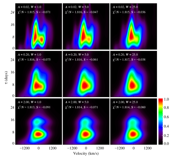
Figure 1: H$\beta$ velocity-delay maps of Mrk 142 for different values of ${\cal A}$ and ${\cal W}$ ($\alpha$ is fixed to 2000). From the left to right panels, the value of ${\cal W}$ increases by factors of 5 while the delay maps show less flexibility. From the top to bottom panels, the increasing ${\cal A}$ by factors of 10 progressively strengthens the weight of entropy in the velocity direction, and smears the sub-structure in this direction. The values of ${\cal A}$ and ${\cal W}$ in the central panel are our choice. The color bar is shown at the lower-right corner.

Since the fall of 2012, we have monitored a sample of high accretion rate AGNs, aiming at better understanding the role of accretion rates on BLRs (Du et al. 2014, hereafter Paper I; Du et al. 2015, hereafter Paper IV; Du et al. 2016a, hereafter Paper V) and the physics of accretion onto black holes (Wang et al. 2013; Wang et al. 2014b). The observations in the first three years show that super-Eddington accreting massive black holes (SEAMBHs), with $L_{\rm Bol}/L_{\rm Edd}\sim$ a few, have the following characteristics: 1) their H$\beta$ lags are significantly shorter than anticipated from the well-known BLR radius-luminosity relationship (e.g., Kaspi et al. 2000; Bentz et al. 2013), and the amount of shortening depends on the accretion rates (; ), 2) their luminosities turn out to be saturated, in accordance with predictions of the slim disk model (; ), 3) the Fe ii emission shows clear reverberation in response to the varying continuum with similar lags to those of H$\beta$ lines (Barth et al., 2013; Hu et al., 2015, hereafter Paper III). Obviously, it is necessary to investigate the details of the BLR kinematics in those extreme objects to see how they may differ from lower accretion rate AGNs.

The velocity-delay maps of the BLRs for about 11 objects have been reconstructed in the past twenty years (Ulrich & Horne, 1996; Bentz et al., 2010; Pancoast et al., 2012; Grier et al., 2013; Pancoast et al., 2014b; Grier et al., 2017). However, they are mainly AGNs with “normal” accretion rates, $L_{\rm Bol}/L_{\rm Edd}\sim 0.1$. Using the velocity-resolved time-lag analysis, we have probed the geometry and kinematics among the BLRs in 9 SEAMBH candidates monitored between 2012-2013 (hereafter SEAMBH2012) in Paper VI, identifying both disk-like and inflow/outflow signatures. In this paper, we use MEM to reconstruct velocity-delay maps for these SEAMBHs. With the high cadence and homogeneous sampling of the observations, we successfully recover velocity-delay maps of the H$\beta$ line for 6 objects and of the H$\gamma$ line for 3 objects.

The paper is organized as follows. Section 2 briefly describes the reverberation mapping (RM) observations and data reduction. Section 3 presents the methodology of MEM and the details of application to RM data. Section 4 summarizes the results of the obtained velocity-delay maps and presents discussions on individual objects. The conclusion is given in Section 5. Unless stated elsewise, time lags are given in the rest frame.

2 Observations and Data

In the first year of the campaign, 10 narrow-line Seyfert 1 galaxies (e.g., Osterbrock & Pogge 1985) were selected as SEAMBH candidates and monitored from October 2012 to June 2013 (see Table 1 in Wang et al. 2014a, hereafter Paper II). H$\beta$ time lags were detected for 9 objects. The details of telescope, spectrograph, observation and data reduction can be found in Paper I. Here we provide a brief description for completeness.

The spectroscopic monitoring was carried out using the 2.4 m telescope with the Yunnan Faint Object Spectrograph and Camera (YFOSC) at the Yunnan Observatories, from the Chinese Academy of Sciences. The spectral flux was calibrated by observing a nearby comparison star simultaneously with the target through orienting the long slit (2″.5 wide and 10′ long). The SEAMBH2012 observations had the following properties: 1) the redshifts of the targets range from 0.017 to 0.089; 2) the sampling is relatively high (interval average $\lesssim 2$ days); 3) the signal-to-noise ratios (S/N) are high (S/N$\sim$50-100); 4) the H$\beta$ lags ($\tau_{{}_{\rm H\beta}}$ $\lesssim 20$ days) are generally much shorter than the $\sim 80$ to $\sim 150$ day monitoring period; 5) the 3800-7200Å wavelength coverage allows us to recover the velocity-delay maps for different broad emission lines (e.g, H$\gamma$ and H$\beta$); 6) the spectra of the comparison stars are used to determine the line-broadening caused by instrument and seeing in each individual epoch; 7) the Fe ii emission and the host galaxy contamination have been subtracted by a fitting scheme (Paper III).

One point merits a further emphasis. The line-broadening function describes the broadening introduced by the instrument (which should not change much from epoch to epoch) and the variable seeing (which is different for each individual exposure), and widens the emission line profiles, especially for objects with relatively narrow emission lines (e.g., SEAMBHs). Crucially, because a low-resolution grism and wide slit were used during our observations (see more details in Paper VI), the line-broadening of the SEAMBH2012 observations is, on average, $\sim 500\ \rm km~{}s^{-1}$ (ranges from $\sim 350\ \rm km~{}s^{-1}$ to $\sim 800\ \rm km~{}s^{-1}$; see Figure 3 in Paper VI). The detailed line-broadening functions for different exposures can be obtained by de-convolving the spectra of the comparison stars in the slit. In Paper VI, the Richardson-Lucy deconvolution method was adopted to compensate for the line-broadening effect. In our MEM fitting, we convolve the model with the line-broadening function $\xi(\lambda)$ obtained in Paper VI:

$$L_{\rm b}(\lambda,t_{k})=L(\lambda,t_{k})\otimes\xi(\lambda)$$ (1)

to fit the observed spectra. Here $L(\lambda,t_{k})$ is the MEM modeling emission-line profile defined in the next section and $L_{\rm b}(\lambda,t_{k})$ is the broadened MEM model.

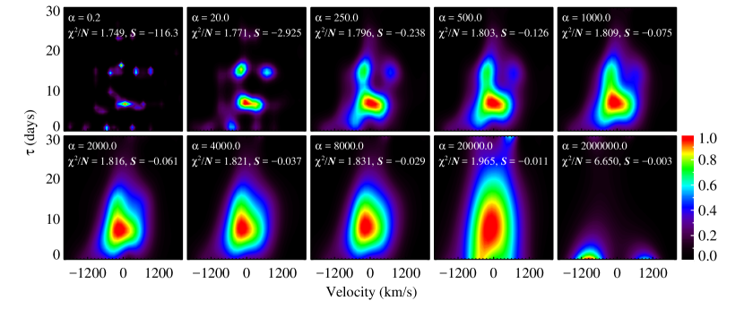
Figure 2: H$\beta$ velocity-delay maps of Mrk 142 for different values of $\alpha$ (${\cal A}$ and ${\cal W}$ are fixed to 0.2 and 5, respectively). We normalize the maps and make their peak values equal to 1. This normalization is also adopted for the velocity-delay maps hereafter. From the upper-left to the lower-right panels, we increase the value of $\alpha$. The velocity-delay map becomes smoother and $\chi^{2}/N$ increases as $\alpha$ increases. The left bottom panel ($\alpha=2000$) is our best choice for Mrk 142 because the corresponding map is reasonably smooth and the $\chi^{2}/N$ value is acceptable. The color bar is shown on the rightmost side.

3 The maximum entropy method

The MEM is a powerful technique for data fitting analysis without considering any specific model. It balances the $\chi^{2}$, which quantifies the goodness of fitting, and the entropy $S$, which represents the smoothness and simplicity of the model. The application of MEM to RM data was first developed by Horne et al. (1991). Details such as the principle and equations are discussed in Horne (1994). We generally follow the procedures of Horne (1994), but with some minor changes. For the sake of completeness, we describe the MEM and our new modifications below.

Basically, the MEM seeks a solution by minimizing

$$Q={\chi}^{2}-\alpha S,$$ (2)

where the Lagrange multiplier $\alpha\geqslant 0$ is introduced to trade off between ${\chi}^{2}$ and $S$. An undervalued $\alpha$ leads to a noisy fitting result (specifically the velocity-delay map in the following sections) and over-fitting of the data, whereas an overvalued $\alpha$ leads to an over-smoothed result and an under-fitting of the data.

In MEM, the light curves of continuum and emission line, denoted as $C(t)$ and $L(\lambda,t)$, respectively, are related by the formula

$$L(\lambda,t)=\bar{L}(\lambda)+\int_{\tau_{\rm min}}^{\tau_{\rm max}}\varPsi(\lambda,\tau)\left[C(t-\tau)-\bar{C}\right]d\tau,$$ (3)

where $\bar{C}$ and $\bar{L}(\lambda)$ are the background levels of the light curves of the continuum and emission line, respectively. They account for the non-variable components in the light curves (see the details in Horne 1994). $\varPsi(\lambda,\tau)$ is the velocity-delay map, which is a function of time lag $\tau$ and line-of-sight velocity or wavelength (i.e. $\lambda$) (e.g. Bentz et al. 2010, Pancoast et al. 2012, Grier et al. 2013). For a line at rest wavelength $\lambda_{0}$, the corresponding line-of-sight velocity is $v=c\left(\lambda-\lambda_{0}\right)/\lambda_{0}$. To apply MEM in RM data, we discretize equation (3):

$$L(\lambda_{i},t_{k})=\bar{L}(\lambda_{i})+\sum_{j}\varPsi(\lambda_{i},\tau_{j})\left[C(t_{k}-\tau_{j})-\bar{C}\right]\Delta\tau.$$ (4)

Here, $\bar{L}(\lambda_{i})$, $C(t_{k}-\tau_{j})$, and $\varPsi(\lambda_{i},\tau_{j})$ are to be determined. The primary principle underlying the MEM is to reconstruct the “simplest” $\varPsi(\lambda,\tau)$ (Skilling & Bryan 1984; Horne et al. 1991; Horne 1994) at a condition of acceptable fitting to the observed spectra.

Table 1: MEM Parameters

Object	$\alpha$	${\cal A}$	${\cal W}$	$\tau_{\rm min}$	$\tau_{\rm max}$	$\chi^{2}/N$	$N$
				(days)
Mrk 335 (H$\beta$)	800	0.5	1	-10	38	1.489	6160
Mrk 335 (H$\gamma$)	1200	0.5	1	-10	38	1.365	4224
Mrk 1044 (H$\beta$)	600	0.1	1	-10	30	2.869	1480
Mrk 1044 (H$\gamma$)	400	0.1	1	-10	30	2.034	1554
Mrk 142 (H$\beta$)	2000	0.2	5	-5	33	1.816	6000
Mrk 142 (H$\gamma$)	250	2.0	5	-2	33	1.723	4100
IRAS F12397+3333 (H$\beta$)	160	0.5	1	-10	22	1.706	1720
Mrk 486 (H$\beta$)	500	0.1	1	-5	63	1.865	2340
MCG +06-26-012 (H$\beta$)	1800	1	1	-5	58	1.518	1632

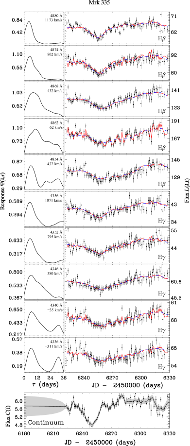
Figure 3: The best fit to the light curves at different wavelengths (in the rest frame) for Mrk 335. In each panel, the blue dashed line corresponds to the original MEM modeling light curve, and the solid red line denotes the light curve broadened by the line broadening function in each individual epoch (see $L(\lambda,t)$ and $L_{\rm b}(\lambda,t)$ in Section 2). The left panels show the corresponding 1-dimensional responses. The bottom panel shows the continuum light curve with the reconstruction of the DRW model. The selected wavelengths are labeled along the top axis of Figure 9. $C(t)$ and $L(\lambda,t)$ are in units of $10^{-15}\ {\rm erg\ s^{-1}\ cm^{-2}\ \AA^{-1}}$ and $10^{-16}\ {\rm erg\ s^{-1}\ cm^{-2}\ \AA^{-1}}$, respectively. The response $\varPsi(\lambda,t)$ is in arbitrary unit.

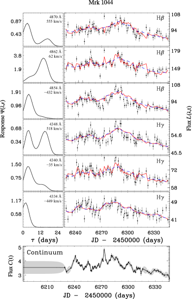
Figure 4: Same as Figure 2 but for Mrk 1044. The selected wavelengths are labeled along the top axis of Figure 10. The discarded points (see Section 4.2) are marked with black crosses.

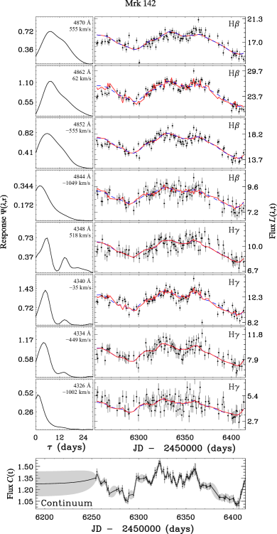
Figure 5: Same as Figure 2 but for Mrk 142. Panels are arranged as in Figure 3. The selected wavelengths are labeled along the top axis of Figure 11.

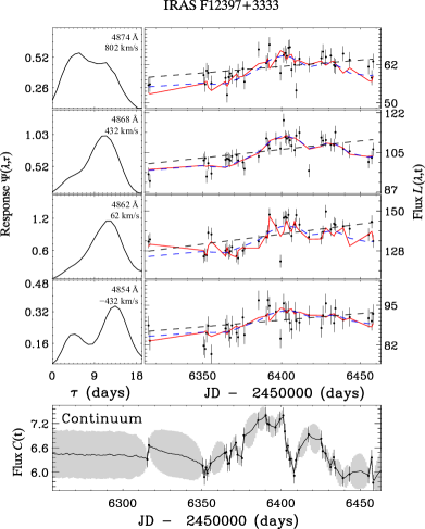
Figure 6: Same as Figure 2 but for for IRAS F12397+3333. The black dashed lines represent the trending components in the MEM model. The selected wavelengths are labeled along the top axis of Figure 12.

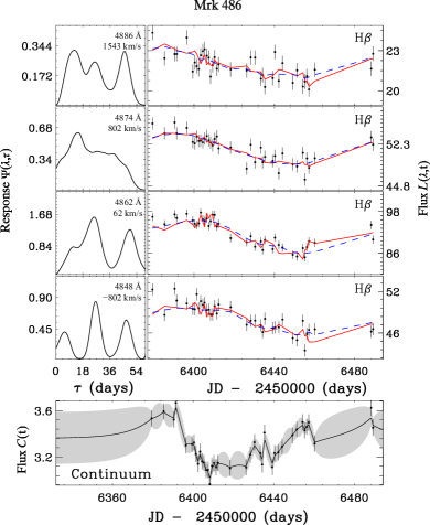
Figure 7: Same as Figure 2 but for for Mrk 486. Panels are arranged as in Figure 3. The selected wavelengths are labeled along the top axis of Figure 13.

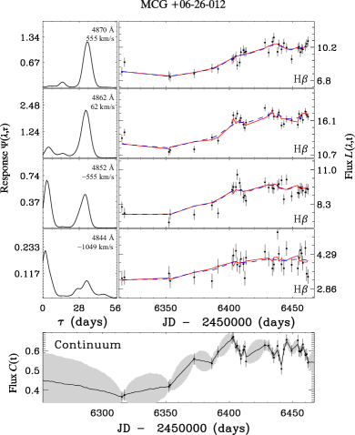
Figure 8: Same as Figure 2 but for for MCG +06-26-012. The selected wavelengths are labeled along the top axis of Figure 14.

3.1 ${\chi}^{2}$: the goodness of fitting

As in Equation (4), a velocity-delay map $\varPsi(\lambda,\tau)$ is convolved with the continuum light curve $C(t)$ to fit observations $L_{\rm obs}(\lambda_{i},t_{k})$. Here $i=1,...,N_{\lambda}$ and $k=1,...,N_{t}$ are the indexes of wavelength and epochs, respectively. The goodness of the fitting is evaluated by the usual $\chi^{2}$ as

$${\chi}^{2}=\sum_{i}\sum_{k}\left[\frac{L_{\rm obs}(\lambda_{i},t_{k})-L_{\rm b}(\lambda_{i},t_{k})}{{\sigma(\lambda_{i},t_{k})}}\right]^{2},$$ (5)

where $L_{\rm b}(\lambda_{i},t_{k})$ is the broadened MEM model defined in Equation (1) and $\sigma(\lambda_{i},t_{k})$ is the measurement error. By minimizing ${\chi}^{2}$, we obtain the closest fit to the data. However, the resulting $\varPsi(\lambda,\tau)$ is always very noisy, as previously described.

3.2 $S$: the simplicity of model

We use the definition of entropy (Horne 1994):

$$S=\sum_{m=1}^{M}\left[p_{m}-q_{m}-p_{m}\ln(p_{m}/q_{m})\right],$$ (6)

where $\{{p_{m}}\}$ are the values of parameters at $M$ grid points (e.g. of the velocity-delay map $\Psi(\lambda,\tau)$, or of the background spectrum $\bar{L}(\lambda)$) and $\{{q_{m}}\}$ are the “default values” which define the “simplest” possible model. The $\{{q_{m}}\}$ can be regarded as a function of $\{{p_{m}}\}$. The entropy is valid only for $p_{m}>0$, thus it imposes a positivity constraint on the parameters. In the MEM model, $\varPsi(\lambda,\tau)$ and $\bar{L}(\lambda)$ are described by the parameters $p_{m}$. The “default values” $q_{m}$ are set as a slightly blurred version of $p_{m}$ (Horne 1994). Following Horne (1994), we define

$$q(\lambda)=\sqrt{p(\lambda-\Delta\lambda)p(\lambda+\Delta\lambda)},$$ (7)

for the background spectrum $\bar{L}(\lambda)$. Thus for each parameter $p_{m}$ the default value $q_{m}$ is the geometric mean of its neighbors. For the velocity-delay map $\varPsi(\lambda,\tau)$, we define

$$\ln{q(\lambda,\tau)} = \dfrac{1}{1+{\cal A}}\left[\ln{\sqrt{p(\lambda-\Delta\lambda,\tau)\,p(\lambda+\Delta\lambda,\tau)}}\right.$$ (8)

$$+ \left.{\cal A}\,\ln{\sqrt{p(\lambda,\tau-\Delta\tau)\,p(\lambda,\tau+\Delta\tau)}}\right],$$

where ${\cal A}$ is a parameter that controls the relative weight of the entropies in $\tau$ and $\lambda$ directions. The choice for the value of ${\cal A}$ is discussed in Section (3.4). Minimizing the $Q$ in Equation 2 while ignoring the data is equivalent to the condition

$$\frac{\partial S}{\partial p}=-\ln(p/q),$$ (9)

so that maximizing $S$ gives $S=0$ at $p=q$. MEM draws the model toward the “simplest” model as defined by the default values $q$.

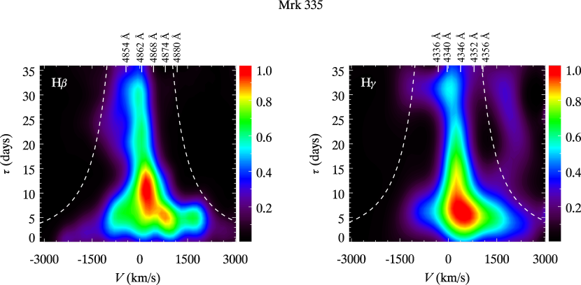
Figure 9: Velocity-delay maps of H$\beta$ and H$\gamma$ lines for Mrk 335. The dashed lines show the “virial envelope” $V^{2}\tau c/G=10^{6.87}~{}M_{\odot}$ and the labels on top axes are the corresponding rest-frame wavelengths selected in Figure 3.

3.3 Application to RM data

Detrending of light curves is used to obtain better detection of H$\beta$ lags through cross-correlation analysis, since the long-term variations possibly caused by the changes of BLR geometry and kinematics can affect the reverberation analysis (Welsh, 1999; Denney et al., 2010; Li et al., 2013). By including a detrending term, Equation (3) is rewritten as

$$L(\lambda_{i},t_{k}) = \bar{L}_{\rm trend}(\lambda_{i},t_{k})$$ (10)

$$+ \sum_{j}\varPsi(\lambda_{i},\tau_{j})\left[C(t_{k}-\tau_{j})-\bar{C}\right]\Delta\tau,$$

where $\bar{L}_{\rm trend}(\lambda_{i},t_{k})$ describes long-term trends in the line light curves. We set $\bar{C}$ as the median of continuum flux. We use a linear polynomial to represent the trending components of $\bar{L}_{\rm trend}(\lambda_{i},t_{k})$, namely, $\bar{L}_{\rm trend}(\lambda_{i},t_{k})=\bar{L}(\lambda_{i})+\left[b(\lambda_{i})-b_{0}\right]x(t_{k})$, where $x(t_{k})=2(t_{k}-\bar{t})/(t_{\rm max}-t_{\rm min})$, $b(\lambda_{i})-b_{0}$ is the linear slope to be determined and $\bar{L}(\lambda_{i})$ is the constant background. Here $\bar{t}$, $t_{\rm max}$, and $t_{\rm min}$ are the mean, maximum, and minimum times of the light curves, respectively, and $b_{0}$ is a constant. We adopt a form for $x(t_{k})$ so that it runs from -1 to +1 across the time span of the observations. In addition, We take $b(\lambda_{i})-b_{0}$ as the slope, since $b(\lambda_{i})$ is included in the entropy terms and is limited to a positive number (see Equation 6). We evaluate the slopes of the H$\beta$ line light curves of our sample, the results range between [-6.0 $\sim$ 8.2] $\times 10^{-16}\rm erg~{}s^{-1}\rm cm^{-2}\AA^{-1}$, thus we take $b_{0}=10$ ($\times 10^{-16}\rm erg~{}s^{-1}\rm cm^{-2}\AA^{-1}$), in which the slopes of the trending components $b(\lambda_{i})-b_{0}$ can range from $-10$ to $+\infty$ ($\times 10^{-16}\rm erg~{}s^{-1}\rm cm^{-2}\AA^{-1}$), and the result of our fitting can be fully optimized. We find that, except for IRAS F12397+3333, the slopes of the trending components in the other five objects are approximately zero. We thus exclude the detrending term in the fitting of these five objects to reduce the number of unknown parameters, and only take into account the detrending term in IRAS F12397+3333. For IRAS F12397+3333, the linear slope $\left[b(\lambda_{i})-b_{0}\right]/(t_{\rm max}-t_{\rm min})$ ranges between [0.007 $\sim$ 0.063]$\times 10^{-16}\rm erg~{}s^{-1}\rm cm^{-2}\AA^{-1}\rm days^{-1}$, and the average is 0.029$\times 10^{-16}\rm erg~{}s^{-1}\rm cm^{-2}\AA^{-1}\rm days^{-1}$ (see the fitting of its light curves shown in Section 4, and $t_{\rm max}-t_{\rm min}=142$ days for IRAS F12397+3333).

The total entropy of the model can be written as

$$S=\frac{S_{\bar{L}}+S_{b}+{\cal W}S_{\varPsi}}{1+{\cal W}},$$ (11)

where $S_{\bar{L}}$, $S_{b}$, and $S_{\varPsi}$ are the entropies of the background, slope, and velocity-delay map, respectively. Each term has the form shown in Equation 6. The corresponding “default value” $q$ in $S_{\bar{L}}$ and $S_{b}$ follows Equation 7, and that of $S_{\varPsi}$ follows Equation 8. The parameter ${\cal W}$ controls the weight of the entropy from the last term relative to the first two terms in the numerator of the right-hand side of Equation (11). We take $S_{\bar{L}}$ and $S_{b}$ as equal weight terms, which is different to $S_{\varPsi}$, as $\bar{L}$ and $b$ are both parts of the background spectrum and are in the same units (as described above). We changed the weight of these two terms from 0.1 to 10, to test that the general structure of the final velocity-delay maps is robust. How to select the best values for parameter ${\cal W}$ and the ${\cal A}$ (defined in Equation 8) and their influences on the velocity-delay maps are demonstrated in Horne (1994) and Grier et al. (2013). We follow their procedures and show the resulting velocity-delay maps for several potential sets of ${\cal A}$, ${\cal W}$ in Figure 1.

The continuum term $C(t_{k}-\tau_{j})$ in Equation (10) requires interpolation among the discrete measured data points. Instead of following the procedure in Horne (1994), in which the continuum light curve is treated as a component of the model, here we first interpolate the continuum light curve $C(t)$ at any given time point using a damped random walk (DRW) model (e.g., Li et al. 2013; Zu et al. 2013) and do not let it vary throughout the MEM fitting, only adjusting the velocity-delay map and the background spectra (and their trends). Thus the entropy related to the continuum light curves does not appear in Equation (11). It should be noted that fixing $C(t)$ indeed does not fully optimize $C(t)$, since the information in the $L(\lambda,t)$ light curves does not feed back into the determination of $C(t)$. However, our results should not be strongly affected because the sampling of SEAMBH2012 is high (averagely less than $\sim$2 days). In order to evaluate the influences of different continuum modeling, we compare the output maps for two approaches: one approach is adopting a simple linear interpolation of the observed continuum light curve (Appendix A) and the other is jointly modeling continuum and emission line by including the entropy of continuum into the total entropy (Appendix B). These results show that the different continuum modeling do not remarkably influence our resulting velocity-delay maps. Employing the DRW model greatly reduces the number of parameters in our model.

3.4 Control parameters $\alpha$, ${\cal A}$ and ${\cal W}$

The parameter $\alpha$ influences the final resolution of the map and plays a role in the quality of the MEM fits. Figure 2 illustrates this effect. With $\alpha$ increasing, $\chi^{2}/N$ increases but the resolution becomes lower (i.e., the fine-scale structures in the velocity-delay map disappear). However, if the value of $\alpha$ is too low, the $\chi^{2}$ term dominates the entropy term in Equation (2). As a result, the more flexible model allows MEM to overfit noise in the light curves. For each individual objects, we choose the best $\alpha$ by checking the fitting of light curves at different wavelengths and the final resolution of the map. This is similar to the procedure of Grier et al. (2013).

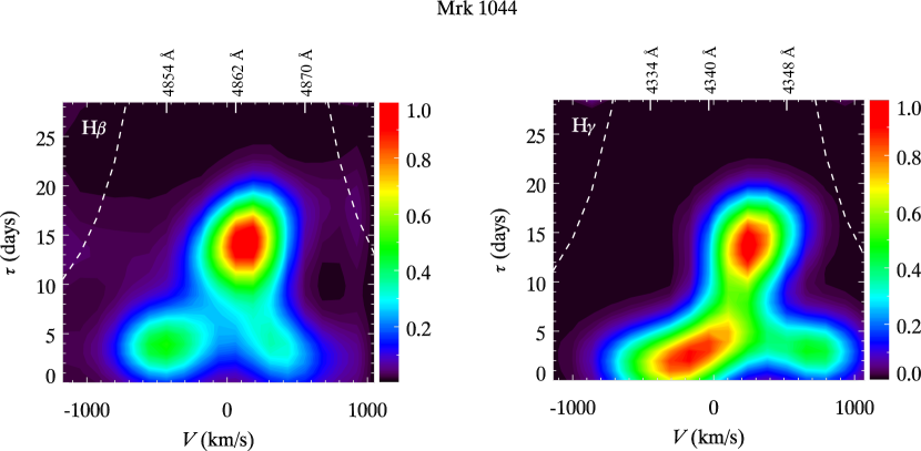
Figure 10: Velocity-delay maps of H$\beta$ and H$\gamma$ lines for Mrk 1044. The dashed lines show the “virial envelope” $V^{2}\tau c/G=10^{6.45}~{}M_{\odot}$ and the labels on top axes are the corresponding rest-frame wavelengths selected in Figure 4.

As mentioned above, ${\cal W}$ controls the weight of the entropy of the velocity-delay map relative to those of $b(\lambda)$ and $\bar{L}(\lambda)$. ${\cal A}$ controls the ratio of the entropy in velocity and $\tau$ direction. Due to the differences in the emission line widths and the observation cadences, the best values of ${\cal A}$ and ${\cal W}$ are different object-to-object. For the purpose of illustration, we plot the resulting velocity-delay maps of Mrk 142 in Figure 1, in which we alter the value of ${\cal A}$ and ${\cal W}$. Increasing ${\cal W}$ (by factors of 5 from the left to right panels) makes the map smoother and smoother. Increasing the value of ${\cal A}$ (from top to bottom panels) smears out fine structures along the velocity direction, because the weight of entropy in this direction increases. In general, the fits with different ${\cal A}$ and ${\cal W}$ are similar in the sense that the $\chi^{2}/N$ does not change significantly (much less than the influence of $\alpha$). This means that the MEM procedures are robust and relatively insensitive to ${\cal A}$ and ${\cal W}$. Here we adopt ${\cal A}$ = 0.2 and ${\cal W}$ = 5 for the H$\beta$ map of Mrk 142 as the best one, because too small or too large (${\cal A}$, ${\cal W}$) may introduce spurious small structure or make the map over-smoothed.

4 The velocity-delay maps

We apply MEM to the 9 SEAMBH candidates with significant lag measurements (8 of them are identified as SEAMBHs except for MCG +06-26-012). The fitting to the light curves of emission lines at some selected wavelengths and the corresponding one-dimensional response functions are presented in Figures 3-8. The MEM modeling light curves are relatively “noisy” after convolving with the line-broadening function, since the function varies each night. Although the individual spectra are smoother after the convolution, the light curves are noisier. For a better illustration, we plot both the original MEM modeling light curves and the broadened ones in Figure 3-8. The DRW reconstructions of the continuum light curves are also plotted in Figures 3-8. As can be seen, the variation features of light curves at different wavelengths are generally well reproduced, indicating that our MEM procedure is finding models that adequately fit light curve variations in the data of the present SEAMBH sample. The resulting velocity-delay maps are shown in Figures 9-14, and their corresponding $\alpha$, ${\cal A}$, ${\cal W}$, $\chi^{2}/N$, $N$ and the lower/upper limit $\tau_{\rm min}$/$\tau_{\rm max}$ of the delay in the MEM calculation are listed in Table 1. The selected wavelengths in Figures 3-8 are also marked along the top axis. In general, the velocity-delay maps of the 5 objects (Mrk 335, Mrk 142, Mkr 1044, Mrk 486, and MCG +06-26-012) are in good agreement with the velocity-resolved time lags. However, due to inclusion of the detrending term, the velocity-delay map of IRAS F12397+3333 shows slightly shorter time lags than the velocity-resolved time-lags from cross-correlation analysis. MCG +06-26-012 was selected as a SEAMBH candidate in our sample, but subsequent work revealed that it is a sub-Eddington object (; ).

In Figures 9-14, we also plot the “virial envelope” $V^{2}=GM_{\bullet}/c\tau$ for each object, where $G$ is the gravitational constant, $M_{\bullet}$ is black hole mass, and $c$ is the speed of light. We adopt the values of black hole mass derived in Paper IV, as listed also in the figure captions. In general, all of the observed features in the velocity-delay maps for the six objects are found within their corresponding envelopes. In principle, the response of a virialized BLR is symmetric and wider (narrower) at shorter (longer) delays and should be confined within the envelope. In contrast, the BLRs of outflow and inflow show asymmetric signatures in their velocity-delay maps. Simulated velocity-delay maps were first presented in Welsh & Horne (1991) and more recently in Figure 10 of Bentz et al. (2009) and Figure 14 of Grier et al. (2013). These provide good references for the structures found from the observations. Below we present discussions on the results for individual objects. Several outliers (one point in a spectrum of Mrk 142, and several points in five spectra for Mrk 1044 shown in Figure 4 that may influence the velocity-delay maps were traced to bad CCD pixels and then removed from the analysis.

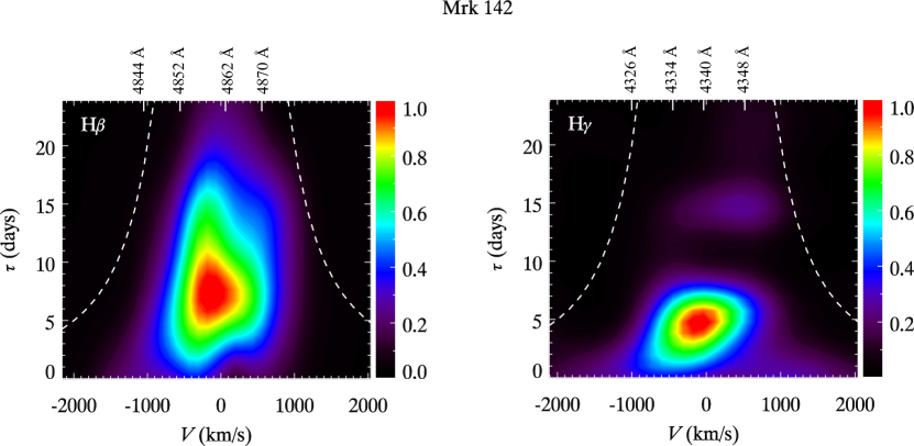
Figure 11: Velocity-delay maps of H$\beta$ and H$\gamma$ lines of Mrk 142. The dashed lines show the “virial envelope” $V^{2}\tau c/G=10^{6.59}~{}M_{\odot}$ and the labels on top axes are the corresponding rest-frame wavelengths selected in Figure 5.

4.1 Mrk 335.

We apply MEM to the data of Mrk 335 obtained in SEAMBH2012 and show its H$\beta$ and H$\gamma$ velocity-delay maps in Figure 9, with light curve fits at selected wavelengths in Figure 3. Both the H$\beta$ and H$\gamma$ maps exhibit response over a wider range of $\tau$ (0 to 30 days) in the line core than in the line wings (0 to 10 days). Equivalently, the response at small $\tau$ extends over a wider velocity range than at larger $\tau$. The red wing response is stronger than that in the blue wing, and the “red-leads-blue” asymmetric pattern is the expected signature of inflow.

Mrk 335 had been monitored spectroscopically several times in the past three decades (the campaign of 1989 - 1996 in Kassebaum et al. 1997, the campaign of 2010 - 2011 in Grier et al. 2012, and SEAMBH2012 in Paper I). Its velocity-delay map in the campaign of 2010 - 2011 (Grier et al., 2012) was provided using the two different methods (MEM in Grier et al. 2013 and dynamical modeling in Grier et al. 2017), and shows very significant signature of inflow, which is manifested as longer lags in the blue wing and shorter lags towards the red wing. A similar inflow feature was evident in the campaign of SEAMBH2012 using velocity-resolved analysis (Paper VI).

Our result is generally consistent with the kinematic signature of inflow. However, compared with the map (mainly at $\sim 15$ - $35$ days) in the campaign of 2010 - 2011 obtained by Grier et al. (2013), the response of H$\beta$ in 2012 - 2013 becomes faster ($\sim 2$ - $25$ days) and shows a potential trend of extending towards the corner of blueshift velocities and shorter lags (a trend from [$200~{}\rm km~{}s^{-1}$, 10 days] to [$-1300~{}\rm km~{}s^{-1}$, 2 days] at $\sim$50% of the maximum response level of the map). This may imply that the BLR of Mrk 335 is evolving from inflow to an inclined disk or a spherical shell. This is also supported by the lag changing from $14.3^{+0.7}_{-0.7}$ days (Grier et al. 2013) to $8.7^{+1.6}_{-1.9}$ days (Paper VI). However, the 5100 Å luminosity does not change significantly (from $43.74\pm 0.06$ to $43.69\pm 0.06$ $\rm erg~{}s^{-1}$). If we assume that the ionization parameter $U=L_{\rm ion}/4\pi R^{2}cn_{\rm H}h\nu$ is a constant (this assumption is supported by the observation of the BLR radius-luminosity relationship, see Koratkar & Gaskell 1991 and Peterson et al. 1993), where $L_{\rm ion}$ is the ionizing luminosity, $R$ is the radius of the BLR, $c$ is the speed of light, $n_{\rm H}$ is the hydrogen number density, $h$ is the Planck constant, and $\nu$ is the frequency of the ionizing photons. Clearly, this model shows that the changes in $R$ are not due to variations in $L_{\rm ion}$. Considering that two years have passed since the campaign of Grier et al. (2012), it is not unexpected that some dynamical changes began to happen in the BLR of Mrk 335. The map of H$\gamma$ is almost the same as that of H$\beta$, implying that the H$\beta$ and H$\gamma$ regions have similar kinematics and geometry.

4.2 Mrk 1044.

In Figure 10, we show the H$\beta$ and H$\gamma$ velocity-delay maps of Mrk 1044. The maps exhibit three connected features. The strongest one is at $\tau\sim 15$ days and $v\sim+200$ km s^-1. Of the two weaker ones with $\tau<5~{}$days and $v\sim\pm 500$ km s^-1, the stronger is in the blue wing, suggesting outflow.

In Paper VI, the velocity-resolved analysis divides the H$\beta$ emission line of Mrk 1044 into 4 wavelength bins and shows longer lags at smaller velocities and shorter lags at higher velocities. Such symmetric feature was interpreted as evidence of virialized motion. The H$\beta$ velocity-delay map shows similar structures. In general, the BLR of Mrk 1044 tends to be virialized. However, the overall structure of the map is accompanied by an outflow signature, with shorter response towards the blue end and longer response occurring in the red end (the average delay is 8 days for $<$ 0 $\rm km~{}s^{-1}$, and 11 days for $>$ 0 $\rm km~{}s^{-1}$). The response of the blue blob at $[-500~{}\rm km~{}s^{-1},3~{}days]$ is stronger than the red one at $[500~{}\rm km~{}s^{-1},3~{}days]$.

The H$\gamma$ map is generally similar to the H$\beta$ map, but its strongest response extends to shorter lags. It means that more H$\gamma$-emitting gas is located at smaller radius. The H$\gamma$ map shows a more definite outflow signature, although the red blob at $[700~{}\rm km~{}s^{-1},3~{}days]$ still exists. This provides an indirect support to the outflow signature found in the H$\beta$ map (considering that the H$\beta$ and H$\gamma$ lines have the same emitting mechanism).

As an AGN with extremely high accretion rate (its dimensionless accretion rate $\mathscr{\dot{M}}=\dot{M}_{\bullet}\,c^{2}/L_{\rm Edd}\sim 16.6$ where $\dot{M}_{\bullet}$ is the accretion rate and $L_{\rm Edd}$ is the Eddington luminosity; see Paper IV), the relatively stronger radiation pressure, compared with the normal AGNs, would be a likely driver of the outflow component of the BLR. Moreover, the self-shadowing effect of slim accretion disks in SEAMBHs (Wang et al., 2014b) can make the situation more complicated. The geometrically thick funnel of the inner region of a slim disk naturally leads to two dynamically distinct regions of the BLR, namely, shadowed and unshadowed regions (Wang et al., 2014b). The self-shadowing effect can be a possible reason for the very complex structure found in the H$\beta$ and H$\gamma$ map of Mrk 1044. Quantitative details of the self-shadowing effect on the BLR of Mrk 1044 need careful calculations and simulations are needed to quantitatively study the self-shadowing effects on the BLR of Mrk 1044. We defer this to a separated paper.

Figure 12: Velocity-delay maps of H$\beta$ line of IRAS F12397+3333. The dashed lines show the “virial envelope” $V^{2}\tau c/G=10^{6.79}~{}M_{\odot}$ and the labels on top axis are the corresponding rest-frame wavelengths selected in Figure 6.

4.3 Mrk 142.

In the velocity-resolved time-lag analysis of Paper VI, the longer lags in the red end and shorter lags in the blue end indicate that the BLR of Mrk 142 tends to be outflowing. Our obtained velocity-delay maps of H$\beta$ and H$\gamma$ using MEM show more details and are illustrated in Figure 11. The strongest response of H$\beta$ is located from $\sim 5$ to $\sim 11$ days at zero velocity. The velocity-resolved results from Paper VI are almost the same. It divides the H$\beta$ line into 8 bins, and the time lags at the line center are $\sim 9$ days. It should be noted that the velocity-resolved time lags are the average delays of the response in the corresponding velocity bins of the map. The response of H$\gamma$ peaks at a shorter $\sim 5$ day lag, with a weaker feature at $\sim 15$ days.

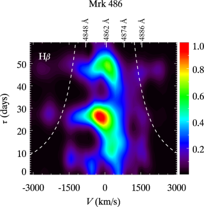
Figure 13: Velocity-delay maps of H$\beta$ line of Mrk 486. The dashed lines show the “virial envelope” $V^{2}\tau c/G=10^{7.24}~{}M_{\odot}$ and the labels on top axis are the corresponding rest-frame wavelengths selected in Figure 7.

4.4 IRAS F12397+3333.

In the velocity-resolved time-lag analysis for IRAS F12397+3333 in Paper VI, the time lags at different velocity bins are almost indistinguishable. However, we take into account the long-term trend in the emission-line light curves (see Equation (10)) and reconstruct successfully the velocity-delay map of its H$\beta$ in Figure 12. The long-term trend in our emission-line model is shown in Figure 6 as the black dashed line for each wavelength. Compared with the velocity-resolved time lags in Paper VI (which ranges from $\sim 12$ to $\sim 16$ days, except for only one bin), the velocity-delay map obtained here has slightly shorter time lags (the strongest response is located at $\sim$12 days), ascribed to the detrending of the emission line. The velocity-delay map is symmetric and consistent with the structure of an inclined disk or spherical shell (Grier et al., 2013). This is similar to the case of 3C 120 in Grier et al. (2013) or Mrk 50 in Pancoast et al. (2012).

4.5 Mrk 486 and MCG +06-26-012.

The velocity-delay maps of Mrk 486 and MCG +06-26-012 show signatures of inflow (Figure 13) and outflow (Figure 14), respectively, consistent with the velocity-resolved lags in Paper VI. The response from 35 to 55 days in the map of Mrk 486 is uncertain to some extent, because of the large gap from Julian day (hereafter JD) 2,456,460 to 2,456,488 in the H$\beta$ light curves (see Figure 7). But it should be noted that the longest response can not exceed $\sim 60$ days (the last two points in each H$\beta$ light curves have already raised up, which means that the dip is not later than $\sim$ JD 2,456,488, while the dip of the continuum is at $\sim$ JD 2,456,430). The weak feature from 0 to 7 days in the map of MCG +06-26-012 is less reliable, due to the gaps from JD 2,456,315 to 2,456,386 in the H$\beta$ light curves (see Figure 8).

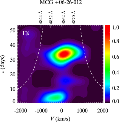
Figure 14: Velocity-delay maps of H$\beta$ line for MCG +06-26-012. The dashed lines show the “virial envelope” $V^{2}\tau c/G=10^{6.92}~{}M_{\odot}$ and the labels on top axis are the corresponding rest-frame wavelengths selected in Figure 8.

4.6 Mrk 382, Mrk 493, and IRAS 04416+1215.

We fail to reconstruct the velocity-delay maps of H$\beta$ emission lines for Mrk 382, Mrk 493, and IRAS 04416+1215, because of the relatively smaller variation amplitudes. Their maps should be obtained with future observations.

5 SUMMARY

We have reconstructed the velocity-delay maps for 6 objects in our SEAMBH2012 campaign. The BLR of Mrk 335 is consistent with an infalling dynamics, maintaining a similar structure as in the campaign of Grier et al. (2012) two years ago. Mrk 486 also shows inflow signatures in its velocity-delay map. Mrk 1044 shows a complex pattern that looks like a combination of an outflow and a symmetric component. These two components may be generated from the self-shadowing effect of slim accretion disk in SEAMBH (Wang et al., 2014b). The maps for Mrk 142 and MCG +06-26-012 also show features suggestive of an outflow, but for IRAS F12397+3333, the map is consistent with a disk-like geometry or a spherical shell. The velocity-delay maps obtained by MEM provide a basis for the model selection in dynamical modeling method in our follow-up works.

Appendix A Interpolation for continuum light curve

In the present paper, we interpolate the continuum light curves by using DRW. Whether DRW is a good description of the light curves in SEAMBHs remains to be investigated (the DRW model may not be appropriate for all AGNs, see Kasliwal et al. 2015), but this is beyond the scope of the present work. Details will be discussed in a forthcoming paper (Lu et al. 2018, in preparation). We investigate here how the output velocity-delay maps are affected if we use simple linear interpolation for the continuum light curves. We demonstrate the comparison of the reconstructed H$\beta$ maps of Mrk 335 and MCG +06-26-012 as two examples in Figure 15 and 16 for the cases of DRW-interpolated and linear-interpolated continuum light curves. The maps are denoted as $\varPsi_{\rm D}(\lambda_{i},\tau_{j})$ and $\varPsi_{\rm L}(\lambda_{i},\tau_{j})$, respectively. We adopt the same values of the MEM parameters listed in Table 1 for the reconstruction of the velocity-delay maps. The difference between the two maps can be quantified by

$$\Delta_{\rm D-L}=\frac{\sqrt{\sum_{i,j}\left[\varPsi_{\rm D}(\lambda_{i},\tau_{j})-\varPsi_{\rm L}(\lambda_{i},\tau_{j})\right]^{2}/N}}{\left(\bar{\varPsi}_{\rm max}+\bar{\varPsi}_{\rm min}\right)/2},$$ (A1)

where $\bar{\varPsi}(\lambda_{i},\tau_{j})=0.5\times[\varPsi_{\rm D}(\lambda_{i},\tau_{j})+\varPsi_{\rm L}(\lambda_{i},\tau_{j})]$ is the average map of $\varPsi_{\rm D}(\lambda_{i},\tau_{j})$ and $\varPsi_{\rm L}(\lambda_{i},\tau_{j})$, and $\bar{\varPsi}_{\rm max}$ and $\bar{\varPsi}_{\rm min}$ are the maximum and minimum of $\bar{\varPsi}(\lambda_{i},\tau_{j})$, respectively. In general, the two maps of Mrk 335 are very similar ($\Delta_{\rm D-L}$ = 0.067) and show the same signatures. The $\Delta_{\rm D-L}$ values of the other five objects (listed in Table 2) are also very small (the $\Delta_{\rm D-L}$ ranges from 0.024 to 0.083). This test shows that the continuum interpolation methods do not influence the output velocity-delay maps of the present sample very significantly.

Table 2: Differences of the map between different continuum modeling

Object	$\Delta_{\rm D-L}$	$\Delta_{\rm D-M}$
Mrk 335 (H$\beta$)	0.067	0.062
Mrk 335 (H$\gamma$)	0.071	0.077
Mrk 142 (H$\beta$)	0.024	0.055
Mrk 142 (H$\gamma$)	0.037	0.098
Mrk 1044 (H$\beta$)	0.083	0.088
Mrk 1044 (H$\gamma$)	0.063	0.096
IRAS F12397+3333 (H$\beta$)	0.029	0.060
Mrk 486 (H$\beta$)	0.053	0.051
MCG +06-26-012 (H$\beta$)	0.052	0.040

Appendix B Simultaneous MEM continuum modeling

The continuum light curve can be also modeled simultaneously with the emission-line light curves using MEM. We investigate here how the output velocity-delay maps are affected if we adopt MEM modeling to the continuum. We re-define Equation (11) as

$$S=\frac{S_{\bar{L}}+S_{b}+{\cal W}S_{\varPsi}+{{\cal W}_{C}}S_{C}}{1+{\cal W}+{{\cal W}_{C}}},$$ (B1)

where $S_{C}$ is the entropy of the continuum and ${{\cal W}_{C}}$ is a new parameter controlling the “stiffness” of $C(t)$. Following Grier et al. (2013), we model the continuum light curves by DRW first, in order to obtain better constraints on the fitting, especially in the gaps (e.g., the gaps in the light curves of Mrk 486). We then use MEM to reconstruct the continuum light curves as well as the velocity-delay maps. As two typical examples, the resulting velocity-delay maps for Mrk 335 and Mrk 486 are shown in Figures 17 and 18, respectively. We vary the ${{\cal W}_{C}}$ parameter from 0.01 to 100. The general features of the resulting maps are not affected by the changes of ${{\cal W}_{C}}$, and are consistent with the results already obtained above. The influence of the different ${{\cal W}_{C}}$ to the map of Mrk 486 is relatively stronger, because the continuum interpolation in the large gaps of its light curve becomes more flexible if adopting MEM continuum modeling. Similar to Appendix A, we define $\Delta_{\rm D-M}$ to evaluate the difference between the velocity-delay maps reconstructed for the cases of DRW-interpolated ($\varPsi_{\rm D}(\lambda_{i},\tau_{j})$) and MEM-modeled ($\varPsi_{\rm M}(\lambda_{i},\tau_{j})$) continuum light curves, and provide $\Delta_{\rm D-M}$ values (${{\cal W}_{C}}$ is fixed as 1 for $\varPsi_{\rm M}(\lambda_{i},\tau_{j})$) for the objects in Table 2. For all of the objects, $\Delta_{\rm D-M}$ values are very small (0.040$\sim$0.098). Therefore, the inclusion of continuum in the MEM reconstruction does not change the velocity-delay maps significantly.

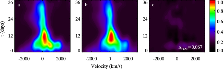
Figure 15: Comparison between the $\varPsi_{\rm D}(\lambda_{i},\tau_{j})$ and $\varPsi_{\rm L}(\lambda_{i},\tau_{j})$ of Mrk 335. Panel a shows $\varPsi_{\rm D}(\lambda_{i},\tau_{j})$, panel b shows $\varPsi_{\rm L}(\lambda_{i},\tau_{j})$, and panel c is the residual $(\varPsi_{\rm D}-\varPsi_{\rm L})$.

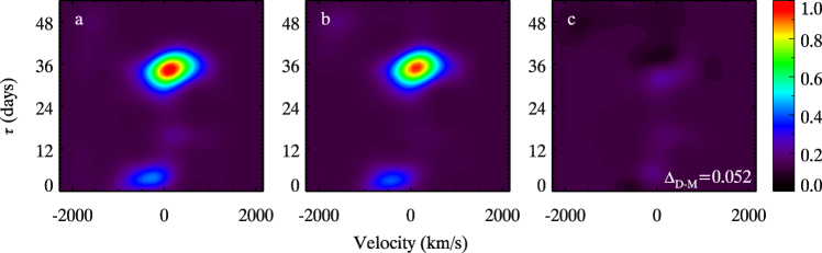
Figure 16: Comparison between the $\varPsi_{\rm D}(\lambda_{i},\tau_{j})$ and $\varPsi_{\rm L}(\lambda_{i},\tau_{j})$ of MCG +06-26-012. Panel a shows $\varPsi_{\rm D}(\lambda_{i},\tau_{j})$, panel b shows $\varPsi_{\rm L}(\lambda_{i},\tau_{j})$, and panel c is the residual $(\varPsi_{\rm D}-\varPsi_{\rm L})$.

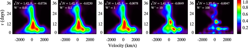
Figure 17: The velocity-delay maps of Mrk 335 reconstructed for the cases of MEM-modeled continuum light curves. From left to right, we vary $W^{\prime}$ from 0.01 to 100 (see Appendix B).

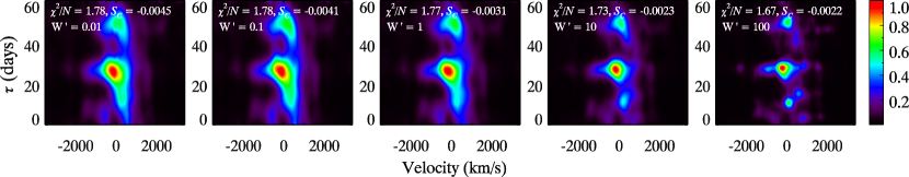
Figure 18: The velocity-delay maps of Mrk 486 reconstructed for the cases of MEM-modeled continuum light curves. From left to right, we vary $W^{\prime}$ from 0.01 to 100 (see Appendix B).

References

- Bahcall et al. (1972) Bahcall, J. N., Kozlovsky, B.-Z., & Salpeter, E. E. 1972, ApJ, 171, 467
- Barth et al. (2013) Barth, A. J., Pancoast, A., Bennert, V. N., et al. 2013, ApJ, 769, 128
- Bentz et al. (2008) Bentz, M. C., Walsh, J. L., Barth, A. J., et al. 2008, ApJ, 689, L21
- Bentz et al. (2009) Bentz, M. C., Walsh, J. L., Barth, A. J., et al. 2009, ApJ, 705, 199
- Bentz et al. (2010) Bentz, M. C., Walsh, J. L., Barth, A. J., et al. 2010, ApJ, 716, 993
- Bentz et al. (2013) Bentz, M. C., Denney, K. D., Grier, C. J., et al. 2013, ApJ, 767, 149
- Blandford & McKee (1982) Blandford, R. D., & McKee, C. F. 1982, ApJ, 255, 419
- Denney et al. (2009a) Denney, K. D., Peterson, B. M., Pogge, R. W., et al. 2009a, ApJ, 704, L80
- Denney et al. (2009b) Denney, K. D., Watson, L. C., Peterson, B. M., et al. 2009b, ApJ, 702, 1353
- Denney et al. (2010) Denney, K. D., Peterson, B. M., Pogge, R. W., et al. 2010, ApJ, 721, 715
- Du et al. (2014) Du, P., Hu, C., Lu, K.-X., et al. (SEAMBH Collaboration) 2014, ApJ, 782, 45 (Paper I)
- Du et al. (2015) Du, P., Hu, C., Lu, K.-X., et al. (SEAMBH Collaboration) 2015, ApJ, 806, 22 (Paper IV)
- Du et al. (2016a) Du, P., Lu, K.-X., Zhang, Z.-X., et al. (SEAMBH Collaboration) 2016, ApJ, 825, 126D (Paper V)
- Du et al. (2016b) Du, P., Lu, K.-X., Hu, C., et al. (SEAMBH Collaboration) 2016, ApJ, 820, 27D (Paper VI)
- Gaskell & Sparke (1986) Gaskell, C. M., & Sparke, L. S. 1986, ApJ, 305, 175cc
- Gaskell & Peterson (1987) Gaskell, C. M., & Peterson, B. M. 1987, ApJS, 65, 1
- Gaskell (1988) Gaskell, C. M., 1988, ApJ, 325, 114G
- Grier et al. (2012) Grier, C. J., Peterson, B. M., Pogge, R. W., et al. 2012, ApJ, 755, 60
- Grier et al. (2013) Grier, C. J., Peterson, B. M., Horne, K., et al. 2013, ApJ, 764, 47
- Grier et al. (2017) Grier, C. J., Pancoast, A., Barth, A. J., et al. 2017, arXiv:1705.02346
- Kaspi et al. (2000) Kaspi, S., Smith, P. S., Netzer, H., et al. 2000, ApJ, 533, 631
- Kasliwal et al. (2015) Kasliwal, V. P., Vogeley, M. S., & Richards, G. T. 2015, MNRAS, 451, 4328
- Kassebaum et al. (1997) Kassebarm, T. M., Peterson, B. M., Wanders, I., et al. 1997, ApJ, 475, 106
- Koratkar & Gaskell (1991) Koratkar, A. P., & Gaskell, C. M. 1991, ApJS, 75, 719
- Li et al. (2013) Li, Y.-R., Wang, J.-M., Ho, L. C., Du, P., & Bai, J.-M. 2013, ApJ, 779, 110
- Horne et al. (1991) Horne, K., Welsh, W. F., & Peterson, B.M. 1991, ApJL, 367, 5
- Horne (1994) Horne, K. 1994, in ASP Conf. Ser. 69, Reverberation Mapping of the Broad-line Region in Active Galactic Nuclei, ed. P.M. Gondhalekar, K. Horne, & B.M. Peterson (San Francisco, CA: ASP), 23
- Hu et al. (2015) Hu, C., Du, P., Lu, K.-X., et al. (SEAMBH Collaboration) 2015, ApJ, 804, 138 (Paper III)
- Osterbrock & Pogge (1985) Osterbrock, D. E., & Pogge, R. W. 1985, ApJ, 297, 166
- Osterbrock (1989) Osterbrock, D. E. 1989, Astrophysics of gaseous nebulae and active galactic nuclei (Mill Valley, CA: University Science Books)
- Pancoast et al. (2011) Pancoast, A., Brewer, B.J., & Treu, T. 2011, ApJ, 670, 105
- Pancoast et al. (2012) Pancoast, A., Brewer, B.J., Treu, T., et al. 2012, ApJ, 730, 139
- Pancoast et al. (2014a) Pancoast, A., Brewer, B.J., & Treu, T. 2014, MNRAS, 445, 3055
- Pancoast et al. (2014b) Pancoast, A., Brewer, B.J., & Treu, T. 2014, MNRAS, 445, 3073
- Peterson et al. (1993) Peterson, B. M., Ali, B., Horne, K., et al. 1993, PASP, 105, 247
- Skilling & Bryan (1984) Skilling, J., & Bryan, R. K. 1984, MNRAS, 211, 111
- Ulrich & Horne (1996) Ulrich, M.-H., & Horne, K. 1996, MNRAS, 283, 748
- Wang et al. (2013) Wang, J.-M., Du, P., Valls-Gabaud, D., Hu, C., & Netzer, H. 2013, Phys. Rev. Lett., 110, 081301
- Wang et al. (2014a) Wang, J.-M., Du, P., Hu, C., et al. (SEAMBH Collaboration) 2014a, ApJ, 793, 108 (Paper II)
- Wang et al. (2014b) Wang, J.-M., Qiu, J., Du, P., & Ho, L. C. 2014b, ApJ, 797, 65
- Welsh & Horne (1991) Welsh, W. F., & Horne, K. 1991, ApJ, 379, 586
- Welsh (1999) Welsh, W. F. 1999, PASP, 111, 1347
- Zu et al. (2013) Zu, Y., Kochanek, C. S., Kozlowski, S., & Udalski, A. 2013, ApJ, 765, 106