A diagonal PRP-type projection method for convex constrained nonlinear monotone equations

Abstract

Iterative methods for nonlinear monotone equations do not require the differentiability assumption on the residual function. This special property of the methods makes them suitable for solving large-scale nonsmooth monotone equations. In this work, we present a diagonal Polak-Ribi$\grave{e}$re-Polyk (PRP) conjugate gradient-type method for solving large-scale nonlinear monotone equations with convex constraints. The search direction is a combine form of a multivariate (diagonal) spectral method and a modified PRP conjugate gradient method. Proper safeguards are devised to ensure positive definiteness of the diagonal matrix associated with the search direction. Based on Lipschitz continuity and monotonicity assumptions the method is shown to be globally convergent. Numerical results are presented by means of comparative experiments with recently proposed multivariate spectral conjugate gradient-type method.

Keywords: Nonlinear monotone equations, diagonal spectral gradient method, PRP conjugate gradient method
Mathematics Subject Classification: 65K05, 90C06, 90C56.

1.   Introduction

In this paper, we address the following constrained monotone equations

$$F(x^{*})=0,~{}~{}x^{*}\in\Omega,$$ (1)

where $\textbf{F}:\Omega\to\mathbb{R}^{n}$ is continuous and monotone function, on a non-empty closed convex set $\Omega\in\mathbb{R}^{n}$. The monotonicity of $F$ here means $\langle\,F(x)-F(y),x-y\rangle\geq 0,~{}~{}\forall x,y\in\Omega$

The system of monotone equations has various applications [15, 8, 40, 5], e.g the $\ell_{1}$-norm problem arising from compressing sensing [34, 20, 17], generalized proximal algorithm with Bregman distances [11], variational inequalities problems [27, 6], and optimal power flow equations [33, 7] among others.

At the case where $\Omega=\mathbb{R}^{n}$, Solodov and Svaiter [28] combined Newton’s method and projection strategy and proposed a global convergent inexact Newton method for system of monotone equations without the differentiability assumption. Wang et. al [31] extended the work by Solodov and Svaiter to solve convex constrained monotone equations. Since then many methods for solving system of nonlinear monotone equations have been proposed (see, e.g. [37, 30, 12, 29, 21, 32, 24, 25, 10, 18, 38, 39, 23, 42, 13, 16, 2, 35, 26, 1], among others). Specifically, Ma and Wang [22] proposed a modified projection method for solving a system of monotone equations with convex constraints. Though the projection methods for convex constrained monotone equations proposed in [31] and [22] have a very good numerical performance, they are not suitable for solving large-scale monotone equations because they require matrix storage.

By taking the advantage of the good performance of the multivariate (diagonal) spectral gradient method by Han et. al. [9], Yu et. al. [36] proposed a multivariate spectral gradient projection method for nonlinear monotone equations with convex constraints. Recently, Liu and Li [19] proposed a multivariate spectral conjugate gradient-type projection algorithm for constrained nonlinear monotone equations by combining the multivariate spectral gradient method and the Dai-Yuan (DY) conjugate gradient method.

Motivated by the development of the diagonal spectral gradient projection approach for constrained nonlinear monotone equations, in this paper, we extend the sufficient descent modified Polak-Ribi$\grave{e}$re-Polyk (PRP) nonlinear conjugate gradient method proposed by Dong et. al.[4] to solve nonlinear monotone equations with convex constraints. We show that the proposed method has some attractive properties, for example, it is a derivative-free and matrix-free method. Hence, it is suitable for solving non-smooth and large-scale problems. Under the monotonicity and Lipschitz continuity assumptions on $F$, we show that the proposed algorithm is globally convergent.

The outstanding part of this paper is organized as follows. In Section 2 we present the algorithm of the proposed method. In Section 3 we establish the global convergence of the proposed method. In section 4 we present the numerical experiments, and conclusions in Section 5. Unless otherwise stated, throughout this paper $\|.\|$ stands for the Euclidean norm of vectors and the induced $2$-norm of matrices, $\langle\,.~{},~{}.\rangle$ is the inner product of vectors in $\mathbb{R}^{n}$.

2.   A diagonal PRP-type projection method

We begin this section by describing the unconstrained convex optimization problem

$$\min_{x\in\mathbb{R}^{n}}f(x),$$ (2)

where $f:\mathbb{R}^{n}\to\mathbb{R}$ is a continuously differentiable function with gradient $g(x_{k})=\nabla f(x_{k})$. The descent modified Polak-Ribi$\grave{e}$re-Polyk (PRP) conjugate gradient method proposed by Dong et. al. [4] generates a sequence $\{x_{k}\}$ that satisfies

$$x_{k+1}=x_{k}+\alpha_{k}d_{k},~{}~{}~{}k=0,1,...,$$ (3)

where where $\alpha_{k}>0$ is a steplength, $d_{k}$ is a search direction generated by

$$d_{k}=\begin{cases}-g(x_{0}),~{}~{}~{}\text{if }k=0\\[10.0pt] -g(x_{k})+\beta_{k}d_{k-1},~{}~{}~{}\text{if }k\geq 1,\end{cases}$$ (4)

where $\beta_{k}$ is defined by

$$\beta_{k}=\max\biggl{\{}0,\frac{\langle g(x_{k}),y_{k-1}\rangle}{\|g(x_{k-1})\|^{2}}-t\frac{\langle g(x_{k}),d_{k-1}\rangle}{\|g(x_{k-1})\|^{4}}\biggl{(}\frac{\langle g(x_{k}),y_{k-1}\rangle}{\|g(x_{k})\|}\biggr{)}^{2}\biggr{\}},$$ (5)

where $y_{k-1}=g(x_{k})-g(x_{k-1}),~{}~{}t>\frac{1}{4}$ is a given positive constant.

Based on the formulae (3)-(5), we introduce our method for solving (1). Inspired by (4) we redefine $d_{k}$ as

$$d_{k}=\begin{cases}-D_{0}F(x_{0}),~{}~{}~{}\text{if }k=0\\[10.0pt] -D_{k}F(x_{k})+\beta_{k}d_{k-1},~{}~{}~{}\text{if }k\geq 1,\end{cases}$$ (6)

where $D_{0}=I_{n},~{}D_{k}$ is a positive definite diagonal matrix given by

$$D_{k}=\text{diag}\biggl{(}\frac{1}{\lambda_{k}^{1}},\frac{1}{\lambda_{k}^{2}},...,\frac{1}{\lambda_{k}^{n}}\biggr{)},$$ (7)

$$\lambda_{k}^{i}=\begin{cases}{y_{k-1}^{i}\over s_{k-1}^{i}},&\text{ if }{y_{k-1}^{i}\over s_{k-1}^{i}}>0\\[15.0pt] \delta,&\text{ if }{y_{k-1}^{i}\over s_{k-1}^{i}}\leq 0\text{ or }s_{k-1}^{i}=0.\end{cases}$$ (8)

where $y_{k-1}=F(x_{k})-F(x_{k-1}),~{}s_{k-1}=x_{k}-x_{k-1},\text{ and }\delta>0$ is chosen as a safeguard that ensures all the entries of the diagonal matrix are positive. $\beta_{k}$ is defined as

$$\beta_{k}=\max\biggl{\{}0,\frac{\langle F(x_{k}),y_{k-1}\rangle}{\|F(x_{k-1})\|^{2}}-t\frac{\langle F(x_{k}),d_{k-1}\rangle}{\|F(x_{k-1})\|^{4}}\biggl{(}\frac{\langle F(x_{k}),y_{k-1}\rangle}{\|F(x_{k})\|}\biggr{)}^{2}\biggr{\}}.$$ (9)

Observe that, if the diagonal components the matrix $D_{k}$ are negative, a non-negative scalar $\delta$ is used as a safeguard. The common choice of $\delta$ in most of the previous works [9, 19, 36] is

$$\delta=\frac{\langle s_{k-1},~{}y_{k-1}\rangle}{\langle s_{k-1},~{}s_{k-1}\rangle}.$$ (10)

However, we feel that there may be better choices for replacing $\lambda_{k}^{i}$ when it is negative. In what follows, we present a simple approach for choosing the value of the scalar $\delta$.

The scalar $\lambda_{k}^{i}$ is non-positive if and only if

$$s_{k-1}^{i}<0\text{ and }y_{k-1}^{i}\geq 0,$$

or

$$s_{k-1}^{i}>0\text{ and }y_{k-1}^{i}\leq 0.$$

In the first case, it is better to choose a non-positive scalar that carries some information about the current value of $y_{k-1}$. Similarly, in the second case, it is better to choose a non-negative scalar that carries some information about the current value of $y_{k-1}$. We now present our simple safeguard for choosing the replacement of $\lambda_{k}^{i}$ in case it is negative. We consider the following two cases, in which $\theta\in(0,1)$ is a shrinking factor, and $\epsilon>0$ is a tolerance for ensuring strictly positive values, $i=1,2,..,n.$

CASE I: Assume that $s_{k-1}^{i}>0$.

$$\quad\text{If }y_{k-1}^{i}\leq 0\implies F(x_{k})^{i}-F(x_{k-1})^{i}\leq 0\implies F(x_{k})^{i}\leq F(x_{k-1})^{i}.$$

In this case, we redefine

$$y_{k-1}^{i}=\theta\max\bigl{\{}\max\bigl{\{}|F(x_{k})^{i}|,|F(x_{k-1})^{i}|\bigr{\}},\epsilon\bigr{\}},$$ (11)

so that $\lambda_{k}^{i}={y_{k-1}^{i}\over s_{k-1}^{i}}>0.$

CASE II: Assume that $s_{k-1}^{i}<0.$

$$\quad\text{If }y_{k-1}^{i}\geq 0\implies F(x_{k})^{i}-F(x_{k-1})^{i}\geq 0\implies F(x_{k})^{i}\geq F(x_{k-1})^{i}.$$

In this case, we redefine

$$y_{k-1}^{i}=-\theta\max\bigl{\{}\max\bigl{\{}|F(x_{k})^{i}|,|F(x_{k-1})^{i}|\bigr{\}},\epsilon\bigr{\}},$$ (12)

so that $\lambda_{k}^{i}={y_{k-1}^{i}\over s_{k-1}^{i}}>0.$

Next we state our algorithm. We used the projection operator

$$P_{\Omega}[x]:=\text{arg min}_{y\in\Omega}\{\|y-x\|\},$$

that denotes the projection of $x$ on the closed convex set $\Omega$, to ensure the new point generated by our algorithm is a member of the domain of definition. It is not difficult to notice that if $x\in\Omega$, the value of $P_{\Omega}[x]$ is equal to $x$. In addition, $P_{\Omega}[x]$ is nonexpansive, that is

$$\|P_{\Omega}[x]-P_{\Omega}[y]\|\leq\|x-y\|,~{}~{}~{}\forall x,y\in\mathbb{R}^{n}.$$ (13)

1 input :  Given $x_{0}\in\mathbb{R}^{n},~{}\Omega\in\mathbb{R}^{n},~{}\rho,~{}\sigma,~{}\theta,\in(0,1)$,  $0<\ell\leq 1\leq u$ and $\epsilon,~{}\mu,~{}tol>0$.

2 Set $k=0,~{}D_{k}=I$, where $I$ is an $n\times n$ identity matrix;

3 Compute $\|F(x_{k})\|$;

4 while $\|F(x_{k})\|>tol$  do

      5 Compute $d_{k}=-D_{k}F(x_{k})$;

      6 Initialize $m=0$;

      7 while $\langle\,F(x_{k}+\beta\rho^{m}d_{k}),~{}d_{k}\rangle>-\sigma\beta\rho^{m}\|F(x_{k}+\beta\rho^{m}d_{k})\|\|d_{k}\|^{2}$  do

            8 $m=m+1$;

            9 $\alpha=\beta\rho^{m}$;

            

       end while

      10Set $\alpha_{k}=\alpha$;

      11 Compute $z_{k}=x_{k}+\alpha_{k}d_{k}$;

      

      12if $z_{k}\in\Omega\text{ and }F(z_{k})\leq tol$  then

            $x_{k+1}=z_{k}$

       end if

      13$x_{k+1}=P_{\Omega}[x_{k}-\xi_{k}F(x_{k})],$ where $\xi_{k}=\frac{\langle\,x_{k}-z_{k},~{}F(z_{k})\rangle}{\|F(z_{k})\|^{2}}$;

      14 Compute $s_{k}=x_{k+1}-x_{k},~{}~{}y_{k}=F(x_{k+1})-F(x_{k})$;

      15 Compute

$$\lambda_{k+1}^{i}=\begin{cases}\max\bigl{\{}\min\bigl{\{}\frac{y_{k}^{i}}{s_{k}^{i}},~{}~{}u\bigr{\}},~{}~{}\ell\big{\}},&\text{ if }s_{k}^{i}\neq 0\\ 1,&\text{ if }s_{k}^{i}=0.\end{cases}$$ (14)

where $y_{k}^{i}$ is safeguarded for possible different signs with $s_{k}^{i},$ using Equations (11) and (12);

      16 Compute $D_{k+1}$ by (7) and $\beta_{k+1}$ by (9);

      17 Compute

$$d_{k+1}=\begin{cases}-D_{k+1}F(x_{k+1}),&\text{ if }|\langle F(x_{k+1}),y_{k}\rangle|\|d_{k}\|\geq\mu\|F(x_{k+1})\|,\\[10.0pt] -D_{k+1}F(x_{k+1})+\beta_{k+1}d_{k},&\text{ if }|\langle F(x_{k+1}),y_{k}\rangle|\|d_{k}\|<\mu\|F(x_{k+1})\|.\end{cases}$$ (15)

      18Set $k=k+1$.

end while

Algorithm 1 Diagonal PRP Projection Method (DPPM)

Remark 2.1

Since the matrix $D_{k}$ is diagonal, the product at line 1 of Algorithm 1 is simply the product between the elements of $D_{k}$ and the corresponding components of $F(x_{k})$, computed in $\emph{O}(n)$ operations. Also by definition of $D_{k}$ at line 1, $D_{k}$ is positive definite.

Remark 2.2

The sequence $\{\lambda_{k+1}^{i}\}$ at line 1 is uniformly bounded for each $i\text{ and }k$. It is clear that

$$\ell\leq\lambda_{k+1}^{i}\leq u~{}~{}\forall i,~{}~{}\forall k.$$

Remark 2.3

The update rule for the search direction at line 1, is given specifically to ensure global convergence of the Algorithm DPPM.

Now, we show a nice property of the search direction defined in (15), which is quite significance in the construction of our algorithm. The proof is similar to [4] [Lemma 2.1] but with different definition for the right-hand term of the search direction.

Lemma 2.4

Let $\{d_{k}\}$ be the sequence generated by (15), $\beta_{k}$ is given by (9). Then there exists a constant $c>0$ such that

$$\bigl{\langle}\,F(x_{k}),~{}d_{k}\bigr{\rangle}\leq-c\bigl{\|}F(x_{k})\bigr{\|}^{2},~{}~{}\forall k\geq 0.$$ (16)

Proof  For $k=0$, we have

$$\begin{split}\langle F(x_{0}),~{}d_{0}\rangle&=\langle F(x_{0}),~{}-D_{0}F(x_{0})\rangle\\ &=\langle F(x_{0}),~{}-F(x_{0})\rangle\quad\text{since }D_{0}=I\\ &=-\|F(x_{0})\|^{2}.\end{split}$$

For $k\geq 1,$ we consider two cases:

Case (i) If $\frac{\langle F(x_{k}),y_{k-1}\rangle}{\|F(x_{k-1})\|^{2}}\leq t\frac{\langle F(x_{k}),d_{k-1}\rangle}{\|F(x_{k-1})\|^{4}}\biggl{(}\frac{\langle F(x_{k}),y_{k-1}\rangle}{\|F(x_{k})\|}\biggr{)}^{2}$, then $\beta_{k}=0$. Therefore,

$$\begin{split}\langle F(x_{k}),~{}d_{k}\rangle&=\langle F(x_{k}),~{}-D_{k}F(x_{k})\rangle\\ &=\biggl{\langle}F(x_{k}),~{}\text{diag}\biggl{(}\frac{-1}{\lambda_{k}^{1}},\frac{-1}{\lambda_{k}^{2}},...,\frac{-1}{\lambda_{k}^{n}}\biggr{)}F(x_{k})\biggr{\rangle}\\ &\leq\biggl{\langle}F(x_{k}),~{}\text{diag}\biggl{(}\frac{-1}{u},\frac{-1}{u},...,\frac{-1}{u}\biggr{)}F(x_{k})\biggr{\rangle}\\ &=-\frac{1}{u}\langle F(x_{k}),~{}F(x_{k})\rangle\\ &=-c\|F(x_{0})\|^{2},\quad 0<c=\frac{1}{u},\end{split}$$

where the first inequality follows from the boundedness of $\frac{-1}{\lambda_{k}^{i}},~{}~{}~{}i=1,2,\ldots n.$

Case (ii) If $\frac{\langle F(x_{k}),y_{k-1}\rangle}{\|F(x_{k-1})\|^{2}}>t\frac{\langle F(x_{k}),d_{k-1}\rangle}{\|F(x_{k-1})\|^{4}}\biggl{(}\frac{\langle F(x_{k}),y_{k-1}\rangle}{\|F(x_{k})\|}\biggr{)}^{2}$, then we have

$$\begin{split}\langle F(x_{k}),~{}d_{k}\rangle&=\langle F(x_{k}),~{}-D_{k}F(x_{k})+\beta_{k}d_{k-1}\rangle\\ &=\biggl{\langle}F(x_{k}),~{}\text{diag}\biggl{(}\frac{-1}{\lambda_{k}^{1}},\frac{-1}{\lambda_{k}^{2}},...,\frac{-1}{\lambda_{k}^{n}}\biggr{)}F(x_{k})\biggr{\rangle}\\ &\quad\quad\quad+\biggl{\langle}F(x_{k}),~{}\frac{\langle F(x_{k}),y_{k-1}\rangle}{\|F(x_{k-1})\|^{2}}d_{k-1}-t\frac{\langle F(x_{k}),d_{k-1}\rangle}{\|F(x_{k-1})\|^{4}}\biggl{(}\frac{\langle F(x_{k}),y_{k-1}\rangle}{\|F(x_{k})\|}\biggr{)}^{2}d_{k-1}\biggr{\rangle}\\ &\leq\biggl{\langle}F(x_{k}),~{}\text{diag}\biggl{(}\frac{-1}{u},\frac{-1}{u},...,\frac{-1}{u}\biggr{)}F(x_{k})\biggr{\rangle}\\ &\quad\quad\quad+\biggl{\langle}F(x_{k}),~{}\frac{\langle F(x_{k}),y_{k-1}\rangle}{\|F(x_{k-1})\|^{2}}d_{k-1}\biggr{\rangle}+\biggl{\langle}F(x_{k}),~{}-t\frac{\langle F(x_{k}),d_{k-1}\rangle}{\|F(x_{k-1})\|^{4}}\biggl{(}\frac{\langle F(x_{k}),y_{k-1}\rangle}{\|F(x_{k})\|}\biggr{)}^{2}d_{k-1}\biggr{\rangle}\end{split}$$

$$\begin{split}&\quad\quad\quad\quad\quad=-\biggl{(}\frac{1}{u}-\frac{1}{4t}\biggr{)}\biggl{\langle}F(x_{k}),~{}F(x_{k})\biggr{\rangle}+\biggl{[}-\frac{\bigl{\langle}F(x_{k}),~{}F(x_{k})\bigr{\rangle}}{4t}+\frac{\langle F(x_{k}),y_{k-1}\rangle}{\|F(x_{k-1})\|^{2}}\biggl{\langle}F(x_{k}),~{}d_{k-1}\biggr{\rangle}\\ &\quad\quad\quad\quad\quad\quad\quad\quad-t\frac{\langle F(x_{k}),d_{k-1}\rangle^{2}}{\|F(x_{k-1})\|^{4}}\biggl{(}\frac{\langle F(x_{k}),y_{k-1}\rangle}{\|F(x_{k})\|}\biggr{)}^{2}\biggr{]}.\end{split}$$ (17)

By applying the inequality $2ab\leq a^{2}+b^{2}$ to the second term of (17) with $a=\frac{1}{2\sqrt{t}}\|F(x_{k})\|$ and $b=\sqrt{t}\frac{\langle F(x_{k}),d_{k-1}\rangle}{\|F(x_{k-1})\|^{2}}~{}.~{}\frac{\langle F(x_{k}),y_{k-1}\rangle}{\|F(x_{k})\|},$ we have

$$\bigl{\langle}\,F(x_{k}),~{}d_{k}\bigr{\rangle}\leq-c\bigl{\|}F(x_{k})\bigr{\|}^{2},$$

where $0<c=\frac{1}{u}-\frac{1}{4t}\implies t>\frac{u}{4},\quad u\geq 1$.   

3.   Convergence Analysis

We now turn to analyze the global convergence of Algorithm 1 (DPPM). First we state the following standard assumptions:

Assumption 3.1

The function $F:\mathbb{R}^{n}\to\mathbb{R}^{n}$ is continuously differentiable and monotone.

Assumption 3.2

The function $F$ is Lipschitz continuous on $\Omega$, i.e., there exists a constant $L>0$ such that

$$\|F(x)-F(y)\|\leq L\|x-y\|,~{}~{}~{}\forall x,y\in\Omega.$$ (18)

Assumption 3.3

The solution set of (1) denoted by $\Phi$ is convex and nonempty.

In addition, we also assume that $F(x)\neq 0,\quad\forall x\neq x^{*}$, otherwise the solution of Equation (1) has been obtained.

Lemma 3.4

The Algorithm 1 (DPPM) is well defined.

Proof  Suppose that there exists $k_{0}\geq 0,$ such that

$$\langle\,F(x_{k_{0}}+\beta\rho^{m}d_{k_{0}}),~{}d_{k_{0}}\rangle>-\sigma\beta\rho^{m}\|F(x_{k_{0}}+\beta\rho^{m}d_{k_{0}})\|\|d_{k_{0}}\|^{2},~{}~{}\forall m\geq 0.$$

By continuity of $F$, allowing $m\to+\infty$, we have

$$\langle\,F(x_{k_{0}}),~{}d_{k_{0}}\rangle\geq 0,$$

which contradits the conclusion of Lemma 2.4.   

The proof of the following Lemma is similar to that of [20].

Lemma 3.5

Let $\{x_{k}\},\text{ and }\{z_{k}\}$ be the sequences generated by Algorithm 1. Then $\{x_{k}\},\text{ and }\{z_{k}\}$ are bounded. In addition,

$$\lim_{k\to+\infty}\|x_{k}-z_{k}\|=0,\text{ more specifically }\lim_{k\to+\infty}\alpha_{k}\|d_{k}\|=0.$$

and

$$\lim_{k\to+\infty}\|x_{k+1}-x_{k}\|=0.\$$

Lemma 3.6

Let $\{x_{k}\},\text{ and }\{d_{k}\}$ be the sequences generated by Algorithm 1. If there exists a constant $\varepsilon>0$ such that $\|F(x_{k-1})\|\geq\varepsilon,\quad k\geq 1,$ then there exists a constant $\hat{c}>0$ such that

$$\|d_{k}\|\leq\hat{c}\|F(x_{k})\|\quad\forall k\in\mathbb{N}\cup\{0\}.$$ (19)

Proof  By the definition of $d_{k}$ in line 1 of Algorithm 1. If $|\langle F(x_{k}),y_{k-1}\rangle|\|d_{k-1}\|\geq\mu\|F(x_{k})\|,$ we have

$$\|d_{k}\| =\|D_{k}F(x_{k})\|$$

$$\leq\|D_{k}\|\|F(x_{k})\|$$

$$\leq\frac{\sqrt{n}}{\ell}\|F(x_{k})\|$$

$$=\hat{c}\|F(x_{k})\|,$$

with $0<\hat{c}=\frac{\sqrt{n}}{\ell},$ where the first inequality follows from the induced matrix norm property, and the second inequality follows from the boundedness of the components of $D_{k}$.

On the other hand, if $|\langle F(x_{k}),y_{k-1}\rangle|\|d_{k-1}\|<\mu\|F(x_{k})\|,$ we have

$$\|d_{k}\| =\|-D_{k}F(x_{k})+\beta_{k}d_{k-1}\|$$

$$\leq\|D_{k}F(x_{k})\|+|\beta_{k}\|\|d_{k-1}\|$$

$$\leq\|D_{k}\|\|F(x_{k})\|+\frac{|\langle F(x_{k}),y_{k-1}\rangle|}{\|F(x_{k-1})\|^{2}}\|d_{k-1}\|$$

$$\quad\quad+\frac{|\langle F(x_{k}),d_{k-1}\rangle|}{\|F(x_{k-1})\|^{4}}~{}.~{}\frac{\langle F(x_{k}),y_{k-1}\rangle^{2}}{\|F(x_{k})\|^{2}}\|d_{k-1}\|$$

$$\leq\frac{\sqrt{n}}{\ell}\|F(x_{k})\|+\frac{\mu\|F(x_{k})\|}{\|F(x_{k-1})\|^{2}}+t\frac{\mu^{2}\|F(x_{k})\|}{\|F(x_{k-1})\|^{4}}$$

$$\leq\biggl{(}\frac{\sqrt{n}}{\ell}+\frac{\mu}{\varepsilon^{2}}+t\frac{\mu^{2}}{\varepsilon^{4}}\biggr{)}\|F(x_{k})\|$$

$$=\hat{c}\|F(x_{k})\|,$$

with $0<\hat{c}=\frac{\sqrt{n}}{\ell}+\frac{\mu}{\varepsilon^{2}}+t\frac{\mu^{2}}{\varepsilon^{4}},$ where the second inequality is obtained from the induced matrix norm property, the third inequality follows directly from the boundedness of $D_{k}$, the Cauchy Schwartz inequality and the fact that $|\langle F(x_{k}),y_{k-1}\rangle|\|d_{k-1}\|<\mu\|F(x_{k})\|.$ And the proof is complete.   

Now, we are ready to establish the global convergence of Algorithm 1.

Theorem 3.7

Let $\{x_{k}\},\text{ and }\{z_{k}\}$ be the sequences generated by Algorithm 1. Then

$$\liminf_{k\to\infty}\|F(x_{k})\|=0.$$ (20)

Furthermore, the sequence $\{x_{k}\}$ converges to $\tilde{x}\in\Omega$ such that $F(\tilde{x})=0$.

Proof  If $\displaystyle\liminf_{k\to\infty}\|d_{k}\|=0,$ we have $\displaystyle\liminf_{k\to\infty}\|F(x_{k})\|=0.$

Suppose $\displaystyle\liminf_{k\to\infty}\|d_{k}\|>0,$ we have $\displaystyle\liminf_{k\to\infty}\|F(x_{k})\|>0.$
Using the line search in line (1) of Algorithm 1,

$$-F(x_{k}+\beta\rho^{m_{k-1}}d_{k})^{T}d_{k}<\sigma\beta\rho^{m_{k-1}}\|F(x_{k}+\beta\rho^{m_{k-1}}d_{k}\|\|d_{k}\|^{2}$$

and the boundedness of $\{x_{k}\},\{d_{k}\}$ from Lemmas 3.5-3.6, we can choose a subsequence such that allowing $k$ to go to infinity in the above inequality results

$$-\langle F(\tilde{x}),~{}\tilde{d}\rangle\leq 0.$$ (21)

On the other hand, from Lemma (2.4) we have

$$-\langle F(\tilde{x}),~{}\tilde{d}\rangle>0.$$ (22)

Thus, (21) and (22) implies a contradiction. Therefore, (20) holds.

Furthermore, by continuity of $F$, the sequence $\{x_{k}\}$ has some accumulation point $\tilde{x}$ such that $F(\tilde{x})=0.$ Since $\{\|x_{k}-\tilde{x}\|\}$ converges (Lemma 3.5) and $\tilde{x}$ is an accumulation point of $\{x_{k}\}$, it follows that $\{x_{k}\}$ converges to $\tilde{x}$.

 

4.   Numerical Experiments

In this section we present some numerical experiments to assess the efficiency of the proposed DPPM algorithm. We chose the following parameters for the implementation of DPPM algorithm $\rho=0.8,\sigma=0.01,\theta=0.1,\ell=\varepsilon=10^{-10}$, and $u=\mu=10^{10}$. In order to test the effectiveness of the proposed method, we compare it with the recent method (MDYP) proposed in [19]. The parameters in MDYP algorithm are chosen as in [19]. The initial trial stepsize $\beta$ is chosen uniformly for both algorithms as

$$\beta=\frac{\langle F(x_{k}),~{}d_{k}\rangle}{\langle d_{k},~{}(F(x_{k}+\gamma d_{k})-F(x_{k})\rangle/\gamma},$$

where $\gamma=10^{-8}$. If $\beta\leq 10^{-6}$ holds, we set $\beta=1$.

We examine $5$ test problems (see, Appendix) using $5$ different dimensions $1000,5000,10000$, $50000\text{ and }100000$ and $8$ different initial points (see, Table 1).

The numerical results are reported in Tables 2-5 for number of iterations (ITER), number of function evaluation (FVAL), CPU time (TIME) and the norm of the residual function $F$ at the approximate solution (NORM). We chose the stopping criterion as follows:

• $\|F(x_{k})\|\leq 10^{-5}$, and

• The number of iterations exceeds $1000$.

A failure is reported and denoted by f if any of the tested algorithms failed to satisfy the above stopping criterion. All methods were coded in MATLAB R2017a and run on a Dell PC with an Intel Corei3 processor, 2.30GHz CPU speed, 4GB of RAM and Windows 7 operating system.

Table 1: The initial points used for the test problems

INITIAL POINT	VALUE
$x_{1}$	$(1,1,\ldots,1)^{T}$
$x_{2}$	$(0.1,0.1,\ldots,0.1)^{T}$
$x_{3}$	$\bigl{(}\frac{1}{2},\frac{1}{2^{2}},\ldots,\frac{1}{2^{n}}\bigr{)}^{T}$
$x_{4}$	$\bigl{(}1-\frac{1}{n},2-\frac{2}{n},\ldots,n-1\bigr{)}^{T}$
$x_{5}$	$\bigl{(}0,\frac{1}{n},\ldots,\frac{n-1}{n}\bigr{)}^{T}$
$x_{6}$	$\bigl{(}1,\frac{1}{2},\ldots,\frac{1}{n}\bigr{)}^{T}$
$x_{7}$	$\bigl{(}\frac{n-1}{n},\frac{n-2}{n},\ldots,0\bigr{)}^{T}$
$x_{8}$	$\bigl{(}\frac{1}{n},\frac{2}{n},\ldots,1\bigr{)}^{T}$

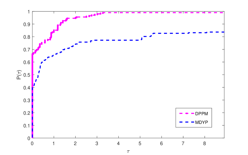
Figure 1: Performance profile with respect to number of iterations (ITER)

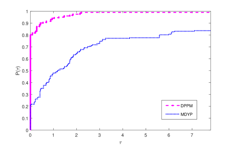
Figure 2: Performance profile with respect to number of function evaluations

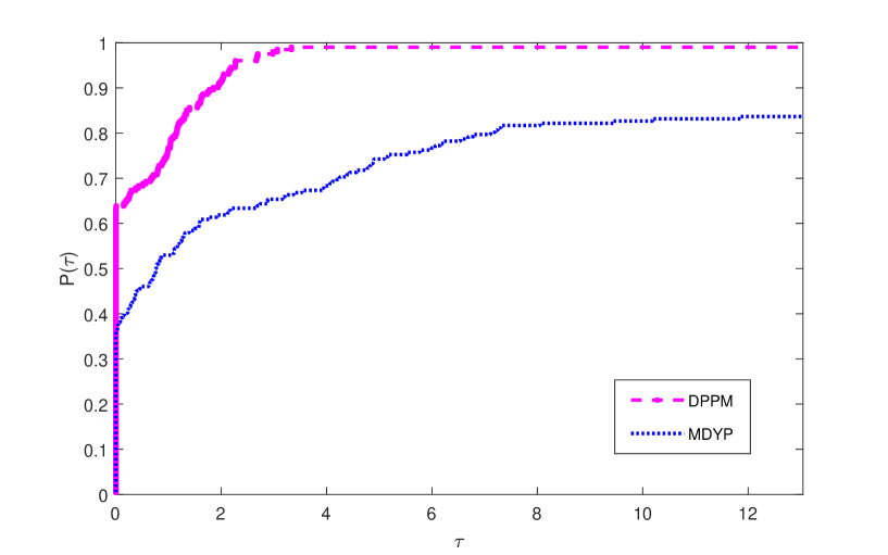
Figure 3: Performance profile with respect to CPU time

Table 2: Numerical Results for DPPM and MDYP for Problem 1 with given initial points and dimension

		DPPM				MDYP
DIM	INITIAL POINT	ITER	FVAL	TIME	NORM	ITER	FVAL	TIME	NORM
1000	$x_{1}$	38	82	0.39369	7.67E-06	33	161	0.11807	9.44E-06
	$x_{2}$	32	70	0.10322	7.15E-06	39	211	0.10552	9.40E-06
	$x_{3}$	120	252	0.32442	9.26E-06	49	256	0.70059	8.20E-06
	$x_{4}$	1	3	0.01260	0.00E+00	1	4	0.02221	0
	$x_{5}$	38	82	0.12030	8.15E-06	49	273	0.06990	8.50E-06
	$x_{6}$	37	79	0.04453	9.49E-06	57	311	0.06868	7.94E-06
	$x_{7}$	39	84	0.09649	8.57E-06	55	286	0.06015	7.37E-06
	$x_{8}$	37	80	0.11587	9.69E-06	56	291	0.09784	9.87E-06
5000	$x_{1}$	39	84	0.20890	8.86E-06	52	260	0.32704	7.10E-06
	$x_{2}$	32	69	0.35442	8.07E-06	32	186	0.16735	8.25E-06
	$x_{3}$	120	252	0.63706	9.26E-06	53	283	4.06230	9.09E-06
	$x_{4}$	1	3	0.02699	0.00E+00	1	4	0.19802	0
	$x_{5}$	39	84	0.33551	9.77E-06	54	308	0.34295	7.27E-06
	$x_{6}$	37	79	0.23014	9.48E-06	61	328	0.49383	9.07E-06
	$x_{7}$	41	88	0.27738	8.21E-06	46	245	0.32441	9.16E-06
	$x_{8}$	39	84	0.26216	9.78E-06	61	327	0.30915	8.09E-06
10000	$x_{1}$	40	86	0.36125	8.26E-06	42	208	0.30183	7.25E-06
	$x_{2}$	32	69	0.22630	9.73E-06	38	192	0.24845	7.01E-06
	$x_{3}$	120	252	1.21740	9.26E-06	53	283	10.89370	9.09E-06
	$x_{4}$	1	3	0.05100	0.00E+00	1	4	0.15397	0
	$x_{5}$	40	86	0.50858	9.29E-06	64	351	0.24912	8.09E-06
	$x_{6}$	37	79	0.30249	9.48E-06	42	216	0.79410	9.07E-06
	$x_{7}$	42	90	0.40105	7.71E-06	59	323	0.47751	8.01E-06
	$x_{8}$	40	86	0.34861	9.35E-06	78	434	0.59400	8.21E-06
50000	$x_{1}$	120	250	4.32320	9.72E-06	41	206	1.63900	6.58E-06
	$x_{2}$	34	73	0.77121	7.41E-06	33	164	1.38310	7.51E-06
	$x_{3}$	120	252	1.88700	9.26E-06	53	283	134.87960	9.09E-06
	$x_{4}$	1	3	0.26091	0.00E+00	1	4	2.40870	0
	$x_{5}$	55	117	2.36960	8.44E-06	69	386	3.03180	7.28E-06
	$x_{6}$	37	79	1.52390	9.49E-06	49	256	1.06890	9.47E-06
	$x_{7}$	55	117	1.79620	8.60E-06	66	398	3.07370	6.51E-06
	$x_{8}$	55	117	1.38480	8.44E-06	61	356	1.54750	7.43E-06
100000	$x_{1}$	156	323	6.91310	9.59E-06	63	321	2.36500	7.88E-06
	$x_{2}$	34	73	2.56550	8.93E-06	30	145	1.09880	8.96E-06
	$x_{3}$	120	252	4.15440	9.26E-06	53	283	460.82220	9.09E-06
	$x_{4}$	1	3	0.16653	0.00E+00	1	4	11.10340	0
	$x_{5}$	73	154	3.33150	9.20E-06	78	503	4.35460	9.93E-06
	$x_{6}$	37	79	1.37560	9.49E-06	50	259	3.27380	8.34E-06
	$x_{7}$	72	152	4.76270	9.88E-06	69	445	6.17050	9.63E-06
	$x_{8}$	73	154	3.36260	9.20E-06	59	345	3.37380	7.33E-06

Table 3: Numerical Results for DPPM and MDYP for Problem 2 with given initial points and dimension

		DPPM				MDYP
DIMENSION	INITIAL POINT	ITER	FVAL	TIME	NORM	ITER	FVAL	TIME	NORM
1000	$x_{1}$	2	5	0.01205	0.00E+00	13	40	0.036007	3.39E-06
	$x_{2}$	2	5	0.00846	0.00E+00	7	22	0.019472	5.13E-06
	$x_{3}$	12	25	0.091209	4.33E-06	8	25	0.080773	6.13E-06
	$x_{4}$	4	20	0.051613	0.00E+00	130	391	0.12599	6.48E-06
	$x_{5}$	9	19	0.026844	0.00E+00	6	19	0.016339	0.00E+00
	$x_{6}$	9	19	0.023649	9.24E-07	4	13	0.012304	0
	$x_{7}$	9	19	0.027893	0.00E+00	6	19	0.013595	0
	$x_{8}$	9	19	0.023562	0	6	19	0.011906	0.00E+00
5000	$x_{1}$	2	5	0.066537	0.00E+00	13	40	0.11026	7.50E-06
	$x_{2}$	2	5	0.022989	0.00E+00	8	25	0.068553	4.94E-06
	$x_{3}$	11	23	0.083563	9.62E-06	10	31	1.2681	3.78E-06
	$x_{4}$	3	18	0.04319	0.00E+00	455	1366	1.22	0
	$x_{5}$	11	23	0.15631	0.00E+00	6	19	0.01868	0.00E+00
	$x_{6}$	10	21	0.15303	2.04E-06	4	13	0.034344	0
	$x_{7}$	11	23	0.10842	0.00E+00	6	19	0.052581	0
	$x_{8}$	11	23	0.13773	0	6	19	0.045172	0.00E+00
10000	$x_{1}$	2	5	0.067238	0.00E+00	14	43	0.11068	2.89E-06
	$x_{2}$	2	5	0.064798	0.00E+00	8	25	0.088129	6.92E-06
	$x_{3}$	12	25	0.15601	4.61E-06	10	31	3.2523	5.11E-06
	$x_{4}$	3	18	0.13358	0.00E+00	821	2464	4.5746	8.32E-06
	$x_{5}$	11	23	0.20715	5.65E-06	6	19	0.13156	0.00E+00
	$x_{6}$	10	21	0.15698	6.69E-06	4	13	0.06196	0
	$x_{7}$	11	23	0.13313	5.65E-06	6	19	0.064923	0
	$x_{8}$	11	23	0.12422	5.65E-06	6	19	0.068141	0.00E+00
50000	$x_{1}$	23	50	1.2087	6.40E-06	14	43	0.60565	6.46E-06
	$x_{2}$	2	5	0.16224	0.00E+00	9	28	0.38936	1.05E-06
	$x_{3}$	11	23	0.51367	6.39E-06	10	31	27.959	5.37E-06
	$x_{4}$	3	18	0.36926	0.00E+00	f	f	f	f
	$x_{5}$	12	25	0.39204	6.62E-06	6	19	0.11452	0.00E+00
	$x_{6}$	12	25	0.74105	5.28E-07	4	13	0.073491	0
	$x_{7}$	12	25	0.50712	6.62E-06	6	19	0.11134	0
	$x_{8}$	12	25	0.59486	6.62E-06	6	19	0.2658	0.00E+00
100000	$x_{1}$	56	119	4.2791	7.39E-06	14	43	1.0548	9.13E-06
	$x_{2}$	2	5	0.35045	0.00E+00	9	28	0.56004	1.49E-06
	$x_{3}$	11	23	0.8678	8.25E-06	10	31	89.3792	5.41E-06
	$x_{4}$	3	18	0.65425	0.00E+00	f	f	f	f
	$x_{5}$	16	35	1.1296	9.42E-06	6	19	0.64241	0.00E+00
	$x_{6}$	12	25	0.75194	1.15E-06	4	13	0.38111	0
	$x_{7}$	16	35	1.5137	9.42E-06	6	19	0.48211	0
	$x_{8}$	16	35	1.0041	9.42E-06	6	19	0.57489	0.00E+00

Table 4: Numerical Results for DPPM and MDYP for Problem 3 with given initial points and dimension

		DPPM				MDYP
DIMENSION	INITIAL POINT	ITER	FVAL	TIME	NORM	ITER	FVAL	TIME	NORM
1000	$x_{1}$	9	20	0.012702	9.41E-06	12	39	0.028509	9.82E-06
	$x_{2}$	8	18	0.027765	8.11E-06	10	32	0.012253	9.57E-06
	$x_{3}$	7	16	0.03306	8.25E-06	9	29	0.081886	2.35E-06
	$x_{4}$	242	496	0.43655	9.42E-06	36	152	0.090671	4.38E-06
	$x_{5}$	10	22	0.018539	4.98E-06	37	210	0.070034	2.98E-06
	$x_{6}$	9	20	0.016934	3.23E-06	17	62	0.020589	6.28E-06
	$x_{7}$	10	22	0.016338	4.98E-06	37	210	0.072627	2.98E-06
	$x_{8}$	10	22	0.015586	5.00E-06	22	99	0.034992	2.15E-06
5000	$x_{1}$	10	22	0.10112	4.21E-06	13	42	0.058415	3.54E-06
	$x_{2}$	9	20	0.10815	3.63E-06	11	35	0.048767	3.71E-06
	$x_{3}$	7	16	0.046493	8.25E-06	9	29	1.1076	2.35E-06
	$x_{4}$	269	550	1.7034	9.31E-06	30	123	0.21588	3.44E-06
	$x_{5}$	11	24	0.08236	2.23E-06	36	209	0.37061	3.49E-06
	$x_{6}$	9	20	0.072288	3.24E-06	22	87	0.13458	6.38E-06
	$x_{7}$	11	24	0.14758	2.23E-06	36	209	0.50368	3.49E-06
	$x_{8}$	11	24	0.081127	2.23E-06	20	84	0.13688	8.44E-06
10000	$x_{1}$	10	22	0.14814	5.95E-06	13	42	0.12261	5.00E-06
	$x_{2}$	9	20	0.081035	5.13E-06	11	35	0.066221	5.24E-06
	$x_{3}$	7	16	0.067335	8.25E-06	9	29	3.1159	2.35E-06
	$x_{4}$	280	572	1.7613	9.79E-06	45	244	0.57493	7.67E-06
	$x_{5}$	11	24	0.053928	3.16E-06	31	177	0.39748	1.82E-06
	$x_{6}$	9	20	0.14158	3.24E-06	18	72	0.1053	8.19E-06
	$x_{7}$	11	24	0.16218	3.16E-06	31	177	0.27428	1.82E-06
	$x_{8}$	11	24	0.16983	3.16E-06	29	153	0.17573	6.17E-06
50000	$x_{1}$	43	92	2.0725	9.57E-06	14	45	0.52068	4.52E-06
	$x_{2}$	10	22	0.33935	2.29E-06	12	38	0.36153	4.63E-06
	$x_{3}$	7	16	0.14291	8.25E-06	9	29	22.695	2.35E-06
	$x_{4}$	307	626	7.8832	9.69E-06	38	174	1.9062	9.53E-06
	$x_{5}$	17	37	0.36148	4.12E-06	44	295	9.8907	6.42E-06
	$x_{6}$	9	20	0.13877	3.24E-06	23	90	8.835	6.56E-06
	$x_{7}$	17	37	0.34472	4.12E-06	44	295	9.8494	6.41E-06
	$x_{8}$	17	37	0.79731	4.12E-06	36	222	2.2409	4.06E-06
100000	$x_{1}$	58	123	4.0543	7.82E-06	14	45	0.63779	6.39E-06
	$x_{2}$	10	22	1.0512	3.24E-06	12	38	0.46115	6.55E-06
	$x_{3}$	7	16	0.59808	8.25E-06	9	29	87.9961	2.35E-06
	$x_{4}$	319	650	15.465	9.35E-06	33	147	3.2193	7.98E-06
	$x_{5}$	32	69	2.4051	9.29E-06	34	224	3.9158	4.61E-06
	$x_{6}$	9	20	0.70022	3.24E-06	21	81	10.7951	4.64E-06
	$x_{7}$	32	69	2.3197	9.29E-06	34	224	4.1301	4.61E-06
	$x_{8}$	32	69	2.5293	9.29E-06	37	225	2.6843	4.58E-06

Table 5: Numerical Results for DPPM and MDYP for Problem 4 with given initial points and dimension

		DPPM				MDYP
DIMENSION	INITIAL POINT	ITER	FVAL	TIME	NORM	ITER	FVAL	TIME	NORM
1000	$x_{1}$	1	3	0.006994	0.00E+00	f	f	f	f
	$x_{2}$	5	11	0.016786	0.00E+00	f	f	f	f
	$x_{3}$	9	19	0.024407	1.87E-06	304	913	3.7303	9.98E-06
	$x_{4}$	185	382	1.0441	0.00E+00	f	f	f	f
	$x_{5}$	11	23	0.058111	9.06E-06	f	f	f	f
	$x_{6}$	19	40	0.074199	6.95E-06	856	2569	2.6683	1.00E-05
	$x_{7}$	11	23	0.042337	9.06E-06	f	f	f	f
	$x_{8}$	24	50	0.14774	4.23E-06	f	f	f	f
5000	$x_{1}$	1	3	0.020524	0.00E+00	f	f	f	f
	$x_{2}$	5	11	0.090725	0.00E+00	f	f	f	f
	$x_{3}$	9	19	0.090678	1.87E-06	304	913	24.0402	9.98E-06
	$x_{4}$	203	418	2.2173	0.00E+00	870	2612	22.9668	9.99E-06
	$x_{5}$	13	27	0.26952	4.42E-06	f	f	f	f
	$x_{6}$	19	40	0.32377	7.56E-06	918	2755	5.3977	9.98E-06
	$x_{7}$	13	27	0.35444	4.42E-06	f	f	f	f
	$x_{8}$	25	52	0.42654	3.97E-06	f	f	f	f
10000	$x_{1}$	1	3	0.026783	0.00E+00	f	f	f	f
	$x_{2}$	5	11	0.15274	0.00E+00	f	f	f	f
	$x_{3}$	9	19	0.092308	1.87E-06	304	913	64.261	9.98E-06
	$x_{4}$	211	434	2.9705	0.00E+00	f	f	f	f
	$x_{5}$	13	27	0.53653	2.93E-06	f	f	f	f
	$x_{6}$	19	40	0.76099	7.49E-06	921	2764	8.8082	9.99E-06
	$x_{7}$	13	27	0.37658	2.93E-06	f	f	f	f
	$x_{8}$	25	52	0.80643	5.62E-06	f	f	f	f
50000	$x_{1}$	1	3	0.13612	0.00E+00	f	f	f	f
	$x_{2}$	5	11	0.75059	0.00E+00	f	f	f	f
	$x_{3}$	9	19	0.64213	1.87E-06	304	913	750.0724	9.98E-06
	$x_{4}$	229	470	13.7584	0.00E+00	f	f	f	f
	$x_{5}$	11	24	1.5439	2.13E-06	f	f	f	f
	$x_{6}$	19	40	1.8662	7.45E-06	921	2764	35.4218	1.00E-05
	$x_{7}$	11	24	0.89235	2.13E-06	f	f	f	f
	$x_{8}$	11	24	0.69469	2.12E-06	f	f	f	f
100000	$x_{1}$	1	3	0.17122	0.00E+00	f	f	f	f
	$x_{2}$	5	11	1.2485	0.00E+00	f	f	f	f
	$x_{3}$	9	19	0.73873	1.87E-06	304	913	2739.78	9.98E-06
	$x_{4}$	237	486	28.0708	0.00E+00	f	f	f	f
	$x_{5}$	15	33	2.7825	1.35E-06	f	f	f	f
	$x_{6}$	19	40	2.4742	7.45E-06	921	2764	73.568	1.00E-05
	$x_{7}$	15	33	3.0101	1.35E-06	f	f	f	f
	$x_{8}$	15	33	1.8552	1.35E-06	f	f	f	f

Table 6: Numerical Results for DPPM and MDYP for Problem 4 with given initial points and dimension

		DPPM				MDYP
DIMENSION	INITIAL POINT	ITER	FVAL	TIME	NORM	ITER	FVAL	TIME	NORM
1000	$x_{1}$	20	44	0.019887	7.58E-06	11	38	0.025455	3.21E-06
	$x_{2}$	8	18	0.022029	8.00E-06	9	29	0.009151	8.71E-06
	$x_{3}$	12	27	0.028013	4.40E-06	12	40	0.12209	1.70E-06
	$x_{4}$	1	3	0.004682	0.00E+00	1	4	0.014134	0
	$x_{5}$	17	37	0.035034	5.83E-06	21	79	0.031607	6.66E-06
	$x_{6}$	14	31	0.017107	8.77E-06	11	36	0.02408	3.32E-06
	$x_{7}$	17	37	0.042426	5.83E-06	21	79	0.028564	6.66E-06
	$x_{8}$	17	37	0.051895	5.84E-06	17	61	0.023712	6.86E-06
5000	$x_{1}$	21	46	0.18004	8.27E-06	11	38	0.040818	7.19E-06
	$x_{2}$	9	20	0.084557	3.58E-06	10	32	0.044893	8.33E-06
	$x_{3}$	12	27	0.099041	4.40E-06	12	40	1.7057	1.70E-06
	$x_{4}$	1	3	0.025493	0.00E+00	1	4	0.16941	0
	$x_{5}$	23	50	0.17716	5.38E-06	19	69	0.095303	2.22E-06
	$x_{6}$	14	31	0.22375	8.76E-06	11	36	0.058293	3.32E-06
	$x_{7}$	23	50	0.31409	5.38E-06	19	69	0.065043	2.22E-06
	$x_{8}$	23	50	0.14158	5.38E-06	27	122	0.17497	3.72E-06
10000	$x_{1}$	22	48	0.24683	5.71E-06	12	41	0.21346	4.72E-06
	$x_{2}$	9	20	0.08746	5.06E-06	11	35	0.09006	1.49E-06
	$x_{3}$	12	27	0.051866	4.40E-06	12	40	3.8951	1.70E-06
	$x_{4}$	1	3	0.018948	0.00E+00	1	4	0.55884	0
	$x_{5}$	23	50	0.20947	7.61E-06	17	62	0.16185	9.13E-06
	$x_{6}$	14	31	0.19068	8.76E-06	11	36	0.061976	3.32E-06
	$x_{7}$	23	50	0.2562	7.61E-06	17	62	0.13079	9.13E-06
	$x_{8}$	23	50	0.31204	7.61E-06	29	114	0.66644	9.92E-06
50000	$x_{1}$	74	156	2.2287	8.50E-06	13	44	0.34412	7.07E-07
	$x_{2}$	10	22	0.59981	2.26E-06	11	35	0.24221	3.33E-06
	$x_{3}$	12	27	0.30703	4.40E-06	12	40	28.6017	1.70E-06
	$x_{4}$	1	3	0.12101	0.00E+00	1	4	2.2182	0
	$x_{5}$	32	69	0.69063	7.53E-06	18	65	0.19135	8.62E-06
	$x_{6}$	14	31	0.30697	8.76E-06	11	36	0.38975	3.32E-06
	$x_{7}$	32	69	1.7399	7.53E-06	18	65	0.44778	8.62E-06
	$x_{8}$	32	69	0.96137	7.53E-06	18	65	0.37787	8.97E-06
100000	$x_{1}$	97	203	4.8452	8.54E-06	13	44	0.75655	1.00E-06
	$x_{2}$	10	22	0.43113	3.20E-06	11	35	0.4291	4.71E-06
	$x_{3}$	12	27	0.83201	4.40E-06	12	40	115.0905	1.70E-06
	$x_{4}$	1	3	0.39874	0.00E+00	1	4	8.6205	0
	$x_{5}$	43	92	2.8254	8.61E-06	19	68	1.1444	2.35E-06
	$x_{6}$	14	31	1.1267	8.76E-06	11	36	0.38034	3.32E-06
	$x_{7}$	43	92	2.3561	8.61E-06	19	68	1.0552	2.35E-06
	$x_{8}$	43	92	2.8962	8.61E-06	19	68	0.70571	2.41E-06

Figures 1-3 shows the Dolan and Mor$\acute{e}$ [3] performance profiles based on the number of iterations, the number of functions evaluations, and CPU time.

It can be observed from Figure 1 , DPPM solves and wins almost $70\%$, while MSDY solves and wins less than $50\%$ of the $200$ problems. In terms of the number of function evaluation Figure 2 shows that DPPM outperforms MDYP, as it solves about $80\%$ of the problems with the least number of functions evaluation. This good performance of SSGM2 is related to the efficiency of its search direction since it requires less function evaluation for computing the accepted steplength.

In terms of the CPU time metric, DPPM is faster than MDYP with more than $60\%$ success. In summary, the proposed DPPM method is more successful than MDYP method based on the numerical experiments presented. This is due to the improvement in the search direction.

5.   Conclusions and Future Research

We proposed a diagonal Polak-Ribi$\grave{e}$re-Polyk (PRP) type projection method for solving convex constrained nonlinear monotone equations problems (DPPM). The proposed method requires neither the exact Jacobian computation nor its storage space. This is an advantage, especially for large-scale nonsmooth problems. The global convergence of the proposed method is obtained without any merit function or differentiability assumptions on the residual function. Moreover, we proposed a simple strategy for ensuring that the components of the diagonal matrices are safely positive at each iteration.

In future research, we intend to study better techniques to use for improving the search direction with a suitable line search strategy. Because of the low memory requirement of the DPPM method, we hope it will perform well when applied to solve practical problems arising from compressed sensing and image processing this is also another subject for future research.

Appendix

In this section we list the test problems used for the numerical experiments.
Problem 1 [14] Modified Exponential Function

$$F_{1}(x) =e^{x_{1}}-1,$$

$$F_{i}(x) =e^{x_{i}}-x(i-1)-1,~{}\text{for }i=2,3,...,n.$$

and $$\Omega=R_{+}^{n}.$$

Problem 2 [14] Modified Logarithmic Function

$$F_{i}(x) =\ln(|x_{i}|+1)-\frac{x_{i}}{n},~{}\text{for }i=2,3,...,n.$$

and $$\Omega=R_{+}^{n}.$$

Problem 3 Nonsmooth Function [41]

$$F_{i}(x) =2x_{i}-\sin|x_{i}|,~{}i=1,2,3,...,n.$$

and $$\Omega=R_{+}^{n}.$$

Problem 4[13]

$$F_{i}(x) =\min(\min(|x_{i}|,x_{i}^{2}),\max(|x_{i}|,x_{i}^{3})),~{}i=1,2,3,...,n.$$

and $$\Omega=R_{+}^{n}.$$

Problem 5 [14] Strictly Convex Function

$$F_{i}(x) =e^{x_{i}}-1,~{}\text{for }i=1,2,...,n.$$

and $$\Omega=R_{+}^{n}.$$

References

- [1] Abubakar, A. B., and Kumam, P. A descent Dai-Liao conjugate gradient method for nonlinear equations. Numerical Algorithms, https://doi.org/10.1007/s11075–018–0541–z.
- [2] Cheng, W. A PRP type method for systems of monotone equations. Mathematical and Computer Modelling 50, 1-2 (2009), 15–20.
- [3] Dolan, E. D., and Moré, J. J. Benchmarking optimization software with performance profiles. Mathematical Programming 91, 2 (2002), 201–213.
- [4] Dong, X. L., Liu, H., Xu, Y. L., and Yang, X. M. Some nonlinear conjugate gradient methods with sufficient descent condition and global convergence. Optimization Letters 9, 7 (2015), 1421–1432.
- [5] Eshaghnezhad, M., Effati, S., and Mansoori, A. A neurodynamic model to solve nonlinear pseudo-monotone projection equation and its applications. IEEE Transactions on Cybernetics 47, 10 (2017), 3050–3062.
- [6] Fukushima, M. Equivalent differentiable optimization problems and descent methods for asymmetric variational inequality problems. Math. Program. 53, 1-3 (1992), 99–110.
- [7] Ghaddar, B., Marecek, J., and Mevissen, M. Optimal power flow as a polynomial optimization problem. IEEE Transactions on Power Systems 31, 1 (2016), 539–546.
- [8] Gu, B., Sheng, V. S., Tay, K. Y., Romano, W., and Li, S. Incremental support vector learning for ordinal regression. IEEE Transactions on Neural networks and learning systems 26, 7 (2015), 1403–1416.
- [9] Han, L., Yu, G., and Guan, L. Multivariate spectral gradient method for unconstrained optimization. Applied Mathematics and Computation 201, 1-2 (2008), 621–630.
- [10] Hu, Y., and Wei, Z. Wei–Yao–Liu conjugate gradient projection algorithm for nonlinear monotone equations with convex constraints. International Journal of Computer Mathematics 92, 11 (2015), 2261–2272.
- [11] Iusem, N. A., and Solodov, V. M. Newton-type methods with generalized distances for constrained optimization. Optimization 41, 3 (1997), 257–278.
- [12] La Cruz, W. A projected derivative-free algorithm for nonlinear equations with convex constraints. Optimization Methods and Software 29, 1 (2014), 24–41.
- [13] La Cruz, W. A spectral algorithm for large-scale systems of nonlinear monotone equations. Numerical Algorithms 76, 4 (2017), 1109–1130.
- [14] La Cruz, W., Martínez, J., and Raydan, M. Spectral residual method without gradient information for solving large-scale nonlinear systems of equations. Mathematics of Computation 75, 255 (2006), 1429–1448.
- [15] Li, J., Li, X., Yang, B., and Sun, X. Segmentation-based image copy-move forgery detection scheme. IEEE Transactions on Information Forensics and Security 10, 3 (2015), 507–518.
- [16] Li, Q., and Li, D. H. A class of derivative-free methods for large-scale nonlinear monotone equations. IMA Journal of Numerical Analysis 31, 4 (2011), 1625–1635.
- [17] Liu, J., and Du, X. L. A gradient projection method for the sparse signal reconstruction in compressive sensing. Applicable Analysis (2017), 1–10.
- [18] Liu, J., and Duan, Y. Two spectral gradient projection methods for constrained equations and their linear convergence rate. Journal of Inequalities and Applications 2015, 1 (2015), 8.
- [19] Liu, J., and Li, S. Multivariate spectral DY-type projection method for convex constrained nonlinear monotone equations. Journal of Industrial & Management Optimization 13, 1 (2017), 283–295.
- [20] Liu, J. K., and Li, S. A projection method for convex constrained monotone nonlinear equations with applications. Computers and Mathematics with Applications 70, 10 (2015), 2442–2453.
- [21] Liu, S., Huang, Y., and Jiao, H. W. Sufficient descent conjugate gradient methods for solving convex constrained nonlinear monotone equations. Abstract and Applied Analysis 2014 (2014), 1–12.
- [22] Ma, F., and Wang, C. Modified projection method for solving a system of monotone equations with convex constraints. Journal of Applied Mathematics and Computing 34, 1 (2010), 47–56.
- [23] Mohammad, H., and Abubakar, A. B. A positive spectral gradient-like method for nonlinear monotone equations. Bulletin of Computational and Applied Mathematics 5, 1 (2017), 97–113.
- [24] Ou, Y., and Li, J. A new derivative-free SCG-type projection method for nonlinear monotone equations with convex constraints. Journal of Applied Mathematics and Computing 56, 1 (2018), 195–216.
- [25] Ou, Y., and Liu, Y. Supermemory gradient methods for monotone nonlinear equations with convex constraints. Computational and Applied Mathematics 36, 1 (2017), 259–279.
- [26] Papp, Z., and Rapajić, S. FR type methods for systems of large-scale nonlinear monotone equations. Applied Mathematics and Computation 269 (2015), 816–823.
- [27] Qian, G., Han, D., Xu, L., and Y., H. Solving nonadditive traffic assignment problems: A self-adaptive projection-auxiliary problem method for variational inequalities. Journal of Industrial & Management Optimization 9, 1 (2013), 255–274.
- [28] Solodov, M. V., and Svaiter, B. A globally convergent inexact Newton method for systems of monotone equations. In Reformulation: Nonsmooth, Piecewise Smooth, Semismooth and Smoothing Methods. Springer, 1998, pp. 355–369.
- [29] Sun, M., and Liu, J. Three derivative-free projection methods for nonlinear equations with convex constraints. Journal of Applied Mathematics and Computing 47, 1-2 (2015), 265–276.
- [30] Wang, C., and Wang, Y. A superlinearly convergent projection method for constrained systems of nonlinear equations. Journal of Global Optimization 44, 2 (2009), 283–296.
- [31] Wang, C., Wang, Y., and Xu, C. A projection method for a system of nonlinear monotone equations with convex constraints. Mathematical Methods of Operations Research 66, 1 (2007), 33–46.
- [32] Wang, X., Li, S., and Kou, X. A self-adaptive three-term conjugate gradient method for monotone nonlinear equations with convex constraints. Calcolo 53, 2 (2016), 133–145.
- [33] Wood, A. J., and Wollenberg, B. F. Power generation, operation, and control. John Wiley & Sons, 2012.
- [34] Xiao, Y., and Zhu, H. A conjugate gradient method to solve convex constrained monotone equations with applications in compressive sensing. Journal of Mathematical Analysis and Applications 405, 1 (2013), 310–319.
- [35] Yan, Q., Peng, X. Z., and Li, D. H. A globally convergent derivative-free method for solving large-scale nonlinear monotone equations. Journal of Computational and Applied Mathematics 234, 3 (2010), 649–657.
- [36] Yu, G., Niu, S., and Ma, J. Multivariate spectral gradient projection method for nonlinear monotone equations with convex constraints. Journal of Industrial and Management Optimization 9, 1 (2013), 117–129.
- [37] Yu, Z., Lin, J., Sun, J., Xiao, Y. H., Liu, L., and Li, Z. H. Spectral gradient projection method for monotone nonlinear equations with convex constraints. Applied Numerical Mathematics 59, 10 (2009), 2416–2423.
- [38] Yuan, N. A derivative-free projection method for solving convex constrained monotone equations. SCIENCEASIA 43, 3 (2017), 195–200.
- [39] Zhang, M., Xiao, Y., and Dou, H. Solving nonlinear constrained monotone equations via limited memory BFGS algorithm. Journal of Computational Information Systems 7, 11 (2011), 3995–4006.
- [40] Zheng, Y., Jeon, B., Xu, D., Wu, Q. M., and Zhang, H. Image segmentation by generalized hierarchical fuzzy c-means algorithm. Journal of Intelligent & Fuzzy Systems 28, 2 (2015), 961–973.
- [41] Zhou, W., and Li, D. H. Limited memory BFGS method for nonlinear monotone equations. Journal of Computational Mathematics (2007), 89–96.
- [42] Zhou, W., and Wang, F. A PRP-based residual method for large-scale monotone nonlinear equations. Applied Mathematics and Computation 261 (2015), 1–7.