Optimal control of the mean field equilibrium for a pedestrian tourists’ flow model

Abstract

Art heritage cities are popular tourist destinations but for many of them overcrowding is becoming an issue. In this paper, we address the problem of modeling and analytically studying the flow of tourists along the narrow alleys of the historic center of a heritage city. We initially present a mean field game model, where both continuous and switching decisional variables are introduced to respectively describe the position of a tourist and the point of interest that he/she may visit. We prove the existence of a mean field equilibrium. A mean field equilibrium is Nash-type equilibrium in the case of infinitely many players. Then, we study an optimization problem for an external controller who aims to induce a suitable mean field equilibrium.

1 Introduction

In the recent years, art heritage cities have experienced a continuous growth of tourists’ flow, to the point that overcrowding is becoming an issue, and local authorities start implementing countermeasures. In this paper we address the problem of modeling and analytically studying the flow of tourists (or, more precisely, of daily pedestrian excursionists) along the narrow alleys of the historic center of a heritage city. Starting from the contents of Bagagiolo and Pesenti (2017), we recast those results into a mean field game with controlled dynamics on a network, representing the attractive sites in the city and the possible paths to reach them.

We here assume for simplicity that tourists have only two main attractions to visit, as a context with more attractions can be equally treated. We represent possible paths as a circular network containing three nodes: the train station $S$ where tourists arrive in the morning and to which they have to return in the evening; the first attraction $P_{1}$; the second attraction $P_{2}$ (see Figure 1.a). The arrival flow at the station is exhogenous, given by a continuous function $g:[0,T]\to[0,+\infty[$ representing, roughly speaking, the density of arriving tourists per unit of time. The time by which everyone has to be returned to the station after the tour is the final horizon $T>0$.

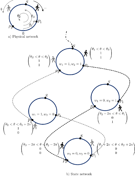
Figure 1: a) the physical network of the paths inside the city, counterclockwise positively oriented (with the three identified points: train station, $S$, and two attractions, $P_{1},P_{2}$) and two tourists visiting the city following opposite directions. b) the state network and the states $(\theta,w_{1},w_{2})$ of the tourists during their visits. Each singular circle-branch represents the network of the city paths as seen by tourist with given values of the switching variables $w_{1},w_{2}$. The dashed arrows between the four circles-branches represent the switching of the four labels: at the beginning the label is $(1,1)$; when the attraction $P_{1}$ is reached (and hence visited), the label switches to $(0,1)$, and similarly when $P_{2}$ is reached; the last is $(0,0)$ which holds when both attractions are reached. The point-dashed arrow represents the external arrival flow in the station.

A single tourist (agent), starting at position $\theta$ at time $t$, controls its own dynamics, represented by the equation

$$\begin{cases}\theta^{\prime}(s)=u(s),&s\in]{t},T]\\ \theta(t)=\theta&\end{cases}$$ (1)

where $\theta(s)\in\mathbb{R}$ is the space-coordinate in the network, and $s\mapsto u(s)\in\mathbb{R}$ is a measurable and locally integrable control, namely $u\in L^{1}_{loc}(t,T)$. We represent the network by a circle (see Figure 1), and we denote with $\theta_{S}$, $\theta_{1}$ and $\theta_{2}$ respectively the position of the station, and of the attractions $P_{1}$ and $P_{2}$. In particular, we assume that

$${0<\theta_{1}<\theta_{S}<\theta_{2}<2\pi,}$$ (2)

which is not restrictive due to the circularity representation of the state space. Moreover (see Figure 1 and Figure 2), when convenient, we will identify $\theta$ and $\theta\pm 2\pi$.

To each tourist, we associate a time-varying label $(w_{1},w_{2})\in\{0,1\}\times\{0,1\}$. For $i\in\{1,2\}$, $w_{i}(t)=1$ means that, at the time $t$, the attraction $P_{i}$ has not been visited yet, and $w_{i}(t)=0$ that the attraction has been already visited. The state of an agent is then represented by the triple $(\theta,w_{1},w_{2})$, where $\theta$ is a time-continuous variable and $w_{1},w_{2}$ are switching variables. In the following, we denote by $B=[0,2\pi]\times\{0,1\}\times\{0,1\}$ the state space of variables $(\theta,w_{1},w_{2})$, and in particular we call (circle) branch any subset $B_{{w}_{1},{w}_{2}}$ of $B$ which includes the states $(\theta,{{w}_{1},{w}_{2}})$, with $(w_{1},w_{2})$ fixed and $\theta$ varying in $[0,2\pi].$ Such branches correspond to edges of the switching networks in Figure 2, which represents the network of Figure 1 in an equivalent way.

While the evolution of $\theta$ is governed by (1), switching variables can only evolve from $1$ to $0$, that is

$$w_{i}=\begin{cases}1&\text{for}\ s\in[t,\tau_{i}]\\ 0&\text{for}\ s\in]\tau_{i},T],\end{cases}$$

with $\tau_{i}\in[t,T]$ the first instant at which the agent reaches and visits attraction $P_{i}$, $i\in\{1,2\}$. This evolution is represented by the arrows and the labels in Figure 1.b (see also Figure 2). To exemplify, consider in Figure 1.b an agent that arrives at the station and visits $P_{1}$ first: its initial state is $(\theta_{S},1,1)\in B_{1,1}$; at $\tau_{1}\in[0,T]$, $w_{1}$ switches from 1 to 0 so that, immediately after $\tau_{1}$, the tourist’s state $(\theta,0,1)$ belongs to the branch $B_{0,1}$ (see also Figure 2).

The cost to be minimized by every agent takes into account: i) the hassle of running during the tour; ii) the pain of being entrapped in highly congested paths; iii) the frustration of not being able to visit some attractions; iv) the disappointment of not being able to reach the station by the final horizon $T$. Such a cost can be analytically represented by

$$\begin{array}[]{ll}J(u;t,\theta,w_{1},w_{2})=\int_{t}^{T}\left(\frac{u(s)^{2}}{2}+\mathcal{F}^{w_{1}(s),w_{2}(s)}(\mathcal{M}(s))\right)ds+&\\ \ \ \ \ \ \ \ \ \ \ \ \ \ \ \ \ \ \ \ \ \ \ +c_{1}w_{1}(T)+c_{2}w_{2}(T)+c_{S}\xi_{\theta=\theta_{S}}(T)&\end{array}$$ (3)

Here, $c_{1},c_{2},c_{S}>0$ are fixed, and $\xi_{\theta=\theta_{S}}(s)\in\{0,1\}$ and it is equal to $0$ if and only if $\theta(s)=\theta_{S}$. In (3), the quadratic term inside the integral stands for cost i) while the other term stands for the congestion cost ii); the following two addenda stand for costs iii); the last addendum stands for cost iv). In particular, the congestion cost $\mathcal{F}^{w_{1}(s),w_{2}(s)}(\mathcal{M}(s))$ is instantaneously paid by an agent whose switching label at time $s$ is $(w_{1}(s),w_{2}(s))$, being $\mathcal{M}(s)$ the actual distribution of the agents. For any $(w_{1},w_{2})\in\{0,1\}\times\{0,1\}$, $\mathcal{F}^{w_{1},w_{2}}$ is a positive function defined on the set of all admissible distribution of agents.

The problem here treated differs from that in Bagagiolo and Pesenti (2017) in the respect that the discontinuous final cost $c_{S}\xi_{\theta=\theta_{S}}(T)$ in (3) is replaced by a smooth cost $c_{3}(\theta-\theta_{S})^{2}$. As done in Bagagiolo and Pesenti (2017), the problem is considered as a mean field game, and the existence of a mean field equilibrium is proven under suitable assumptions. A mean field equilibrium is a time-varying distribution of agents on the network, $s\mapsto\mathcal{M}^{*}(s)$ for $s\in[0,T]$ generating, when plugged in (3), an optimal control $u^{*}$ and associated optimal trajectory, for any agent starting at the station at time $t\in[0,T]$, yielding again the time-varying distribution $\mathcal{M}^{*}$. A mean field equilibrium can be seen as a fixed point, over a suitable set of time-varying distributions, of a map of the form

$$\mathcal{M}\longrightarrow u_{\mathcal{M}}\longrightarrow\mathcal{M}_{u_{\mathcal{M}}}$$ (4)

where $u_{\mathcal{M}}$ is the optimal control when $\mathcal{M}$ is inserted in (3), and $\mathcal{M}_{u_{\mathcal{M}}}$ is the corresponding evolution of the agents’ distribution when all of them are moving implementing $u_{\mathcal{M}}$ as control. Of course, the problem must be coupled with an initial condition for the distribution $\mathcal{M}$, whereas the boundary condition is represented by the incoming flow $g$.

We remark that the concept of mean field equilibrium is of Nash type. Indeed, in the case of a large number of agents (even infinitely many, as in the case of a mean field game) every single agent is irrelevant, the single agent has measure zero, it is lost in the crowd. Hence, at equilibrium, for a single agent is not convenient to unilaterally change behavior, because such a single choice will not change the mean field $\mathcal{M}$, and the agent will not optimize his behavior.

That said, the goal of the present paper is twofold. First we amend some stringent assumptions that were made in Bagagiolo and Pesenti (2017) to prove the existence of a mean field equilibrium. Then, we study a possible optimization problem for an external controller who aims to induce a suitable mean field equilibrium. We suppose that the external controller (the city administration, for example) may act on the congestion functions $\mathcal{F}^{w_{1},w_{2}}$, choosing them among a suitable set of admissible functions.

We also note that the presence of a discontinuous final cost is by-passed using a characterization of the value function at some significant states, identifying at the same time a finite set of optimal controls.

Consider as an example the historical center of the city of Venice, Italy. Tourists typically enter the city at the train station and from there they have two main routes, a shorter and a longer one, to major monuments. In recent years, the shorter route has been particularly congested on peak days. For this reason, local authorities have introduced both some gates to slow down the access to the shorter route and some street signs to divert at least part of the tourist flow along the longer route.

Mean field games theory goes back to the seminal work by Lasry and Lions (2006) (see also Huang et al. (2006)), where the new standard terminology of mean field games was introduced. This theory includes methods and techniques to study differential games with a large population of rational players and it is based on the assumption that the population influences the individuals’ strategies through mean field parameters. Several application domains such as economic, physics, biology and network engineering accommodate mean field game theoretical models (Achdou et al., 2012; Lachapelle et al., 2010). In particular, models to the study of dynamics on networks and/or pedestrian movement are proposed, for example, by Camilli et al. (2015), by Cristiani et al. (2015), by Camilli et al. (2017), and by Bagagiolo et al. (2017).

Very recently Lasry and Lions (2018) have introduced a new class of mean field games to model situations involving one dominant agent and a large group of small players. Our work can be framed in this new class when it deals with the possible role of local authorities in the optimization of tourist flows.

The problem here treated is also a routing problem (for a particular case of pedestrian movement with possible multiple destinations see, for example, Hoogendoorn and Bovy (2005)). Note that different strategies were proposed to control the roadway congestion, such as variable speed limits (Hegyi et al., 2005), ramp metering (Gomes and Horowitz, 2006) or signal control (“Brian” Park et al., 2009). However, such mechanisms neither consider the agents’ perspective, nor affect the total amount of vehicles/people. A significant research effort was done to understand the agents’ answer to external communications from intelligent traveler information devices (Khattak et al., 1996; Srinivasan and Mahmassani, 2000) and, in particular, to study the effect of such technologies on the agents’ choice and on the dynamical properties of the transportation network (Como et al., 2013). Moreover it is well known that when individual agents make their routing decisions to minimize their own experienced delays, then the overall network congestion is considerably higher than the congestion resulting from a central planner directing traffic explicitly (Pigou, 1920). From that the idea to include in our problem an external controller inducing a suitable mean field equilibrium.

Note also that in the specific case of vehicular congestion, tolls payment is considered to influence drivers to make routing choices that result in globally optimal routing, namely to force the Wardrop equilibrium to align with the system optimum network flow (Smith, 1979; Morrison, 1986; Dial, 1999; Cole et al., 2006). The Wardop equilibrium, proposed by Wardrop (1952), is a configuration in which the perceived cost associated to any source-destination path chosen by a nonzero fraction of drivers does not exceed the perceived cost associated to any other path. This is a stationary concept, whose continuous counterpart was recently developed by Carlier et al. (2008) and by Carlier and Santambrogio (2012).

Not only does the latter fit the situation of pedestrian congestion but also is useful to analyse large-scale traffic problems, in which one only wants to identify the average value of the traffic congestion in different zones of a large area. Actually, also the models using that continuous framework are essentially stationary, as they only account for a sort of cyclical movement, where every path is constantly occupied by the same density of vehicles, since those reaching the destination are immediately replaced by others. This is the essential difference with respect to the mean field models. Indeed in the latter, due to the explicit presence of time, the optimal evolution is given by a system coupling a transport equation and an Hamilton-Jacobi equation.

2 Preliminary results

As anticipated in the introduction, the problem here treated differs from that in Bagagiolo and Pesenti (2017), under the respect that the final cost $c_{S}\xi_{\theta=\theta_{S}}(T)$ in (3) replaces the smooth cost $c_{3}(\theta-\theta_{S})^{2}$ of Bagagiolo and Pesenti (2017). Hence, we here recall some of the results from the previous paper that still hold true in our case, and present some new ways to approach the problem.

We define the value function $V(\theta,t,w_{1},w_{2})$ as the infimum over the measurable controls of the cost (3) faced by an agent starting its evolution at the state $(\theta,w_{1},w_{2})$, at time $t$, that is

$$V(\theta,t,w_{1},w_{2})=\inf_{u\in L^{1}_{loc}(t,T)}J(u;t,\theta,w_{1},w_{2})$$

Note that when the distributional evolution $t\mapsto\mathcal{M}(t)$, i.e. the density of the agents, is initially given, then $V$ does not depend on $\mathcal{M}$. As well as in Bagagiolo and Pesenti (2017), the following two sets of equations are considered:

• the set of Hamilton-Jacobi-Bellman equations (one for each branch $B_{w_{1},w_{2}}$) associated to the problem, and fully described through (26) in Appendix B (corresponding to equations (3)–(6) in Bagagiolo and Pesenti (2017));

• the associated set of transport equations (one for each branch), fully described through (27) in Appendix B (corresponding to equations (8a)–(8d) in Bagagiolo and Pesenti (2017)).

Regarding (a), note that in (26) boundary conditions are given by the value, at the switching points, of the solution in the consecutive branch. This fact comes from the dynamic programming principle, and from interpreting the optimal control problem on a single branch as an exit-time problem (Bagagiolo and Danieli, 2012). More in detail (see Figure 2), the exit cost from $B_{1,1}$ at time $\tau$ is given by $V(\theta_{1},\tau,0,1)$ at $\theta_{1}$, and by $V(\theta_{2},\tau,1,0)$ at $\theta_{2}$. The exit costs from $B_{0,1}$ and from $B_{1,0}$ are, respectively, $V(\theta_{2},\tau,0,0)$ and $V(\theta_{1},\tau,0,0)$ (on both exit points of the branch). On the final branch $B_{0,0}$ the problem is reduced to reaching the station at the least cost within the final time $T$.

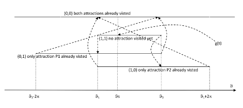
Figure 2: Switching cross branches representation

Note also that, when the distribution $\mathcal{M}$ is given, the optimal control problem faced by an agent on a branch is a rather standard combination of a reaching target (the station) problem and suitable exit time problems. In particular, the optimal control problem on $B_{0,0}$ can be solved, and $V(\cdot,\cdot;0,0)$ calculated, independently from the evolution of the system on the other branches. Once the problem on $B_{0,0}$ is solved, one may proceed backwards and solve the problems on $B_{0,1}$ and $B_{1,0}$ and, eventually, on $B_{1,1}$.

Regarding (b), the transport equations (27) are solved, for every $(w_{1},w_{2})\in\{0,1\}^{2}$ and for every $t\in[0,T]$, by a time dependent measure $m^{w_{1},w_{2}}(\cdot,t):[0,2\pi]\to[0,+\infty[$ representing the agents’ distribution on the branch $B_{w_{1},w_{2}}$ at time $t$. It is assumed that the city network is initially empty of tourist, that is, $m^{w_{1},w_{2}}(\cdot,0)=0$ for $(w_{1},w_{2})\in\{0,1\}^{2}$. By conservation of mass principle, $\mathcal{M}$ $=(m^{1,1},m^{0,1},m^{1,0},m^{0,0})$ satisfies

$$\int_{B}d\mathcal{M}(t)= \int_{B_{1,1}}dm^{1,1}(t)+\int_{B_{1,0}}dm^{1,0}(t)+$$

$$+\int_{B_{0,1}}dm^{0,1}(t)+\int_{B_{0,0}}dm^{0,0}(t)=\int_{0}^{t}g(s)ds,\quad t\in[0,T].$$

The connection between the solutions $m^{w_{1},w_{2}}$ in the different branches is obtained again through boundary conditions in (27).

As in Bagagiolo and Pesenti (2017), we here assume the following hypotheses:

• $g:[0,T]\to[0,+\infty[$ is a Lipschitz continuous function;

• $m^{w_{1},w_{2}}$ are continuous functions of time into the set ${\cal B}_{w_{1},w_{2}}$ of Borel measures on the corresponding branch $B_{w_{1},w_{2}}$, endowed with the weak-star topology, and ${\mathcal{M}}(0)=0$;

• $t\mapsto\mathcal{F}^{w_{1},w_{2}}(\mathcal{M}(t))$ continuous and bounded for all $(w_{1},w_{2})\in\{0,1\}^{2}$; in particular, ${\cal F}^{w_{1},w_{2}}$ is continuous as function from ${\cal B}_{1,1}\times\dots\times{\cal B}_{0,0}$ to $\mathbb{R}$;

• $\mathcal{F}^{w_{1},w_{2}}$ does not depend explicitly on state variable $\theta$.

Note that ${\mathcal{M}}(0)=0$ in (H2) means that no one is around the city at $t=0$, while (H4) means that all agents in the same branch at the same instant equally suffer the same congestion pain.

We recall that in Bagagiolo and Pesenti (2017, Theorem 1) it is proven, under the previous assumptions, that the value function $V$ coincides in every branch with the unique (continuous) viscosity solutions of the system of Hamilton-Jacobi-Bellman equations (26). Moreover, for every branch $B_{w_{1},w_{2}}$, the optimal feedback control $u^{*}$ needs to satisfy for all $t$ and $\theta$

$$u^{*}(\theta,t,w_{1},w_{2})=-V_{\theta}(\theta,t,w_{1},w_{2}).$$ (5)

Remark 1

Note that (H1) (H3) (H4) also imply that the control choice made by agents at states $(\theta_{S},1,1)$, $(\theta_{1},0,1)$, $(\theta_{2},1,0)$, $(\theta_{1},0,0)$ and $(\theta_{2},0,0)$ (that from now on we call significant states) does not change as long as the agent remains in the same branch, and is constant in time. To see this, we observe beforehand that if an agent moves from $\theta^{\prime}$ at time $t^{\prime}$ and reaches $\theta^{\prime\prime}$ at time $t^{\prime\prime}>t^{\prime}$, its cost $\frac{1}{2}\int_{t^{\prime}}^{t^{\prime\prime}}u^{2}(\tau)d\tau$ is minimized, by Jensen’s inequality and (1), when the control is chosen constant and equal to the mean speed $u^{*}(\tau)\equiv\frac{\theta^{\prime\prime}-\theta^{\prime}}{t^{\prime\prime}-t^{\prime}}$. This fact excludes the possibility - recall that ${\cal F}^{1,1}$ does not explicitly depend on the space variable $\theta$ - that an optimally behaving agent persists at a state (i.e, chooses $u=0$) along a positive time interval and moves later, as this behaviour would be worse than choosing the mean speed from the beginning. As a consequence of the above argument, an agent has the choice, at every significant state, of either stay still forever or move to the next significant state at constant speed. Such a characterization of the optimal controls is used in the next subsections. ∎

2.1 Value Functions

The presence of the discontinuous final cost $c_{S}\xi_{\theta=\theta_{S}}(T)$ in (3) calls for a characterization of the value function different than (26), and contained into (7) (2.1) (2.1) (2.1). We remark that, along the process, we will also easily detect all available optimal controls in view of Remark 1.

An agent standing at $(\theta_{i},0,0)$ at time $t\in[0,T]$, with $i\in\{1,2\}$, has two possible choices (meaning, the optimal behavior may only be one of the following two): either staying at $\theta_{i}$ indefinitely or moving to reach $\theta_{S}$ exactly at time $T$ (it is not optimal to reach $\theta_{S}$ before $T$ and wait there for a positive time length, as pointed out in Bagagiolo and Pesenti (2017)). The controls among which the agent chooses are then, respectively

$${u^{0,0}_{0}(t)}\equiv 0,\ \ u^{0,0}_{1}(t)=\pm\frac{\theta_{S}-\theta_{1}}{T-t},\ \ u^{0,0}_{2}(t)=\pm\frac{\theta_{S}-\theta_{2}}{T-t}.$$ (6)

Here $\theta_{S}-\theta_{i}$ stands for the length of the minimal path between $\theta_{S}$ and $\theta_{i}$ in the circular network, while the sign is chosen consistently with (1) in running that path. In particular, they are constant controls, determined by the arrival time ($T$ in this case) and the distance to be run. Hence, given the cost functional (3), we derive

$$V(\theta_{i},t,0,0)=\min\left\{c_{S},\frac{1}{2}\frac{(\theta_{S}-\theta_{i})^{2}}{T-t}\right\}+\int_{t}^{T}\mathcal{F}^{0,0}\,ds$$ (7)

(we do not display the argument of $\mathcal{F}^{0,0}$, that being the fixed distribution $\mathcal{M}$). Instead an agent standing at $(\theta_{1},0,1)$ at time $t$ has three possible choices: staying at $\theta_{1}$, moving to reach $\theta_{S}$ at time $T$; moving to reach $\theta_{2}$ at $\tau\in]t,T]$. Accordingly, the possible choices for a control are, respectively

$${u^{0,1}_{0}(t)}\equiv 0,\ \ u^{0,1}_{1}(t)=\pm\frac{\theta_{S}-\theta_{1}}{T-t},\ \ u^{0,1}_{2}(t)=\pm\frac{\theta_{2}-\theta_{1}}{\tau-t}.$$ (8)

Hence,

$$\displaystyle V(\theta_{1},t,0,1) =\min\left\{c_{2}+c_{S}+\int_{t}^{T}\mathcal{F}^{0,1}\,ds,c_{2}+\frac{1}{2}\frac{(\theta_{S}-\theta_{1})^{2}}{T-t}+\int_{t}^{T}\mathcal{F}^{0,1}\,ds,\right.$$

$$\left.\inf_{\tau\in]t,T]}\left\{\frac{1}{2}\frac{(\theta_{2}-\theta_{1})^{2}}{\tau-t}+\int_{t}^{\tau}\mathcal{F}^{0,1}\,ds+V(\theta_{2},\tau,0,0)\right\}\right\}$$ (9)

Similarly at $(\theta_{2},1,0)$ the control is chosen among

$${u^{1,0}_{0}(t)}\equiv 0,\ \ u^{1,0}_{1}(t)=\pm\frac{\theta_{S}-\theta_{2}}{T-t},\ \ u^{1,0}_{2}(t)=\pm\frac{\theta_{2}-\theta_{1}}{\tau-t}.$$ (10)

yielding

$$\displaystyle{V(\theta_{2},t,1,0)} =\min\left\{c_{1}+c_{S}+\int_{t}^{T}\mathcal{F}^{0,1}\,ds,c_{1}+\frac{1}{2}\frac{(\theta_{S}-\theta_{2})^{2}}{T-t}+\int_{t}^{T}\mathcal{F}^{0,1}\,ds,\right.$$

$$\left.\inf_{\tau\in]t,T]}\left\{\frac{1}{2}\frac{(\theta_{2}-\theta_{1})^{2}}{\tau-t}+\int_{t}^{\tau}\mathcal{F}^{0,1}\,ds+V(\theta_{1},\tau,0,0)\right\}\right\}.$$ (11)

Finally, an agent standing at $(\theta_{S},1,1)$ at time $t$ may choose: to stay there, to reach $\theta_{1}$ at a certain $\tau\in(t,T]$, to reach $\theta_{2}$ at a certain $\eta\in(t,T]$. At $(\theta_{S},1,1)$ the control is chosen among

$$u^{1,1}_{0}(t)\equiv 0,\ \ u^{1,1}_{1}(t)=\pm\frac{\theta_{S}-\theta_{1}}{\tau-t},\ \ u^{1,1}_{2}(t)=\pm\frac{\theta_{S}-\theta_{2}}{\eta-t}.$$ (12)

Consistently, one has

$$\displaystyle V (\theta_{S},t,1,1)=\min\left\{c_{1}+c_{2}+\int_{t}^{T}\mathcal{F}^{1,1}ds,\inf_{\tau\in]t,T]}\frac{1}{2}\frac{(\theta_{1}-\theta_{S})^{2}}{\tau-t}+\int_{t}^{\tau}\mathcal{F}^{1,1}\,ds+\right.$$

$$\left.+V(\theta_{1},\tau,0,1),\inf_{\eta\in]t,T]}\frac{1}{2}\frac{(\theta_{2}-\theta_{S})^{2}}{\eta-t}+\int_{t}^{\eta}\mathcal{F}^{1,1}\,ds+V(\theta_{2},\eta,1,0)\right\}.$$ (13)

Note that, the optimal controls described in (6), (8), (10), (12) are detected along with the arrival times $\tau$ and $\eta$ along the minimization process carried on in (7), (2.1), (2.1), (2.1). Note again that, when $\cal M$ is given, the construction of the optimal controls is performed backwardly, starting from the minimization problem (7).

We summarize the previous discussion as follows.

Theorem 2.1

Assume that $\cal M$ is given and that (H1)–(H4) hold. Then the value function $V:B\times[0,T]\to\mathbb{R}$, at the significant states $(\hat{\theta},w_{1},w_{2})$, with $\hat{\theta}\in\{\theta_{S},\theta_{1},\theta_{2}\}$, and for all $t\in[0,T]$, is determined through (7)-(2.1). In addition, $V$is Lipschitz continuous with respect to time, and its Lipschitz constant is independent of $\mathcal{M}$.

Proof

The proof that the value function is characterized by (7)-(2.1) is contained in the previous discussion. It is sufficient to prove the Lipschitz continuity with respect to time at the significant states, as implied by (H4), and by the fact that once a control is chosen at one of those states, then it is maintained up to the exit from the branch. Note now that (H3) implies there exists a positive constant $k_{1}$, independent of $\mathcal{M}$, such that

$$\left|\int_{t}^{\tau}{\mathcal{F}}^{w_{1},w_{2}}({\mathcal{M}(s)})ds\right|\leq\left\|{\mathcal{F}}^{w_{1},w_{2}}({\mathcal{M}(\cdot)})\right\|_{\infty}\left|\tau-t\right|\leq k_{1}\left|\tau-t\right|\leq k_{1}T$$

for all $\tau\in[t,T],$ and for all $(w_{1},w_{2})$. That in particular implies that $V(\theta_{i},t,0,0)$ given by (7) is Lipschitz continuous in $t$ and bounded in absolute value by a constant $k_{2}$, also not depending on ${\mathcal{M}}$. Proceding backwards, this implies that also $V(\theta_{1},t,0,1)$ given by (2.1) is Lipschitzian, as the infimum with respect to $\tau$ of appearing in (2.1) can be computed on $[t+h,T]$, with $h$ such that

$$\frac{1}{2}\frac{(2\pi)^{2}}{h}+k_{2}\leq c_{1}+c_{2}+c_{S}.$$ (14)

Arguing similarly, one proves the Lipschitz continuity on the branches $B_{1,0}$ and $B_{1,1}.$ ∎

2.2 Masses and Flows of Agents

Along with significant states, we consider the arrival flows at such states (see Figure 2): the given external arrival flow at the station $g$, and the four flows $g_{0,1}$ at $(\theta_{1},0,1)$, $g_{1,0}$ at $(\theta_{2},1,0)$; $g_{1,2}$ at $(\theta_{2},0,0)$, and $g_{2,1}$ at $(\theta_{1},0,0)$. The flows need satisfy the following conservation constraints for all $t\in[0,T]:$

$$\begin{array}[]{ll}\displaystyle\int_{0}^{t}g(\tau)d\tau\geq\int_{0}^{t}g_{0,1}(\tau)d\tau+\int_{0}^{t}g_{1,0}(\tau)d\tau,&\\ \displaystyle\int_{0}^{t}g_{0,1}(\tau)d\tau\geq\int_{0}^{t}g_{1,2}(\tau)d\tau,&\\ \displaystyle\int_{0}^{t}g_{1,0}(\tau)d\tau\geq\int_{0}^{t}g_{2,1}(\tau)d\tau.&\end{array}$$ (15)

Note that the flow functions $g_{0,1},g_{1,0},g_{1,2}$ and $g_{2,1}$, as well as the given flow $g$, are time densities entering the switching states. They generate spatial densities along the branches $B_{w_{1},w_{2}}$, and spatial densities transform once again into time densities at the subsequent switching point. The reader may find the thorough description of spatial and temporal components of flow functions in Appendix A.

Denoting by $\rho^{w_{1},w_{2}}(t)$ the actual total mass of agents on the branch $B_{w_{1},w_{2}}$, we then have

$$\begin{array}[]{ll}\displaystyle\rho^{1,1}(t)=\int_{0}^{t}g(\tau)d\tau-\int_{0}^{t}g_{0,1}(\tau)d\tau-\int_{0}^{t}g_{1,0}(\tau)d\tau,&\\ \displaystyle\rho^{0,1}(t)=\int_{0}^{t}g_{0,1}(\tau)d\tau-\int_{0}^{t}g_{1,2}(\tau)d\tau,&\\ \displaystyle\rho^{1,0}(t)=\int_{0}^{t}g_{1,0}(\tau)d\tau-\int_{0}^{t}g_{2,1}(\tau)d\tau,&\\ \displaystyle\rho^{0,0}(t)=\int_{0}^{t}g_{1,2}(\tau)d\tau+\int_{0}^{t}g_{2,1}(\tau)d\tau.&\end{array}$$ (16)

and, with the notation of the previous section,

$$\rho^{w_{1},w_{2}}(t)=\int_{B_{w_{1},w_{2}}}{dm^{w_{1},w_{2}}(t)}.$$ (17)

We denote by $\rho=(\rho^{1,1},\rho^{0,1},\rho^{1,0},\rho^{0,0})$ the vector of masses in different branches.

Remark 2

All the possible functions $\rho^{w_{1},w_{2}}$ are obviously uniformly bounded by

$$0\leq\rho^{w_{1},w_{2}}(t)\leq K\equiv\int_{0}^{T}g(s)ds.$$ (18)

Moreover, since the optimal controls are necessarily equi-bounded by a constant depending only on the parameters of the problem (because of the presence of the term $u^{2}/2$ in the cost), and since the flow $g$, entering at $\theta_{S}$ in the branch $B_{1,1}$, is continuous and hence bounded, by results on the transport equations (see for example the unpublished notes by Cardaliaguet (2013): https://www.ceremade.dauphine.fr/$\scriptstyle\sim$cardaliaguet/MFG20130420.pdf), we get that $\rho^{1,1}$ is Lipschitz continuous, with Lipschitz constant depending only on the parameters of the problem. Hence it has bounded derivatives almost everywhere. Differentiating with respect to $t$ the first line of (16), we obtain that also the flow functions $g_{0,1}$ and $g_{1,0}$ (which are positive) are almost everywhere bounded, by a constant only depending on the parameters of the problem. Proceeding in this way in the subsequent branches, we obtain the uniform boundedness of all flow functions and the uniform Lipschitz continuity of all possible functions $\rho^{w_{1},w_{2}}$ in the other branches. Let us denote by $\tilde{L}$ the common Lipschitz constant. We also point out that (as explained in Appendix A), the flow functions $g_{i,j}$ are necessarily quite regular, because moving agents (i.e. agents not using null control) cannot accumulate at any time less than the final time $T$. Moreover, they have bounded integrals by (15).

From now on, we assume that $\mathcal{F}^{w_{1},w_{2}}$ only depends on $\rho$, instead of $\cal M$, and in particular on $\rho^{w_{1},w_{2}}$ only. With an abuse of notation, we keep indicating the function by $\mathcal{F}^{w_{1},w_{2}}$ and replace (H3) with the following (simplifying) assumption.

• $\mathcal{F}^{w_{1},w_{2}}:[0,{K}]\to[0,+\infty[$ are Lipschitz continuous, and
  $\mathcal{F}^{w_{1},w_{2}}({\cal M}(t))=\mathcal{F}^{w_{1},w_{2}}(\rho^{w_{1},w_{2}}(t)),\,\forall t\in[0,T],\forall(w_{1},w_{2})\in\{0,1\}^{2}.$

Assumption (H$3^{\prime}$) implies that congestion costs $\mathcal{F}^{w_{1},w_{2}}$ only depend on the total mass $\rho^{w_{1},w_{2}}$ of agents on the single branch $B_{w_{1},w_{2}}$, instead that on agents’ distribution $\mathcal{M}$ or on the entire vector $\rho$. This simplification, although less realistic from a modeling perspective, allows to completely treat the model. Note that flows from and to the station $S$ are, in the practice, distributed in different times, hence assumption (H$3^{\prime}$), although simplistic, is still reasonable for the considered case.

Remark 3

We point out that the optimal choice of an agent at a time $s$ also depends on the congestion along the branches (namely, the other components of $\rho$) that it will be running in the future. Nonetheless all statements would hold true also for a congestion function ${\cal F}^{w_{1},w_{2}}$ depending on the whole vector $\rho$, instead that on $\rho^{w_{1},w_{2}}$. Indeed, all along the process of search of a fixed point, what is relevant is that the the vector $\rho$ is considered given, so that the values of the congestion costs are also given, and the arguments of the proofs contained in this paper would not change.

Note that, under the hypothesis (H3’), the search of a fixed point described in Section 1 can be performed for $\rho$ rather than for $\mathcal{M}$. This is the subject of the next section.

3 Existence of a mean field equilibrium

In this section we give a proof of the existence of a mean field equilibrium.

Let $L(f)$ the Lipschitz constant of a function $f$. As space to search for a fixed point, we choose

$$X=\left\{f:[0,T]\to\mathbb{R}_{+}:{L(f)\leq\tilde{L}},\ |f|\leq K\right\}^{4}.$$ (19)

the Cartesian product four times of the space of Lipschitzian functions with Lipschitz constant not greater than $\tilde{L}$ and overall bounded by $K$, where $\tilde{L}$ and $K$ are the constants defined in Remark 2. Note that $X$ is convex and compact with respect to the uniform topology.

We then search for a fixed point of the multi-function $\psi:X\to X$, with $\rho\mapsto\rho^{\prime}\in\psi(\rho)$ where the idea is to obtain $\rho^{\prime}$ as follows: (i) $\rho$ is inserted in (7)–(2.1), the optimal control $u=-V_{\theta}$ is derived; (ii) $u$ is inserted in (27) and the distribution $m$ is derived; (iii) $\rho^{\prime}$ is derived from (17). Actually, due to the hypothesis (H3’), in steps (ii) and (iii) we do not need to use the continuity equations for $m^{w_{1},w_{2}}$ as in Bagagiolo and Pesenti (2017): instead from the input $\rho$ we may build the optimal controls and then the flow functions $g$ at the significant states, as described in Appendix A, and finally the new mass concentrations $\rho^{\prime}$ by means of (16).

Remark 4

Note that in general $\psi$ is not single valued, that is, $\psi(\rho)$ is a nonsigleton subset of $X$. Indeed the optimal control may not be unique. For any fixed $t$, the minimization procedure in (7)–(2.1) may return more than one minimizer. In particular, in (2.1)–(2.1) this may happen even along a whole time interval (on the contrary, in (7) this may occur at most at a single instant). With uniqueness of the optimal control all agents in the same position at the same instant make the same choice (consistently with mean field game models, where agents are homogeneous and indistinguishable). When instead uniqueness fails, $\psi$ can be built in many ways, as many as the different optimal behaviors.
In Bagagiolo and Pesenti (2017, Assumption 1), the above difficulty was bypassed assuming a-priori a finite number $N$ of times, independent of $\rho$, at which those multiplicities appear. Here we drop such an assumption. ∎

We will obtain $\psi$ and its fixed point $\bar{\rho}$ through a limiting procedure on a sequence $\left\{\psi_{\varepsilon}\right\}_{\varepsilon>0}$ of functions approximating $\psi$ in a suitable sense, and the corresponding fixed points $\rho_{\varepsilon}$. The single function $\psi_{\varepsilon}$ is obtained through (i)–(iii) above, with the difference that in (ii), rather than choosing optimal controls, one chooses $\varepsilon-$optimal controls and, along time, an $\varepsilon-$optimal stream. We divide the construction into several steps.

Step 1: $\varepsilon$-optimal streams.

Definition 1

Assume the branch $B_{w_{1},w_{2}}$ is entered at the state $(\widehat{\theta},w_{1},w_{2}),$ with $\widehat{\theta}\in\{\theta_{S},\theta_{1},\theta_{2}\}$, and let $u^{w_{1},w_{2}}_{i}$, $i\in\{1,2,3\}$ be the controls defined through (6) (8) (10) (12). Consider also a partition $\tau^{w_{1},w_{2}}=\{t^{n}\}_{n}$ of the interval $[0,T]$, and fix $\varepsilon>0$. Then ${u}^{w_{1},w_{2}}_{\varepsilon}$ is an $\varepsilon-$optimal stream for $B_{w_{1},w_{2}}$ associated to the partition $\tau^{w_{1},w_{2}}$ if

$${u}^{w_{1},w_{2}}_{\varepsilon}(s)=u^{w_{1},w_{2}}_{i_{n}}(s),\ \ s\in[t^{n},t^{n+1}[$$

where $u^{w_{1},w_{2}}_{i_{n}}$ is optimal at $t^{n}$ and $\varepsilon$-optimal at all $s\in]t^{n},t^{n+1}[$, that is, it realizes the minimum cost up to an error not greater than $\varepsilon$.

An $\varepsilon-$optimal stream associated to a general partition $\tau$ may or may not exist, but it certainly does when the partition is refined enough. Indeed, consider the functions involved in the minimization process in (7), (2.1), (2.1), (2.1). If the minimum is realized up to the error $\varepsilon$, the minima are attained within intervals of type $[t+h_{\varepsilon},T],$ where $h_{\varepsilon}$ is determined as $h$ in (14), with due differences, so that the functions cited above are Lipschtiz continuous. Denote by $L$ the greater of Lipschtiz constants of these functions. Then a control $u^{w_{1},w_{2}}_{i}$ optimal at $t$ remain $\varepsilon$-optimal at least along $[t,t+\frac{\varepsilon}{L}[$.

In addition note that, for every fixed $\varepsilon>0$, there may exist more than one $\varepsilon$-partition, as optimal controls at significant points may be multiple. Anyway, the number of $\varepsilon$-partitions is overall bounded by a number $M_{\varepsilon}$, as the optimal controls at every switching point are at most 3. This argument proves the following Lemma.

Lemma 1

Fixed $\varepsilon>0$, set $N=\max\{n\in{\mathbb{N}}:n<(TL)/\varepsilon\}+1$. Consider the partition $\tau_{\varepsilon}$ of $[0,T]$ such that:

• $t^{0}_{\varepsilon}=0$; $t^{N}_{\varepsilon}=T$;

• $t^{n}_{\varepsilon}=\frac{nL}{\varepsilon}$, for all $n\in\{1,\dots,{N-1}\}$.

Then the set of $\varepsilon$-optimal streams associated to $\tau_{\varepsilon}$ is nonempty and finite.

To better clarify the definition of $\varepsilon$-optimal stream, we specify how the agents implementing it behave. For example, consider the state $(\theta_{S},1,1)$ at time $t^{0}_{\varepsilon}=0$ and the $\varepsilon$-optimal stream on branch $B_{1,1}$, so that optimal controls that we refer to are chosen among those in (12). Say, the controls $u^{1,1}_{1}$ and $u^{1,1}_{2}$ are both optimal at $t_{\varepsilon}^{0}$. Then, at $t^{0}_{\varepsilon}$, agents all chose one of the two, say $u^{1,1}_{1}(t_{\varepsilon}^{0})$. The agents arriving at $(\theta_{S},1,1)$ at times $s>t^{0}_{\varepsilon}$ continue to choose the same control $u^{1,1}_{1}(s)$ along the time interval $[0,L/\varepsilon]$ (where $u^{1,1}_{1}(s)$ is $\varepsilon$-optimal). Let $t_{\varepsilon}^{1}=\frac{L}{\varepsilon}$: at this time, the agents arriving at $(\theta_{S},1,1)$ update the strategy choice, selecting among controls optimal at $t^{1}_{\varepsilon}$ as before. Say they choose $u^{1,1}_{2}(t_{\varepsilon}^{1})$. As before, agents arriving at $(\theta_{S},1,1)$ at time $s$, with $s>t^{1}_{\varepsilon}$, continue to use $u^{1,1}_{2}(s)$ until time $t^{2}_{\varepsilon}\equiv 2\frac{L}{\varepsilon}$, knowing that $u^{1,1}_{2}(s)$ is $\varepsilon$-optimal on $[L/\varepsilon,(2L)/\varepsilon]$, and so on.

Remark 5

By definition, an agent implementing a control chosen along a $\varepsilon-$optimal stream is using an $\varepsilon$-optimal control, that is, it is realizing the minimum of the payoff up to a maximum error of $\varepsilon$.

Streams on different branches all start at 0 and are defined along the interval $[0,T]$. Note that an $\varepsilon$-optimal stream is not the strategy of a single agent at different times, whereas a strategy that is $\varepsilon$-optimal if adopted, along time, by the agents at $\hat{\theta}$, independently of the fact that any agent is present at $\hat{\theta}$ at that time. ∎

Remark 6

Controls that are $\varepsilon$-optimal account for a phenomenon known in literature as herd behavior (Banerjee, 1992): an agent is influenced by the decisions made by other agents, even when that is not the optimal choice for him/her, unless the discrepancy from the optimal choice is too large (greater than $\varepsilon$). ∎

Step 2: Split Fractions. For a fixed $\varepsilon>0$, consider the partition $\tau_{\varepsilon}$ defined in Lemma 1. Consider then the vector $u_{\varepsilon}=(u_{\varepsilon}^{1,1},u_{\varepsilon}^{0,1},u_{\varepsilon}^{1,0},u_{\varepsilon}^{1;0,0},u_{\varepsilon}^{2;0,0})$ whose components are $\varepsilon$-optimal streams associated to $\tau_{\varepsilon}$ at the points $(\theta_{S},1,1)$, $(\theta_{1},0,1),$ $(\theta_{2},1,0),$ $(\theta_{1},0,0),$ $(\theta_{2},0,0)$, respectively.

As consequence of Lemma 1, the $\varepsilon$-optimal vectors $u_{\varepsilon}$ are a finite number.

Note that once $u_{\varepsilon}$ is fixed, all agents choose equally, in time. Since we will need to consider the possibility for agents to split into fractions among different vectors $u_{\varepsilon}$ (that is, splitting among multiple optimal controls on instants of $\tau_{\varepsilon}$), we give the following definition.

Definition 2

Consider the partition $\tau_{\varepsilon}$ defined in Lemma 1. An $\varepsilon$-split function is a vector $\lambda_{\varepsilon}\in L^{\infty}(0,T)^{13}$, with coordinates

$$\begin{array}[]{ll}\displaystyle\left(\lambda^{(\theta_{S},1,1)}_{1},\lambda^{(\theta_{S},1,1)}_{2},\lambda^{(\theta_{S},1,1)}_{3},\right.\\ \displaystyle\lambda^{(\theta_{1},0,1)}_{1},\lambda^{(\theta_{1},0,1)}_{2},\lambda^{(\theta_{1},0,1)}_{3},\lambda^{(\theta_{2},1,0)}_{1},\lambda^{(\theta_{2},1,0)}_{2},\lambda^{(\theta_{2},1,0)}_{3},\\ \displaystyle\left.\lambda^{(\theta_{1},0,0)}_{1},\lambda^{(\theta_{1},0,0)}_{2},\lambda^{(\theta_{2},0,0)}_{1},\lambda^{(\theta_{2},0,0)}_{2}\right).\end{array}$$ (20)

constant on subintervals induced by the partition $\tau_{\varepsilon}$ and such that the split fractions $\lambda^{(\hat{\theta},w_{1},w_{2})}_{i}$ satisfy:

• $\lambda^{(\hat{\theta},w_{1},w_{2})}_{i}(s)\geq 0,$ for all $s\in[0,T]$, and $\lambda^{(\hat{\theta},w_{1},w_{2})}_{i}(t)=0$ if $u^{w_{1},w_{2}}_{i}$ is not optimal at $(\hat{\theta},w_{1},w_{2},t)$ for $t\in\tau_{\varepsilon}$;

• $\sum_{i=1}^{3}\lambda^{(\hat{\theta},w_{1},w_{2})}_{i}(s)=1$ for all $s\in[0,T]$.

Step 3: Construction of $\psi_{\varepsilon}(\rho)$.

Let $\varepsilon>0$ and $\rho=(\rho^{1,1},\rho^{0,1},\rho^{1,0},\rho^{0,0})\in X$ be fixed. Let also $\tau_{\varepsilon}$ be the partition of $[0,T]$ described above. We now build a multifunction $\psi_{\varepsilon}(\rho)\subseteq X$ with compact and convex images and closed graph, to which later we can apply Kakutani fixed point theorem.

• We define $\tilde{\psi}_{\varepsilon}(\rho)\subseteq X$ as the finite set of vectors $\rho^{\prime}=(\rho^{\prime 1,1},\rho^{\prime 0,1};\rho^{\prime 1,0},\rho^{\prime 0,0})$ in $X$ constructed in the following way. For every significant point $(\hat{\theta},w_{1},w_{2})$, we consider an $\varepsilon-$optimal vector $u_{\varepsilon}$, associated to $\tau_{\varepsilon}$. Then, given the arrival flow of agents $g$, we use $u_{\varepsilon}$ to determine (forwardly from ($\theta_{S},1,1)$, and at all significant points) all the flow functions $g_{w_{1},w_{2}}$, as explained in Appendix A. Finally, we use $g_{w_{1},w_{2}}$ and (16) to compute the total mass $\rho^{\prime}$. We repeat the construction for all possible (and finite, by Lemma 1) choices $u_{\varepsilon}$ and call the set of all outcomes $\tilde{\psi}_{\varepsilon}(\rho)$. Note that $\tilde{\psi}_{\varepsilon}(\rho)$ is a finite set.

• We define $\psi_{\varepsilon}(\rho)\subseteq X$ as follows. We consider an arbitrary $\varepsilon$-split function $\lambda_{\varepsilon}$, and assume that at every point of $\tau_{\varepsilon}$ the incoming mass $g_{i,j}$ of agents split in fractions $\lambda^{(\hat{\theta},w_{1},w_{2})}_{1}g_{i,j}$, $\lambda^{(\hat{\theta},w_{1},w_{2})}_{2}g_{i,j}$, $\lambda^{(\hat{\theta},w_{1},w_{2})}_{3}g_{i,j}$ (remaining at $\hat{\theta}$ or acceding the subsequent branches, through the process explained in Appendix A). At the end of the process, the output is $\rho^{\prime}$. We define $\psi_{\varepsilon}(\rho)$ as the set of all $\rho^{\prime}$ generated for all possible choices of the $\varepsilon$-split function $\lambda_{\varepsilon}$. Clearly $\psi_{\varepsilon}(\rho)\supset\tilde{\psi}_{\varepsilon}(\rho)$.

Lemma 2

The set $\psi_{\varepsilon}(\rho)$ is a non-empty convex and compact subset of $X$, for any $\rho\in X$. In addition, the map $\rho\mapsto\psi_{\varepsilon}(\rho)$ has closed graph and, in particular, it has a fixed point $\rho_{\varepsilon}\in X$.

Proof

We preliminarily observe that the set $\psi_{\varepsilon}(\rho)$ is non-empty by construction. In addition, it is also closed, and hence, since $X$ is compact, it is compact. The closedness comes from the fact that the multifunction $\rho\mapsto\psi_{\varepsilon}(\rho)$ has closed graph, which will be proved below. To prove that $\psi_{\varepsilon}(\rho)$ is convex, we select $\xi,\eta\in\psi_{\varepsilon}(\rho)$, and $\alpha\in[0,1]$ and show that also $\alpha\xi+(1-\alpha)\eta\in\psi_{\varepsilon}(\rho)$. Assume that $\lambda_{\varepsilon}^{\xi}$ and $\lambda_{\varepsilon}^{\eta}$ are the splits generating $\xi$ and $\eta$ respectively. Then $\alpha\xi+(1-\alpha)\eta$ is generated by $\alpha\lambda_{\varepsilon}^{\xi}+(1-\alpha)\lambda_{\varepsilon}^{\eta}$, which is itself an $\varepsilon$-split function, and the proof is complete.

Next, prove that the map has closed graph. We consider a sequence $\{\rho^{n}\}\subset X$, with $\rho^{n}\to\rho$ in $X$ and we prove that for every selection $\rho^{\prime n}\in\psi_{\varepsilon}(\rho^{n})$, with $\rho^{\prime n}\to\rho^{\prime}$ in $X$, we have $\rho^{\prime}\in\psi_{\varepsilon}(\rho)$. We divide the long proof into several steps. Note that all along the partition $\tau_{\varepsilon}=\{t^{n}_{\varepsilon}\}$ is the same for all $\rho^{n},\rho$.

(1) Consider the the value functions $V^{n}$ and $V$, defined by (7),(2.1),(2.1),(2.1) and associated, respectively, to the choices of masses $\rho^{n}$ and $\rho$ in the congestion cost $\cal F$. By Theorem 2.1 and hypothesis (H3’) they are equi-bounded and equi-Lipschitz in time, and continuously depending on $\rho^{n}$, $\rho$ respectively. Since $\rho^{n}\to\rho$ uniformly in time, then $V^{n}\to V$ uniformly on $[0,T]$, and the corresponding minimizers $\tau^{n},\eta^{n}\in[0,T]$ of the arguments in (7),(2.1),(2.1),(2.1) are converging (at least along a subsequence) to suitable $\tau$ and $\eta$, minimizing the same arguments with $\rho$ in place of $\rho^{n}$.

Then, along the same subsequence, at any instant $t_{\varepsilon}^{n}$ of the partition $\tau_{\varepsilon}$, the optimal controls $u^{n}_{\varepsilon}(t)$ induced by $\rho^{n}$ converge to an optimal control $u_{\varepsilon}(t)$ induced by $\rho$.

(2) Every $\rho^{\prime n}$ is generated by some $\varepsilon$-split functions $\lambda_{\varepsilon}^{n}$ associated to $\rho^{n}$. We prove next that $\rho^{\prime}$ is also generated by a split function $\lambda_{\varepsilon}$ associated to $\rho$.

Since $\varepsilon$-optimal vectors $u_{\varepsilon}$ are finite, we may assume that (possibly along a subsequence) in every subinterval $[t_{\varepsilon}^{n},t_{\varepsilon}^{n+1}[$ the active components of all $\varepsilon$-split functions $\lambda_{\varepsilon}$ are the same: if a component of $\lambda_{\varepsilon}^{m}$ is nonzero in a subinterval, then the same component is nonzero for all other $\varepsilon$-split functions $\lambda_{\varepsilon}^{n}$. Moreover, since $\varepsilon$-split functions are constant in all subintervals, we can also suppose that the sequence $\lambda_{\varepsilon}^{n}$ (uniformly) converges to a limit function $\lambda_{\varepsilon}$ which is also a $\varepsilon$-split function.

(3) We examine first the branch $B_{1,1}$ and assume w.l.o.g. that along $[0,t^{1}_{\varepsilon}]$ the total mass of entering agents is nonzero (i.e. the integral of the given flow $g$ is not null). Note that $\rho^{\prime n}$ is uniformly converging to $\rho^{\prime}$, and that branches are initially empty (see hypothesis (H2)). These facts would be in contradiction with a first component of $\rho^{\prime}$ (i.e. the component on $B_{1,1}$) not generated by the limiting process described in (1) and (2). Indeed, the second and the third components of $\rho^{\prime n}$ and $\rho^{\prime}$ on the branches $B_{0,1}$ and $B_{1,0}$ respectively, are given by the flow functions as in (16), which strongly depend on the optimal controls and on the split functions on $B_{1,1}$ (see Appendix A).

(4) We iterate the argument in (3) both for subsequent intervals of $\tau_{\varepsilon}$ and for the other branches, finally obtaining the closed graph property of $\psi_{\varepsilon}$.

Hence, by Kakutani fixed point theorem, the map $\rho\mapsto\psi_{\varepsilon}(\rho)$ has a fixed point.∎

Hereinafter, we denote by $\rho_{\varepsilon}$ a fixed point for $\psi_{\varepsilon}(\rho)$, i.e., a total mass that satisfies $\rho_{\varepsilon}\in\psi_{\varepsilon}(\rho_{\varepsilon})$.

Before stating the existence of a mean field equilibrium, we introduce the following definitions that help restrict the equilibrium concept to the purpose of our problem.

Definition 3

A split function is a vector $\lambda\in L^{\infty}(0,T)^{13}$, with components given by (20) such that $\lambda^{(\hat{\theta},w_{1},w_{2})}_{i}$ satisfy:

• $\lambda^{(\hat{\theta},w_{1},w_{2})}_{i}(s)\geq 0,$ for a.a. $s\in[0,T]$, and $\lambda^{(\hat{\theta},w_{1},w_{2})}_{i}(s)=0$ if $u^{w_{1},w_{2}}_{i}$ is not optimal at $s$;

• $\sum_{i=1}^{3}\lambda^{(\hat{\theta},w_{1},w_{2})}_{i}(s)=1$ for a.a. $s\in[0,T]$.

Note that the definition differs from Definition 2 in the fact that split function are not linked to any $\varepsilon$-partition, and they are not necessarily piecewise constant.

Definition 4

Let $\psi$ and $\psi_{\varepsilon}$ be the functions described at the beginning of Section 3.

A $\varepsilon$-mean field equilibrium is a total mass $\rho_{\varepsilon}\in X$ that satisfies $\rho_{\varepsilon}\in\psi_{\varepsilon}(\rho_{\varepsilon})$.

A mean field equilibrium is a total mass $\rho\in X$ that satisfies $\rho\in\psi(\rho)$.

Note that $\rho\in\psi(\rho)$ implies that $\rho$ induces a set of optimal controls as in (6), (8), (10), (12), used by masses of agents fractioned according to a split function $\lambda$ in every branch: the flows $\lambda^{(\theta_{S},1,1)}_{i}\;g$ generate the corresponding flows entering in the branches $B_{0,1},B_{1,0}$; incoming flows in branches $B_{0,1},B_{1,0}$ split again according to $\lambda$, and generate flows entering $B_{0,0}$, so that the final outcome, ruled by (16), is again $\rho$.

Theorem 3.1

Assume (H1),(H3’),(H4). Then there exists a mean field equilibrium.

Proof. Consider $\varepsilon>0$, the $\varepsilon$-partition $\tau_{\varepsilon}$, a fixed point $\rho_{\varepsilon}$ for $\psi_{\varepsilon}$, and the associated $\varepsilon$-streams $u_{\varepsilon}$ and $\varepsilon$-split function $\lambda_{\varepsilon}\in L^{\infty}(0,T)^{13}$. Recall that $\lambda_{\varepsilon}$ is constant along subintervals induced by $\tau_{\varepsilon}$. (Note also that the number of subintervals is not uniformly bounded with respect to $\varepsilon$). Arguing as in (3) in Lemma 2 we see that, at least along a subsequence, $\lambda_{\varepsilon}$ converges in the weak star topology to a vector $\lambda\in L^{\infty}(0,T)^{13}$, as $\varepsilon\to 0$, that is $\int_{0}^{T}\lambda_{\varepsilon}\mu\,dt\overset{\varepsilon\to 0}{\to}\int_{0}^{T}\lambda\mu\,dt$, for all function $\mu\in L^{1}(0,T)$, and $\rho_{\varepsilon}$ converges uniformly to $\rho\in X$. Hence by construction $\lambda$ is a split function generating the total mass $\rho$. What is left to show is that whenever a component of $\lambda$ is not null, then the corresponding choice of the control is optimal. For almost every instant $t$ such that one of the components of $\lambda$ is not null, by weak-star convergence there exists a sequence of instants $t_{\varepsilon}$ converging to $t$ such that, at least along a subsequence, the corresponding component of $\lambda_{\varepsilon}(t_{\varepsilon})$ is not null.

Indeed, if this is not true, then there exists a neighborhood of $t$ where, for $\varepsilon$ sufficiently small, that component of all $\lambda_{\varepsilon}$ are null a.e.. By the weak star convergence, that would mean that the corresponding component of $\lambda$ is also null a.e. on that neighborhood, which is a contradiction.

This means that, for every $\varepsilon$ the choice of the corresponding component of $u_{\varepsilon}$ is $\varepsilon$-optimal at $t_{\varepsilon}$. The conclusion is then reached sending $\varepsilon\to 0$ and arguing as in (1) in the proof of Lemma 2. ∎

4 The optimization problem

In this section we describe an optimization problem faced by a local authority, that we refer to as controller, and that needs to manage the tourists’ flow in a city. As mentioned in the Introduction, this problem can be framed in the new class of mean field games proposed by Lasry and Lions (2018).

We restrict our analysis to congestion cost functions of the form

$$\mathcal{F}^{w_{1},w_{2}}(\rho)=\alpha_{w_{1},w_{2}}\rho^{w_{1},w_{2}}(s)+\beta_{w_{1},w_{2}}$$ (21)

with $\rho=(\rho^{1,1},\rho^{0,1},\rho^{1,0},\rho^{0,0})\in X$. In (21), the coefficients $(\alpha_{w_{1},w_{2}},\beta_{w_{1},w_{2}})$ are chosen by the controller, aiming to force the equilibrium to be as close as possible (in uniform topology) to a reference string $\overline{\rho}\in X$, i.e. to minimize:

$$\max_{w_{1},w_{2}\in\{0,1\}}\left\{\max_{t\in[0,T]}|\rho^{w_{1},w_{2}}(t)-\overline{\rho}^{w_{1},w_{2}}(t)|\right\}=\|\rho-\overline{\rho}\|_{X}.$$ (22)

Let us denote by $\chi_{\alpha,\beta}$ the set of mean field game equilibria corresponding to the choice of parameters $\alpha=(\alpha_{1,1},\alpha_{0,1},\alpha_{1,0},\alpha_{0,0})$ and $\beta=(\beta_{1,1},\beta_{0,1},\beta_{1,0},\beta_{0,0})$, which are assumed to belong to a compact set $\mathcal{K}\subset\mathbb{R}^{4}\times\mathbb{R}^{4}$. Then the controller faces the optimization problem given by

$$\inf_{(\alpha,\beta)\in\mathcal{K}}\mathcal{E}(\alpha,\beta),$$ (23)

where $\mathcal{E}(\alpha,\beta)=\inf_{\rho\in\chi_{\alpha,\beta}}\|\rho-\overline{\rho}\|_{X}$.

Theorem 4.1

In the same assumptions of Theorem 3.1, there exists an optimal pair $(\alpha,\beta)\in\mathcal{K}$ that solves problem (23).

Proof. Let $(\alpha^{n},\beta^{n})\in\mathcal{K}$ be a minimizing sequence for $\mathcal{E}$, and for every $n$ let $\rho^{n}\in\chi_{\alpha_{n},\beta_{n}}$ realize the infimum in (23) up to an error $1/n$. By compactness of $\mathcal{K}$ and $X$, we may suppose that $(\alpha^{n},\beta^{n})$ converges to $(\tilde{\alpha},\tilde{\beta})\in\mathcal{K}$, and that $\rho^{n}$ uniformly converges to $\tilde{\rho}\in X$. Hence we only need to prove that $\tilde{\rho}\in\chi_{\tilde{\alpha},\tilde{\beta}}$, that is, $\tilde{\rho}$ is a mean field equilibrium. Let $\lambda^{n}$ be the split function (Definition 3) associated to the mean field equilibrium $\rho^{n}$, and let $\tilde{\lambda}$ be its weak-star limit. Arguing as in the proof of Theorem 3.1, we derive that $\lambda$ is a split function generating the total mass $\tilde{\rho}$, and hence $\tilde{\rho}$ is a mean field equilibrium for $(\tilde{\alpha},\tilde{\beta})$. ∎

Remark 7

A variation of problem (23) is the following

$$\mathcal{E}(\alpha,\beta)=\sup_{\rho\in\chi_{\alpha,\beta}}\|\rho-\overline{\rho}\|_{X}$$

The interest of this new problem relies on the fact that the controller tries to manage the worst case scenario. Unfortunately, in this case the existence of an optimal pair is not evident. It can be proved that there exists a pair $(\alpha,\beta)$ and $\rho\in{\cal X}_{\alpha,\beta}$ such that $\|\rho-\overline{\rho}\|_{X}$ is equal to the infimum of $\mathcal{E}(\alpha,\beta)$. However, we are not able to prove that $(\alpha,\beta)$ is optimal, due to the possible presence of multiple mean field equilibria.

A way to bypass the above difficulty could be to guarantee the uniqueness of the equilibrium, for example assuming stronger hypotheses on the cost $\cal F$. We leave such matter for future investigations. ∎

So far we have assumed that the coefficients $(\alpha_{w_{1},w_{2}},\beta_{w_{1},w_{2}})$ of congestion cost functions $\mathcal{F}^{w_{1},w_{2}}$ are constant over time. We now generalize by assuming that $(\alpha_{w_{1},w_{2}},\beta_{w_{1},w_{2}})$ piecewise constant over time and that the control is implemented at the significant points of each branch of the network, e.g. through gates.

We consider a finite sequence of fixed instants $t_{0}=0<t_{1}<t_{2}<...<t_{N}=T$ and, for every $i=0,..N-1$, the coefficients $(\alpha^{i},\beta^{i})\in\mathcal{K}$ chosen by the controller in $[t_{i},t_{i+1}[$. The congestion cost paid by an agent at time $s$ becomes

$${\mathcal{F}}^{w_{1},w_{2}}(s)=\alpha_{w_{1},w_{2}}(\tau(s))\rho^{w_{1},w_{2}}(s)+\beta_{w_{1},w_{2}}(\tau(s))$$

where $\alpha_{w_{1},w_{2}}(\tau)=\alpha_{w_{1},w_{2}}^{i}$, respectively $\beta_{w_{1},w_{2}}(\tau)=\beta_{w_{1},w_{2}}^{i}$, for $t_{i}\leq\tau<t_{i+1}$, $i=0,...,N-1$; and $\tau(s)\leq s$ is the instant at which the agent state entered $B_{w_{1},w_{2}}$.

In this situation the total cost payed by an agent is the usual

$$\begin{array}[]{ll}J(u;\theta,t,w_{1},w_{2})=\int_{t}^{T}\left(\frac{u(s)^{2}}{2}+{\mathcal{F}}^{w_{1},w_{2}}(s)\right)ds+&\\ +c_{1}w_{1}(T)+c_{2}w_{2}(T)+c_{S}\xi_{\theta=\theta_{S}}(T)&\end{array}$$ (24)

but the congestion cost explicitly depends on time through $\alpha_{w_{1},w_{2}}$ and $\beta_{w_{1},w_{2}}$. Nevertheless, such a dependence is compatible with the structure of the choices of the agents in our model as presented in the following example.

The agents that arrive at $(\theta_{S},1,1)$ at time $t$ they are given the parameters $\alpha_{1,1}(t)$ and $\beta_{1,1}(t)$, which remain constant until their exit from the branch $B_{1,1}$. Suppose that the agents now move to the branch $B_{0,1}$. Then, at that moment, they are given the new values of parameters $\alpha_{0,1}$ and $\beta_{0,1}$ which, again remain constant until their exit from the branch, and so on. This behaviour is justified as we assume that the controller applies its controls at the beginning of the network branches and that the agents make their decisions when they enter a new branch: then a possible change in the parameters $(\alpha^{i},\beta^{i})$ is not perceived by the agents “on the road” along a branch. Consequently, the considered time-dependence of the cost does not change the arguments in previous sections. In particular, formulas (7)–(2.1) remain true, and the existence of a mean field equilibrium is guaranteed. Finally, the optimization problem (23) can be successfully solved.

5 Conclusions

In this paper we have introduced a mean field game model representing the flows of tourists in the alleys of a heritage city. We then used this model to solve an optimization problem where the controller is a local authority aiming to manage tourists’ flow in the direction of a target congestion of the city.

Further refinements of both the model and the optimization problem are possible from both a theoretical and an applicative perspective. As an example, the assumption of the existence of surveillance cameras, to count people entering and leaving areas of interest, may suggest variations of the model and justify the definition of a feedback control policy on the control parameters $(\alpha,\beta)$. In addition one may consider different objectives of the controller, or the generalization of the model to a number $n$ of sites of interest. Note that, although in the latter case the number of alternative paths would increase exponentially, the direct experience of the authors in Venice suggests that the vast majority of tourists is interested in very few attractions in a city.

Appendix A Appendix: on functions $g$ and $g_{i,j}$

In this appendix, we discuss the relationship between the flow functions $g$ and $g_{i,j}$ and the components of $\mathcal{M}$, and hence of $\rho$ both from a spatial and a temporal perspective. We consider only the branch $B_{1,1}$ as analogous arguments apply to the other branches of our model.

The agents’ flow, represented by the time depending $g$, enters the branch $B_{1,1}$ at $\theta_{S}$. Then $g$ can be interpreted as number of agents per unit of time and represents an incoming density with respect to time. Differently, the total mass $\rho^{1,1}$ on branch $B_{1,1}$ using (17), is obtained integrating over the branch the density with respect to space $m^{1,1}$, representing the number of agents per space unit. The mass spread along the branch reaches in time the switching points $\theta_{1},\theta_{2}$, where it is again converted in time dependent flows $g_{i,j}$ entering the subsequent branches, with $g_{i,j}$ again densities with respect to time. The process repeats at every switching point.

We then describe the mathematical relationship between these two different kinds of densities. Our argument is connected to what is called disintegration of a measure (Ambrosio et al., 2008; Camilli et al., 2017).

Let us consider an agent at the position $\theta$ at time $s$ and assume that it is going towards $\theta_{1}$. It arrived in $\theta_{S}$ at time $\underline{\sigma}(\theta,s)\leq s$ and it will reach $\theta_{1}$ at a time $\overline{\tau}(\theta,s)\geq s$. By Remark 1, in $s$ and in all of the interval $[\underline{\sigma},\overline{\tau})$ the agent has a constant velocity $u^{1,1}(s)=u^{1,1}(\underline{\sigma})$ such that $|u^{1,1}(\underline{\sigma})|=|\theta_{1}-\theta_{S}|/(\overline{\tau}-\underline{\sigma})$, until leaving the branch. When the total mass $\rho$ is given, then $\overline{\tau}$ realizes the minimum in $\inf_{\tau\in(\underline{\sigma},T]}\left\{\frac{1}{2}\frac{(\theta_{1}-\theta_{S})^{2}}{\tau-\underline{\sigma}}+\int_{t}^{\tau}\mathcal{F}^{1,1}\,ds+V(\theta_{1},\tau,0,1)\right\}$, i.e., the second argument of the minimum in (2.1); the value of $\underline{\sigma}$ is evaluable using conditions (7)–(2.1). In addition, $\underline{\sigma}$ enjoys the properties linking $g$ and $g_{i,j}$ which are described below.

Let us denote $q(\underline{\sigma})=1/u^{1,1}(\underline{\sigma})$ and, for the sake of simplicity, let us suppose that $\underline{\sigma}$ and $q$ are differentiable (actually, they are Lipschitz and at least a.e. differentiable).

Let us also assume $\theta_{S}=0$, $\theta>0$. We can implicitly define the value of $\underline{\sigma}(\theta,s)$ through the following equation:

$$s=\underline{\sigma}(\theta,s)+q(\underline{\sigma}(\theta,s))\theta.$$ (25)

Differentiating (25) with respect to $s$ and $\theta$ we derive

$$\underline{\sigma}_{s}(\theta,s)=\frac{1}{1+q^{\prime}(\underline{\sigma}(\theta,s))\theta},\quad\underline{\sigma}_{\theta}(\theta,s)=\frac{q(\underline{\sigma}(\theta,s))}{1+q^{\prime}(\underline{\sigma}(\theta,s))\theta}\quad\Rightarrow\quad\underline{\sigma}_{s}(\theta,s)=-\frac{\underline{\sigma}_{\theta}(\theta,s)}{q(\underline{\sigma}(\theta,s))}$$

Now, suppose that all agents entering $(\theta_{s},1,1)$ at any time move towards $\theta_{1}$. Then the flow $g$ of agents arriving in $\theta_{S}$ and moving towards $\theta_{1}$ is spread over $B_{1,1}$, according to the law $m^{1,1}(\theta,s)=-g(\underline{\sigma}(\theta,s))\underline{\sigma}_{\theta}(\theta,s)$. In addition, the flow of agents crossing $\theta$ in $B_{1,1}$ at time $s$ is given by $m^{1,1}(\theta,s)u^{1,1}(s)=g(\underline{\sigma}(\theta,s))\underline{\sigma}_{s}(\theta,s)$. Both relationships may be verified by standard mass balance/conservation arguments. They obviously hold only if at time $s$ agents have already arrived at $\theta$, that is when $\underline{\sigma}(\theta,s)\geq 0$, otherwise the density $m^{1,1}(\theta,s)$ is equal to zero. In particular, at the switching point $\theta_{1}$ the arriving flow, coinciding with the flow $g_{0,1}(s)$ entering the new branch $B_{0,1}$ in time, is $s\mapsto g_{0,1}(s)=g(\underline{\sigma}(\theta_{1},s))\underline{\sigma}_{s}(\theta_{1},s)$.

If differently, agents entering through $(\theta_{s},1,1)$ split among different choices, and the corresponding split fraction that moves towards $\theta_{1}$ is $\lambda_{2}^{(\theta_{S},1,1)}$ (see (20) and Definition 3), then the entering flow in $B_{0,1}$ through $\theta_{1}$ is $s\mapsto g_{0,1}(\underline{\sigma}(\theta_{1},s))=\lambda_{2}^{(\theta_{S},1,1)}g(\underline{\sigma}(\theta_{1},s))\underline{\sigma}_{s}(\theta_{1},s)$. This is also the flow $g_{01}$ to be considered in (16). Similar considerations (with different function $\underline{\sigma}$ and $q$) hold in the case of agents moving towards $\theta_{2}$ in the branch $B_{1,1}$ and for all other cases in the other branches (with the corresponding flows $g_{i,j}$).

Let us finally argue on the uniqueness of $\underline{\sigma}$ and $\overline{\tau}$. Specifically, consider the agents entering at time $\underline{\sigma}$ at $(\theta_{S},1,1)$ and moving towards $\theta_{1}$, and that reach such state at time $\overline{\tau}$. We claim: (1) any arrival time $\overline{\tau}$ originates from a unique entering time $\underline{\sigma}$; (2) any entering time $\underline{\sigma}$ generates a unique arrival time $\overline{\tau}$, for any nonzero flow of agents at $\theta_{1}$. A sketch of the proofs follows:

(1) Let us suppose that the agents are optimally moving from $\theta_{S}$ to $\theta_{1}$ in the branch $B_{1,1,}$, and that the agents respectively starting at $\underline{\sigma}_{1}$ and at $\underline{\sigma}_{2}>\underline{\sigma}_{1}$ reach $\theta_{1}$ at the same time $\overline{\tau}<T$. This means that $\overline{\tau}$ optimizes the second term inside the minimum in (2.1) for both $t=\underline{\sigma}_{1}$ and $t=\underline{\sigma}_{2}$. Suppose that the function $\tau\mapsto V(\theta_{S},\tau,1,1)$ is differentiable at $\overline{\tau}$. Since $\overline{\tau}$ is interior to $]\underline{\sigma}_{2},T[\subset]\underline{\sigma}_{1},T[$, first order conditions read as

$$\begin{array}[]{ll}\displaystyle 0=-\frac{1}{2}\left(\frac{\theta_{S}-\theta_{1}}{\overline{\tau}-\underline{\sigma}_{1}}\right)^{2}+{\cal F}^{1,1}({\cal M}(\overline{\tau}))+V^{\prime}(\theta_{1},\overline{\tau},1,1)=\\ \displaystyle-\frac{1}{2}\left(\frac{\theta_{S}-\theta_{1}}{\overline{\tau}-\underline{\sigma}_{2}}\right)^{2}+{\cal F}^{1,1}({\cal M}(\overline{\tau}))+V^{\prime}(\theta_{1},\overline{\tau},1,1)\end{array}$$

contradicting $\underline{\sigma}_{1}\neq\underline{\sigma}_{2}$. Note that $V$ is not necessarily differentiable in time, however it has a super-differential at any instant. Indeed it is easy to see that the value function for $(w_{1},w_{2})=(0,0)$ has such a property, and then obtain the super-differentiability of the others arguing backward in (7)(2.1) (2.1) (2.1). The super-differentiability at $\overline{\tau}$ implies that, at least locally in time around $\overline{\tau}<T$, one $V(\theta_{1},\tau,1,1)\leq h(\tau)$ where $h$ is a suitable differentiable function, with equality holding at $\overline{\tau}$. Hence the argument above would hold with $V$ replaced by $h$.

(2) Let us suppose that agents arriving at time $\underline{\sigma}$ in $(\theta_{S},1,1)$ and moving towards $\theta_{1}$ may reach this latter significant state in more than one optimal time, say $\overline{\tau}_{1},\overline{\tau}_{2}$ with $\overline{\tau}_{1}<\overline{\tau}_{2}$. This means that $\underline{\sigma}(\theta_{1},\overline{\tau}_{1})=\underline{\sigma}(\theta_{1},\overline{\tau}_{2})=\underline{\sigma}$. We now observe that only agents entering $\theta_{S}$ at time $\underline{\sigma}$ may reach $\theta_{1}$ between $\tau_{1}$ and $\tau_{2}$, as agents cannot overtake each other (easy to prove). As a consequence $\underline{\sigma}(\theta_{1},s)$ is constant in the interval $[\tau_{1},\tau_{2}]$ and hence its time derivative $\underline{\sigma}_{s}(\theta_{1},s)$ is null. This last fact in turn implies that the value of the entrance flow at $\underline{\sigma}$, i.e., $g(\underline{\sigma})$, would uniformly spread over the interval $[\tau_{1},\tau_{2}]$ and hence would become equal to 0.

Remark that the above arguments imply that no Dirac masses can arise at any point and at any time, apart from the case of a significant point at the final time $T$, or, just after a switching, when the new choice of the optimal control is $u=0$, i.e. to not move. Both situations do not affect the flow functions $g_{i,j}$.

Appendix B Appendix: on HBJ and transport equations

For the reader convenience, we here recall the Hamilton-Jacob-Bellman (3)–(6) and the transport equations (8a)–(8d) contained in Bagagiolo and Pesenti (2017). We point out once again that the final cost in the present paper is different from that in Bagagiolo and Pesenti (2017): here $c_{S}\xi_{\theta=\theta_{S}}(T)$ replaces $c_{3}(\theta-\theta_{S})^{2}$.

In Bagagiolo and Pesenti (2017, Theorem 1) was proved that the value function $V(\theta,t,w_{1},w_{2})$ is a continuous and bounded viscosity solution of the following HJB equations (subscript indicate derivatives).

In $B_{1,1}$:

$$\left\{\begin{array}[]{ll}\displaystyle-V_{t}(\theta,t,1,1)+\frac{1}{2}|V_{\theta}(\theta,t,1,1)|^{2}={\cal F}^{(1,1)}({\cal M}(t))&\mbox{in }]\theta_{1},\theta_{2}[\times]0,T[\\ \displaystyle V(\theta_{1},t,1,1)=V(\theta_{1},t,0,1)&\mbox{in }]0,T]\\ \displaystyle V(\theta_{2},t,1,1)=V(\theta_{2},t,1,0)&\mbox{in }]0,T]\\ \displaystyle V(\theta,T,1,1)=c_{1}+c_{2}+c_{3}(\theta-\theta_{S})^{2}&\mbox{in }]\theta_{1},\theta_{2}[\end{array}\right.$$ (26e)

In $$B_{0,1}$$:

$$\left\{\begin{array}[]{ll}\displaystyle-V_{t}(\theta,t,0,1)+\frac{1}{2}|V_{\theta}(\theta,t,0,1)|^{2}={\cal F}^{(0,1)}({\cal M}(t))&\mbox{in }]\theta_{2}-2\pi,\theta_{2}[\times]0,T[\\ \displaystyle V(\theta_{2}-2\pi,t,0,1)=V(\theta_{2},t,0,0)&\mbox{in }]0,T]\\ \displaystyle V(\theta_{2},t,0,1)=V(\theta_{2},t,0,0)&\mbox{in }]0,T]\\ \displaystyle V(\theta,T,0,1)=c_{2}+c_{3}(\theta-\theta_{S})^{2}&\mbox{in }]\theta_{2}-2\pi,\theta_{2}[\end{array}\right.$$ (26j)

In $$B_{1,0}$$:

$$\left\{\begin{array}[]{ll}\displaystyle-V_{t}(\theta,t,1,0)+\frac{1}{2}|V_{\theta}(\theta,t,1,0)|^{2}={\cal F}^{(1,0)}({\cal M}(t))&\mbox{in }]\theta_{1},\theta_{1}+2\pi[\times]0,T[\\ \displaystyle V(\theta_{1},t,1,0)=V(\theta_{1},t,0,0)&\mbox{in }]0,T]\\ \displaystyle V(\theta_{1}+2\pi,t,1,0)=V(\theta_{1},t,0,0)&\mbox{in }]0,T]\\ \displaystyle V(\theta,T,1,0)=c_{1}+c_{3}(\theta-\theta_{S})^{2}&\mbox{in }]\theta_{1},\theta_{1}+2\pi[\end{array}\right.$$ (26o)

and in $$B_{0,0}$$:

$$\left\{\begin{array}[]{ll}\displaystyle-V_{t}(\theta,t,0,0)+\frac{1}{2}|V_{\theta}(\theta,t,0,0)|^{2}={\cal F}^{(0,0)}({\cal M}(t))&\mbox{in }\mathbb{R}\times]0,T[\\ \displaystyle V(\theta,T,0,0)=c_{3}(\theta-\theta_{S})^{2}&\mbox{in }[0,2\pi].\end{array}\right.$$ (26r)

Moreover, the four transport equations for the density $m$, one per every branch, are

$$\left\{\begin{array}[]{ll}\displaystyle m^{1,1}_{t}(\theta,t)-[V_{\theta}(\theta,t,1,1)m^{1,1}(\theta,t)]_{\theta}=0\ \mbox{in }B_{1,1}\times[0,T]\\ \displaystyle m^{1,1}(\theta_{S},t)=g(t)\end{array}\right.$$ (27c)

$$\left\{\begin{array}[]{ll}\displaystyle m^{1,0}_{t}(\theta,t)-[V_{\theta}(\theta,t,1,0)m^{1,0}(\theta,t)]_{\theta}=0\ \mbox{in }B_{1,0}\times[0,T]\\ \displaystyle m^{1,0}(\theta_{2},t)=m^{1,1}(\theta_{2},t)\end{array}\right.$$ (27f)

$$\left\{\begin{array}[]{ll}\displaystyle m^{0,1}_{t}(\theta,t)-[V_{\theta}(\theta,t,0,1)m^{0,1}(\theta,t)]_{\theta}=0\ \mbox{in }B_{0,1}\times[0,T]\\ \displaystyle m^{0,1}(\theta_{1},t)=m^{1,1}(\theta_{1},t)\end{array}\right.$$ (27i)

$$\left\{\begin{array}[]{ll}\displaystyle m^{0,0}_{t}(\theta,t)-[V_{\theta}(\theta,t,0,0)m^{0,0}(\theta,t)]_{\theta}=0\ \mbox{in }B_{0,0}\times[0,T]\\ \displaystyle m^{0,0}(\theta_{1},t)=m^{1,0}(\theta_{1},t)+m^{1,0}(\theta_{1}+2\pi,t)\\ \displaystyle m^{0,0}(\theta_{2},t)=m^{0,1}(\theta_{2},t)+m^{0,1}(\theta_{2}-2\pi,t).\end{array}\right.$$ (27m)

We recall that, consistently with (5), one has $u^{*}=-V_{\theta}$.