Enhanced Grüneisen Parameter in Supercooled Water

Abstract

We use the recently-proposed compressible cell Ising-like model [Phys. Rev. Lett. 120, 120603 (2018)] to estimate the ratio between thermal expansivity and specific heat (the Grüneisen parameter $\Gamma$) in supercooled water. Near the critical pressure and temperature, $\Gamma$ increases. The $\Gamma$ value diverges near the pressure-induced finite-$T$ critical end-point [Phys. Rev. Lett. 104, 245701 (2010)] and quantum critical points [Phys. Rev. Lett. 91, 066404 (2003)], which indicates that two energy scales are governing the system. This enhanced behavior of $\Gamma$ is caused by the coexistence of high- and low-density liquids [Science 358, 1543 (2017)]. Our findings support the proposed liquid-liquid critical point in supercooled water in the No-Man’s Land regime, and indicates possible applications of this model to other systems.

Because it is biologically fundamental in the maintenance of all life, liquid water is one of the most important substances on the planet. Water exhibits a number of anomalous physical properties (see Fig. 1 and Ref. PhysicsToday ; Gallo ), and over the last 25 years much water research has focused on its so-called supercooled phase. The initial work on supercooled water in 1992 used molecular dynamic simulations Poole and subsequent research has explored the No-Man’s Land region in the phase diagram (see Fig. 1 and Ref. Gallo ). This topic has generated much debate (Kumar9575 ; Franzese ; Gallo ; Gallo1543 ; Kim1589 and references therein).

One scenario describing supercooled water assumes the existence of two liquid phases at low-$T$, one that is high-density, the other low-density Gallo1543 . Recently fs x-ray scattering was used on water droplets to determine the maximum isothermal compressibility, the correlation length, and the structures of water and heavy water. Experimental evidence of a second-order critical end-point in the Widom line was found Kim1589 , but no clear-cut divergence in the quantities was observed. Here we use the Grüneisen parameter ($\Gamma$) Barto ; 2015 ; EPJ on supercooled water and find evidence supporting a liquid-liquid critical point. We use a recently-proposed compressible Ising-like model claudio ; Cerde ; Cerde1 to obtain $\Gamma$. The model assumes two volumes $v_{0}$ and $v_{0}+\delta v$, with $\delta v>0$. The two characteristic volumes are $0<\dot{v}_{+}<v_{+}$ and $0<\dot{v}_{-}<v_{-}$, and their ratio is $\lambda$, where $\lambda=\dot{v}_{+}/\dot{v}_{-}$.

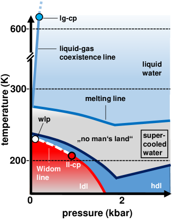
Figure 1: Temperature versus pressure phase diagram of water, lg-cp refers to liquid-gas critical point, wlp is the Widom line point and ll-cp indicates the liquid-liquid critical point, which is the focus of the present work. Picture after Gallo1543 ; Gallo .

The system has $N$ sites and coordination number $c$. Because we assign a cell to each site, particles can move through the free volume. The interaction between sites is $\delta\varepsilon$, the system energy $E\{n_{i}\}$ is

$$E\{n_{i}\}=\frac{cN\varepsilon_{0}}{2}-\delta\varepsilon\sum_{<ij>}n_{i}n_{j},$$ (1)

where $\varepsilon_{0}$ is an arbitrary energy value, the volume is claudio

$$V\{n_{i}\}=v_{0}\sum_{i,j}(n_{i}+n_{j})+\sum_{j}n_{j}\delta v=v_{0}N+\delta v\sum_{\ i=1}^{N}n_{i},$$ (2)

where $(n_{i}+n_{j})=N$, $\{n_{i}\}$ when $K$ particles occupy volume $v_{-}$ and $(N-K)$ particles occupy $v_{+}$. Thus each particle is located in a site, and the volume has two possible values. We associate these two volumes with the low- and high-density phases and thus with two distinct energy scales. These are key in understanding why $\Gamma$ is enhanced near the liquid-liquid critical point. We obtain all the observables related to the system from Eqs. (1) and (2) huang . We carry out an isothermal-isobaric analysis and sum $e^{-E/k_{B}T}$ and $e^{-pV/k_{B}T}$ to the partition function, where $k_{B}$ is the Boltzmann constant and $p$ and $T$ are the pressure and temperature of all possible microstates of the system, respectively.

The resulting partition function $Z=Z(N,p,T)$ has the same mathematical structure as the Ising canonical partition function. Because we have not yet solved the three-dimensional Ising model, we use an approximate mean-field solution claudio to obtain the observables. The mean-field theory can be applied to a wide range of systems, including the Ising model and the van der Waals theory for liquid-gas systems huang . Using it we replace the functional integral $Z=N\int(Dm)e^{-E[m,H]}$ with the maximum value of the integrand, the so-called saddle-point approximation. The parameter $m$ is the order-parameter density, and $Dm$ is the volume element. Because this approximation assumes that the only important configuration near the critical point is the one of uniform density, we expect that, because the density fluctuations in the order parameter are strong in this regime, this study of critical phenomena will exhibit artifacts. However Ref. claudio indicates that consistent results can be obtained in this framework. The equation of state for the system is claudio

$$p(T,v)=\frac{Tk_{B}}{\delta v}\ln\left(\lambda\frac{v_{0}+\delta v-v}{v-v_{0}}\right)+c\frac{\delta\varepsilon}{\delta v}\frac{v-v_{0}}{\delta v},$$ (3)

from which we deduce

$$T(p,v)=\frac{\delta v}{k_{B}f(v)}\left[p-c\frac{\delta\varepsilon}{\delta v^{2}}(v-v_{0})\right].$$ (4)

We use Eq. (3) to determine the critical point coordinates $p_{c}=(v_{c},T_{c})$ huang

$$\left(\frac{\partial p}{\partial v}\right)_{T}=0;\hskip 28.45274pt\left(\frac{\partial^{2}p}{\partial v^{2}}\right)_{T}=0.$$ (5)

Thus

$$\left(\frac{\partial p}{\partial v}\right)_{T}=\frac{c\delta\varepsilon}{\delta v^{2}}-\frac{Tk_{B}}{(v_{0}+\delta v-v)(v-v_{0})},$$ (6)

and

$$\left(\frac{\partial^{2}p}{\partial v^{2}}\right)_{T}=Tk_{B}\left[\frac{2(v_{0}-v)+\delta v}{(v_{0}+\delta v-v)^{2}(v-v_{0})^{2}}\right].$$ (7)

We apply these conditions and the critical point parameters are

$$v_{c}=v_{0}+\frac{1}{2}\delta v;\hskip 22.76228ptT_{c}=\frac{c\delta\varepsilon}{4k_{B}},\hskip 22.76228ptp_{c}=\frac{c}{4}\frac{\delta\varepsilon}{\delta v}(2+\ln\lambda).$$

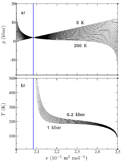
Figure 2: a) Pressure ($p$) versus volume ($V$) phase diagram obtained from Eq. (3) for different values of temperature. The temperature was uniformly varied from 0 to 200 K, with steps of 10 K. The straight line is related to $T=0$ K. Similar results were reported in Ref. [claudio, ]. b) Temperature ($T$) versus volume ($V$) for different values of pressure, which were also varied uniformly as in panel a). The parameters used were the same as in [claudio, ], namely $c=6$, $\delta\varepsilon=1000$ J mol^-1, $v_{0}=(2\times 10^{-5})$ m³ mol^-1, $\delta v=(0.5\times 10^{-5})$ m³ mol^-1 and $\lambda=0.2$.

Employing the basic thermodynamic relations [huang, ] and using $f(v)=\ln\left(\lambda\frac{v_{0}+\delta v-v}{v-v_{0}}\right)$ claudio we obtain the isobaric thermal expansivity $\alpha_{p}$ and the heat capacity $c_{p}$,

$$\alpha_{p}=\frac{1}{v}\left[\frac{\delta v^{2}}{k_{B}f(v)^{2}}g(v)-\frac{c\delta\varepsilon}{k_{B}\delta vf(v)}\right]^{-1},$$ (8)

$$g(v)=\frac{1}{(v_{0}+\delta v-v)(v-v_{0})},$$

and

$$c_{p}=T\frac{k_{B}}{\delta v}f(v)\left[\frac{\delta v^{2}}{k_{B}f(v)^{2}}g(v)-\frac{c\delta\varepsilon}{k_{B}\delta vf(v)}\right]^{-1}.$$ (9)

We use Eqs. (8) and (9) to determine the expression of $\Gamma$ for the system. By definition $\Gamma=\frac{\alpha_{p}}{c_{p}}$ EPJ , and thus using Eqs. (8) and (9) we have

$$\Gamma=\frac{\delta v}{Tk_{B}v}\ln\left(\lambda\frac{v_{0}+\delta v-v}{v-v_{0}}\right).$$ (10)

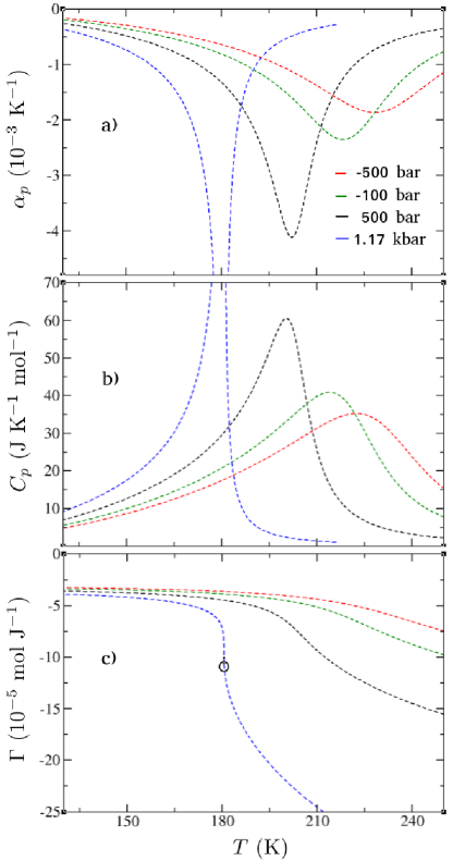
Figure 3: a) Isobaric thermal expansivity $\alpha_{p}$, b) isobaric heat capacity $c_{p}$ and c) Grüneisen parameter $\Gamma$ for different values of pressure. The employed parameters were the same as presented in the caption of Fig. 2. The critical point is indicated by the open circle in c). Further details are discussed in the main text.

We have obtained all the observables and now analyze their behavior near the critical point. Note that because the above equations take the form $c_{p}[T(p,v),]$, $\alpha_{p}(v)$, and $T(p,v)$ they constitute a parametric system. This prevents our obtaining an analytical expression for $v$, and Eq. (3) clearly indicates a transcendental equation in $v$. We thus analyze the behavior of $c_{p}$ and $\alpha_{p}$ by varying $v$, which causes variations in $T$. We fix the critical point parameters by employing the corresponding expressions. We adjust the parameters claudio so that $T_{c}\simeq 180$ K, which is in the No Man’s Land region Gallo .

Figures 2(a) and 2(b) show the $p$–$V$ phase diagram for a range of temperatures and the $T$–$V$ diagram. Note that when $T=0$K the resulting mapping $p(0,v)$ is a straight line. This is obtained using Eq. (3). When the temperature high, the pressure for $v\approx v_{0}$ is higher than when the temperature is low. For $v\approx v_{0}+\delta v$, however, higher temperatures decrease the pressure for fixed values of $v$. Figure 2(b) shows that in a particular range of values of volume, given the pressure values, physical temperature values are inaccessible. Figure 2(a) shows that the point where the pressure is the same for every temperature value (blue vertical line) is the limiting value for the volume $(V)$ for which physical values of the temperature are obtained. Figure 2(b) shows the results using Eq. (3). Note that we cannot analytically obtain expression $v(T,p)$ because Eq. (3) is transcendental in $V$. Thus we have a mapping of these physical quantities [see Eq. (4)], and we can find the corresponding $v$ and $T$ values for each pressure value $(p)$. The same holds for any other desired order of these three parameters. Figures 3(a), 3(b), and 3(c) show the behaviors of $\alpha_{p}$, $c_{p}$, and $\Gamma$, respectively, for different values of pressure. Note that as the pressure is increased, both the minimum of $\alpha_{p}$ and the maximum of $c_{p}$ shift to lower values of temperature, and $\Gamma$ becomes steeper. These features are caused by their proximity to the critical point, which is $p_{c}\approx 1.17$ kbar claudio .

Figure 3(c) shows the effect of pressure on $\Gamma$ and a distinct behavior upon approaching the critical point. Note that the $c_{p}$ and $\alpha_{p}$ features for pressure values near $p_{c}$ are distinct from those observed for $\Gamma$. For $\Gamma$, as $p_{c}$ is approached the variation with temperature reaches a maximum at $T=T_{c}$, indicating the presence of a critical point Barto ; EPJ ; garst ; Cerio . This is our key finding.

The Maxwell-relation $\left(\frac{\partial V}{\partial T}\right)_{p}=-\left(\frac{\partial S}{\partial p}\right)_{T}$ and the negative thermal expansivity shown in Fig. 3 indicate that the entropy of the system is enhanced when approaching the liquid-liquid critical point, i.e., by applying pressure the high- and low-density phases mix and the entropy increases. We also find this in the finite-$T$ critical end-point reported for molecular conductors Barto ; Review-kappa and the quantum critical points in heavy-fermion compounds Zhu ; Kuchler . The high- and low-density phases produce two different energy scales. Because the degree of H-bonding depends on temperature and pressure, a scaling cannot be applied successfully Roland ; Cook . Reference Gallo1543 indicates that water molecule interactions create an open H-bond structure that has a lower density than other configurations. We can capture the energy-scales associated with H-bond configurations that correspond to the low- and high-density phases using a compressible Ising-like model and two accessible system volumes. Using the Landau theory Kadanoff we find that decreasing the order-parameter fluctuations creates divergences in the correlation length Kim1589 and relaxation time Relaxation-time . Reference Casalini reports a connection between the entropy-dependent relaxation time and $\Gamma$. We here suggest that this also is true for supercooled water.

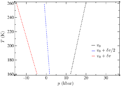
Figure 4: Temperature ($T$) versus pressure ($p$) phase diagram for three different values of volume ($v$), as indicated in the label. A linear relation is observed between $T$ and $p$ for all values of $v$. Moreover, for values near the superior limit of the volume, the pressure reaches negative values and the angular coefficient of the mathematical relation between $T$ and $P$ changes sign. The values of $v_{0}$ and $\delta v$ employed here are the same as in Fig. 2.

We have studied the thermodynamic quantities of a given set of fixed initial parameters. We now extend the model and use it to theoretically predict critical behaviour. Here parameter $\lambda$ is the ratio of characteristic volumes that each particle can occupy, and by changing the $\lambda$ ratio we can use the model to simulate other systems. We thus next analyze $\Gamma$ by varying $\lambda$.

We analyze Eq. 10 and find that varying $\lambda$ changes the critical value of $p_{c}$, but that $T_{c}$ remains the same. This is caused by the non-dependence of $T_{c}$ on $\lambda$. Note that the critical temperature $T_{c}$ depends only on $c$ and $\delta\varepsilon$.

Increasing $\lambda$ increases the critical pressure $p_{c}$. Thus $\Gamma(T)$ increases its temperature values when $\lambda$ is increased. Figure 3(c) shows that $\Gamma$ is sensitive to thermal fluctuations near $T_{c}$. Figure 4 shows that as the pressure is increased for $v=v_{0}+\delta v$, the temperature decreases. We use our compressible Ising-like model to study the Ising-nematic phase recently detected in the low-doping regime of Fe-based superconductors Rafael . An electronic nematic phase is essentially a melted stripe phase Fradkin155 . Figure 4 shows a description of the nematic phase that fixes the model at $v=v_{0}+\delta v$ (red curve). Here the pressure variation is caused by the chemical pressure in the system introduced by the doping effect on the crystal lattice. As the pressure (doping) is varied, the critical point signature vanishes (see Fig. 3). We obtain the same behavior shown in Fig. 4 (red curve) experimentally for the 122 doped Fe-based superconductors budko . In particular, the thermal expansion signatures are suppressed upon doping budko .

Because there are a variety of ways of fitting the parameters, i.e., a variety of constants can be varied, we leave fitting the experimental results reported in Ref. budko to future research. Here we use our model to simulate the doping effect in single crystals by assuming there are two different volumes in the melted electronic nematic phase Fradkin155 . When the system is doped, the electronic nematic phase associated with two coexisting volumes (see the figure in Ref. Fradkin155 ) is suppressed, and the reported superconductivity appears, e.g., for Ba(Fe_1-xCo_x)₂As₂ single crystals budko ; ni .

We have used an energy-volume coupled Ising-like model to calculate the Grüneisen parameter for the liquid-liquid transition in supercooled water claudio . We find that the behavior of the Grüneisen parameter diverges near pressure and temperature values that display anomalously behavior and thus supports the presence of a liquid-liquid critical point governed by two distinct energy scales. In addition to exploring the critical behavior of water and its other phases, our model can also be applied to other systems by adjusting its parameters.

M. de S. acknowledges financial support from the São Paulo Research Foundation – Fapesp (Grants No. 2011/22050-4), National Council of Technological and Scientific Development – CNPq (Grants No. 302498/2017-6), the Austrian Academy of Science ÖAW for the JESH fellowship and Serdar Sariciftci for the hospitality. The Boston University Center for Polymer Studies is supported by NSF Grants PHY-1505000, CMMI-1125290, and CHE-1213217, and by DTRA Grant HDTRA1-14-1-0017.

References

- [1] Pablo G. Debenedett and H. Eugene Stanley, Physics Today 56, 40 (2003).
- [2] Paola Gallo, Katrin Amann-Winkel, Charles Austen Angell, Mikhail Alexeevich Anisimov, Frédéric Caupin, Charusita Chakravarty, Erik Lascaris, Thomas Loerting, Athanassios Zois Panagiotopoulos, John Russo, Jonas Alexander Sellberg, Harry Eugene Stanley, Hajime Tanaka, Carlos Vega, Limei Xu, and Lars Gunnar Moody Pettersson, Chem. Rev. 116, 7463 (2016).
- [3] Peter H. Poole, Francesco Sciortino, Ulrich Essmann, and H. Eugene Stanley, Nature 360, 324 (1992).
- [4] Pradeep Kumar, S. V. Buldyrev, S. R. Becker, P. H. Poole, F. W. Starr, and H. E. Stanley, Proc. Natl. Acad. Sci. U.S.A. 104, 9575 (2007).
- [5] Giancarlo Franzese and H Eugene Stanley, J. Phys.: Condens. Matter 19, 205126 (2007).
- [6] Paola Gallo and H. Eugene Stanley, Science 358, 1543 (2017).
- [7] Kyung Hwan Kim, Alexander Späh, Harshad Pathak, Fivos Perakis, Daniel Mariedahl, Katrin Amann-Winkel, Jonas A. Sellberg, Jae Hyuk Lee, Sangsoo Kim, Jaehyun Park, Ki Hyun Nam, Tetsuo Katayama, and Anders Nilsson, Science 358, 1589 (2017).
- [8] Lorenz Bartosch, Mariano de Souza, and Michael Lang, Phys. Rev. Lett. 104, 245701 (2010).
- [9] Mariano de Souza and Lorenz Bartosch, J. Phys.: Condens. Matter 27, 053203 (2015).
- [10] Mariano de Souza, Paulo Menegasso, Ricardo Paupitz, Antonio Seridonio, and Roberto E Lagos, Eur. J. Phys. 37, 055105 (2016).
- [11] Claudio A. Cerdeiriña and H. Eugene Stanley, Phys. Rev. Lett. 120, 120603 (2018).
- [12] Claudio A. Cerdeiriña, Gerassimos Orkoulas, and Michael E. Fisher, Phys. Rev. Lett. 116, 040601 (2016).
- [13] Claudio A. Cerdeiriña and Gerassimos Orkoulas, Phys. Rev. E 95, 032105 (2017).
- [14] K. Huang, Statistical Mechanics (Wiley, 1987).
- [15] Markus Garst and Achim Rosch, Phys. Rev. B 72, 205129 (2005).
- [16] F. Decremps, L. Belhadi, D. L. Farber, K. T. Moore, F. Occelli, M. Gauthier, A. Polian, D. Antonangeli, C. M. Aracne-Ruddle, and B. Amadon, Phys. Rev. Lett. 106, 065701 (2011).
- [17] Mariano de Souza and Lorenz Bartosch, J. Phys.: Condens. Matter 27, 053203 (2015).
- [18] Lijun Zhu, Markus Garst, Achim Rosch, and Qimiao Si, Phys. Rev. Lett. 91, 066404 (2003).
- [19] R. Küchler, N. Oeschler, P. Gegenwart, T. Cichorek, K. Neumaier, O. Tegus, C. Geibel, J. A. Mydosh, F. Steglich, L. Zhu, and Q. Si, Phys. Rev. Lett. 91, 066405 (2003).
- [20] C. M. Roland, S. Bair, and R. Casalini, J. Chem. Phys. 125, 124508 (2006).
- [21] Richard L. Cook, H. E. King, and Dennis G. Peiffer, Phys. Rev. Lett. 69, 3072 (1992).
- [22] Leo P. Kadanoff, Wolfgang Götze, David Hamblen, Robert Hecht, E. A. S. Lewis, V. V. Palciauskas, M. Rayl, J. Swift, D. Aspnes, and J. Kane, Rev. Mod. Phys. 39, 395 (1967).
- [23] Cecilie Rønne, Per-Olof Åstrand, and Søren R. Keiding, Phys. Rev. Lett. 82, 2888 (1999).
- [24] R. Casalini, U. Mohanty, and C. M. Roland, J. Chem. Phys. 125, 014505 (2006).
- [25] R. M. Fernandes, A. V. Chubukov, and J. Schmalian, Nature Physics 10, 97 (2014).
- [26] Eduardo Fradkin and Steven A. Kivelson, Science 327, 155 (2010).
- [27] S. L. Bud’ko, N. Ni, S. Nandi, G. M. Schmiedeshoff, and P. C. Canfield, Phys. Rev. B 79, 054525 (2009).
- [28] N. Ni, M. E. Tillman, J. Q. Yan, A. Kracher, S. T. Hannahs, S. L. Bud’ko, and P. C. Canfield, Phys. Rev. B 78, 214515 (2008).