Inference of Users Demographic Attributes based on Homophily in Communication Networks

1 Introduction

Over the past decade, mobile phones have become prevalent in all parts of the world, across all demographic backgrounds. Mobile phones are used by men and women across a wide age range in both developed and developing countries. Consequently, they have become one of the most important mechanisms for social interaction within a population, making them an increasingly important source of information to understand human demographics and human behaviour.

In this work we combine two sources of information: communication logs from a major mobile operator in a Latin American country, and information on the demographics of a subset of the users population. This allows us to perform an observational study of mobile phone usage, differentiated by age groups categories [1, 2]. This study is interesting in its own right, since it provides knowledge on the structure and demographics of the mobile phone market in the studied country.

We then tackle the problem of inferring the age group for all users in the network. We present here an exclusively graph-based inference method relying solely on the topological structure of the mobile network, together with a topological analysis of the performance of the algorithm. The equations for our algorithm can be described as a diffusion process with two added properties: (i) memory of its initial state, and (ii) the information is propagated as a probability vector for each node attribute (instead of the value of the attribute itself). Our algorithm can successfully infer different age groups within the network population given known values for a subset of nodes (seed nodes). Most interestingly, we show that by carefully analysing the topological relationships between correctly predicted nodes and the seed nodes, we can characterize particular subsets of nodes for which our inference method has significantly higher accuracy.

2 Data Set

The dataset used in this work consists of anonymized call detail records (CDR) and SMS (short message service) records collected over a three month period. The dataset contains no personal information. We aggregate this information into an edge list $(x,y,w_{x,y})$ where $w_{x,y}$ is a boolean value indicating whether users $x$ and $y$ have communicated at least once within the three month period. This edge list represent our mobile phone graph $\mathcal{G}=\left<\mathcal{N},\mathcal{E}\right>$ where $\mathcal{N}$ denotes the set of nodes (users) and $\mathcal{E}$ the set of communication links. Our graph has about 70 million nodes and 250 million edges. We are also given the age of a subset of 500,000 nodes, which we use as a ground truth (denoted $\mathcal{N}_{GT}$).

3 Age Homophily in the Communication Network

Graph based methods like the one we present in this work rely strongly on the ability of the graph topology to capture correlations between the node attributes we are aiming to predict. A most fundamental structure is that of correlations between a node’s attribute and that of its neighbors. Figure 1(a) shows the correlation matrix ${C}$ where ${C_{i,j}}$ is the number of links between users of age $i$ and age $j$ for the nodes in the ground truth $\mathcal{N}_{GT}$. Though we can observe some smaller off diagonal peaks, we can see that it is most strongly peaked along the diagonal, showing that users are much more likely to communicate with users of their same age.

To account for a population density bias, we compute a surrogate correlation matrix ${R}$ as the expected number of edges between ages $i$ and $j$ under the null hypothesis of independence. This matrix represents a graph with the same nodes as the original, but with random edges (while maintaining the same number of edges as the original). Both ${C}$ and ${R}$ are represented with a logarithmic color scale. If we subtract the logarithm of ${R}$ to the logarithm of the original matrix ${C}$, we can isolate the “social effect” (i.e. homophily) from the pure random connections, as can be seen in Fig. 1(b).

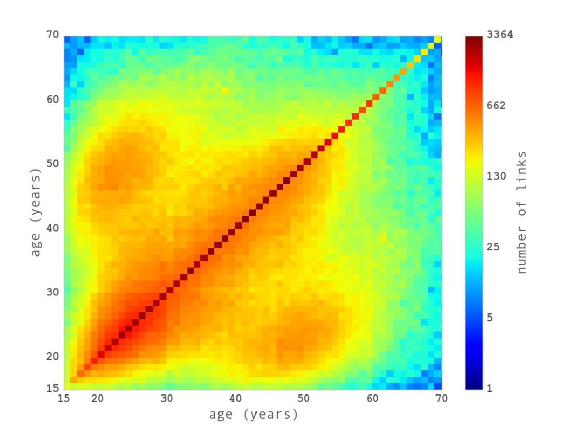
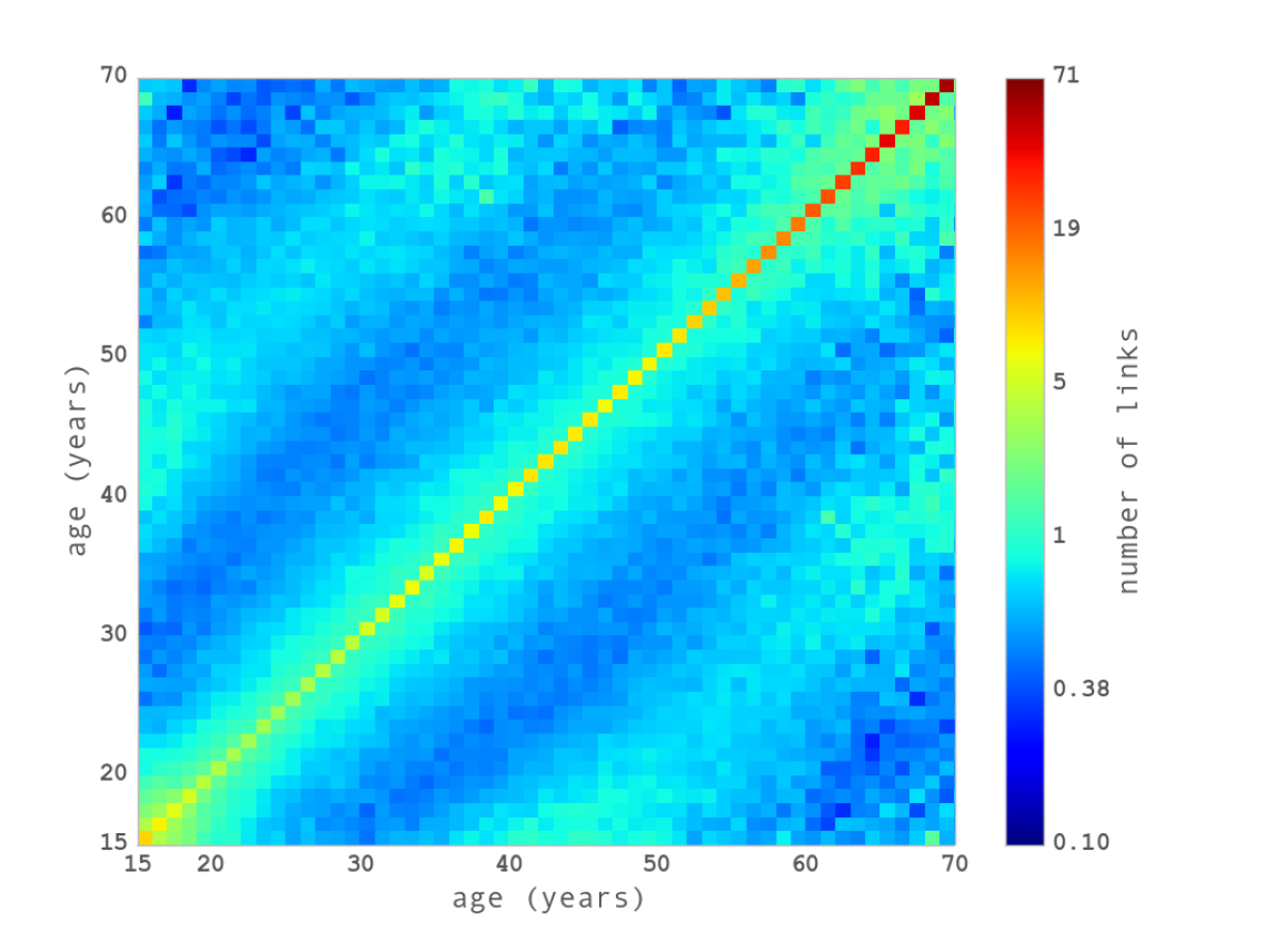
(a) Communications matrix $C$. (b) Difference between $C$ and $R$.

Figure 1: Age homophily plots showing (a) the communications matrix $C$ and (b) the difference between $C$ and the surrogate random links matrix $R$.

4 Reaction-Diffusion Algorithm

For each node $x$ in $\mathcal{G}$ we define an initial state probability vector ${g}_{x,0}\in\mathbb{R}^{4}$ representing the initial probability of the nodes age belonging to one of $d=4$ age categories: below 24, 25 to 34, 35 to 50, and over 50 years old. More precisely, each component of ${g}_{x,0}$ is given by

$$({g}_{x,0})_{i}=\begin{cases}\delta_{i,a(x)}&\text{if }x\in\mathcal{N}_{S}\\ 1/d&\text{if }x\not\in\mathcal{N}_{S}\end{cases}$$ (1)

where $\delta_{i,a(x)}$ is the Kronecker delta function, $a(x)$ the age category assigned to each seed node $x$, and $\mathcal{N}_{S}\subset\mathcal{N}_{GT}$ are the seed nodes, whose known age attribute is diffused across the network. For non-seed nodes, equal probabilities are assigned to each category. These probability vectors are the set of initial conditions for the algorithm.

The evolution equations for the probability vectors ${g}$ are then as follows:

$$\begin{split}{g}_{x,t}=(1-\lambda)\;{g}_{x,0}+\lambda\;\frac{\sum_{x\sim y}{g}_{y,t-1}}{|\{y:x\sim y\}|}\end{split}$$ (2)

where $x\sim y$ is the set of $x$’s neighbours and $\lambda\in[0,1]$ defines the relative importance of each of the two terms. It is not hard to show [1] that the above equation can be rewritten as a discrete reaction diffusion equation on the mobile phone graph given by

$${g}_{t}^{a}-{g}_{t-1}^{a}=(1-\lambda)({g}_{0}^{a}-{g}_{t-1}^{a})-\lambda{\mathcal{L}}{g}_{t-1}^{a}$$ (3)

where $\mathcal{L}$ is a normalized graph Laplacian. At each iteration, each ${g}_{x,t}$ in (2) updates its state as a result of its initial state and the mean field resulting from the probability vector of its neighbors.

Preserving Age Demographics

A salient feature of our algorithm is that the demographic information being spread is not the age group itself, but a probability vector for each age group. In each iteration, the algorithm does not collapse the information in each node to a preferred value; instead it allows the system to evolve as a probability state over the network, which allows us to impose further external constraints on the algorithm’s results. For instance, after the last iteration, we can select the age category of each node based on the final probability state of each node’s category, but constrained so that the age group distribution for the whole network be that of the ground truth set $\mathcal{N}_{GT}$ as was described in [1, 2].

5 Results

In this section we first present the results for the predictive power of the reaction-diffusion algorithm over the whole network $\mathcal{G}$. The overall performance for the entire validation set ($20\%$ of $\mathcal{N}_{GT}$) was $46.6\%$, and we note that a performance based on random guessing without prior information would result in an expected performance of $25\%$, or an expected performance of $\sim 36\%$ if we set all nodes age group to the most probable category ($35-50$). We now take a closer look and see how the performance can increase or decrease as we select particular subsets of nodes.

Topological Metrics and Performance

We first look at how our algorithm performs for different subsets of $\mathcal{N}$ selected according to three topological metrics: (i) number of seeds in the node’s neighborhood, (ii) distance of node to $\mathcal{N}_{S}$ and (iii) node’s degree.

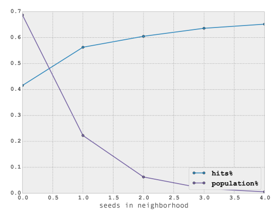
Figure 2: Performance and population as function of SIN (seeds in neighborhood).

Figure 2 plots the performance (hits) of the algorithm as a function of the number of seeds in the node’s neighborhood (SIN). The algorithm performs worse for nodes with no seeds in the immediate neighborhood with hits = 41.5%, steadily rising as the amount of seeds increase with a performance of hits = 66% for nodes with 4 seeds in their neighbourhood. We also see that the population of nodes decreases exponentially with the amount of seeds in their neighbourhood.

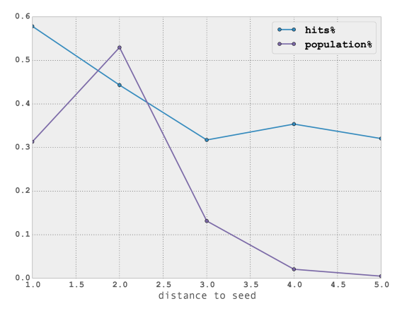
Figure 3: Performance and population as function of DTS (distance to seeds set).

Next we examine how the algorithm performs for nodes in $\mathcal{G}$ that are at a given distance to the seed set (DTS). In Fig. 3 we plot the population size of nodes as a function of their DTS. The most frequent distance to the nearest seed is 2, and almost all nodes are at distance less than 4. This implies that after four iterations of the algorithm, the seeds information have spread to most of the nodes in $\mathcal{G}$. This figure also shows that the performance of the algorithm decreases as the distance of a node to $\mathcal{N}_{S}$ increases.

In Fig. 4 we see that the performance of the algorithm is lowest for nodes with small degree and gradually increases as the degree increases reaching a plateau for nodes with $d(x)>10$.

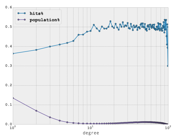
Figure 4: Performance and node population as function of the nodes degree.

Probability Vector Information

An orthogonal approach to find an optimal subset of nodes (where our algorithm works best) is to exploit the information in the probability vector for the age group on each node. Namely, we examine the performance of the reaction-diffusion algorithm as we restrict our analysis to nodes whose selected category satisfies a minimal threshold value $\tau$ in its probability vector.

In Fig. 5 we observe a monotonic increase in the performance as the threshold is increased but, as expected there is a monotonic decrease of the validation set size. We note that for $\tau=0.5$ the performance increased to $72\%$ with 3,492 out of the 143,240 (2.4%) of the validation nodes remaining. The performance of the algorithm increases to $\sim 81\%$ for $\tau=0.55$ but the validation set remaining sharply decreased to only 201 nodes ($0.1\%$).

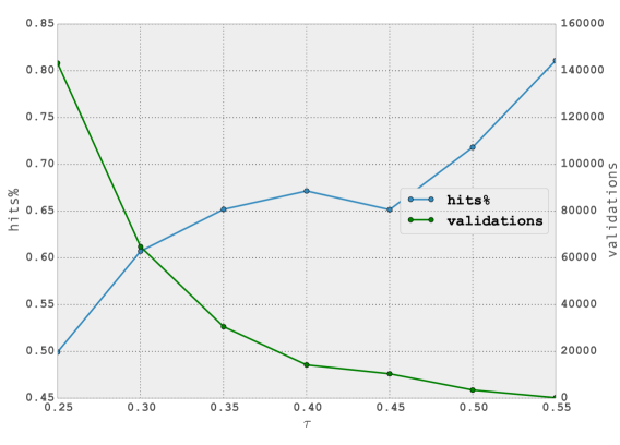
Figure 5: Performance as function of $\tau$.

6 Conclusions

In this work we have presented a novel algorithm that can harness the bare bones topology of mobile phone networks to infer with significant accuracy the age group of the network’s users. We show that an important reason for the success of the algorithm is the strong age homophily among neighbours in the network as evidenced by our observational study of the ground truth sample $\mathcal{G}_{GT}$.

We have shown the importance of understanding nodes topological properties, in particular their relation to the seed nodes, in order to fine grain our expectation of correctly classifying the nodes. Though we have carried out this analysis for a specific network, we believe this approach can be useful to study generic networks where node attribute correlations are present.

As future work, one direction that we are investigating is how to improve the graph based inference approach presented here by appropriately combining it with classical machine learning techniques based on node features [2]. We are also interested in applying our methodology to predict variables related to the users’ spending behavior. In [3] the authors show correlations between social features and spending behavior for a small population. We are currently tackling the problem of predicting spending behavior characteristics on the scale of millions of individuals.

References

- [1] J. Brea, J. Burroni, M. Minnoni, and C. Sarraute. Harnessing mobile phone social network topology to infer users demographic attributes. In Proceedings of the 8th Workshop on Social Network Mining and Analysis (SNA KDD). ACM, 2014.
- [2] C. Sarraute, P. Blanc, and J. Burroni. A study of age and gender seen through mobile phone usage patterns in Mexico. In 2014 IEEE/ACM International Conference on Advances in Social Networks Analysis and Mining. ACM, 2014.
- [3] V. K. Singh, L. Freeman, B. Lepri, and A. S. Pentland. Predicting spending behavior using socio-mobile features. In Social Computing (SocialCom), 2013 International Conference on, pages 174–179. IEEE, 2013.