Color matrix element corrections for parton showers

Abstract

We investigate the effects of keeping the full color structure for parton emissions in parton showers for both LEP and LHC. This is done within the Herwig 7 dipole shower, and includes gluon emission, gluon splitting, initial state branching processes, as well as hadronization. The subleading $N_{c}$ terms are included as color matrix element corrections to the splitting kernels by evolving an amplitude-level density operator and correcting the radiation pattern for each parton multiplicity, up to a fixed number of full color emissions, after which a standard leading color shower takes over. Our results are compared to data for a wide range of LEP and LHC observables and show that the subleading $N_{c}$ corrections tend to be small for most observables probing hard, perturbative dynamics, for both LEP and LHC. However, for some of these observables they exceed 10%. On soft physics we find signs of significantly larger effects.

1 Introduction

At present time event generators Sjostrand:2007gs ; Bahr:2008pv ; Bellm:2015jjp ; Gleisberg:2003xi have developed into indispensable tools for understanding collider phenomenology. At the same time, the high energy available at the LHC has significantly opened up the perturbative phase space available for radiation. This increases the demand of resummation, performed either analytically or, as in the case of parton showers, numerically e.g. via the Sudakov veto algorithm Platzer:2011dq ; Platzer:2011dr .

From a QCD perspective, the high number of colored partons due to the large perturbative phase space, as well as due to the fact that the initial state partons carry color, calls for a better understanding of subleading $N_{c}$ effects.

This is also in demand to ease the cancellation of infrared singularities in the matching and merging of parton showers with NLO calculations Platzer:2011bc ; Platzer:2012bs ; Bellm:2017ktr , which often fully include subleading $N_{c}$ effects. It should also be stressed that we expect such corrections to account for subleading $N_{c}$, leading-logarithmic problems which can arise in dipole-type parton shower algorithms due to an ambiguous definition of an emitter’s color charge Dasgupta:2018nvj .

To achieve greater accuracy and better understanding of parton shower uncertainties, it is therefore time to include a better description of subleading color contributions in parton showers, similar to how parton showers recently have been improved by matrix element merging at leading order Lonnblad:2001iq ; Krauss:2002up ; Hoche:2006ph ; Lavesson:2007uu ; Hoeche:2009rj ; Hamilton:2009ne , and matching at next-to-leading order Dobbs:2001dq ; Frixione:2002ik ; Nason:2004rx ; Nagy:2005aa ; Frixione:2010ra ; Platzer:2011bc .

The first steps in this direction has already been performed by some of the authors in the case of an $e^{+}e^{-}$-collider Platzer:2012np . Others have pursued another road, keeping only a subset of the color suppressed terms Nagy:2012bt ; Nagy:2015hwa , and detailed studies have been carried out towards systematically expanding virtual and real effects in shower-type evolution algorithms Platzer:2013fha ; Martinez:2018ffw .

In the present paper we extend the color matrix element corrections, first implemented in Platzer:2012np , by including initial state hadrons as well as $g\rightarrow q\overline{q}$-splittings, subsequent leading color showering and hadronization. This is done within the Herwig 7.1 Bellm:2017bvx implementation of the dipole shower algorithm Platzer:2009jq , giving us a full-fledged general purpose event generator which can be used for studying color matrix element corrections to any process occurring at the LHC and other colliders, in practice up to a limited number of colored partons, restricted by the fast growing complexity in color space, however still reaching down to relatively soft emissions.

Our method is based on dipole factorization Catani:1996jh ; Catani:1996vz , which we outline in section 2. The complication brought about by the color matrix element corrections is discussed in section 3, and implementation details, involving evolution of the color structure treatment, the weighted Sudakov algorithm and the density operator, are discussed in section 4, 5 and 6 respectively. Results for various processes, including initial and final state radiation, standard QCD observables, heavy quark production and $Z$ plus jets are discussed in section 7, and concluding remarks are made in section 8.

2 Essence of dipole factorization and dipole shower evolution

This paper is based on dipole factorization, stating that whenever the next gluon to be emitted from an $n$-parton configuration becomes either soft or collinear to one of the existing partons, the squared amplitude for the $n+1$-parton case can be approximated with

$$|{\cal M}_{n+1}(...,p_{i},...,p_{j},...,p_{k},...)|^{2}\approx\\ \sum_{k\neq i,j}\frac{1}{2p_{i}\cdot p_{j}}\langle{\cal M}_{n}(...,p_{\tilde{ij}},...,p_{\tilde{k}},...)|{\mathbf{V}}_{ij,k}(p_{i},p_{j},p_{k})|{\cal M}_{n}(...,p_{\tilde{ij}},...,p_{\tilde{k}},...)\rangle\ ,$$ (1)

in terms of the old amplitude $|{\cal M}_{n}\rangle$. In the above, an emitter $\tilde{ij}\rightarrow i,j$ whereas a spectator $k\rightarrow\tilde{k}$ absorbs the longitudinal recoil, such that all partons, before and after emission, stay on-shell. For final state radiation we use the standard Sudakov decomposition,

$$p_{i} = zp_{\tilde{ij}}+\frac{p_{\perp}^{2}}{zs_{ijk}}p_{\tilde{k}}+k_{\perp}$$ (2)

$$p_{j} = (1-z)p_{\tilde{ij}}+\frac{p_{\perp}^{2}}{(1-z)s_{ijk}}p_{\tilde{k}}-k_{\perp}$$ (3)

$$p_{k} = \left(1-\frac{p_{\perp}^{2}}{z(1-z)s_{ijk}}\right)p_{\tilde{k}}\;,$$ (4)

with $p_{\tilde{ij}}^{2}=p_{\tilde{k}}^{2}=0$, a spacelike transverse momentum $k_{\perp}$ with $k_{\perp}^{2}=-p_{\perp}^{2}$ and $k_{\perp}\cdot p_{\tilde{ij}}=k_{\perp}\cdot p_{\tilde{k}}=0$. The cases of initial state emitter or spectator are discussed in Platzer:2009jq .

Note that the sum in eq. (1) only runs over $\tilde{ij}\neq\tilde{k}$. This is possible since the collinear singularity corresponding to the square of the diagram where parton $\tilde{ij}$ is the emitter, has been rewritten as a sum of interferences between that diagram and every other diagram using color conservation

$${\mathbf{T}}_{\tilde{ij}}^{2}=-\sum_{k\neq\tilde{ij}}{\mathbf{T}}_{\tilde{ij}}\cdot{\mathbf{T}}_{k}\ .$$ (5)

The splitting kernels are given in terms of the standard dipole splitting kernels as

$${\mathbf{V}}_{ij,k}(p_{i},p_{j},p_{k})=-8\pi\alpha_{s}V_{ij,k}(p_{i},p_{j},p_{k})\frac{{\mathbf{T}}_{\tilde{ij}}\cdot{\mathbf{T}}_{k}}{{\mathbf{T}}_{\tilde{ij}}^{2}}\ ,$$ (6)

where ${\mathbf{T}}_{\tilde{ij}}\cdot{\mathbf{T}}_{k}$ describes the color space effect of exchanging a gluon between parton $\tilde{ij}$ and parton $\tilde{k}$, and thus contains an implicit sum over gluon indices. In the massless case, the final-final dipole splitting kernels are given by

$$V_{qg,k}(p_{i},p_{j},p_{k}) = C_{F}\left(\frac{2(1-z)}{(1-z)^{2}+p_{\perp}^{2}/s_{ijk}}-(1+z)\right)$$

$$V_{gg,k}(p_{i},p_{j},p_{k}) = 2C_{A}\left(\frac{1-z}{(1-z)^{2}+p_{\perp}^{2}/s_{ijk}}+\frac{z}{z^{2}+p_{\perp}^{2}/s_{ijk}}-2+z(1-z)\right)\ .$$ (7)

Note, however, that dipole factorization is valid also for massive particles in the quasi-collinear limit, and our implementation is general, using the massive dipole splitting kernels and kinematics available in Herwig, as detailed in ttbarPaper . For the dipole configurations involving initial state partons, we use the corresponding expressions as given in Catani:1996vz ; Catani:2002hc . In eq. (7) the factors of $C_{F}=T_{R}(N_{c}^{2}-1)/N_{c}$ and $C_{A}=2T_{R}N_{c}$, where $T_{R}$ is defined by $\operatorname*{\mathrm{tr}}(t^{a}t^{b})=T_{R}\delta^{ab}$, explains the inclusion of ${\mathbf{T}}_{\tilde{ij}}^{2}$ in eq. (6); in order to use the standard definition of eq. (7), ${\mathbf{T}}_{\tilde{ij}}^{2}$ is introduced in the denominator of eq. (6).

In the large $N_{c}$ limit the color correlator becomes

$$-\frac{{\mathbf{T}}_{\tilde{ij}}\cdot{\mathbf{T}}_{k}}{{\mathbf{T}}_{\tilde{ij}}^{2}}\rightarrow\frac{1}{1+\delta_{\tilde{ij}}}\delta(\tilde{ij},k\text{ color connected})\ ,$$ (8)

where $\delta_{\tilde{ij}}\equiv 1$ if $\tilde{ij}$ is a gluon, and zero otherwise. In this way, the factor $C_{F}$ for gluon emission off a quark is reproduced in the large $N_{c}$ limit by coherent emission from the quark and its color-connected partner, and the factor $C_{A}$ is reproduced for gluon splitting by the sum of the coherent emissions from the gluon and its two color-connected partners, hence the factor $1/2$ for gluons in eq. (8).

We remark that the leading $N_{c}$ version of the above describes how to get a leading $N_{c}$ correct emission pattern. It does not address the issue of assigning a leading $N_{c}$ color flow from which subsequent emission can be performed. The default strategy is to use a color flow where the radiated gluon is inserted between the emitter and the spectator. However, with a gluon splitting kernel which is symmetric in $z\leftrightarrow 1-z$, the question of which gluon is the radiator and which is radiated arises. In the limit where $z$ is small, it is rather the parton with momentum fraction $z$ which is soft and thus should be seen as radiated and therefore be inserted between the emitter (with the large momentum fraction $1-z$) and the spectator. For this reason, to mimic the swap of color, we swap momenta of the emitter and the emitted parton with probability $1-z$, such that the soft gluon always tends to be inserted between the harder parton and the spectator in the color structure, guaranteeing that we get the correct soft limit. We remark, however that the probability $1-z$ is a choice, and that and any function, having the same limits when $z\rightarrow 1$ and $z\rightarrow 0$, would have been a valid choice. Alternatively, the splitting kernels could have been redefined to only contain the $1-z$ singularity (see Gustafson:1987rq ; Bellm:2018wwz for comparison).

As we want to describe LHC collisions, the color matrix element corrections have to be applied also to initial state hadrons, meaning that we have to deal with initial-initial emissions as well as initial-final and final-initial emissions. The initial state emission cases are treated in a standard backward evolution scheme, meaning that if the emitter is an initial state parton, the backward evolution is done by folding in the parton distribution functions (PDFs), using appropriate splitting kernels, and colors are updated as if the resulting (low energy) parton was emitted. To be more precise, denoting the emitter participating in the hard process by $i$, the radiated parton with $j$, and the (initial) parton going into the PDF by $\tilde{ij}$, the used splitting kernel is $P_{\tilde{ij}\rightarrow ij}$, and the emission probability is evolved using PDF ratios Sjostrand:1985xi , as described in section 6.5 in Bahr:2008pv . The color structure of the full color shower, on the other hand, is, as discussed in section 6, treated as if $i\rightarrow\tilde{ij},j$.

In the shower algorithm presented here, we also extend our analysis from Platzer:2012np by including $g\rightarrow q\overline{q}$ splitting. The description of how this splitting fits into the dipole formalism is given in section 6.

3 Color matrix element corrections

We like to stress that this paper deals with color matrix element corrections to parton showers. We thus correct each emission with the full color correlations, keeping all soft and collinear contributions to the emission, i.e., we use the right "antenna pattern". In this sense, we do more than the standard leading $N_{c}$ showers — where only the leading $N_{c}$-terms, and the color suppressed term in $C_{F}=T_{R}(N_{c}^{2}-1)/N_{c}$, are kept — but less than a full matrix element correction.

We thus start from some color amplitude, $|{\cal M}_{n}\rangle$, for $n$ colored partons, decomposed in any arbitrary color basis, with basis vectors $|\alpha_{n}\rangle$

$$|{\cal M}_{n}\rangle=\sum_{\alpha=1}^{d_{n}}c_{n,\alpha}|\alpha_{n}\rangle\quad\leftrightarrow\quad{\cal M}_{n}=(c_{n,1},...,c_{n,d_{n}})^{T}\ .$$ (9)

Squaring the amplitude in order to calculate a cross section gives

$$|{\cal M}_{n}|^{2}={\cal M}_{n}^{\dagger}S_{n}{\cal M}_{n}=\mathop{\rm Tr}\left(S_{n}\times{\cal M}_{n}{\cal M}_{n}^{\dagger}\right)$$ (10)

with $S_{n}$ being the scalar product matrix, $(S_{n})_{\alpha\beta}=\langle\alpha_{n}|\beta_{n}\rangle$, for color basis vectors $|\alpha_{n}\rangle$ and $|\beta_{n}\rangle$. Upon emission from the $\tilde{ij},\tilde{k}$-pair, the relevant color factor changes to

$$\langle{\cal M}_{n}|{\mathbf{T}}_{\tilde{ij}}\cdot{\mathbf{T}}_{\tilde{k}}|{\cal M}_{n}\rangle=\mathop{\rm Tr}\left(S_{n+1}\times T_{\tilde{k},n}{\cal M}_{n}{\cal M}_{n}^{\dagger}T_{\tilde{ij},n}^{\dagger}\right)$$ (11)

in terms of matrix representations, ${T}_{\tilde{ij}},{T}_{\tilde{k}}\in{\mathbb{C}}^{d_{n+1},d_{n}}$, of ${\mathbf{T}}_{\tilde{ij}},{\mathbf{T}}_{\tilde{k}}$.

While this improves the radiation pattern to fixed order, we should remark that it is not the full story of color suppressed terms in the context of parton showers. To fully include all subleading $N_{c}$ terms in the soft and collinear limits, virtual color rearranging terms associated with the same singularity structure should also be kept. To accomplish this, a full resummation of virtual exchanges is needed. Unfortunately, within the current event generator structure these contributions cannot be included, and we postpone their inclusion for future work. Instead we present a fully functional subleading $N_{c}$ dipole shower, building on the algorithm presented in Platzer:2012np , but including $g\rightarrow q\overline{q}$ splitting, hadronization, full mass dependence and initial state hadrons, meaning final-final, initial-final, final-initial and initial-initial dipoles.

The rewriting of the collinear singularities in terms of dipole splitting kernels eqs. (6-7), using color conservation, eq. (5), means that the color flow will be replaced by every other color flow, except the flow associated with the color structure of the collinear singularity. In order to be able to continue the full $N_{c}$ matrix element corrected parton shower with a leading $N_{c}$ parton shower (as well as with subsequent hadronization), we do, however, keep the color structure associated with emission from the emitter, as in the standard event record, and we use that for the subsequent leading $N_{c}$ shower and hadronization. Not having one color structure to start from when it comes to hadronization would imply considering a new approach to a hadronization model, which is much beyond the scope of the current paper. On the other hand, it is still interesting to add hadronization in a standard way to enable comparison to data.

4 Color structure treatment

So far, the treatment of color structure in this paper has been completely basis independent. Any complete spanning set of relevant color structures, such as trace bases Paton:1969je ; Berends:1987cv ; Mangano:1987xk ; Mangano:1988kk ; Kosower:1988kh ; Nagy:2007ty ; Sjodahl:2009wx ; Alwall:2011uj ; Sjodahl:2014opa ; Platzer:2012np , multiplet bases Kyrieleis:2005dt ; Dokshitzer:2005ig ; Sjodahl:2008fz ; Beneke:2009rj ; Keppeler:2012ih ; Du:2015apa ; Sjodahl:2015qoa , or color flow bases 'tHooft:1973jz ; Kanaki:2000ms ; Maltoni:2002mq would do, as long as the matrices $T_{\tilde{ij},n}$ for gluon emission, the matrices $t_{\tilde{ij},n}$ describing gluon splitting and the scalar product matrices $S_{n}$ could be calculated. This basis freedom is maintained within the Matchbox module of Herwig, which can be used to interface to any implementation of color structure, such as CVolver Platzer:2013fha or ColorFull Sjodahl:2014opa .

For our simulations we use trace bases and the ColorFull implementation Sjodahl:2014opa . In the trace bases, the color structure is expressed in terms of open and closed quark-lines, of the form

(12)

for all possible quark and gluon permutations and all possible number of traces Sjodahl:2009wx ; Sjodahl:2014opa . These bases have several advantages. The color structure can trivially be translated into the leading $N_{c}$ color flow, which is needed for subsequent leading $N_{c}$ emission and standard hadronization. The processes of gluon emission, gluon splitting, and gluon exchange can all be very easily described, giving respectively at most two, two and four new basis vectors Mangano:1988kk ; Nagy:2007ty ; Sjodahl:2009wx . For example, considering gluon emission off an open quark-line we have the two trace basis vectors

$$\parbox{113.81102pt}{\includegraphics[width=113.81102pt]{Figures/GluonEmission1.pdf}}=\parbox{113.81102pt}{\includegraphics[width=113.81102pt]{Figures/GluonEmission2ColorLines.pdf}}-\parbox{113.81102pt}{\includegraphics[width=113.81102pt]{Figures/GluonEmission3ColorLines.pdf}}\ ,$$ (13)

where we have also illustrated the different color flows in the $N_{c}\rightarrow\infty$ limit. If we instead consider gluon splitting, we have

$$\parbox{113.81102pt}{\includegraphics[width=113.81102pt]{Figures/GluonSplitting1.pdf}}=T_{R}\left[\parbox{113.81102pt}{\includegraphics[width=113.81102pt]{Figures/GluonSplitting2ColorLines.pdf}}-\frac{1}{N_{c}}\parbox{113.81102pt}{\includegraphics[width=113.81102pt]{Figures/GluonSplitting3ColorLines.pdf}}\right]\ .$$ (14)

One of the disadvantages of trace basis lies in their overcompleteness, meaning that hence — strictly speaking — they are actually not bases, but rather spanning sets.

For a small set of partons, up to approximately five $q\overline{q}$-pairs and gluons, the overcompleteness is fairly moderate, but for more partons it becomes significant Keppeler:2012ih ; Sjodahl:2015qoa . The number of basis vectors scales as a factorial in the trace basis case, with roughly $(N_{g}+N_{q\overline{q}})!/e$ basis vectors Keppeler:2012ih , whereas the number of basis vectors for finite $N_{c}$ scale only as an exponential. On the other hand, basis vectors which are not needed for a given process can often easily be identified and crossed out for trace bases, in particular, at tree-level, the number of required basis vectors scales approximately as $(N_{g}+N_{q\overline{q}}-1)!$. For example, in eq. (12), only color structures where all gluons are attached to the open quark-lines contribute.

The overcompleteness, and the fact that the scalar product matrices are dense, i.e., the scalar product between most pairs of basis vectors does not vanish, is the Achilles’ heel of the trace bases. Instead of vanishing for two different basis vectors, the scalar product is suppressed by one or more powers of $1/N_{c}$. Thus, when $N_{c}\rightarrow\infty$, the bases are orthogonal, and the color structure can be replaced by color flows, as in eq. (13) and eq. (14). Since we keep the full color structure, it is the calculation of scalar products that limits the number of subleading $N_{c}$ emissions that we can keep. At about $N_{g}+N_{q\overline{q}}=6$, the color structure calculations start to take up significant time, and going beyond $N_{g}+N_{q\overline{q}}=7$ is very time consuming within our current setup.

This unfavorable scaling behavior could be circumvented by using orthogonal multiplet bases Keppeler:2012ih ; Sjodahl:2015qoa , in which case the calculation of the radiation matrices $T_{\tilde{ij},n}$ would be more time consuming, however not to the same degree Du:2015apa . Alternatively color structure could be sampled over. This is a road which we have attempted to pursue. Within our current framework, using the weighted Sudakov veto algorithm from Bellm:2016voq (modified as described in section 5), it is, however, impractical to go beyond 3 subleading $N_{c}$ emissions at LEP, or two subleading $N_{c}$ emissions at LHC, due to the very poor statistical convergence from large weight fluctuations. Therefore, within our current implementation, sampling has proven disadvantageous.

5 The weighted Sudakov algorithm

The shower described in this paper treats up to $N_{\mathrm{max}}$ emissions with the full color correlations. This corrects the emissions to appear first in the $p_{\perp}$-ordered evolution, down to smaller scales, and then the leading color shower handles the subsequent lower $p_{\perp}$ emissions. The radiation pattern we aim at describing in the full color shower is

$${\rm d}P_{ij,k}(p_{\perp}^{2},z;p_{\tilde{ij}},p_{\tilde{k}})=\frac{\alpha_{s}}{2\pi}\frac{{\rm d}p_{\perp}^{2}}{p_{\perp}^{2}}{\rm d}z{\cal J}(p_{\perp}^{2},z;p_{\tilde{ij}},p_{\tilde{k}})V_{ij,k}(p_{\perp}^{2},z;p_{\tilde{ij}},p_{\tilde{k}})\times\frac{-1}{{\mathbf{T}}_{\tilde{ij}}^{2}}\frac{\langle{\cal M}_{n}|{\mathbf{T}}_{\tilde{ij}}\cdot{\mathbf{T}}_{\tilde{k}}|{\cal M}_{n}\rangle}{|{\cal M}_{n}|^{2}},$$ (15)

where the factor after the multiplication sign is the color matrix element correction, which we will denote by $\omega_{\tilde{ij}\,\tilde{k}}^{n}$. For the cases when the color matrix element correction is negative, the weighted Sudakov veto algorithm from Bellm:2016voq is used, with one modification: In the competition version of the algorithm from Bellm:2016voq , the weight for an emission gets a contribution from each veto and accept step, for all trial emissions of all competing pairs. The algorithm will, however, produce the same distribution if the total weight only receives contributions from the accept step of the winning emission and veto steps at scales larger than the winning scale. Discarding all weight contributions below some scale (in this case the scale of the winning emission) makes the algorithm generate another distribution below that scale, but the radiation pattern of the losing trial emissions below the winning scale cannot affect the final distribution, since these emissions are discarded anyway. However, the convergence of the algorithm gets worse, due to large weight fluctuations. We therefore choose to discard the weights below the winning scale. This modification significantly improves the convergence.

Two choices in the algorithm from Bellm:2016voq are: the acceptance probability (denoted $\epsilon$ in Bellm:2016voq ) and the overestimate proposal distribution (denoted $R$). These free choices were used to improve the convergence of the algorithm, the details of the choices can be found in appendix A.

In total, to reproduce the radiation pattern in eq. (15), the shower steps given below are repeated until $N_{\mathrm{max}}$ emissions have been corrected or no emission is found above the cut-off scale $\mu$.

1. The starting scale $Q_{\perp}$ is given by the hard scale. For the first emission, this is taken to be the $Z$ mass for LEP and the average transverse momentum of hard jets in the final state for LHC. For subsequent emissions, $Q_{\perp}$ is given by the scale of the previous emission.

2. All processes for all pairs of partons compete with each other and a winning hardest scale is chosen. For each dipole, $\tilde{ij},\tilde{k}$, candidate emissions, $\tilde{ij},\tilde{k}\rightarrow i,j,k$ at scales $p_{\perp,\tilde{ij},k}$, are chosen according to the Sudakov form factor

   $$-\ln\Delta_{ij,k}(p_{\perp,ij,k}^{2}|Q_{\perp}^{2})=\frac{\alpha_{s}}{2\pi}\int_{p_{\perp,ij,k}^{2}}^{Q_{\perp}^{2}}\frac{{\rm d}q_{\perp}^{2}}{q_{\perp}^{2}}\int_{z_{-}(q_{\perp}^{2})}^{z_{+}(q_{\perp}^{2})}{\rm d}z\ {\cal P}_{ij,k}(q_{\perp}^{2},z;p_{\tilde{ij}},p_{\tilde{k}})\ ,$$ (16)

   where ${\cal P}_{ij,k}$, in accordance with eq. (15), is

   $${\cal P}_{ij,k}(p_{\perp}^{2},z;p_{\tilde{ij}},p_{\tilde{k}})={\cal J}(p_{\perp}^{2},z;p_{\tilde{ij}},p_{\tilde{k}})V_{ij,k}(p_{\perp}^{2},z;p_{\tilde{ij}},p_{\tilde{k}})\times\frac{-1}{{\mathbf{T}}_{\tilde{ij}}^{2}}\frac{\langle{\cal M}_{n}|{\mathbf{T}}_{\tilde{ij}}\cdot{\mathbf{T}}_{k}|{\cal M}_{n}\rangle}{|{\cal M}_{n}|^{2}}$$ (17)

   and $z_{\pm}(p_{\perp}^{2})$ follow from the phase space boundaries at fixed transverse momentum. If the color matrix element correction is positive, the standard Sudakov veto algorithm is used (resulting in that the trial emission always contributes a factor $1$ to the event weight) and if it is negative, the modified weighted veto algorithm is used (where the weight is, in general, multiplied by the weight in eq. (29)). The winning emission defines the details of the kinematics and the recoil is absorbed by the spectator $\tilde{k}$ of the winning dipole, such that all partons are on-shell after the emission.

3. If no scale above the cut-off $\mu$ was found, the shower terminates.

4. If this is the emission $N_{\mathrm{max}}$, the leading $N_{c}$ shower will continue showering the event, otherwise the density operator is updated as will be described in section 6.

If $N_{\mathrm{max}}$ emissions have been corrected, the leading $N_{c}$ shower continues with the color structure given by the large $N_{c}$ flow associated with emissions from the selected emitters, as discussed in section 3. The leading $N_{c}$ shower then continues until reaching the cut-off scale $\mu$. Finally, the event may, or may not, be hadronized. If the hadronization is performed it starts from the leading $N_{c}$ color flow.

6 Evolution of the density operator

The parton shower starts from the hard matrix element $|{\cal M}_{n}\rangle$. However, after emission, the resulting “dipole” color structure from eq. (11) cannot, within our framework, be cast into the form of some new amplitude $|{\cal M}_{n+1}\rangle$. Instead we see from eq. (11) that the relevant $n+1$-parton quantity, corresponding to $M_{n}\equiv{\cal M}_{n}{\cal M}_{n}^{\dagger}$ for emission from $\tilde{ij},\tilde{k}$ is $\sim T_{\tilde{k},n}{\cal M}_{n}{\cal M}_{n}^{\dagger}T_{\tilde{ij},n}^{\dagger}$. For gluon emission (final or initial), keeping all contributions to the emission probability, and using the dipole factorization eq. (1) with the splitting kernels eq. (6), we see that if we define

$$M_{n+1}=-\sum_{i\neq j}\sum_{k\neq i,j}\frac{4\pi\alpha_{s}}{p_{i}\cdot p_{j}}\frac{V_{ij,k}(p_{i},p_{j},p_{k})}{{\mathbf{T}}_{\tilde{ij}}^{2}}\ T_{\tilde{k},n}M_{n}T_{\tilde{ij},n}^{\dagger}\ ,$$ (18)

the matrix element square for $n+1$ particles can be written analogously to eq. (10) as

$$|{\cal M}_{n+1}|^{2}=\mathop{\rm Tr}\left(S_{n+1}\times M_{n+1}\right).$$ (19)

Thus, when a phase space point has been selected for gluon emission, $M_{n}$ could be updated according to eq. (18). Note, however, that the overall normalization of $M_{n+1}$ is irrelevant, since when used in the $n+2$-version of eq. (17) to calculate the emission of $n+2$ partons, $M_{n+1}$ enters in both the numerator and denominator. Thus we could ignore any constant factor. In fact, for technical reasons, we only keep the eikonal parts, $\sim p_{i}\cdot p_{k}/(p_{i}\cdot p_{j}\,p_{k}\cdot p_{j})$, of eq. (18). Clearly the dropped hard collinear pieces should not alter the subsequent emission of soft wide-angle radiation.

For the case of $g\rightarrow q\overline{q}$, there is no interference between various possible emitters, and the amplitude is symmetric in all final state gluons, meaning that $M_{n}$ can be updated using only one term

$$M_{n+1}=t_{\tilde{ij},n}M_{n}t_{\tilde{ij},n}^{\dagger}\ ,$$ (20)

where $t_{\tilde{ij},n}$ represents the color space map corresponding to $t^{g}_{q\overline{q}}$, i.e., the matrix where element $\alpha\beta$ is the transition from basis vector $\beta$ in the initial (smaller) basis, to basis vector $\alpha$ in the final (larger) basis, where the difference between the color structures is that the gluon $\tilde{ij}$ has been contracted and replaced by the $q\overline{q}$-pair $i,j$, giving one or two new basis vectors. The possible recoil partners used to set up the gluon splitting into quarks are picked using eq. (15) with the $g\rightarrow q\overline{q}$ splitting kernel, but with color matrix element corrections as for gluon emission. While this choice is ad-hoc in this case, it has the advantage of nicely fitting into the dipole picture. In the collinear limit, where the splitting becomes relevant, we can use color conservation eq. (5), to observe that the sum over the kernels using different spectators is indeed collapsing to the expected collinear splitting function.

Note that the same update of $M_{n+1}$, eq. (20), and the same recoil strategy, is applied irrespectively of if the splitting gluon is final or initial. The only difference is thus, as for the gluon emission case, the standard convolution with the PDFs for initial parton splitting rates. If we have an initial state quark (antiquark) which evolves backwards into a gluon going into the parton distribution function and an antiquark (quark) which is radiated, the shower has no interference with other diagrams, and the density matrix can be updated according to

$$M_{n+1}=T_{\tilde{ij},n}M_{n}T_{\tilde{ij},n}^{\dagger}\ ,$$ (21)

without an irrelevant, overall factor. In the standard dipole large $N_{c}$ shower, the momentum recoil is absorbed by the color-connected partner, implying that the emission can be accounted for within the dipole shower formalism.

A comment on the update of the density matrix is in order here. In this paper we keep the full color structure, of all possible emitter-spectator pairs which could have contributed to an emission. An alternative strategy is to pairwise sample over emitters and spectators, corresponding to keeping only one term in the double sum in eq. (18). While this samples from all color structures, we like to remark that it actually corresponds to a slightly different approximation. In our current implementation, after defining the kinematics of the new emission from the winning pair, all pairs contribute to the color structure of the next emission, and the weight of their color structure, is given by eq. (18), implicitly multiplying the same Sudakov factor, the Sudakov factor of the winning pair. In a sampling procedure, the terms in the eq. (18) would end up in different events, and each term would be associated with the Sudakov factor of the pair emitting in that winning phase space point. The difference in a sufficiently large Monte Carlo sample, thus lies within the Sudakov factor, coming with different scales for different pairs. We note however, that the two approaches should agree in the soft limit, and we have also checked that the numerical difference is small.

7 Results

7.1 Outline of the simulation

In this section we outline the simulation, and consider various shower distributions with the aim of understanding and validating the shower evolution.

We use the Herwig 7.1 dipole shower, with settings according to the 7.1.3 release Bellm:2017bvx , with the modified weighted Sudakov veto algorithm outlined in section 5, and with color matrix element corrections as described in section 3, starting from lowest order $2\rightarrow 2$ processes. The LHC generation $p_{\perp}$-cut is by default put to 30 GeV, and the default jet analysis veto is $p_{\perp}=50$ GeV. The energy is 13 TeV for LHC and 91.2 GeV for LEP unless stated otherwise. If jet clustering is required, our default choice is the anti-$k_{T}$ algorithm, as provided by the fastjet package Cacciari:2008gp , with $R=0.4$ at LHC. At LEP, no generation cuts are applied, and both at LEP and LHC we use the original Rivet Buckley:2010ar analysis published along with the data in comparison to data.

To ensure statistical convergence, we start with investigating the weight distribution.

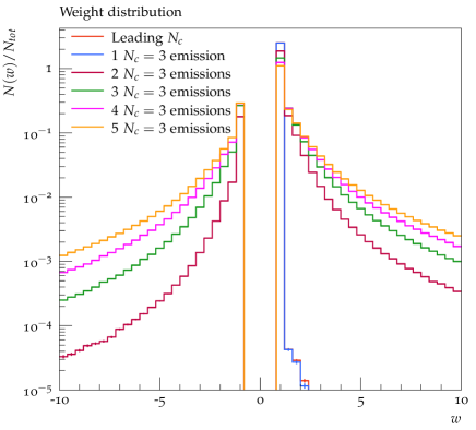
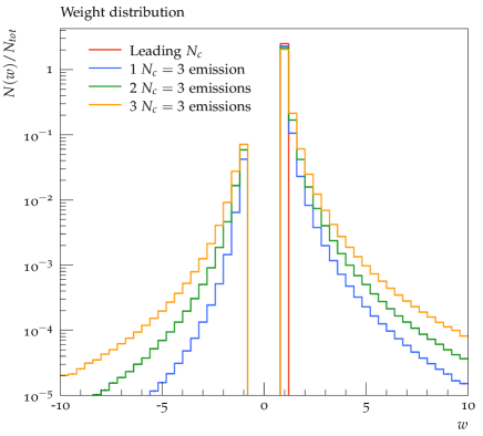
Figure 1: Weight distribution for $e^{+}e^{-}$ (left) and $pp$ collisions (right) depending on the number of $N_{c}=3$ emissions allowed. All generated events are used in these plots, i.e., no further analysis cut is applied.

In figure 1 we show the weight distribution for up to five/three subleading $N_{c}$ emissions at LEP/LHC respectively corresponding to up to six/seven $q\overline{q}$-pairs plus gluons in the color bases. We note that although the weight distributions get broader with the number of emissions, it stays sufficiently narrow to ensure convergence for the considered number of subleading emissions. The number of colored partons, which we can practically include, is therefore limited by the evaluation of scalar products in color space, as described in section 4. (We will find, however, that we are able to keep sufficiently many full color emissions for standard hard observables to converge.)

Somewhat against intuition, we see a broader weight distribution for LEP events than for LHC events, despite the fact that we tend to have more colored partons at the LHC. This can be attributed to the fact that the corrections often tend to be negative at LEP (starting from $e^{+}e^{-}\rightarrow q\overline{q}$), due to the negative contribution from coherent emission from the $q\overline{q}$-pair. In line with this, we also note that if we separately study $qq\rightarrow qq$, $qg\rightarrow qg$ and $gg\rightarrow gg$, we find the largest weight variations for $qq\rightarrow qq$, another case where we can expect large negative corrections from $q\overline{q}$-pairs.

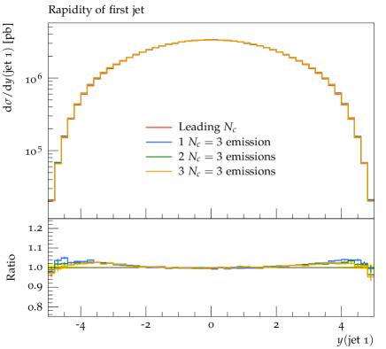
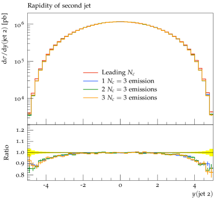
Figure 2: Rapidity distribution of the first and second jet as zero, one, two and three $N_{c}=3$ emissions are kept.

We next turn to the convergence of standard observables with respect to the number of subleading $N_{c}$ corrected emissions. As an example, we consider the rapidities of the hardest LHC jets in figure 2. As can be seen, the curves converge as more subleading emissions are added, and in this respect we see the same pattern for all standard hard LHC observables; they all converge when up to three subleading emissions are added, i.e., starting with a $2\rightarrow 2$ topology and adding three subleading emissions (followed by leading $N_{c}$ showering) gives results very similar to adding just two subleading $N_{c}$ emissions (followed by leading $N_{c}$ showering). LEP observables show a similar convergence pattern. Only when explicitly considering very many jets, does the convergence fail. This strongly suggests that for standard hard observables, subleading $N_{c}$ corrections can be well approximated by color correcting the first few emissions.

The convergence can also be underpinned by studying the evolution scale at which the $N_{c}=3$ parton shower terminates, and further evolution only is given by the leading $N_{c}$ shower. This is investigated in figure 3 where the transverse momentum, as measured in the frame of the emitting dipole, is shown in orange for the last full color corrected emission, i.e., while keeping up to three subleading emissions at the LHC and up to five subleading emissions at LEP. For comparison we also show the distribution of the first emission not to be corrected.

We find that the typical scale of the last color corrected emission is about 1 GeV at LEP and about 5-10 GeV at LHC, using a 50 GeV cut. Increasing the cut to 1 TeV gives a much harder last subleading $N_{c}$ corrected emission, as expected.

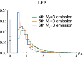
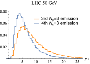
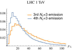
Figure 3: Transverse momentum distribution in the dipole frame of the last $N_{c}=3$ emission (orange) and the first non-corrected emission (blue). For LEP the second-to-last $N_{c}=3$ emission is also shown (green). For LHC we use a 50 GeV (middle) and a 1 TeV (right) cut on the hardest parton. The shower cut-off at LEP is 0.45 GeV, and events which reach this scale are shown in the 0-bin above.

The convergence of observables is also in line with results from a very recent paper on subleading $N_{c}$ corrections at LEP Isaacson:2018zdi , where the authors claim to observe good convergence while keeping subleading corrections down to a variable cut-off at around 3 GeV.

In Isaacson:2018zdi a Monte Carlo sampling over color is advocated, and the point is made that this avoids the factorial scaling in color space. In view of figure 3, we note, however, that we can go further down in $p_{\perp}$ despite keeping the full color structure. In fact, even if we limit ourselves to four subleading $N_{c}$ emissions, for which the time penalty due to color structure treatment is negligible, we also go well below 3 GeV. Therefore, in the case of hard observables at LEP, color structure sampling seems to be of no benefit for the convergence of observables.

We have also performed a number of standard shower variation checks, including shower scale variation and infrared cutoff variation. While varying the shower scale, we find effects very similar to the leading $N_{c}$ case. Increasing the infrared cutoff from 1 to 2 GeV likewise results in differences well comparable to the leading $N_{c}$ shower, and so does adding multiple interactions.

Finally, we have checked what happens if the shower is turned off completely after one to three subleading emissions. Here, we find large differences for the LHC, even if we keep up to three subleading $N_{c}$ corrected emissions. We therefore conclude that it is essential to keep showering beyond three color corrected emissions, but it is — for standard hard QCD observables, or likely any observable which is mostly sensitive to the hardest jets — not important to keep color correcting the subsequent, softer and softer, emissions. For observables depending on soft physics, the situation may be different, as indicated below.

7.2 LEP — final state radiation

7.2.1 Parton level analyses

We first recapitulate the exercise from Platzer:2012np and run an $e^{+}e^{-}$ simulation at $\sqrt{s}=91.2$ GeV, without hadronization, but this time including subsequent leading $N_{c}$ showering beyond the (up to) five subleading $N_{c}$ emissions, as well as $g\rightarrow q\overline{q}$ splittings. Again we find that the corrections to most LEP observables are small. As examples of observables which show some effect, we show the fraction of events containing $n$ jets with $E>5$ GeV, the thrust distribution, and the aplanarity in figure 4, in all cases showing corrections below 10%.

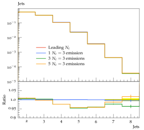
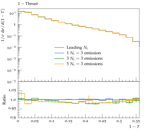
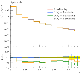
Figure 4: Parton level plots for fraction of LEP-events containing $n$ jets with $E>5$ GeV (left), thrust (middle) and aplanarity (right), the jets have been clustered with the anti-$k_{\perp}$-type generalized $e^{+}e^{-}$ clustering algorithm with $R=0.7$. For hadronized events the effect on thrust vanishes, whereas the effects on number of jets and aplanarity are somewhat reduced. Note that the case of one full $N_{c}$ emission should agree with the leading $N_{c}$ shower, as is seen.

On the other hand, effects can be significant in tailored situations. For example, considering the average transverse momentum with respect to a thrust axis defined by the three hardest partons, we find corrections above 10%. We caution, however, that without modification this is not an observable.

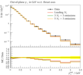
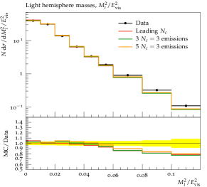
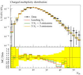
Figure 5: Out-of-plane $p_{\perp}$ w.r.t. the thrust and thrust major axes (left), light hemisphere mass (middle) and fraction of events containing $N_{\mathrm{ch}}$ charged particles, using to data and Rivet analyses from Abreu:1996na ; Barate:1996fi .

7.2.2 Hadron level

We have studied hadronized LEP events for a large class of observables from Abreu:1996na ; Barate:1996fi . For planarity, sphericity, oblateness, and in- and out-of-plane $p_{\perp}$ w.r.t. sphericity axis, we find small differences of a few percent or less, whereas C-parameter shows some effects of 5-10% in the low C-parameter region. As examples, in figure 5, we show the total out-of-plane $p_{\perp}$ (w.r.t. the plane defined by the thrust and thrust major axes) and the light hemisphere mass in comparison to data from Abreu:1996na .

In general the deviation of simulated results compared to data from Abreu:1996na ; Barate:1996fi ; Heister:2003aj is clearly dominated by other factors, and the overall description of data does not change visibly. Turning, on the other hand, to observables sensitive to soft physics, we find larger differences. As an example we show the charged multiplicity distribution in figure 5 (right), compared to data from Barate:1996fi , but we likewise see large effects for Durham jet resolution variables in the soft region, on the color singlet cluster masses for the Herwig hadronization model Bahr:2008pv and on individual hadron multiplicities.

While it is tempting to interpret the charged particle multiplicity plot in figure 5, as improved data description, we remark that the hadronization model in use, is the standard Herwig cluster hadronization model Bahr:2008pv , with a leading $N_{c}$ color flow, as described in section 3. We therefore caution that the differences should only be seen as an indication of effects on soft physics, from the altered particle kinematics entering the hadronization. While this can be interpreted as a need to retune the full color parton shower, retuning shower parameters is beyond the scope of the present paper.

7.3 LHC — coherent initial and final state radiation

7.3.1 Parton level analyses

We now turn to the LHC and start with reconsidering figure 2. Considering the leading two jets, with our standard $p_{\perp}>50$ GeV analysis cut, we see that they tend to have slightly different rapidity distributions, with the second jet being more central. For most other standard observables we find small differences, of a few percent or less. Nevertheless it is illustrative to separately consider scattering involving different partons. Doing so we find that for $qq\rightarrow qq$ and $gg\rightarrow gg$, the subleading $N_{c}$ corrections are small for all studied observables, whereas for $qg\rightarrow qg$, they can be more sizable. In figure 6 we therefore revisit the rapidity distributions of the two leading jets, and find corrections going in opposite directions for the two jets. Since $qg$-induced scattering contributes with a large fraction of the cross section for the applied cuts, and since LHC data contains $qg\rightarrow qg$ and $gq\rightarrow gq$ (along with all other processes), it can be concluded that significant cancellation of subleading $N_{c}$ corrections is present at LHC.

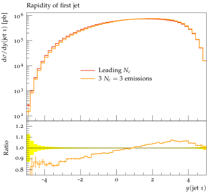
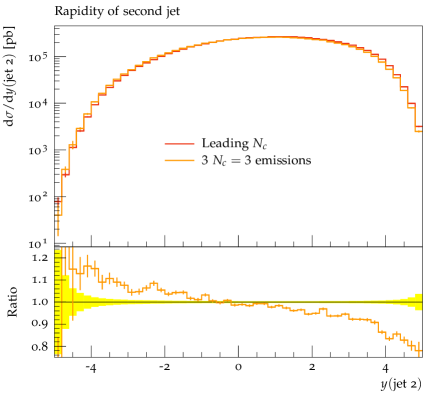
Figure 6: Rapidity distribution of the hardest and second hardest jet while considering only $qg\rightarrow qg$ scattering.

Using the cuts of radek.simon ,

$$400\text{ GeV} <M_{12}<600\text{ GeV}\ ,$$

$$3.8 <|y_{1}+y_{2}|<5.2\ ,$$ (22)

$$1.5 <|y_{2}-y_{1}|<3.5\ ,$$

where $y_{1}$ and $y_{2}$ are the rapidities of the hardest and second hardest jet and $M_{12}$ is the invariant mass of the two hardest jets, events dominated by the hard process $qg\rightarrow{}qg$ can be statistically enhanced. These cuts select events with one of the two hardest jets being forward (in either direction) and one central. With these cuts we find differences of $5-10\%$ for the rapidity distributions of the hardest three jets, as illustrated in figure 7 for the hardest jet. From figure 7, we see that in the $N_{c}=3$ shower, the hardest jet tends to be central less often as compared to the leading $N_{c}$ shower. The rapidity distribution of the second hardest jet shows that it is forward less often. There are also $5-10\%$ differences in $\Delta\phi_{ij}=\phi_{i}-\phi_{j}$, $\Delta\eta_{ij}=\eta_{i}-\eta_{j}$ and $\Delta{}R_{ij}=\sqrt{\Delta\phi_{ij}^{2}+\Delta\eta_{ij}^{2}}$, for $i=1,2\ ,j=3$. As an example $\Delta{}\phi_{13}$ is also shown in figure 7. In general, with these cuts subleading $N_{c}$ effects show sizable corrections for many standard QCD observables.

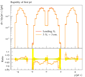
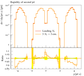
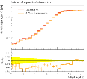
Figure 7: Rapidity distribution of the hardest jet (left), second hardest jet (middle) and separation in $\phi$ of the hardest and third hardest jets (right). Our standard analysis cut of $p_{\perp}>50$ GeV is used.

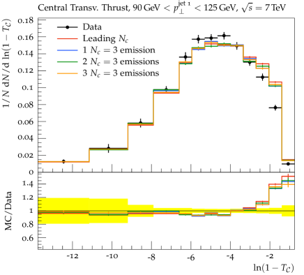
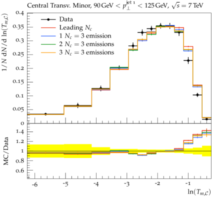
Figure 8: Distribution of $\log_{e}(1-T_{C})$ (left) and $T_{m,c}$ (right) for $\sqrt{s}=7$GeV. Data and Rivet analysis are taken from Khachatryan:2011dx .

7.3.2 Hadron level analyses

We now turn our attention to hadronized events and to comparisons with LHC data. We have compared the subleading $N_{c}$ corrected parton shower to experimental data for a wide range of QCD observables, using data from Khachatryan:2011dx ; Aad:2012meb ; ATLAS:2012al ; Aad:2013fba ; Chatrchyan:2013fha ; Aad:2014pua ; Aad:2016ria . First, in figure 8, we consider the event shape central transverse thrust, defined as Banfi:2010xy

$$T_{C}=\mbox{max}_{\hat{n}_{T}}\frac{\sum_{i}|\overline{p}_{\perp,i}\cdot\hat{n}_{T}|}{\sum_{i}p_{\perp,i}}\,,$$ (23)

where $p_{\perp,i}$ is the transverse momentum of the central jet $i$, having pseudorapidity $\eta<1.3$, and $\hat{n}_{T}$ is the direction perpendicular to the beam axis, which maximizes the sum. We also consider central thrust minor, defined again in terms of central jets with $\eta<1.3$,

$$T_{m,C}=\frac{\sum_{i}|\overline{p}_{\perp,i}\times\hat{n}_{T}|}{\sum_{i}p_{\perp,i}}\,,$$ (24)

and compare to data from Khachatryan:2011dx . As can be seen we find relatively small corrections, at the 5% level or below.

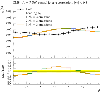
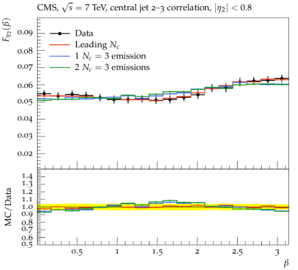
Figure 9: The angle $\beta$, defined as in eq. (25) using (left) an underlying $2\rightarrow 2$ hard process and (right) an underlying $2\rightarrow 3$ hard process. Data and Rivet analysis are taken from Chatrchyan:2013fha .

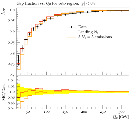
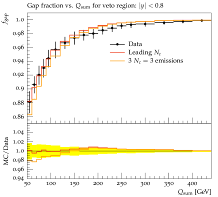
Figure 10: Fraction of events having no additional jet with $p_{\perp}$ above $Q_{0}$ within a rapidity interval $|y|<0.8$ (left) and fraction of events where the scalar sum of transverse momenta within $|y|<0.8$ does not exceed $Q_{\mathrm{sum}}$ (right) for $t\overline{t}$ events at $\sqrt{s}=7$ TeV. Data and Rivet analysis are taken from ATLAS:2012al .

A comparison to the jet shapes and jet masses for high $p_{\perp}$ jets, from Aad:2012meb , shows yet smaller subleading $N_{c}$ corrections, typically below a few percent.

We have also compared data to the so-called color coherence effects from Chatrchyan:2013fha . In figure 9 we show the distribution of the $\beta$-angle, defined in terms of the pseudorapidities $\eta_{2}$ and $\eta_{3}$ and the azimuthal angles $\phi_{2}$ and $\phi_{3}$, as

$$\tan{\beta}=\frac{|\phi_{3}-\phi_{2}|}{\mbox{sign}(\eta_{2})(\eta_{3}-\eta_{2})}\,.$$ (25)

Experimental data is first compared to shower predictions using a $2\rightarrow 2$ hard matrix element, and then using a $2\rightarrow 3$. We clearly see that the use of a $2\rightarrow 3$ hard matrix element significantly improves the description of data, whereas adding subleading $N_{c}$ showering to the $2\rightarrow 2$ process changes the distribution compared to the leading $N_{c}$ shower very marginally. This casts doubt upon the description of this observable as probing color coherence, and rather illustrates its dependence on the hard matrix element (or alternatively on other details of the shower algorithm).

We have also investigated the effects from subleading color contributions on top-pair production, and compared to data from ATLAS:2012al ; Aad:2013fba . Here we find that the jet shapes from Aad:2013fba are essentially unaltered, whereas the measurement of the additional jet activity in $t\overline{t}$ events ATLAS:2012al show intriguing effects, displayed in figure 10. In particular we note that the data description improves in the region of a modest ratio between $Q_{0}/Q_{\mathrm{sum}}$ and the hard scale. For gap observables, like in figure 10, with a large scale hierarchy, we remark that we can expect effects from resummation of virtual gluons, which we do not include in this paper. These subleading $N_{c}$ corrections may be sizable Forshaw:2007vb ; Cox:2010ug ; DuranDelgado:2011tp ; Martinez:2018ffw .

As a clean test of initial state radiation, we have also compared the $N_{c}=3$ shower to event shapes in leptonic $Z$ decay events, Aad:2016ria . Here, as expected, having fewer colored particles in the hard process, we find very small corrections, at the percent level or below.

8 Conclusion and outlook

In this paper we have investigated the effect of keeping the full color structure in parton shower emissions in realistic simulations of LHC and LEP events. This is pursued within the dipole shower of the Herwig 7.1 framework Bellm:2017bvx as color matrix element corrections.

The $N_{c}=3$ color shower corrects the first few (five for LEP and three for LHC) emissions using the full $N_{c}=3$ emission pattern. All hard observables we have studied, with the exception of observables explicitly considering very many jets, have converged with respect to keeping additional subleading $N_{c}$ color corrected emissions. The convergence can also be underpinned by noting that the last emission to be corrected, corresponds to a low evolution scale, in comparison to the studied observables, see figure 3. In particular for LEP, we typically go down to evolution scales around one GeV.

Our results show that, for most QCD variables at the LHC, the subleading $N_{c}$ effects are, similarly to at LEP, of the order of a few percent. At the LHC we can, however, see larger effects, $10-20\%$, for the tails of the rapidity distribution of the second hardest jet, figure 2, as well as for more tailored situations, c.f. figure 7.

In a gedanken experiment, where quarks and gluons are collided, larger differences can be found, indicating that cancellation of subleading $N_{c}$ effects are present at the LHC. To capture this situation, we consider LHC events while requiring that of the two most energetic jets, one is central and one is forward. In this case we find differences of $5-10\%$ also for standard QCD observables. These differences are not only in the tails of the distributions, but over the whole range of several observables.

Turning to soft observables the situation is different. In many cases, including jet resolution variables at low scales, charged particle multiplicities (figure 5), individual hadron multiplicities and the number of very soft jets at LEP, we find large effects, of several 10%. While we cannot expect to make accurate predictions for any of these cases, due to sensitivity to hadronization, multiple interaction and resummation effects, it should be stressed that subleading $N_{c}$ effects can be expected to play an important role for the final state of the shower, entering the hadronization. An immediate extension of this work is therefore retuning of the $N_{c}=3$ shower. Indeed, an improved description to (most) observables cannot be expected until retuning is performed.

Another natural next step is to include virtual corrections. Virtual gluon exchanges would allow rearrangement of the color structure without emission. This would be expected to have an effect on gap fraction observables, such as in figure 10, and we therefore caution that our conclusions regarding the magnitude of the subleading $N_{c}$ corrections may not be applicable in these cases.

More precisely, virtual gluon exchanges should be the mechanism underlying (perturbative) color reconnection effects. In the longer perspective, it would be desirable to update the standard hadronization model to encompass a subleading $N_{c}$ shower.

For these reasons, we like to stress that this work should be considered as the start of subleading $N_{c}$ corrections at the LHC, not the end. Indeed much work remains to be done.

Note added

While this work has been finalized, a similar approach has been reported in Isaacson:2018zdi . In Isaacson:2018zdi color matrix element corrections, as well as the weighted Sudakov algorithm for final state evolution is used, but a sampling of color structure is advocated.

Appendix A Choices for the modified veto algorithm

This appendix contains the details for the choice of acceptance probability and overestimate kernel for the modified weighted Sudakov veto algorithm. The arguments of the splitting kernels, $p_{\perp}^{2},z,p_{\tilde{ij}}$ and $p_{\tilde{k}}$, have been suppressed for clarity in the following equations.

We use the modified version of the weighted sudakov veto algorithm from Bellm:2016voq , as described in section 5. The splitting kernel we aim at generating, ${\cal P}_{ij,k}$, is given in eq. (17). Defining ${\cal P}_{ij,k}^{N_{c}\rightarrow\infty}$ to be the leading color limit of ${\cal P}_{ij,k}$, assuming $\tilde{ij}$ and $\tilde{k}$ are color connected (cf. eq. (8)), and letting ${\cal R}_{ij,k}^{N_{c}\rightarrow\infty}$ be the standard overestimate used in Herwig, as obtained from the ExSample Platzer:2011dr adapted grid proposal, we can write

$${\cal P}_{ij,k}=\text{sign}(\omega_{\tilde{ij}\,\tilde{k}}^{n})|\omega_{\tilde{ij}\,\tilde{k}}^{n}|(1+\delta_{\tilde{ij}}){\cal P}_{ij,k}^{N_{c}\rightarrow\infty}\ .$$ (26)

Our choice for the overestimate kernel is ${\cal R}_{ij,k}=|\omega_{\tilde{ij}\,\tilde{k}}^{n}|(1+\delta_{\tilde{ij}}){\cal R}_{ij,k}^{N_{c}\rightarrow\infty}$ and our choice for the acceptance probability is

$$\epsilon=\frac{|{\cal P}_{ij,k}|}{{\cal R}_{ij,k}}=\frac{{\cal P}_{ij,k}^{N_{c}\rightarrow\infty}}{{\cal R}_{ij,k}^{N_{c}\rightarrow\infty}}\ ,$$ (27)

i.e. we use the same acceptance probability as for the leading $N_{c}$ shower (if $\tilde{ij}$, $\tilde{k}$ were color connected). The acceptance weight is then

$$\text{sign}(\omega_{\tilde{ij}\,\tilde{k}}^{n})\,=\left\{\begin{matrix}1&\text{ for $\omega_{\tilde{ij}\,\tilde{k}}^{n}>0$}\\ -1&\text{ for $\omega_{\tilde{ij}\,\tilde{k}}^{n}<0$}\\ \end{matrix}\right.\ ,$$ (28)

and the veto weight is

$$\frac{{\cal R}_{ij,k}^{N_{c}\rightarrow\infty}-\text{sign}(\omega_{\tilde{ij}\,\tilde{k}}^{n}){\cal P}_{ij,k}^{N_{c}\rightarrow\infty}}{{\cal R}_{ij,k}^{N_{c}\rightarrow\infty}-{\cal P}_{ij,k}^{N_{c}\rightarrow\infty}}=\left\{\begin{matrix}1&\text{ for $\omega_{\tilde{ij}\,\tilde{k}}^{n}>0$}\\ \frac{{\cal R}_{ij,k}^{N_{c}\rightarrow\infty}+{\cal P}_{ij,k}^{N_{c}\rightarrow\infty}}{{\cal R}_{ij,k}^{N_{c}\rightarrow\infty}-{\cal P}_{ij,k}^{N_{c}\rightarrow\infty}}&\text{ for $\omega_{\tilde{ij}\,\tilde{k}}^{n}<0$}\\ \end{matrix}\right.\ .$$ (29)

From eq. (28) and eq. (29) we see that trial emissions corresponding to positive $\omega_{\tilde{ij}\,\tilde{k}}^{n}$ never change the event weight.

References

- (1) T. Sjöstrand, S. Mrenna and P. Skands, A Brief Introduction to PYTHIA 8.1, Comput. Phys. Commun. 178 (2008) 852 [0710.3820].
- (2) M. Bahr et al., Herwig++ Physics and Manual, Eur. Phys. J. C58 (2008) 639 [0803.0883].
- (3) J. Bellm et al., Herwig 7.0/Herwig++ 3.0 release note, Eur. Phys. J. C76 (2016) 196 [1512.01178].
- (4) T. Gleisberg et al., SHERPA 1.alpha, a proof-of-concept version, JHEP 02 (2004) 056 [hep-ph/0311263].
- (5) S. Plätzer and M. Sjodahl, The Sudakov Veto Algorithm Reloaded, Eur. Phys. J. Plus 127 (2012) 26 [1108.6180].
- (6) S. Plätzer, ExSample: A Library for Sampling Sudakov-Type Distributions, Eur. Phys. J. C72 (2012) 1929 [1108.6182].
- (7) S. Plätzer and S. Gieseke, Dipole Showers and Automated NLO Matching in Herwig++, 1109.6256.
- (8) S. Plätzer, Controlling inclusive cross sections in parton shower + matrix element merging, JHEP 08 (2013) 114 [1211.5467].
- (9) J. Bellm, S. Gieseke and S. Plätzer, Merging NLO Multi-jet Calculations with Improved Unitarization, 1705.06700.
- (10) M. Dasgupta, F. A. Dreyer, K. Hamilton, P. F. Monni and G. P. Salam, Logarithmic accuracy of parton showers: a fixed-order study, 1805.09327.
- (11) L. Lönnblad, Correcting the colour-dipole cascade model with fixed order matrix elements, JHEP 05 (2002) 046 [hep-ph/0112284].
- (12) F. Krauss, Matrix elements and parton showers in hadronic interactions, JHEP 08 (2002) 015 [hep-ph/0205283].
- (13) S. Hoeche, F. Krauss, N. Lavesson, L. Lonnblad, M. Mangano et al., Matching parton showers and matrix elements, hep-ph/0602031.
- (14) N. Lavesson and L. Lönnblad, Merging parton showers and matrix elements – back to basics, JHEP 04 (2008) 085 [0712.2966].
- (15) S. Hoeche, F. Krauss, S. Schumann and F. Siegert, QCD matrix elements and truncated showers, JHEP 05 (2009) 053 [0903.1219].
- (16) K. Hamilton, P. Richardson and J. Tully, A modified CKKW matrix element merging approach to angular-ordered parton showers, 0905.3072.
- (17) M. Dobbs, Phase space veto method for next-to-leading order event generators in hadronic collisions, Phys. Rev. D65 (2002) 094011 [hep-ph/0111234].
- (18) S. Frixione and B. R. Webber, Matching NLO QCD computations and parton shower simulations, JHEP 06 (2002) 029 [hep-ph/0204244].
- (19) P. Nason, A new method for combining NLO QCD with shower Monte Carlo algorithms, JHEP 11 (2004) 040 [hep-ph/0409146].
- (20) Z. Nagy and D. E. Soper, Matching parton showers to NLO computations, JHEP 10 (2005) 024 [hep-ph/0503053].
- (21) S. Frixione, F. Stoeckli, P. Torrielli and B. R. Webber, NLO QCD corrections in Herwig++ with MC@NLO, JHEP 1101 (2011) 053 [1010.0568].
- (22) S. Plätzer and M. Sjodahl, Subleading improved parton showers, JHEP 1207 (2012) 042 [1201.0260].
- (23) Z. Nagy and D. E. Soper, Parton shower evolution with subleading color, JHEP 06 (2012) 044 [1202.4496].
- (24) Z. Nagy and D. E. Soper, Effects of subleading color in a parton shower, JHEP 07 (2015) 119 [1501.00778].
- (25) S. Plätzer, Summing Large- Towers in Colour Flow Evolution, Eur. Phys. J. C74 (2014) 2907 [1312.2448].
- (26) R. Á. Martínez, M. De Angelis, J. R. Forshaw, S. Plätzer and M. H. Seymour, Soft gluon evolution and non-global logarithms, 1802.08531.
- (27) J. Bellm et al., Herwig 7.1 Release Note, 1705.06919.
- (28) S. Plätzer and S. Gieseke, Coherent Parton Showers with Local Recoils, JHEP 01 (2011) 024 [0909.5593].
- (29) S. Catani and M. Seymour, The Dipole formalism for the calculation of QCD jet cross-sections at next-to-leading order, Phys.Lett. B378 (1996) 287 [hep-ph/9602277].
- (30) S. Catani and M.H. Seymour, A general algorithm for calculating jet cross sections in NLO QCD, Nucl. Phys. B485 (1997) 291 [hep-ph/9605323].
- (31) K. Cormier, S. Plätzer, C. Reuschle, P. Richardson and S. Webster , in preparation.
- (32) S. Catani, S. Dittmaier, M. H. Seymour and Z. Trocsanyi, The Dipole formalism for next-to-leading order QCD calculations with massive partons, Nucl. Phys. B627 (2002) 189 [hep-ph/0201036].
- (33) G. Gustafson and U. Pettersson, Dipole Formulation of QCD Cascades, Nucl. Phys. B306 (1988) 746.
- (34) J. Bellm, Colour Rearrangement for Dipole Showers, Eur. Phys. J. C78 (2018) 601 [1801.06113].
- (35) T. Sjöstrand, A Model for Initial State Parton Showers, Phys. Lett. 157B (1985) 321.
- (36) J. E. Paton and H.-M. Chan, Generalized Veneziano model with isospin, Nucl. Phys. B 10 (1969) 516.
- (37) F. A. Berends and W. Giele, The Six Gluon Process as an Example of Weyl-Van Der Waerden Spinor Calculus, Nucl. Phys. B294 (1987) 700.
- (38) M. L. Mangano, S. J. Parke and Z. Xu, Duality and multi-gluon scattering, Nucl. Phys. B 298 (1988) 653.
- (39) M. L. Mangano, The color structure of gluon emission, Nucl. Phys. B 309 (1988) 461.
- (40) D. A. Kosower, Color Factorization for Fermionic Amplitudes, Nucl. Phys. B315 (1989) 391.
- (41) Z. Nagy and D. E. Soper, Parton showers with quantum interference, JHEP 09 (2007) 114 [0706.0017].
- (42) M. Sjodahl, Color structure for soft gluon resummation – a general recipe, JHEP 0909 (2009) 087 [0906.1121].
- (43) J. Alwall, M. Herquet, F. Maltoni, O. Mattelaer and T. Stelzer, MadGraph 5 : Going Beyond, JHEP 1106 (2011) 128 [1106.0522].
- (44) M. Sjodahl, ColorFull – a C++ library for calculations in SU(Nc) color space, Eur. Phys. J. C75 (2015) 236 [1412.3967].
- (45) A. Kyrieleis and M. H. Seymour, The colour evolution of the process , JHEP 01 (2006) 085 [hep-ph/0510089].
- (46) Y. L. Dokshitzer and G. Marchesini, Soft gluons at large angles in hadron collisions, JHEP 01 (2006) 007 [hep-ph/0509078].
- (47) M. Sjodahl, Color evolution of 2 3 processes, JHEP 12 (2008) 083 [0807.0555].
- (48) M. Beneke, P. Falgari and C. Schwinn, Soft radiation in heavy-particle pair production: All-order colour structure and two-loop anomalous dimension, Nucl. Phys. B 828 (2010) 69 [0907.1443].
- (49) S. Keppeler and M. Sjodahl, Orthogonal multiplet bases in SU(Nc) color space, JHEP 09 (2012) 124 [1207.0609].
- (50) Y.-J. Du, M. Sjodahl and J. Thorén, Recursion in multiplet bases for tree-level MHV gluon amplitudes, JHEP 05 (2015) 119 [1503.00530].
- (51) M. Sjodahl and J. Thorén, Decomposing color structure into multiplet bases, JHEP 09 (2015) 055 [1507.03814].
- (52) G. ’t Hooft, A PLANAR DIAGRAM THEORY FOR STRONG INTERACTIONS, Nucl. Phys. B72 (1974) 461.
- (53) A. Kanaki and C. G. Papadopoulos, HELAC-PHEGAS: Automatic computation of helicity amplitudes and cross-sections, hep-ph/0012004.
- (54) F. Maltoni, K. Paul, T. Stelzer and S. Willenbrock, Color flow decomposition of QCD amplitudes, Phys. Rev. D 67 (2003) 014026 [hep-ph/0209271].
- (55) J. Bellm, S. Plätzer, P. Richardson, A. Siódmok and S. Webster, Reweighting Parton Showers, Phys. Rev. D94 (2016) 034028 [1605.08256].
- (56) M. Cacciari, G. P. Salam and G. Soyez, The Anti-k(t) jet clustering algorithm, JHEP 04 (2008) 063 [0802.1189].
- (57) A. Buckley, J. Butterworth, L. Lonnblad, D. Grellscheid, H. Hoeth, J. Monk et al., Rivet user manual, Comput. Phys. Commun. 184 (2013) 2803 [1003.0694].
- (58) J. Isaacson and S. Prestel, On stochastically sampling color configurations, 1806.10102.
- (59) DELPHI collaboration, P. Abreu et al., Tuning and test of fragmentation models based on identified particles and precision event shape data, Z. Phys. C73 (1996) 11.
- (60) ALEPH collaboration, R. Barate et al., Studies of quantum chromodynamics with the ALEPH detector, Phys. Rept. 294 (1998) 1.
- (61) ALEPH collaboration, A. Heister et al., Studies of QCD at e+ e- centre-of-mass energies between 91-GeV and 209-GeV, Eur. Phys. J. C35 (2004) 457.
- (62) S. Gieseke, S. Plätzer and R. Podskubka in preparation.
- (63) CMS collaboration, V. Khachatryan et al., First Measurement of Hadronic Event Shapes in Collisions at TeV, Phys. Lett. B699 (2011) 48 [1102.0068].
- (64) ATLAS collaboration, G. Aad et al., ATLAS Measurements of the Properties of Jets for Boosted Particle Searches, Phys. Rev. D86 (2012) 072006 [1206.5369].
- (65) ATLAS collaboration, G. Aad et al., Measurement of production with a veto on additional central jet activity in pp collisions at sqrt(s) = 7 TeV using the ATLAS detector, Eur. Phys. J. C72 (2012) 2043 [1203.5015].
- (66) ATLAS collaboration, G. Aad et al., Measurement of jet shapes in top-quark pair events at = 7 TeV using the ATLAS detector, Eur. Phys. J. C73 (2013) 2676 [1307.5749].
- (67) CMS collaboration, S. Chatrchyan et al., Probing color coherence effects in pp collisions at , Eur. Phys. J. C74 (2014) 2901 [1311.5815].
- (68) ATLAS collaboration, G. Aad et al., Measurements of jet vetoes and azimuthal decorrelations in dijet events produced in collisions at using the ATLAS detector, Eur. Phys. J. C74 (2014) 3117 [1407.5756].
- (69) ATLAS collaboration, G. Aad et al., Measurement of event-shape observables in events in collisions at 7 TeV with the ATLAS detector at the LHC, Eur. Phys. J. C76 (2016) 375 [1602.08980].
- (70) A. Banfi, G. P. Salam and G. Zanderighi, Phenomenology of event shapes at hadron colliders, JHEP 06 (2010) 038 [1001.4082].
- (71) J. R. Forshaw and M. Sjodahl, Soft gluons in Higgs plus two jet production, JHEP 09 (2007) 119 [0705.1504].
- (72) B. E. Cox, J. R. Forshaw and A. D. Pilkington, Extracting Higgs boson couplings using a jet veto, Phys. Lett. B696 (2011) 87 [1006.0986].
- (73) R. M. Duran Delgado, J. R. Forshaw, S. Marzani and M. H. Seymour, The dijet cross section with a jet veto, JHEP 08 (2011) 157 [1107.2084].