The Fermi bubbles from stochastic acceleration of electrons in a Galactic outflow

The discovery of the Fermi bubbles—a huge bilobular structure seen in GeV gamma-rays above and below the Galactic center—implies the presence of a large reservoir of high energy particles at $\sim 10\,\text{kpc}$ from the disk. The absence of evidence for a strong shock coinciding with the edge of the bubbles, and constraints from multi-wavelength observations point towards stochastic acceleration by turbulence as a likely mechanism of acceleration. We have investigated the time-dependent acceleration of electrons in a large-scale outflow from the Galactic centre. For the first time, we present a detailed numerical solution of the particle kinetic equation that includes the acceleration, transport and relevant energy loss processes. We also take into account the addition of shock acceleration of electrons at the bubble’s blast wave. Fitting to the observed spectrum and surface brightness distribution of the bubbles allows determining the transport coefficients, thereby shedding light on the origin of the Fermi bubbles.

1 Introduction

The detection of the Fermi bubbles–a huge bi-lobular structure seen in GeV gamma-rays–is certainly one of the great discoveries made with the Fermi-LAT instrument. Due to their position on the sky (see below), they are likely emanating from the Galactic centre and the most speculated about sources are the supermassive black hole at the Galactic centre and star formation/star burst in the Galactic centre region. These processes shape Galactic structure on the largest scales and as such the Fermi bubbles allow us to study Galactic feedback in our own backyard. Furthermore, given their prominence in gamma-rays, they are an important arena for studies of sources of diffuse GeV emissions, like searches for signals from self-annihilation or decay of dark matter. Finally, the production of the gamma-rays and the acceleration of the underlying particles are of astrophysical interest in itself.

1.1 Observational properties

Originally the Fermi bubbles were observed in a search (Dobler et al. 2010) for the gamma-ray counterpart of a microwave excess seen from the inner Galaxy (Finkbeiner 2004; Dobler & Finkbeiner 2008; Ade et al. 2013). A more detailed analysis (Su et al. 2010) unveiled some surprising properties that were later largely confirmed by Ackermann et al. (2014). In the following we summarise the most important observational properties of the Fermi bubbles in gamma-rays.

Geometry:

The Fermi bubbles are approximately centered at zero Galactic longitude, symmetric about the Galactic plane, $50^{\circ}$ wide in longitude with each bubble extending up to $50^{\circ}$ in latitude, see, e.g. Fig. 22 of Ackermann et al. (2014). On these scales, they constitute the first evidence for an outflow from the Milky Way. (On smaller scales, there had previously been evidence in X-rays in an X-shaped feature around the Galactic centre.) The bubbles’ symmetry about the Galactic plane and their being centred around zero longitude imply an origin at Galactic centre (distance $d_{GC}\simeq 8.5\,\text{kpc}$). A wind with a constant speed of $1000\,\text{km}\,\text{s}^{-1}$ would need about $9.9\,\text{Myr}$ to expand into a bubble of size $\sim d_{GC}\tan 50^{\circ}\simeq 10.1\,\text{kpc}$, modulus projection effects: At a latitude of $50^{\circ}$, we might be seeing the limb-brightened edge of a bubble of radius $d_{GC}\sin 50^{\circ}\simeq 6.5\,\text{kpc}$, thus reducing the time-scale to $6.4\,\text{Myr}$. Note that because the eastern edge of the northern bubble is very close to the position of the North-polar spur, which is part of the the radio Loop I. Initially, this led to claims of the bubbles being associated with the Loop I structure (Casandjian & Grenier 2009).

Spectrum:

The gamma-ray flux shows a hard spectrum, mostly $\propto E^{-2}$ and extending from a few hundred MeV up to a few hundred GeV, see, e.g. Fig. 18 of Ackermann et al. (2014). At lower energies, the spectrum is significantly harder, and at high energies there is evidence for a spectral softening or an exponential cut-off. This spectral shape immediately invites speculation about its physical origin, i.e. whether the gamma-rays are of leptonic (from inverse-Compton scattering) or hadronic ($\pi^{0}$ decay) origin. (Given the estimates of the physical conditions, inside the bubbles, see below, bremsstrahlung is most likely negligible.)

While the spectral shoulder around a few hundred MeV determined in the earlier analysis (Su et al. 2010) seemed to be well fit by the kinematic feature from $\pi^{0}$ decay, the new best-fit spectrum appears to be extending to lower energies. Likely, a hadronic model needs to have a spectral break (a steeper spectrum of the underlying protons) at lower energies. This is in addition to the required spectral break or cut-off at high energies. The physical origin of these breaks is a priori unclear.

In leptonic models these breaks are easily explained. The inverse-Compton spectrum is naturally rather hard: In the Thomson regime, a gamma-ray spectrum $\propto\epsilon^{-s}$ with ($s\sim 2)$ with a cutoff at $\epsilon_{\rm cut}$ of a few hundred GeV can be produced by an electron spectrum $\propto E^{-\Gamma}\mathrm{e}^{-E/E_{\mathrm{cut}}}$ with $\Gamma=2s-1\sim 3$ and $E_{\mathrm{cut}}=/m_{\mathrm{e}}c^{2}\sqrt{\epsilon/\epsilon_{\rm soft}}\sim 1,500$ GeV for soft photon energies of $\epsilon\sim 1$ eV. Note that these estimates are strictly only valid in the Thomson regime. In the numerical computations, however, we have used the full Klein-Nishina cross-section and taken into account the relativistic corrections.

Surface brightness.

The surface brightness shows little variation over the bubbles, but has sharp edges as can already be seen in the residual map, cf. e.g. Fig. 29 of Ackermann et al. (2014). More quantitatively, this is evidenced by profiles of the gamma-ray flux across the bubble edge, shown e.g. in Fig. 22 of Ackermann et al. (2014). There is clearly a jump in intensity from a value close to zero (after template subtraction) outside to a relatively constant value inside the bubbles. In fact, the only substructure seen is a rather large enhancement of emissivity in the east of the southern bubble, called the “cocoon”, the origin of which is of yet unknown. There have also been claims of evidence for a narrow and extendend, jet-like feature (Su & Finkbeiner 2012), however, the analysis by the Fermi collaboration (Ackermann et al. 2014) has found this feature not to be significant.

The flat surface brightness and sharp edges are one of the most puzzling features of the bubbles. The sharp edges require an efficient confinement of the gamma-ray producing particles and the flat surface brightness requires a peculiar distribution of volume emissivity. Idealising each bubble as a spherically symmetric volume with outer radius $R$, only an emissivity that varies with radius $r$ as $1/\sqrt{1-(r/R)^{2}}$ will give a flat surface brightness and sharp edges.

Spectral uniformity.

The bubbles show similar morphologies in different energy bins ranging from $1$ to $500\,\text{GeV}$ (see e.g. Fig. 22 of Ackermann et al. (2014)) or equivalently the spectrum is uniform in different parts of the bubbles. Specifically, the gamma-ray spectrum has been analyzed in different latitude bands and the spectrum in the bubble edge region and the interior have been compared: For the latitude bands, no variation has been found above and below $\pm 10^{\circ}$. Between $-10^{\circ}$ and $+10^{\circ}$ there is an excess at the Galactic Centre (Hooper & Slatyer 2013), likely with a spherical symmetry, and its connection to the Fermi bubbles is unclear at this point (Ackermann et al. 2017). Furthermore, no variation between the edge region and the interior was found (Su et al. 2010) (but see also Keshet & Gurwich (2017)).

The spectral uniformity is also very surprising for such an extended structure. Leptonic models in particular would be expected to lead to some variation, depending on the region of energizing of the high-energy electrons. This is due to cooling losses by synchrotron radiation and inverse-Compton emission. A conservative estimate of the cooling time is $\tau_{\text{cool}}=6.74\times 10^{8}\text{yr}\,(E/\text{GeV})^{-1}((u_{B}+u_{\text{CMB}})/(0.486\,\text{eV}\text{cm}^{-3}))^{-1}$, for magnetic fields and radiation fields of energy densities $u_{B}=0.224\,\text{eV}\,\text{cm}^{-3}(B/3\mu\text{G})^{2}$ and $u_{\text{CMB}}=0.262\,\text{eV}\,\text{cm}^{-3}$, respectively, i.e. of the same order as the bubble age for $100\,\text{GeV}$ electrons. Therefore, electrons energised in the Galactic plane will be subject to considerable cooling while travelling out into the bubble volume. This results in softer spectra at larger distances from the Galactic centre and thus a softer gamma-ray spectrum at higher latitudes. In addition, the energy densities in the radiation backgrounds that the electron inverse-Compton scatter on should be varying with distance from the disk: While the CMB is of course spatially uniform, the energy densities in both the optical/UV and the infrared backgrounds should become smaller further away from the disk. The fact that this is not observed imply that the variation in the radiation backgrounds must be counter-balanced by a variation in the electron spectrum to some degree.

1.2 Hints

While the discovery of the Fermi bubbles was certainly a surprise, it was not the first hint at the presence of Galaxy-scale outflows. Kiloparsec-scale outflows have been observed for starburst galaxies, e.g. in ionised gas. Even in our own Milky Way, there had been hints at the presence of a Galaxy-scale outflow, possibly connected with high-energy cosmic rays: Observations in soft X-rays, most notably from ROSAT, showed signs of an x-shaped feature, interpreted as evidence of a biconical outflow in analogy with structures seen in other galaxies.

The presence of a population of high-energy cosmic ray electrons was already hinted at by the microwave haze, an excess of microwaves from the Galactic centre, pointing at a similarly hard electron spectrum (Finkbeiner 2004; Dobler & Finkbeiner 2008; Ade et al. 2013). (Note, however, the possible influence of systematic effects due to template subtraction (Mertsch & Sarkar 2010).) The search for a counterpart of the microwave haze in gamma-rays was in fact what motivated the first study that lead to the discovery of the Fermi bubbles (Dobler et al. 2010).

1.3 Other constraints

X-rays.

A number of studies have investigated the properties of the thermal gas in the Fermi bubbles and in the Galactic halo from X-ray observations. The parameters can be either inferred from the thermal, soft X-ray spectrum (Kataoka et al. 2013, 2015) or from individual Oxygen lines (Miller & Bregman 2016). The gas densities inferred are of the order $n_{\text{gas}}\sim 10^{-3}\,\text{cm}^{-3}$ and the temperatures of the gas just outside the bubbles vary between $kT\simeq 0.3\,\text{keV}$ and $0.5\,\text{keV}$. This is higher than the canonical temperature of the Galactic halo of $kT\simeq 0.2\,\text{keV}$ and requires a heating agent, perhaps a weak shock with a low Mach number; $\mathcal{M}\simeq 1.5\mathellipsis 2.3$. Finally, with the typical sound speed in the Galactic halo of $c_{s}\simeq 200\,\text{km}\,\text{s}^{-1}$, one infers shock speeds of $v_{\rm sh}\simeq 300\mathellipsis 500\,\text{km}\,\text{s}^{-1}$.

The absence of evidence for a strong shock coinciding with the bubble edge implies that diffusive shock acceleration at the bubble edge cannot be the primary mechanism of acceleration. If electrons get accelerated in the Galactic plane or even in a hypothetical large-scale jet along the Galactic minor axis, they need to travel over distances of several kpc without much energy loss to fill the bubble volume. As a result they will suffer severe cooling losses and a gradual softening of their spectrum, or even quench the electron density completely. Note further that the low shock speeds found by the X-ray modeling lead to even larger dynamical times than with the $1000\,\text{km}\,\text{s}^{-1}$ assumed above, making the energy losses even more important.

Quasar absorption.

The observation of absorption by the gas associated with the bubbles from a background quasar can also be used to set bounds on the outflow speed. In the UV absorption lines from PDS 456 two (asymmetric) components with velocities of $v\simeq-235$ and $+250\,\text{km}\,\text{s}^{-1}$ with respect to the local standard of rest could be identified (Miller & Bregman 2016). For the conical outflow assumed in that study, this implies an upper limit on the outflow speed of $\gtrsim 900\,\text{km}\,\text{s}^{-1}$. This seems to be in conflict with the shock speed inferred from the X-ray modelling described above. Note, however, that the outflow speed inferred from the absorption lines of one quasar is very dependent on the assumed geometry of the flow. Future observations of additional sight lines towards other quasars can help mapping out the flow structure, thus possibly also constraining it geometry, and might bring the results into agreement with the values inferred from X-rays.

1.4 Models

The Fermi bubbles have also generated a great deal of interest on the modelling side (Crocker & Aharonian 2011; Cheng et al. 2011, 2012; Zubovas et al. 2011; Mertsch & Sarkar 2011; Zubovas & Nayakshin 2012; Guo & Mathews 2012; Yang et al. 2012; Lacki 2014; Crocker et al. 2014; Fujita et al. 2013; Thoudam 2013; Yang et al. 2013; Crocker et al. 2014; Fujita et al. 2014; Cheng et al. 2014, 2015a; Mou et al. 2014; Crocker et al. 2015; Cheng et al. 2015b; Mou et al. 2015; Sarkar et al. 2015; Sasaki et al. 2015; Yang & Ruszkowski 2017). The variety of models is most conveniently classified by:

• the source of energy: super massive black hole or stellar winds/supernovae;

• the acceleration region: jet or sources in the disk or in situ (by shocks or turbulence);

• the nature of the high-energy particles: hadrons or leptons.

Of course, the individual options are not mutually exclusive. For instance, in hadronic models, the bulk of the high-energy gamma-rays comes from decay of neutral pions. Charged pions, however, get produced at similar rates and can, given the radiation fields, their $e\pm$ byproducts can inverse-Compton scatter soft photons into low energy gamma-rays. However, in this particular scenario the synchrotron spectrum would be too soft (Ackermann et al. 2014)

As a full discussion of all proposed models is beyond the scope of this highlight presentation, only two particular classes of models will be presented, and a few concrete examples will be shown.

Jet models.

Astrophysical jets are thought to be powered by accretion onto a spinning, compact object, like neutron stars or black holes. Given the position and symmetry of the Fermi bubbles, the supermassive black hole at the Galactic centre is a prime candidate. Although conspicuously quiet (its X-ray luminosity is currently more than 11 orders below the Eddington luminosity), there is indirect evidence for earlier epochs of active accretion, e.g. from X-ray reflections.

Jets are usually associated with high speeds $\gtrsim 1000\,\text{km}\,\text{s}^{-1}$. This allows for the electrons to be less impacted by energy losses than in starburst/star formation models and therefore the source of energisation of the high-energy electrons can be in the Galactic disk or inside the jet. (Note, however, that the jet speed is not necessarily directly implying the dynamical age as the bubbles can be formed by a fountain-like back flow due to the termination of the jet by the ram pressure of gas in the Galactic halo.)

One of the earliest studies of a leptonic jet model employing a hydrodynamical simulation (Guo & Mathews 2012) found that the lateral extent of the Fermi bubbles could be explained if the jet was underdense but slightly overpressured. If active at $10\,\%$ of the Eddington luminosity for $1-2\,\text{Myr}$ until about a Myr ago, the morphology would match the observations. A subsequent MHD simulation of the Fermi bubbles blown up by a jet (Yang et al. 2012) showed further that the shock compression at the bubble edges would compress the magnetic field such that it gets aligned with the bubble edge. We will return to this point in Sec. 2.3.

Star formation/star burst models.

The Galactic winds that get collectively powered by an ensemble of stellar winds or supernova activity, are usually operating at smaller speeds, $\lesssim 500\,\text{km}\,\text{s}^{-1}$. This implies a larger dynamic time-scales than for the jet model, leading to a preference in the literature for hadronic models, as leptons would cool too fast. In hadronic models, on the other hand, cosmic rays need to be accumulated over much longer time scales, given the low gas densities of the order of $10^{-3}\,\text{cm}^{-3}$ (see Sec. 1.3), to produce the observed gamma-ray fluxes. In turn, this and the observed hard $E^{-2}$ spectrum require an effective confinement of the high-energy cosmic rays to the bubbles and a suppression of (energy-dependent) escape. (See, however, Keshet & Gurwich (2017).) The sources of high energy particles are nevertheless oftentimes assumed to be in the Galactic disk.

The most detailed numerical star formation/star burst model for the Fermi bubbles as of yet (Sarkar et al. 2015) employs a hydrodynamical code to investigate the interaction of a Galactic wind with the circumgalactic medium. It is found that a luminosity of $5\times 10^{40}\,\text{erg}\,\text{s}^{-1}$ and a density in the halo of $10^{-3}\,\text{cm}^{-3}$ can reproduce the morphology observed in gamma-rays and is also in agreement with X-ray observations. Interestingly, this luminosity is close to the one inferred from the current star formation rate, $\text{SFR}\simeq 0.007\mathellipsis 0.1M_{\odot}\,\text{yr}^{-1}$, when assuming an efficiency of $30\,\%$ for conversion into mechanical power, $\mathcal{L}\simeq 10^{40}\text{erg}\,\text{s}^{-1}\varepsilon_{0.3}(\text{SFR}/(0.1M_{\odot}\,\text{yr}^{-1}))$.

The outflow from the inner Galaxy leads to a shock structure known from the heliosphere or supernova remnants, with a radial forward shock at $\sim 11\,\text{kpc}$, a more tangled contact discontinuity extending to $\sim 8\,\text{kpc}$ above the Galactic centre and a very much tangled reverse shock a few kiloparsecs inside of the contact discontinuity. Thus, in this model, the edge of the gamma-ray bubble does not coincide with the projection of the forward shock, but rather the contact discontinuity. Whether this is due to the diffusion prescription of Sarkar et al. (2015) changing across the contact discontinuity would need to be explored further.

1.5 Motivation

The observation of $\gamma$-rays from the bubbles implies a huge reservoir of high-energy particles in the Galactic halo, but the source and the mechanism of acceleration of these particles has not been established thus far. Other sources of non-thermal particles, like supernova remnants, pulsar wind nebulae, jets in active galaxies or winds in starburst galaxies, show evidence of shocks through X-rays or ionization lines. The Fermi bubbles, however, show no such evidence of a (strong) shock, raising the question of the possible mechanism of acceleration. Acceleration by plasma turbulence (or “stochastic acceleration”, SA), however, can fill the bubbles with high-energy electrons. (See, Petrosian (2012) for a recent review of SA.

A first SA model for the Fermi bubbles (Mertsch & Sarkar 2011) was presented quickly after their discovery. This model was employing the solution of a simplified version of the transport equation. Specifically, diffusion was ignored as a spatial transport process and advection was the only transport process. In this framework, cosmic ray electrons are just passively advected with the downstream flow while being stochastically accelerated. The time scale hierarchy $t_{\text{dyn}}\gg t_{\text{cool}}\gg t_{\text{acc}}$ of dynamical, cooling and acceleration times, allows a steady-state solution of the variation of electron spectrum with radius for a given spatial variations of theses and and the escape time, $t_{\text{esc}}$. While successful in explaining the overall spectrum of the bubbles as well as the sharp edges, the lack of diffusive transport was an important shortcoming. In addition, the interstellar radiation fields on which the cosmic ray electrons scatter was assumed homogeneous which must be an oversimplification. What is needed is a detailed numerical model, taking into account all the spatial transport processes (diffusion, advection), energy losses (ionisation, bremsstrahlung, synchrotron, inverse Compton scattering) and energy gains (shock and SA).

In the remainder of this paper, we will present our computation of the SA of high-energy electrons in the Fermi bubbles. Sec. 2 introduces our method for solving the transport equation on a grid that is suited for the geometry of the bubbles. We will define three setups and specify the parameter values considered. We will show our result for those three setups in Sec. 3 and comment on compatibility with observational data. In Sec. 4 we summarise and conclude.

2 Method

2.1 Transport equation

We start by considering the following transport equation for the (isotropic) phase space density $f(\@vec{r},p,t)$, e.g. (Blandford & Eichler 1987),

$$\frac{\partial f}{\partial t}=\nabla\cdot\left(K\cdot\nabla f-\@vec{V}f\right)+\frac{1}{p^{2}}\dfrac{\partial}{\partial p}\left(p^{2}D_{pp}\dfrac{\partial f}{\partial p}\right)$$

$$+\frac{1}{p^{2}}\dfrac{\partial}{\partial p}p^{2}\left(\frac{p}{3}\left(\nabla\cdot\@vec{V}\right)f\right)\,.$$ (1)

Here, spatial transport is governed by the diffusion tensor $K$ and the advection velocity $\@vec{V}$, the latter also leading to adiabatic gains/losses through the divergence term. Momentum space diffusion depends on the diffusion coefficient $D_{pp}$.

For numerical convenience, we reformulate eq. 1 in terms of $\psi=4\pi p^{2}\times f$, the differential (in momentum) particle density which is related to the total particle density $n=\int\mathrm{d}p\,\psi$. We also add momentum and catastrophic losses $-\partial(\dot{p}\psi)/\partial p$ and $-\psi/\tau$ and a source term $S$,

$$\frac{\partial\psi}{\partial t}=\nabla\cdot\left(K\cdot\nabla\psi-\@vec{V}\psi\right)+\dfrac{\partial}{\partial p}\left(p^{2}D_{pp}\dfrac{\partial}{\partial p}\frac{\psi}{p^{2}}\right)$$

$$+\dfrac{\partial}{\partial p}\left(-\dot{p}\psi+\frac{p}{3}\left(\nabla\cdot\@vec{V}\right)\psi\right)-\frac{\psi}{\tau}+S\,.$$ (2)

2.2 Shock equation

At the shock, we need to carefully evaluate the transport eq. 2 because of the discontinuity in $\@vec{V}$ (and in other transport parameters). We denote quantities upstream (downstream) of the shock by a minus (plus) sign. We demand $\psi$ to be continuous across the shock,

$$\psi^{-}=\psi^{+}\,,$$

and allow for the presence of sources at the shock, $S^{*}\delta(\@vec{r}-\@vec{r}_{\text{sh}})$, so that by continuity

$$\nabla\cdot\@vec{J}=S^{*}\delta(\@vec{r}-\@vec{r}_{\text{sh}})\,.$$

With Gauss’ theorem, we can write this as

$$\int_{V}\mathrm{d}V\,(\nabla\cdot\@vec{J})=\int_{A}\mathrm{d}\@vec{A}\cdot\@vec{J}=\int_{V}\mathrm{d}V\,S^{*}\delta(\@vec{r}-\@vec{r}_{\text{sh}})\,.$$ (3)

The particle density flux $\@vec{J}$ is here

$$\@vec{J} =-\hat{n}K_{\parallel}(\hat{n}\cdot\nabla)\psi+\frac{1}{3}\left(2-\frac{\partial\ln\psi}{\partial\ln p}\right)\@vec{V}\psi\,.$$ (4)

For numerical solution of the transport and shock equations, we need to specify a coordinate system.

2.3 Coordinates

A convenient choice of coordinates should help simplify the computation, e.g. in that it eases or altogether eliminates the transformation from the simulation coordinates to the frame in which the diffusion tensor is diagonal. The method for treating the discontinuity of the shock requires that the shock normal to be aligned with one coordinate direction.

Given the bi–lobular shape of the bubbles as observed in gamma–rays (Su et al. 2010; Ackermann et al. 2014) and used in the (M)HD simulations (Guo & Mathews 2012; Yang et al. 2012), leads us to employ toroidal coordinates ($u,v,\phi$) which map to cartesian coordinates ($x,y,z$) through

$$x =\frac{a\sinh{v}\cos{\phi}}{\cosh{v}-\cos{u}}\,,$$ (5)

$$y =\frac{a\sinh{v}\sin{\phi}}{\cosh{v}-\cos{u}}\,,$$ (6)

$$z =\frac{a\sin{u}}{\cosh{v}-\cos{u}}\,.$$ (7)

In Fig. 1, we show a plot of surfaces of constant $u$ and $v$. Surfaces of constant $u$ are spheres of varying radii that all intersect a foci ring of radius $a$. Surfaces of constant $v$ are tori of varying radii surrounding the foci ring. We set $a=1\,\text{kpc}$ throughout unless otherwise noted.

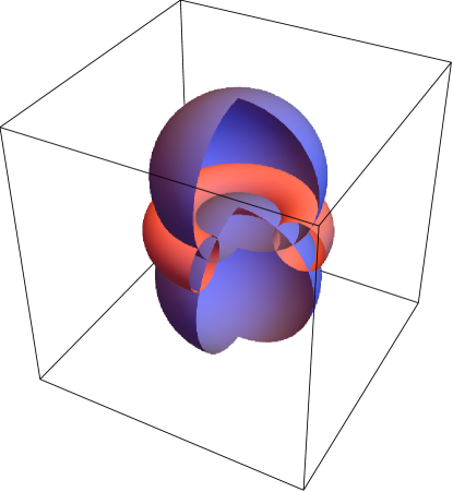
Figure 1: Toroidal coordinates. Surfaces of constant $v$ are tori of varying radii surrounding the foci ring of radius $a$ and are shown in red. Surfaces of constant $u$ are spheres of varying radii that all intersect the foci ring and are shown in blue.

From the transformation between cartesian and toroidal coordinates, eqs. 5 - 7, we can compute the scale factors

$$h_{u} =h_{v}=\frac{a}{\cosh v-\cos u}\,\quad\text{and}\quad h_{\phi} =\frac{a\sinh v}{\cosh v-\cos u}\,.$$ (8)

Here and in the following, we assume azimuthal ($\phi$) symmetry and also define the cylindrical radial coordinate $\rho=\sqrt{x^{2}+y^{2}}$.

2.3.1 Transport equation in toroidal coordinates

We can write the transport equation 2 in toroidal coordinates,

$$\frac{\partial\psi}{\partial t} =\left[\frac{(\cosh v-\cos u)^{2}}{a^{2}}K_{uu}\right]\frac{\partial^{2}\psi}{\partial u^{2}}$$

$$+\left[-\frac{(\cosh v-\cos u)\sin u}{a^{2}}K_{uu}+\frac{(\cosh v-\cos u)^{2}}{a^{2}}\dfrac{\partial K_{uu}}{\partial u}\right]\frac{\partial\psi}{\partial u}$$

$$+\left[-\frac{\cosh v-\cos u}{a}V_{u}\right]\frac{\partial\psi}{\partial u}$$

$$+\left[\frac{(\cosh v-\cos u)^{2}}{a^{2}}K_{vv}\right]\frac{\partial^{2}\psi}{\partial v^{2}}$$

$$+\left[\frac{(\cosh v-\cos u)(1-\cosh v\cos u)}{a^{2}\sinh v}K_{vv}\right.$$

$$\quad\quad\left.+\frac{(\cosh v-\cos u)^{2}}{a^{2}}\dfrac{\partial K_{vv}}{\partial v}\right]\frac{\partial\psi}{\partial v}$$

$$+D_{pp}\dfrac{\partial^{2}\psi}{\partial p^{2}}+\left[\dfrac{\partial D_{pp}}{\partial p}-\frac{2}{p}D_{pp}\right]\dfrac{\partial\psi}{\partial p}$$

$$+\left[-\dot{p}+\frac{p}{3}(\nabla\cdot\@vec{V})\right]\dfrac{\partial\psi}{\partial p}$$

$$+\left[\frac{2}{p^{2}}D_{pp}-\frac{2}{p}\dfrac{\partial D_{pp}}{\partial p}-\dfrac{\partial\dot{p}}{\partial p}-\frac{2}{3}(\nabla\cdot\@vec{V})-\frac{1}{\tau}\right]\psi+S\,.$$ (9)

A comment about the velocity divergence,

$$\nabla\cdot\@vec{V}=\frac{(\cosh v-\cos u)^{3}}{a^{3}\sinh v}\dfrac{\partial}{\partial u}\left(\frac{a^{2}\sinh v}{(\cosh v-\cos u)^{2}}V_{u}\right)\,,$$

is in order. For an incompressible flow, $0\equiv\nabla\cdot\@vec{V}$, but if we want fronts to follow lines of constant $u$, then we require the $v$–dependence (see, discussion in Sec. 2.6.1 below)

$$V_{u}\propto h_{u}=\frac{a}{\cosh v-\cos u}\,.$$

Note that in eq. 9

$$\frac{(\cosh v-\cos u)(1-\cosh v\cos u)}{a^{2}\sinh v}\frac{\partial\psi}{\partial v}$$ (10)

is indeterminate for $v\to 0$ as $\sinh v\to 0$ and $\partial\psi/\partial v\to 0$ (due to symmetry). Employing the L’Hopital’s rule, we can replace this by

$$\frac{(\cosh v-\cos u)(1-\cosh v\cos u)}{a^{2}\cosh v}\frac{\partial^{2}\psi}{\partial v^{2}}$$ (11)

2.3.2 Shock equation in toroidal coordinates

If the shock is in the $u$–plane and the flux is perpendicular to the shock, $\@vec{J}=J_{u}\hat{u}$, eq. 3 reads

$$\quad J_{u}^{+}-J_{u}^{-}=\lim_{\epsilon\to 0}\int_{u_{\text{sh}}-\epsilon}^{u_{\text{sh}}+\epsilon}\mathrm{d}u\,h_{u}S^{*}\delta(u-u_{\text{sh}})=h_{u}S^{*}\,,$$ (12)

where (cf. eq. 4)

$$J_{u}=-K_{uu}\frac{1}{h_{u}}\dfrac{\partial\psi}{\partial u}+\frac{1}{3}\left(2-\frac{\partial\ln\psi}{\partial\ln p}\right)V_{u}\psi\,.$$ (13)

We thus find,

$$-\left(\frac{1}{h_{u}}V_{u}^{-}-\frac{1}{h_{u}}V_{u}^{+}\right)\frac{1}{3}\left(2\psi-p\dfrac{\partial\psi}{\partial p}\right)$$

$$+\left(\frac{K_{uu}^{-}}{h_{u}^{2}}\left(\dfrac{\partial\psi}{\partial u}\right)^{-}-\frac{K_{uu}^{+}}{h_{u}^{2}}\left(\dfrac{\partial\psi}{\partial u}\right)^{+}\right) =S^{*}(p)\,,$$ (14)

2.4 Finite–difference method

Parabolic partial differential equations like the transport equation 2 are oftentimes solved numerically by finite difference methods. Here, we numerically solve the transport equation in toroidal coordinates (cf. eq. 9) in the widely used Crank–Nicolson scheme (Crank et al. 1947). This is a semi–implicit method which results in a tridiagonal system that can be efficiently solved by the Thomas algorithm. The difficulty in the case at hand is the presence of the shock which breaks the tridiagonality of the involved matrix. In particular at the shock position, we solve the shock equation 14 instead of the transport equation 9. Here we follow a method outlined by Langner (2004) which treats transport in the heliosphere in the presence of the helioshperic termination shock.

2.5 Computational grid

The computational grid is three–dimensional: two spatial, toroidal coordinates ($u$ and $v$) and one momentum coordinate ($p$). Choosing the spatial grids to be linear renders the coefficients for the finite difference scheme particularly simple and offers the added advantage of fine resolution close the Galactic centre and at the bases of the bubbles. For the momentum grid we chose logarithmic spacing in order to evenly sample the spectra which will be close to power law:

$$u_{i} =u_{\mathrm{min}}+i\Delta r=u_{\mathrm{min}}+\frac{i}{n}(u_{\mathrm{max}}-u_{\mathrm{min}})\,,\quad i=0,\mathellipsis n,$$ (15)

$$v_{j} =v_{\mathrm{min}}+j\Delta\theta=v_{\mathrm{min}}+\frac{j}{m}(v_{\mathrm{max}}-v_{\mathrm{min}})\,,\quad j=0,\mathellipsis m,$$ (16)

$$p_{k} =p_{\mathrm{min}}\mathrm{e}^{k\Delta\ln p}=p_{\mathrm{min}}\mathrm{e}^{k\left[\ln\left(p_{\mathrm{max}}/p_{\mathrm{min}}\right)\right]/q}\,,\quad k=0,\mathellipsis q.$$ (17)

For the minimum and maximum coordinate values and number of grid points, we need to balance accuracy and computational speed under the constraint of suppressing numerical artefacts, e.g. oscillations. Here, we have chosen the following grid parameters:

$$\begin{array}[]{rlrlrl}u_{\text{min}}&=0\,,&u_{\text{max}}&=\pi\,,&n&=800\,,\\ v_{\text{min}}&=0\,,&v_{\text{max}}&=2\,,&m&=40\,,\\ cp_{\text{min}}&=10^{-3}\,\text{GeV}\,,&cp_{\text{max}}&=10^{4}\,\text{GeV}\,,&q&=140\,.\\ \end{array}$$ (18)

For $u_{\text{max}}=\pi$ and $v_{\text{max}}\to\infty$, the computational domain is covering the whole $\rho$–$z$ plane. To limit the size of the grid while assuming linear spacing, we limit $v_{\text{max}}$ to finite values. This will affect the transport and acceleration of particles close to $\rho=1\,\text{kpc}$; however, due to the presence of strong diffuse, conventional emission, the Galactic disk is usually excluded from diffuse studies, cf., e.g., (Su et al. 2010; Ackermann et al. 2014).

The spatial part of the computational grid is shown in Fig. 2.

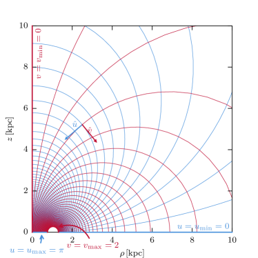
Figure 2: The spatial part of the computational grid. Note that for clarity, we only show $n=100$ spacings in the $u$–direction here, whereas in the numerical simulations, we have chosen $n=800$ throughout. Note also that the use of $v_{\rm max}=2$ instead of $\infty$ ignores a small region of space.

2.6 Parameters

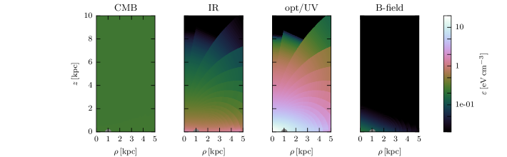
Figure 3: Energy densities $\varepsilon$ of the CMB, IR and optical/UV parts of the ISRF as well as the energy density of the $B$–field in the $\rho$–$z$–plane. We define the energy ranges as $4.3\times 10^{-5}$ to $1.4\times 10^{-2}\,\text{eV}$ for the CMB, $1.4\times 10^{-2}$ to $0.22\,\text{eV}$ for the IR and $0.22$ to $14\,\text{eV}$ for the optical/UV.

Diffusion is only really isotropic in the limit of a small regular magnetic field $B_{0}$, i.e. when the fractional turbulence level $\eta=\delta B^{2}/(B_{0}^{2}+\delta B^{2})\to 1$. In the general case, the symmetric part of the diffusion tensor $K$ can be written as $K=\text{diag}(K_{\perp},K_{\perp},K_{\parallel})$ in cartesian coordinates where without loss of generality we have assumed that $\@vec{B}_{0}\parallel\hat{z}$. In quasi–linear theory, $K_{\parallel}$ and $K_{\perp}$ scale differently with the turbulence level $\eta)$; $K_{\parallel}\propto\eta^{-1}$ while $K_{\perp}\propto\eta$. In our case, we assume $\@vec{B}_{0}\parallel\hat{v}$ and so $K_{\perp}=K_{uu}\propto\eta$ and $K_{\parallel}=K_{vv}\propto\eta^{-1}$, and adopt a momentum dependence consistent with resonant interactions with Kolmogorov turbulence,

$$K=\left(\begin{array}[]{cc}K_{uu}&0\\ 0&K_{vv}\end{array}\right)\quad\text{with}\quad K_{uu} =\beta K_{uu,0}\left(\frac{pc}{1\,\text{GeV}}\right)^{\delta}$$ (21)

$$\text{and}\quad K_{vv} =\beta K_{vv,0}\left(\frac{pc}{1\,\text{GeV}}\right)^{\delta}\,.$$ (22)

For the momentum diffusion coefficient, we are employing a relation from quasi–linear theory,

$$K_{\parallel}D_{pp}\approx p^{2}V_{A}^{2}\,,$$ (23)

where $V_{A}$ is the Alfvén speed. This fixes the momentum dependence of $D_{pp}$,

$$D_{pp}=\beta^{-1}D_{pp,0}\left(\frac{pc}{1\,\text{GeV}}\right)^{2-\delta}\,,$$ (24)

and parametrises its normalisation relative to $K_{\parallel}$ through the Alfvén speed $V_{A}\simeq B_{0}/\sqrt{4\pi m_{p}n_{\text{gas}}}$,

$$D_{pp,0}= \frac{V_{A}^{2}}{K_{\parallel}}\left(\frac{\text{GeV}}{c}\right)^{2}$$ (25)

$$\simeq \left(\frac{V_{A}}{300\,\text{km}\,\text{s}^{-1}}\right)^{2}\left(\frac{K_{\parallel}}{3\times 10^{28}\,\text{cm}^{2}\,\text{s}^{-1}}\right)^{-1}$$ (26)

$$\quad\times\left(\frac{\text{GeV}}{c}\right)^{2}\text{Myr}^{-1}\,.$$ (27)

We assume the shock to follow an isocontour in $u$ and in order for advection fronts to follow lines of constant $u$, we choose the advection velocity $\@vec{V}=V_{u}\hat{u}$ and its absolute value proportional to the scale factor $h_{u}=a/(\cosh v-\cos u)$. We introduce an additional $u$–dependence, $(1-\cos u)$, and define the compression ratio $r$ of the shock, that is the ratio of upstream to downstream speed in the shock frame, such that

$$V_{u}=-\left(1-\frac{1}{r}\right)V_{\text{sh}}\frac{a(1-\cos u)}{\cosh v-\cos u}\,,$$ (28)

This results in the shock travelling with constant speed $V_{\text{sh}}$ along the $z$–axis:

$$\frac{\mathrm{d}u}{\mathrm{d}t}=\frac{\cosh v-\cos u}{a}V_{u} =-V_{\text{sh}}(1-\cos u)\,,$$

$$\Leftrightarrow-\cot(u/2)+\cot(u_{0}/2) =-V_{\text{sh}}(t-t_{0})\,.$$

With $t_{0}=0$ and $u_{0}=u(t_{0})=\pi$,

$$u_{\text{sh}}(t)=2\,\mathrm{arccot}(V_{\text{sh}}t)\,,$$

and one finds

$$z(u_{\text{sh}}(t),0)=\frac{a\sin u_{\text{sh}}(t)}{1-\cos u_{\text{sh}}(t)}=\frac{a\sin(2\,\mathrm{arccot}V_{\text{sh}}t)}{1-\cos(2\,\mathrm{arccot}V_{\text{sh}}t)}=V_{\text{sh}}t\,.$$

With the $V_{\text{sh}}=3\times 10^{-7}\,\text{kpc}\,\text{yr}\simeq 300\,\text{km}\,\text{s}^{-1}$ that we adopt, the shock reaches a height of $z=6\,\text{kpc}$ in $t=20\,\text{Myr}$. And with the $u$–dependence in eq. ( 28) we get

$$\nabla\cdot\@vec{V}=\left(1-\frac{1}{r}\right)V_{\text{sh}}\sin u\left(1-3\frac{(1-\cos u)}{\cosh v-\cos u}\right)\,.$$

Here, we set the compression ratio to $4$, but it is strictly only so along the $z$–axis.

One can estimate the timescales for shock acceleration and stochastic acceleration as $\tau_{\rm sh}\sim K_{uu}/V_{\text{sh}}^{2}$ and $\tau_{\rm SA}\sim p^{2}/D_{pp}\sim K_{vv}/V_{A}^{2}$ with the ratio is $(\tau_{\rm sh}/\tau_{\rm SA})\sim(K_{uu}/K_{vv})V_{A}^{2}/V_{\text{sh}}^{2}=(\eta/{\cal M}_{A})^{2}$, where ${\cal M}_{A}$ is the Alfv́en Mach number. (see, Petrosian 2012). In the following, we adopt $V_{A}=300\,\text{km}\text{s}^{-1}$ everywhere. The shock velocity, however, is not constant along the shock as the bubble expands more slowly laterally than vertically. At the top, $v_{\text{sh}}=300\,\text{km}\text{s}^{-1}$ which coincides with the Alfvén speed and thus the rates for shock acceleration and stochastic acceleration will be equal for isotropic diffusion ($K_{uu}=K_{vv}$). For anisotropic diffusion ($K_{uu}<K_{vv}$), shock acceleration even operates faster than stochastic acceleration. In contrast, at the foot of the bubble, the shock velocity is much lower than the Alfvén speed, rendering shock acceleration inefficient. Note that in either case, the effective volume where shock acceleration operates is rather small because of the small diffusion length $K_{uu}/V_{u}$.

We idealise the shock as a surface of constant pseudo–radius $u$. Furthermore, we assume that the (large–scale) $B$–field (which defines the coordinate system in which the diffusion tensor is diagonal) is aligned with these surface of constant $u$, that is $\@vec{B}\parallel\hat{v}$ where $\hat{v}$ is the unit vector of the pseudo–polar coordinate, $v$.

The interstellar radiation fields (ISRFs) affect both the momentum losses of the electrons and the generation of gamma–rays through inverse–Compton scattering (Blumenthal & Gould 1970). Here we adopt a model (Porter & Strong 2005) from version 50 of the GALPROP code (Moskalenko & Strong 1998; Orlando & Strong 2013). This contains the energy density of the ISRF on a grid in cylindrical coordinates. We bilinearly interpolate from the cylindrical grid to our toroidal grid. As the cylindrical grid only extends to $z=\pm 5\,\text{kpc}$, we linearly extrapolate for $|z|>5\,\text{kpc}$, but set the ISRF to zero if it were otherwise negative. The left three panels of Fig. 3 show the energy densities in the CMB, IR and UV/optical ranges as a function of $\rho$ and $z$.

The coherent magnetic field is assumed to follow lines of constant $u$ (see above), that is $\@vec{B}\parallel\hat{v}$, but we only use this to define the coordinates in which the diffusion tensor is diagonal. For synchrotron losses and the computation of radio/microwave fluxes we ignore the regular field for the time being. Instead, we only consider a turbulent component with rms value

$$B_{\text{rms}}(\rho,z)=B_{0}\exp\left[-\frac{\rho}{\rho_{0}}-\frac{z}{z_{0}}\right]\,.$$ (29)

Here and in the following, we choose the set of parameters $B_{0}=3\,\mu\text{G}$, $\rho_{0}=5\,\text{kpc}$ and $z_{0}=1\,\text{kpc}$ as a fiducial model. The energy density of this turbulent magnetic field is shown in the rightmost panel of Fig. 3.

For the source term $Q$, we simply adopt a Dirac delta function, both in position and in momentum,

$$Q(\rho,z,p)\propto\delta(\@vec{r})\delta(p)\,.$$ (30)

The normalisation is determined by fitting to the gamma–ray data from Fermi–LAT (Ackermann et al. 2014). Specifically, we require the maximum gamma-ray flux in our map at $10\,\text{GeV}$ to be $E^{2}J=8\times 10^{-7}\mathrm{GeV}\,\mathrm{cm}^{-2}\,\mathrm{s}^{-1}\,\mathrm{sr}^{-1}$.

In principle we would have liked to also investigate the possibility of accelerating electrons from the thermal background. However, for an ambient temperature $T$ this would have required extending the momentum grid down to thermal momenta of the order $pc\simeq k_{B}T\simeq 8.6\,\text{keV}\,(T/(10^{8}\,\text{K}))$, that is by an additional three orders of magnitude. Apart from increasing the size of the momentum grid by more than $40\,\%$, the short acceleration time $t_{\text{sa}}=p^{2}/D_{pp}\propto p^{\delta}$ at low momenta would have required much finer time–stepping (by a factor $\sim 10$), significantly increasing the computational cost further.

In the following we present three exemplary setups for the bubbles, showing a conceptual evolution from the simplest possible model that however fails, to a more complicated model that can reproduce the data sufficiently well. For each setup, we detail and justify our parameter choices before comparing our results to the available gamma–ray and microwave data. See Fig. 4 for a schematic overview of the three setups, but refer to the text below for explanations.

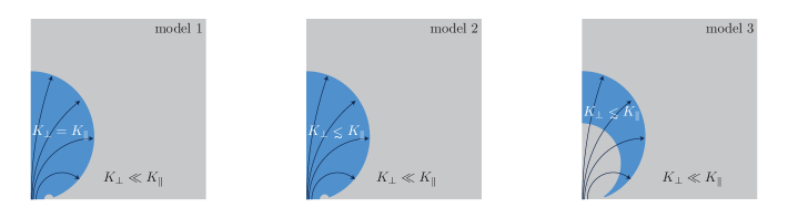
Figure 4: Schematic overview of the three models. (See text for explanations.)

Table 1: Summary of parameter choices in models 1, 2 and 3.

parameter	model 1		model 2		model 3			comment
	inside	halo	inside	halo	inside	shell	halo
$K_{uu,0}\,[10^{-7}\,\text{kpc}^{2}\,\text{yr}^{-1}]$	1	0.1	1	0.1	0.1	1	0.1	perpendicular diffusion coefficient
$K_{vv,0}\,[10^{-7}\,\text{kpc}^{2}\,\text{yr}^{-1}]$	1	10	10	100	100	10	100	parallel diffusion coefficient
$D_{pp,0}\,[10^{-7}\,(\text{GeV}/c)^{2}\,\text{yr}^{-1}]$	10	1	10	1	1	10	1	momentum diffusion coefficient
$\delta$	$1/3$		$1/3$		$1/3$			spectral index
$V_{\text{sh}}\,[10^{-7}\,\text{kpc}\,\text{yr}^{-1}]$	$3$		$3$		$3$			shock speed
$r$	$4$		$4$		$4$			compression ratio

2.6.1 Model 1: isotropic diffusion

In the first setup, we consider diffusion inside the bubbles to be isotropic,

$$K_{uu}=K_{vv}=\beta K_{0}\left(\frac{pc}{1\,\text{GeV}}\right)^{\delta}\,,$$ (31)

where $\beta=v_{\text{particle}}/c$, $K_{0,uu}=K_{0,vv}=10^{-7}\,\text{kpc}^{2}\,\text{yr}^{-1}\approx 3\times 10^{28}\,\text{cm}^{2}\,\text{s}^{-1}$ and $\delta=1/3$. This is close to the diffusion coefficient inferred from the boron–to–carbon ratio measured at the solar position, $K_{\text{iso}}(1\,\text{GeV})\simeq 4.1\times 10^{28}\,\text{cm}^{2}\,\text{s}^{-1}$ (Trotta et al. 2011). Outside the bubbles, in the Galactic halo, we adopt $K_{0,uu}=10^{-8}\,\text{kpc}^{2}\,\text{yr}^{-1}\approx 3\times 10^{27}\,\text{cm}^{2}\,\text{s}^{-1}$ and $K_{0,vv}=10^{-6}\,\text{kpc}^{2}\,\text{yr}^{-1}\approx 3\times 10^{29}\,\text{cm}^{2}\,\text{s}^{-1}$, that is diffusion is markedly anisotropic $(\eta=10)$, with particles diffusing faster along the $v$–direction than along the $u$–direction.

As a fiducial value for the momentum diffusion coefficient, we here adopt $D_{pp,0}=10^{-6}(\text{GeV}/c)^{2}\,\text{yr}^{-1}$ inside the bubbles, so an acceleration time

$$t_{\text{sa}}=p^{2}/D_{pp}\simeq 10^{6}\,\text{yr}\,(pc/1\,\text{GeV})^{\delta}\,.$$ (32)

The Alfvén speed $V_{A}\simeq 300\,\text{km}\,\text{s}^{-1}$ can be accommodated by, e.g., $B_{0}\simeq 6\,\mu\text{G}$ and $n_{\text{gas}}\simeq 2\times 10^{-3}\,\text{cm}^{-3}$. Outside the bubbles, we set $D_{pp,0}=10^{-7}(\text{GeV}/c)^{2}\,\text{yr}^{-1}$, in line with the usual scaling.

2.6.2 Model 2: anisotropic diffusion

For the second setup, we consider the possibility that also diffusion inside the bubbles is anisotropic. Specifically, we adopt $K_{uu,0}=K_{\parallel,0}=10^{-7}\,\text{kpc}^{2}\,\text{yr}^{-1}$ and $K_{vv,0}=K_{\parallel,0}=10^{-6}\,\text{kpc}^{2}\,\text{yr}^{-1}$ inside and $K_{uu,0}=K_{\parallel,0}=10^{-8}\,\text{kpc}^{2}\,\text{yr}^{-1}$ and $K_{vv,0}=K_{\parallel,0}=10^{-5}\,\text{kpc}^{2}\,\text{yr}^{-1}$ outside the bubbles. We keep $\delta$ at $1/3$.

We set $D_{pp,0}=10^{-6}(\text{GeV}/c)^{2}\,\text{yr}^{-1}$ inside the bubbles and $D_{pp,0}=10^{-7}(\text{GeV}/c)^{2}\,\text{yr}^{-1}$ outside the bubbles. All the other parameters plus the ISRFs and the $B$–field are as in the first model, cf. Sec. 2.6.1.

2.6.3 Model 3: anisotropic diffusion and turbulent shell

In the presence of a source of turbulence, the assumption of (almost) isotropic diffusion of the first (second) setup can be justified. In the following we assume that the shock itself is generating such turbulence through hydrodynamic (e.g. Raleigh–Taylor or Kelvin–Helmholtz) instabilities. To take into account that this turbulence could be dissipated at large, kiloparsec distances from the shock, we constrain this region to a shell behind the shock and assume strongly anisotropic diffusion in the rest of the bubble volume (c.f. the right panel of Fig. 4). In particular, we choose

$$K_{uu,0}^{\text{inside}} =10^{-8}\,\text{kpc}^{2}\,\text{yr}^{-1}\quad\text{and}\quad K_{vv,0}^{\text{inside}}=10^{-5}\,\text{kpc}^{2}\,\text{yr}^{-1}$$ (33)

$$K_{uu,0}^{\text{shell}} =10^{-7}\,\text{kpc}^{2}\,\text{yr}^{-1}\quad\text{and}\quad K_{vv,0}^{\text{shell}}=10^{-6}\,\text{kpc}^{2}\,\text{yr}^{-1}$$ (34)

$$K_{uu,0}^{\text{halo}} =10^{-8}\,\text{kpc}^{2}\,\text{yr}^{-1}\quad\text{and}\quad K_{vv,0}^{\text{halo}}=10^{-5}\,\text{kpc}^{2}\,\text{yr}^{-1}\,.$$ (35)

This setup has the added benefit that according to quasi–linear theory, the stochastic acceleration rate $D_{pp}/p^{2}$ is also enhanced in a thin shell,

$$D_{pp,0}^{\text{inside}} =\times 10^{-7}(\text{GeV}/c)^{2}\,\text{yr}^{-1}\,,$$ (36)

$$D_{pp,0}^{\text{shell}} =\times 10^{-6}(\text{GeV}/c)^{2}\,\text{yr}^{-1}\,,$$ (37)

$$D_{pp,0}^{\text{halo}} =\times 10^{-7}(\text{GeV}/c)^{2}\,\text{yr}^{-1}\,.$$ (38)

To match the synchrotron emission, we changed $B_{0}$ to $10\,\mu\text{G}$ and $z_{0}$ to $2\,\text{kpc}$, keeping $\rho_{0}=5\,\text{kpc}$.

In Tbl. 1, we have summarised the most important parameters for the three setups.

3 Results

3.1 Model 1: isotropic diffusion

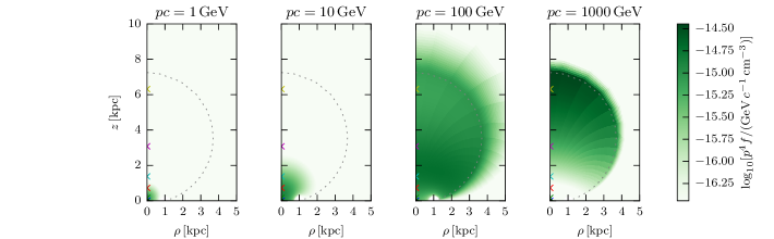
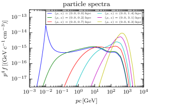
Figure 5: Top: The distribution of electron energy $p^{4}f\sim p^{2}\psi\sim E^{2}n$ at momenta $pc={1,10,10^{2},10^{3}}\,\text{GeV}$ for model 1 at time $t=2.4\times 10^{7}\,\text{yr}$. The black star marks the position of the source where electrons get steadily injected with a momentum $pc=10^{-2}\,\text{GeV}$ and the dashed circle is the shock position at $t=2.4\times 10^{7}\,\text{yr}$. The coloured crosses mark the positions for which the electron spectra are shown in the bottom panel of this figure. Bottom: The spectra $p^{4}f$ at time $t=2.4\times 10^{7}\,\text{yr}$ for the six positions marked by the crosses in the top panel of this figure.

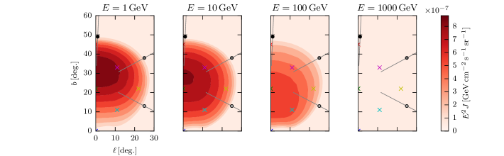
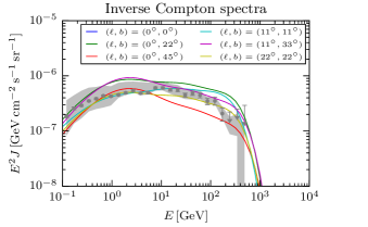
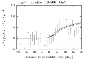
Figure 6: Top: Gamma–ray sky maps at $E=1$, $10$, $10^{2}$ and $10^{3}\,\text{GeV}$ for model 1 (homogeneous bubble, isotropic diffusion) at time $t=2.4\times 10^{7}\,\text{yr}$. The coloured crosses show the directions for which the gamma–ray spectra are shown in the bottom left panel of this figure. The three dots mark the directions where the gradient angular directions are computed and the lines show these directions. The gamma–ray profile along these is shown in the bottom right panel of this figure. Bottom left: Gamma–ray spectra in the directions marked by the crosses in the top panel of this figure. The data points are from Ackermann et al. (2014), showing the statistical errors only. Bottom right: Angular profiles along the directions shown in the top panel of this figure for gamma–rays in the energy range $10-500\,\text{GeV}$. The data points are again from Ackermann et al. (2014).

In the top panels of Fig. 5, we show the distribution of electron energy $p^{4}f\sim p^{2}\psi\sim E^{2}n$ as a function of position at energies $pc=1$, $10$, $10^{2}$ and $10^{3}\,\text{GeV}$ and at time $t=2.4\times 10^{7}\,\text{yr}$. The distribution of electrons at GeV energies is very much confined to the surroundings of the Galactic centre, whereas at $100\,\text{GeV}$ and $1\,\text{TeV}$, the distribution extends up to and beyond the shock. This is due to the fact that high energy electrons have a larger diffusion coefficient and have thus travelled further from the source at the Galactic centre while being further accelerated. At $1\,\text{TeV}$, one can also make out the effect of shock acceleration which is strongest at the top of the bubble where the advection speed is highest, cf. eq. 28. This is leading to a higher electron energy closer to the shock which will help with producing the flat intensity profile in gamma–rays.

The bottom panel of Fig. 5 shows the electron spectra $p^{4}f$ for six positions in the bubbles, marked by the crosses in the top panels. It can be seen that for $z\gtrsim 1\,\text{kpc}$, the electron spectrum is very steep, $f\sim p^{-1}$. The spectral index lies between those predicted for a steady–state situation without ($f\sim p^{0}$) and with ($f\sim p^{-4}$) efficient particle escape (cf., e.g. Stawarz & Petrosian (2008)). The electron energy $p^{4}f$ is peaked at a few hundred GeV. This energy scale is set by competition between stochastic acceleration and radiative energy losses, $t_{\text{sa}}(p_{\text{max}})=t_{\text{cool}}(p_{\text{max}})$. This leads to a pile–up of high–energy electrons just below the maximum energy. At lower energies, the spectrum is much closer to $f\sim p^{-4}$ whereas here, both diffusion and advection play the role of efficient particle escape.

In Fig. 6 we show gamma–ray sky maps at $E=1$, $10$, $10^{2}$ and $10^{3}\,\text{GeV}$ and spectra at six different positions in the bubbles. On average, the spectrum nicely reproduces the measurements by Fermi–LAT (Ackermann et al. 2014). In the bottom right panel, we also show the flux profiles along the gradient directions indicated in the sky maps (upper panels). It can be seen that even in this simple setup, the flux is increasing within $\sim 10^{\circ}$ of the bubble edge, but visually it appears in the sky maps that the bubbles have still edges that are still to soft.

3.2 Model 2: anisotropic diffusion

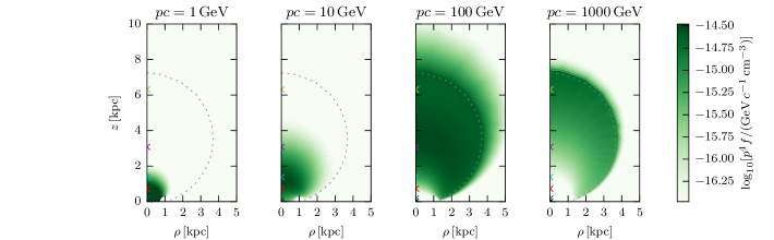
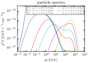
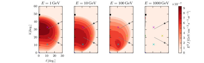
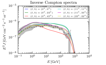
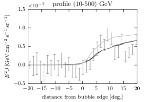
Figure 7: Same as Fig. 5, but for model 2 (homogeneous bubble, anisotropic diffusion) and at time $t=2.4\times 10^{7}\,\text{yr}$.

Figure 8: Same as Fig. 6, but for model 2 (homogeneous bubble, anisotropic diffusion) and at time $t=2.4\times 10^{7}\,\text{yr}$.

Looking at Fig. 8, we see that the morphology of the electron energy ($p^{4}f$) distribution at any one energy has not changed much with respect to the first model, but that the low–energy spectrum is much softer. Most of the electron energy is thus in below–GeV electrons which stay close to the Galactic centre. This can be understood as parallel diffusion is now faster than perpendicular diffusion and therefore fewer particles get transported out into the bubble.

The gamma–ray maps, spectra and profiles, cf. 8, look basically the same, as the high–energy spectrum and morphology are almost unchanged.

3.3 Model 3: anisotropic diffusion and turbulent shell

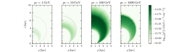
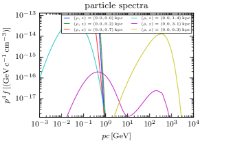
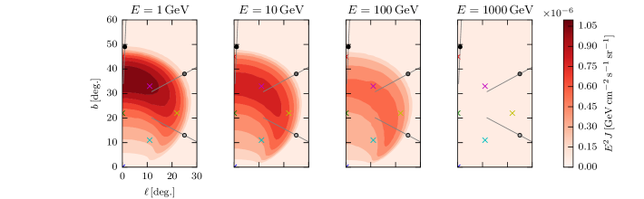
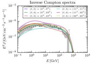
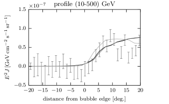
Figure 9: Same as Fig. 5, but for model 3 (bubble with shell, anisotropic diffusion) and at time $t=2.4\times 10^{7}\,\text{yr}$.

Figure 10: Same as Fig. 6, but for model 3 (bubble with shell, anisotropic diffusion) and at time $t=2.4\times 10^{7}\,\text{yr}$.

Fig. 10 shows a marked difference with respect to the other setups: The energy range around $1$ and $10\,\text{GeV}$ is almost devoid of electrons. At lower energies, the spectrum is very soft and peaked. At high energies, the picture is again very similar to models 1 and 2. The morphology at high energies is also different, in that electrons are only present in the shell where stochastic acceleration is efficient.

The spectrum is essentially due to the shell geometry assumed in model 3: We recall that due to the scaling of the momentum diffusion coefficient with turbulence, stochastic acceleration is most efficient in the shell. In addition, perpendicular diffusion is very much suppressed inside the bubbles and in the halo. Therefore, only electrons which were advected into the shell at early times are being stochastically accelerated. Those that did not reach the shell at early times will not be able to catch up with the shell through advection or through diffusion. This constitutes essentially an selection mechanism that limits the number of electron injected into stochastic acceleration.

For the production of gamma–rays, the low energy electrons do not matter. The edges of the bubbles in gamma–rays are now sharper than before, a consequence of high–energy electrons only being present in the shell. Comparing the sky maps at $1$ and $10\,\text{GeV}$, it is apparent that the morphology is spectrally rather uniform, as is in fact observed (Su et al. 2010; Hooper & Slatyer 2013; Ackermann et al. 2014). This is even more obvious from the bottom panel of Fig. 10.

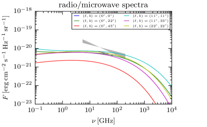
Figure 11: Top: Sky maps of the synchrotron intensity at $0.1$, $1$, $10$ and $100\,\text{GHz}$ for model 3 (anisotropic diffusion and turbulent shell) at time $t=2.4\times 10^{7}\,\text{yr}$, produced by the same electrons shown in Fig. 10. Bottom: Synchrotron spectra for the different directions indicated in the legend and marked by the crosses in the lower panel of Fig. 10. The data points are from Ade et al. (2013) and the bow-tie is from Dobler & Finkbeiner (2008).

Having successfully reproduced the gamma–ray emission, we now ask whether the electrons could also explain the Galactic microwave haze (Dobler & Finkbeiner 2008; Ade et al. 2013). In Fig. 11, we show the synchrotron sky maps at $\nu=\{0.1,1,10,10^{2}\}\,\text{GHz}$ and the synchrotron spectra at various positions in the sky. One can see that the general morphological characteristics of the microwave haze can be reproduced. Note that the enhanced emission around the direction $(\ell,b)=(\pm 15,\pm 10)$ would likely be obscured by conventional diffuse synchrotron emission from the Galaxy.) The synchrotron emission shows a relatively sharp edge in longitude, but decreases rather smoothly beyond $\ell=\pm 20^{\circ}$ as observed (Ade et al. 2013). The computed spectra nicely match the spectral index of $-0.5$ observed at a few tens of GHz, with a hardening below a few GHz; this can explain why no radio counterpart of the microwave haze has been observed (see, however (Carretti et al. 2013)). Note that the data points in Fig. 11 are the average spectrum of the haze and should thus be compared to the average of the model lines.

4 Summary and conclusion

1. We have reviewed the observations of the Fermi bubbles in gamma-rays relevant for the modeling of the emission, transport and acceleration processes with particular focus on their puzzling morphological and spectral properties; namely the constancy of their surface brightness with abrupt edges and relatively uniform hard spectra. We discussed X-ray emission and UV absorption line observations which give (somewhat conflicting) bounds on the outflow velocities in the bubbles and include in our discussion the observations of so-called microwave haze. We reviewed briefly some of the models proposed for production of the bubbles including MHD simulation, jet and Galactic wind models.

2. Our main focus, however, is the acceleration of particles, their transport and emission characteristics with the primary goal of explaining the puzzling morphological and spectral characteristics. We present arguments in favor of leptonic vs. hadronic model and develop kinetic equations to described the acceleration and transport of electrons throughout the bubbles. We include effects of stochastic acceleration by turbulence and those of a low Mach number shock with special attention to momentum and spatial diffusion coefficient in the magnetized medium of the bubble. We also include the effects of energy loss due to inverse Compton and synchrotron processes in a inhomogeneous magnetic and soft photon (CMB, infrared and optical/UV) fields.

3. We present results from three different models with similar characteristics of the (better understood) loss mechanisms but with different assumptions about more uncertain acceleration and other transport characteristics. The first model has isotropic spatial diffusion in the bubble ($\eta=1$) and anisotropic ($K_{uu}\ll K_{vv}$; $\eta=10$) in the halo and higher acceleration rate inside the bubble. This model results in surface brightness distribution not as uniform as observed and can be ruled out. The second model has anisotropic diffusion both inside ($\eta=3.16$) and (even stronger) outside ($\eta=31.6$) in the halo. This model results in a uniform surface brightness but the bubble edge is not as sharp as observed. The third model consists of a relatively thick finite size shell expanding into the halo with mildly anisotropic diffusion in the shell ($\eta=3.16$) but with a much stronger anisotropy inside and outside in the halo ($\eta=31.6$). Acceleration rate is ten times higher in the shell than outside. This model produces a sharper edge and agrees with the observed spectral distribution in gamma-rays and microwave ranges.

4. We conclude that the gamma-ray as well as microwave spectral and morphological features of the Fermi bubbles can be reproduced by the Inverse Compton and synchrotron emission from electrons accelerated by turbulence generated in a mildly supersonic outward flowing shell. This finding is strengthening the scenario where the bubbles are inflated by a wind powered by star formation or star burst activity. Another possibility for inflating the bubbles is a jet from past AGN activity at the center of the galaxy. Whether an in situ acceleration of particles in the jet environment can lead to explanation of observed characteristics of the bubbles as done by our model would require a separate study. If such a future study were to conclude that jet models could not produce the observed properties, it would strengthen the above conclusions based on our current study.