Drift induced by dissipation

Abstract

Active particles have become a subject of intense interest across several disciplines from animal behavior to granular physics. Usually the models of such particles contain an explicit internal driving. Here we propose a model with implicit driving in the sense that the behavior of our particle is fully dissipative at zero temperature but becomes active in the presence of seemingly innocent equilibrium fluctuations. The mechanism of activity is related to the breaking of the gradient structure in the chemo-mechanical coupling. We show that the thermodynamics of such active particles depends crucially on inertia and cannot be correctly captured in the standard Smoluchowski limit. To deal with stall conditions, we generalize the definition of Stokes efficiency, assessing the quality of active force generation. We propose a simple realization of the model in terms of an electric circuit capable of turning fluctuations into a directed current without an explicit source of voltage.

Motile cells, living bacteria, synthetic swimmers and ‘walking’ grains are usually modeled as Active Brownian Particles (ABP) Marchetti et al. [2013], Ramaswamy [2017], Romanzuk et al. [2012], Bechinger et al. [2016]. While it is clear that to achieve persistence, ABPs need to violate fluctuation dissipation theorem and extract energy from the environment, the underlying mechanisms of time reversal symmetry (TRS) breaking at the microscale are known only in few cases Reimann [2002], Nardini et al. [2017]. Moreover, even in those cases, the stochastic thermodynamics of macroscopic directional drift is still replete with ‘hidden effects’ and ‘anomalies’ Celani et al. [2012], Kawaguchi and Nakayama [2013], Mandal et al. [2017], Shankar and Marchetti [2018]. Directionality is usually imposed through the asymmetry of the background potential or the explicit external gradients Bödeker et al. [2010], Friedrich and Jülicher [2007], Selmeczi et al. [2008], Kareiva and Shigesada [1983], Komin et al. [2004], Howse et al. [2007], Paxton et al. [2004], however, it can also arise from velocity-dependent forces Schweitzer et al. [1998], Badoual et al. [2002], Sarracino [2013], Ramaswamy et al. [2003], Manacorda et al. [2014], Vicsek and Zafeiris [2012], Marchetti et al. [2013] allowing the effective friction coefficient to be negative Romanzuk et al. [2012], Ganguly and Chaudhuri [2013], Chaudhuri [2014]. Such forces are then capable of ‘pushing’ the particle and their activity can be interpreted as the presence of ‘anti-dissipation’ at the microscale.

In this Letter we study a more subtle mechanism of directional motility which relies on velocity dependent forces with strictly positive effective viscosity coefficient. Consider, for instance, an inertial dynamics of a particle $m\dot{v}=F+f$, where $m$ is the mass of the particle, $f$ is an external fixed load, $F=-\hat{\gamma}(v)v$ is a frictional force and $\hat{\gamma}\geq 0$ is an effective friction coefficient. At zero temperature this system is clearly dissipative with $fv\geq 0$. However, if one exposes the same particle to an equilibrium thermal reservoir writing dynamics in the form

$$m\dot{v}=F+f+\xi,$$ (1)

where $\langle\xi\rangle=0$ and $\langle\xi(t)\xi(t^{\prime})\rangle\sim\delta(t-t^{\prime})$, it may, for particular choices of the function $\hat{\gamma}(v)$, exhibit ‘anti-dissipative’ behavior with $f\langle v\rangle\leq 0$. In particular, such particle can behave as a Brownian motor with a nonzero drift $\langle v\rangle$ at zero $f$, apparently induced by dissipation. In this Letter we link this phenomenon with non-potential structure of dissipation and strong violation of detailed balance (DB). We address the nontrivial nature of the overdamped limit in such systems and show that the conventional Smoluchowski-type asymptotics fails to describe adequately the underlying energetics. To assess the efficiency of the new motor in the whole range of parameters, we had to go beyond the conventional definitions and view stall conditions as a regime with functional energy consumption.

To motivate the model we consider an underdamped Brownian particle moving in a fluid under the action of viscous friction and thermal noise. Suppose that the translational dynamics of the particle is additionally coupled to a chemical reaction:

$$m\dot{\mathbf{v}} =\mathbf{F}(\mathbf{v},\Delta\mu)+\mathbf{f}+\boldsymbol{\xi}\;$$

$$\dot{\zeta} =A(\mathbf{v},\Delta\mu)$$ (2)

where $\langle\xi_{i}(t)\rangle=0$, and $\langle\xi_{i}(t)\xi_{j}(t^{\prime})\rangle=2\gamma T\delta_{ij}\delta(t-t^{\prime})$, $\gamma$ is the corresponding ‘bare’ viscous coefficient, $T$ is the temperature of the bath (we set Boltzmann constant equal to one) and $A$ is the driving force acting on the reaction coordinate $\zeta$. If chemistry and mechanics are decoupled and the particle is in equilibrium, we have $\mathbf{F}=-\gamma\mathbf{v}$ and $A=\Delta\mu\$ where $\Delta\mu$ is the affinity of the chemical reaction. To break the TRS we assume that the fluxes are related to forces through pseudo-Onsagerian relations Jülicher et al. [1997]

$$\mathbf{F} =-\gamma\mathbf{v}+\lambda\Delta\mu(\mathbf{v}/\|\mathbf{v}\|)\;$$

$$A =-\lambda(\mathbf{v}\cdot\mathbf{m})+\Delta\mu\;$$ (3)

where the coefficient $\lambda$ characterizes chemo-mechanical coupling. The unit vector $\mathbf{m}$ indicates a preferred direction associated, for instance, with an external concentration gradient. Note that in (Drift induced by dissipation, Drift induced by dissipation) the chemical subsystem acts as a feedback controller for the mechanical degrees of freedom.

To ensure analytical transparency, we assume complete separation of time scales in the sense that the reaction is stationary $\dot{\zeta}=0$. Then $\mathbf{F}=-\gamma\big{[}1-\epsilon\,(\mathbf{m}\cdot\mathbf{v})/(\|\mathbf{v}\|)\big{]}\mathbf{v},$ where $\epsilon=\lambda^{2}/\gamma$ is a nondimensional parameter. This form of the friction force highlights the underlying anisotropy in dissipation. A helpful biological reference for this scenario is bacterial flagella whose efficiency for self-propulsion crucially depends on the fact that tangential and normal resistance coefficients are different Lauga and Powers [2009].

Assume now that the vector field $\mathbf{m}$ is constant and homogeneous and let us limit our analysis to one dimension. Then we recover our scalar model (1) with $\hat{\gamma}(v)=\gamma[1+\epsilon\,\text{sgn}(v)],$ where $\text{sgn}(x)$ is the sign function, see also Gidoni et al. [2014]. Note that $\hat{\gamma}(v)\neq\hat{\gamma}(-v)$ and therefore this model violates TRS even when the system is purely dissipative (for $|\epsilon|<1$). If we write $F(v)=-\gamma v+g(v)$, where $g(v)$ is the non-linear contribution to friction, a broken TRS implies that $g(v)\neq-g(-v)$, which is, for instance, in stark contrast with the paradigmatic Rayleigh-Helmholtz model of ABP where always $g(v)=-g(-v)$  Badoual et al. [2002]

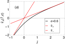
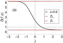
Figure 1: Stationary response of the system (5) at $\epsilon=0.6$: (a) drift velocity (b) diffusion coefficient.

To clarify the difference between these two classes of models, assume that $F=-\gamma v+\varepsilon g(v)$, where $g(v)$ is arbitrary and $\varepsilon>0$ is a small parameter. Assume for generality that the system is also perturbed spatially so that $m\dot{v}=-\gamma v+\varepsilon(g(v)+U^{\prime}(x))+f+\xi$, where $v=\dot{x}$.

We begin by writing the Kramers equation for this system, $\partial_{t}\,P=-\nabla\cdot\mathbf{J}$, where where $\mathbf{q}=(x,v)$, $P(\mathbf{q},t)$ is the probability density and $\mathbf{J}=(J_{x},J_{v})$ is the probability current which can be split in a reversible and a dissipative parts, $\mathbf{J}=\mathbf{J}_{\text{r}}+\mathbf{J}_{\text{d}}$ Risken [1989], with $\mathbf{J}_{\text{r}}=(v\,P,\varepsilon\,m^{-1}[g_{e}(v)-U^{\prime}(x)]P)$, and $\mathbf{J}_{\text{d}}=(0,m^{-1}[\varepsilon g_{o}(v)-\gamma v]P-\gamma Tm^{-2}\partial_{v}P)$ Kwon et al. [2016], Chaudhuri [2016]. Here we distinguished between the even and the odd contributions to the nonlinear force by defining $g_{e,o}=(g(v)\pm g(-v))/2$.

For the DB condition to be satisfied, we must have $\mathbf{J}_{\text{d}}=0$, which means that $\partial_{v}\ln P_{s}=(m/\gamma T)[\varepsilon g_{o}(v)-\gamma v]$, where $P_{s}(v,x)$ is the stationary distribution. This implies that $P_{s}$ must factorize into the product of a velocity-dependent and position-dependent functions. In the stationary state we must also have $\nabla\cdot\mathbf{\mathbf{J}}_{\text{r}}=0$ or

$$\partial_{x}\ln P_{s}-\frac{\varepsilon}{T}U^{\prime}=\frac{\varepsilon}{T}\bigg{[}g_{e}-\frac{T\partial_{v}g_{e}}{m\,v}\bigg{]}+\frac{\varepsilon^{2}g_{o}}{\gamma\,vT}(g_{e}-U^{\prime}).$$ (4)

Since the r.h.s. of (4) cannot depend on $v$ due to the factorization mentioned above, one must have $g_{e,o}=0$. Moreover, we see from (4) that for systems with $g_{e}=0$ but $g_{o}\neq 0$ (Rayleigh-Helmholtz model), the DB condition holds to first order and breaks only at $O(\varepsilon^{2})$ (i.e., only in presence of a coupling with an external potential Sarracino [2013], Manacorda et al. [2014]). Instead, when $g_{e}\neq 0$ but $g_{o}=0$, the DB breaks already at the first order in $\varepsilon$ and without a need for external interactions. It is then clear that the degree of non-equilibrium in systems with $g_{e}\neq 0$ is fundamentally stronger than in systems with $g_{o}\neq 0$.

To illustrate the behavior of a system with $g_{e}\neq 0$ we make the simplest assumption $g(v)=\epsilon\gamma\text{sgn}(v)\,v$, which implies, in particular, that $g_{o}=0$ . We can then drop the irrelevant potential $U(x)$ and, using dimensionless variables $\tilde{v}=v\sqrt{m/T}$, $\tilde{t}=t\gamma/m$, and $\tilde{f}=(f/\gamma)\sqrt{m/T}$, write the dynamic equation in the form

$$\dot{\tilde{v}}=-[1+\epsilon\text{sgn}(\tilde{v})]\tilde{v}+\tilde{f}+\tilde{\xi},$$ (5)

where now $\langle\tilde{\xi}(\tilde{t})\tilde{\xi}(\tilde{t}^{\prime})\rangle=2\delta(\tilde{t}-\tilde{t}^{\prime})$.

The $\tilde{f}$ dependence of the steady-state drift velocity $\tilde{v}_{s}=\langle\tilde{v}\rangle$ can be written explicitly   and the typical $\tilde{v}_{s}(f)$ curve, at $0<\epsilon<1$, is shown in Fig.1a. In addition to two purely dissipative regimes $\tilde{v}_{\pm}(f)=\tilde{f}/(1\pm\epsilon)$ reached at $\tilde{f}\rightarrow\pm\infty$ the system also exhibits ’anti-dissipative’ behavior at small forces when the particle can carry cargo (to the left, as long as $\epsilon>0$). A simple expression can be obtained for $f=0$ where the velocity of active drift takes its maximum value

$$\tilde{v}_{s}^{\text{m}}(\epsilon)=\sqrt{\frac{2}{\pi}}\frac{\sqrt{1-\epsilon}-\sqrt{1+\epsilon}}{\sqrt{1-\epsilon^{2}}}<0.$$ (6)

At $\epsilon\rightarrow 0$, we obtain $-\tilde{v}_{s}^{\text{m}}\sim\epsilon$ or, in dimensional variables, $-v_{s}^{\text{m}}\sim\epsilon\sqrt{T/m}$. In the presence of cargo, the same scaling can be shown for the active part of the drift $v_{s}^{\text{a}}=v_{s}-f/\gamma$, so that again $-v_{s}^{\text{a}}\sim\epsilon\sqrt{T/m}$ for small $\epsilon$. This is a hint that in the overdamped regime the active behavior emerges only in the limit when $\epsilon\sim\sqrt{m}$.

The simplicity of the model allows one also to semi-analytically compute the force dependent effective diffusion coefficient $\tilde{D}=\lim_{\tilde{t}\rightarrow\infty}\langle\tilde{x}^{2}(\tilde{t})\rangle-\langle\tilde{x}(\tilde{t})\rangle^{2}/(2\tilde{t}),$ see Note [1] and Fig. 1. The purely dissipative, large force limits are again different $\tilde{D}_{\pm}=1/(1\pm\epsilon)^{2}$, because the limiting systems can be viewed as equilibrated with reservoirs having different temperatures $\tilde{T}_{\pm}=1/(1\pm\epsilon)$, and viscosities $\tilde{\gamma}_{\pm}=1\pm\epsilon$, so that $\tilde{\gamma}_{+}\tilde{T}_{+}=\tilde{\gamma}_{-}\tilde{T}_{-}\equiv 1$ and $\tilde{D}_{\pm}=\tilde{T}_{\pm}/\tilde{\gamma}_{\pm}$. This observation suggests rewriting our evolution equation (5) in the form

$$\dot{\tilde{v}}=\begin{cases}-\tilde{\gamma}_{-}\tilde{v}+\tilde{f}+\sqrt{2\tilde{\gamma}_{-}\tilde{T}_{-}}\xi_{-}\;\;\;\tilde{v}<0,\\ -\tilde{\gamma}_{+}\tilde{v}+\tilde{f}+\sqrt{2\tilde{\gamma}_{+}\tilde{T}_{+}}\xi_{+}\;\;\;\tilde{v}>0,\end{cases}$$ (7)

with $\langle\xi_{i}(\tilde{t})\xi_{j}(\tilde{t}^{\prime})\rangle=\delta_{ij}\delta(\tilde{t}-\tilde{t}^{\prime})$ and $i,j=\pm$. This stresses the fact that the activity in this system can be interpreted by the exposure of the particle to two reservoirs with different temperatures $\tilde{T}_{\pm}$. Furthermore, such a representation in terms of two Ornstein-Uhlenbeck processes makes explicit the fact that there are two intrinsic inertial time scales, $\tau_{\pm}=m\gamma^{-1}_{\pm}$ (in dimensionful units).

Note that at $\epsilon\to 1$ the temperature of the ‘hot reservoir’ $\tilde{T}_{-}$ diverges and the velocity dynamics becomes Brownian for $\tilde{v}<0$. As a result both the average drift velocity and the recrossing time (from negative to positive velocity) diverge and the dynamics becomes critical exhibiting anomalous unidirectional persistence. At large times one can expect excursions into the preferred direction to dominate implying that $\langle\tilde{x}\rangle\sim-\tilde{t}^{3/2}$, and $\tilde{D}\sim\tilde{t}^{2}$; the associated transients are illustrated in Fig. 2.

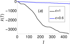
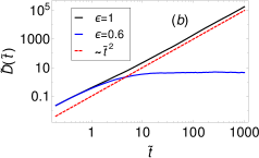
Figure 2: Critical dynamics of a free active particle at $\epsilon=1$: (a) generated stochastic trajectory (black solid line) versus a stochastic trajectory in the case $\epsilon=0.6$; (b) finite time diffusion coefficient.

Observe next that in the double limit $\epsilon\to 0,m\to 0$, with $\epsilon=-v_{s}^{*}\sqrt{\pi m/2T}$, when the active drift velocity has a finite limit, $v_{s}^{\text{a}}\to v_{s}^{*}$, the (dimensional) active diffusion coefficient $D^{a}=D-T/\gamma$ disappears with the scaling $D^{a}\sim\epsilon T/\gamma$. The limiting overdamped dynamics, rigorously justified in Note [1], takes the form

$$\dot{x}=\frac{f}{\gamma}+v_{s}^{*}+\sqrt{\frac{2T}{\gamma}}\xi.$$ (8)

which is often postulated in phenomenological models of ABP, e.g. Golubeva et al. [2012]. Note, however, that the effective model (8), being only a weak limit of the original model (5), only reproduces trajectories faithfully while misrepresenting the structure of velocity fluctuations which are of order $\sim\sqrt{T/m}$ by equipartition. This leads to the appearance of the ‘hidden’ terms in the stochastic thermodynamics of such systems, e.g. Murashita and Esposito [2016], Shankar and Marchetti [2018].

To elucidate this issue we now reintroduce dimensional variables and consider the energetics of a slightly more general model than (5):

$$m\dot{v}=-\gamma v+g_{e}+f+\xi,$$ (9)

where the even function $g_{e}(v)$ is arbitrary. The energy balance along a particular trajectory of duration $\tau$ can be derived by multiplying (9) by $v$ and integrating over time. It reads $\mathcal{E}_{\tau}=\mathcal{U}_{\tau}^{a}-\mathcal{W}_{\tau}-\mathcal{Q}_{\tau}$. Here $\mathcal{E}_{\tau}=(m/2)[v^{2}(\tau)-v^{2}(0)]$ is the change in kinetic energy of the particle, $\mathcal{U}_{\tau}^{a}=\int_{0}^{\tau}dtvg_{e}(v)$ is the active work performed on the particle, $\mathcal{W}_{\tau}=-f\int_{0}^{\tau}dtv$ is the work against the load, and $\mathcal{Q}_{\tau}=\int_{0}^{\tau}dtv(\gamma v-\xi)$ is the released heat Sekimoto [2010]. The stochastic entropy production can be split into a part associated with the system (particle) and another part associated with the reservoir: $\mathcal{S}_{\tau}=\mathcal{S}_{\tau}^{s}+\mathcal{S}_{\tau}^{r}$ Seifert [2012], Note [1]. Here $\mathcal{S}_{\tau}^{s}=\ln[\rho_{0}(v(0))/\rho_{\tau}(v(\tau))]$ is the change of the stochastic Shannon entropy of the particle, whose velocity at time $\tau$ is distributed with the probability density $\rho_{\tau}(v)$, and $\mathcal{S}_{\tau}^{r}=\mathcal{Q}_{\tau}/T-\mathcal{S}_{\tau}^{a}$. The quantity $\mathcal{S}_{\tau}^{a}=m^{-1}\int_{0}^{\tau}dt\partial_{v}f^{\text{nl}}_{e}(v)$ can be interpreted as a leftover of the information exchange between the system and the controller after eliminating the controller degrees of freedom Kim and Qian [2007], *Vel-feedback, Munakata and Rosinberg [2012], *Munakata2, *Munakata3, Horowitz and Sandberg [2014], Chaudhuri [2014, 2016], Marconi et al. [2017], Puglisi and Marini Bettolo Marconi [2017], Mandal et al. [2017], Lee et al. [2013], Kwon et al. [2016], Bandopadhyay et al. [2015]. To compute the total entropy production we used the standard representation $\mathcal{S}_{\tau}=\ln(\mathcal{P}[v]/\hat{\mathcal{P}}[\hat{v}])$ Seifert [2012], where $\mathcal{P}[v]$ is the path probability of the trajectory $v$, while $\hat{\mathcal{P}}[\hat{v}]$ is the probability for the time-reversed trajectory $\hat{v}$ .

The conventional forms of the first and second laws of thermodynamics can be obtained if we average the above expressions over the ensemble of possible trajectories and take time derivatives. Denote by italic capital letters such averages and assume that the system is in a stationary state with $\dot{E}=0$ and $\dot{S}^{s}=0$, where for instance $\dot{E}=(d/d\tau)\langle\mathcal{E}_{\tau}\rangle$. Then we can write:

$$\dot{U}^{\text{a}}-\dot{W}-\dot{Q}=0,\,\,\,\,\dot{S}=\dot{Q}/T-\dot{S}^{\text{a}}=\frac{m^{2}}{\gamma T}\int\frac{J_{d}^{2}(v)}{\rho_{s}(v)}dv\geq 0,$$ (10)

where $J_{d}(v)=-m^{-1}[\gamma v+(\gamma T\,m^{-1})\partial_{v}]\rho_{s}(v)$ denotes, as before, the dissipative part of the stationary current Note [1].

The main shortcoming of the limiting model (8) is that it underestimates entropy production. Indeed, for the overdamped dynamics (8), the stationary entropy production rate can be written as

$$\dot{S}_{\text{od}}=\frac{1}{\gamma T}(f+\gamma v_{s}^{*})^{2}\geq 0.$$ (11)

It is clearly associated with passive dissipation described in (10) by the term $\dot{Q}/T$. In stall conditions this expression vanishes because (8) does not see the fast dynamics at the microscale. If we now compute the entropy production for the full model (5) and go to the limit $m\to 0$ with $\epsilon\sim\sqrt{m}$ we obtain Note [1]

$$\dot{S}=\dot{S}_{\text{od}}+\bigg{(}\frac{\pi}{2}-1\bigg{)}\frac{\gamma(v_{s}^{*})^{2}}{T}\geq 0,$$ (12)

where the second term constitutes the ‘hidden’ entropy production.

To assess the efficiency of our ABP it is natural to first introduce the injection rate of the Helmholtz free energy $\dot{F}^{\text{a}}=\dot{U}^{\text{a}}-T\dot{S}^{\text{a}}$. Then the inequality in (10) can be rewritten as $T\dot{S}=\dot{F}^{\text{a}}-\dot{W}\geq 0,$ which suggests the following definition of the thermodynamic efficiency, $\eta_{T}=\dot{W}/\dot{F}^{\text{a}}\equiv\dot{W}/(T\dot{S}+\dot{W})\leq 1$ Cao and Feito [2009], Recho et al. [2014]. This definition, however, neither accounts for the capacity of a motor to self-propel at zero force, nor for its ability to generate force in stall conditions: in both limits the machine works (either by achieving persistent unidirectional displacement or equally persistent localization) with apparently zero efficiency. A known way to resolve the first of these issues is to consider the Stokes efficiency Wang and Oster [2002], $\eta_{S}=(\dot{W}+\gamma v_{s}^{2})/\dot{F}^{\text{a}}$, which still vanishes in stall conditions.

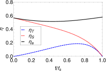
Figure 3: Typical force dependence of the thermodynamic efficiency $\eta_{T}$, Stokes efficiency $\eta_{S}$ and the new efficiency $\eta_{\text{a}}$ for the model (5) with $\epsilon=0.9$. The force $f$ is normalized by the stall value (denoted by $f_{s}$).

To fix this problem we observe that the (squared) total active force generated by the controller is $\langle g_{e}(v)^{2}\rangle$, while only an amount $\langle g_{e}(v)\rangle^{2}$ is useful. The efficiency of active force generation can then be quantified as $\eta_{\text{a}}=\langle g_{e}(v)\rangle^{2}/\langle g_{e}(v)^{2}\rangle$ or in thermodynamic terms Note [1]

$$\eta_{\text{a}}=\dot{W}^{\text{a}}/\dot{G}^{\text{a}}.$$ (13)

Here $\dot{W}^{\text{a}}=\gamma(v_{s}^{\text{a}})^{2}$ is now interpreted as useful power, where $v_{s}^{\text{a}}=v_{s}-f/\gamma$ is the active velocity gain introduced previously; observe that it is finite in both zero force and zero velocity limits. The consumed power is naturally measured by the rate of injected Gibbs free energy $\dot{G}^{\text{a}}=\dot{F}^{\text{a}}-fv_{s}^{\text{a}}\geq\dot{F}^{\text{a}}$ which is also natural given that the system is performing work against the load. The typical behavior of thermodynamic, Stokes, and force generation (13) efficiencies is illustrated for our model in Fig. 3. Note that the definition (13) is different from the recently introduced notion of chemical efficiency Baerts et al. [2017] which may attain negative values and does not reduce to the Stokes efficiency $\eta_{S}$ in the absence of load.

We now briefly discuss a simple experimentally testable realization of the system (5) in the form of an electric circuit where an active current may appear in the absence of directed voltage, see Fig. 4. The ‘fluctuator’ part of the circuit contains an electric resistance $R_{f}$ and an ideal inductance $L$. We assume the ‘fluctuator’ to be in thermal contact with a bath at temperature $T_{f}$. The ‘rectifier’ is made of two parallel branches, each containing a resistor $R_{i}$ and an ideal diode $D_{i}$ in series ($i=1,2$), and is in thermal contact with another bath with temperature $T_{r}<<T_{f}$. This inequality is essential to ensure that electrical fluctuations are basically produced only in resistor $R_{f}$ while the ‘rectifier’ plays the role of the active mechanism alternating the effective resistance depending on the direction of the current in the ‘fluctuator’.

Standard circuit analysis leads to the following equation for the global current $I$  Note [1]:

$$L\dot{I}=-R_{e}(1+\epsilon\text{sgn}(I))I+\sqrt{2R_{e}T_{e}}\xi,$$ (14)

where the effective parameters are $R_{e}=R_{f}+(R_{1}+R_{2})/2$, $T_{e}=2R_{f}T_{f}/(2R_{f}+R_{1}+R_{2})$ and $\epsilon=(R_{2}-R_{1})/(2R_{f}+R_{1}+R_{2})$. We assumed that the current is positive when flowing clockwise around the circuit. As the analogy between (5) in the absence of load, and (14) is complete, the circuit in Fig. 4 should be able to generate a directed current by rectifying thermal fluctuations; the ‘activity’ is then ensured by the device maintaining the temperature difference between the ‘fluctuator’ and the ‘rectifier’.

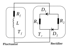
Figure 4: Electric circuit imitating the behavior of the system (5) when $T_{r}<<T_{f}$.

To conclude, we presented a model of an active particle exploiting ’strong’ mechanism of TRS breaking. This model appears naturally if one makes the simplest pseudo-linear assumptions about the chemo-mechanical coupling of the vectorial (friction) and the scalar (reaction) processes which breaks the potentiality of the dissipative potential. While the realistic chemomecanical coupling is probably more complex, for instance quadratic, as in the case of KPZ equation Kardar et al. [1986] or the active model B Wittkowski et al. [2014], the main idea of the breaking the TRS symmetry through non-gradient dissipation can be already captured by our semi-analytical model. An important result of our analysis is that in systems with non-Maxwellian velocity distribution and persistence, the Smoluchowski limit aimed at capturing trajectories can grossly underestimate the associated dissipation, giving a misleading picture of the fluctuation rectification process.

Acknowledgments. The authors thank J.F. Joanny for helpful discussions. R.G.G. acknowledges financial support from the Grant ANR-10-LBX-0038 which is a part of the IDEX PSL ( ANR-10-IDEX-0001-02 PSL). L. T. was supported by the Grants ANR-10-IDEX-0 0 01-02 PSL and ANR-17-CE08-0 047-02.

References

- Marchetti et al. [2013] M. C. Marchetti, J. F. Joanny, S. Ramaswamy, T. B. Liverpool, J. Prost, M. Rao, and R. A. Simha, Rev. Mod. Phys. 85, 1143 (2013).
- Ramaswamy [2017] S. Ramaswamy, J. Stat. Mech. , P054002 (2017).
- Romanzuk et al. [2012] P. Romanzuk, M. Bär, W. Ebeling, B. Lindner, and L. Schimansky-Geier, Eur. Phys. J. Special Topics 202, 1 (2012).
- Bechinger et al. [2016] C. Bechinger, R. Di Leonardo, H. Löwen, C. Reichhardt, G. Volpe, and G. Volpe, Rev. Mod. Phys. 88, 045006 (2016).
- Reimann [2002] P. Reimann, Phys. Rep. 361, 57 (2002).
- Nardini et al. [2017] C. Nardini, E. Fodor, E. Tjhung, F. van Wijland, J. Tailleur, and M. E. Cates, Phys. Rev. X 7, 021007 (2017).
- Celani et al. [2012] A. Celani, S. Bo, R. Eichhorn, and E. Aurell, Phys. Rev. Lett. 109, 260603 (2012).
- Kawaguchi and Nakayama [2013] K. Kawaguchi and Y. Nakayama, Phys. Rev. E 88, 022147 (2013).
- Mandal et al. [2017] D. Mandal, K. Klymko, and M. R. DeWeese, Phys. Rev. Lett. 119, 258001 (2017).
- Shankar and Marchetti [2018] S. Shankar and M. C. Marchetti, “Hidden entropy production and work fluctuations in an active gas,” (2018), arXiv preprint arXiv:1804.03099.
- Bödeker et al. [2010] H. Bödeker, C. Beta, T. Frank, and E. Bodenschatz, Eur. Phys. Lett. 90, 28005 (2010).
- Friedrich and Jülicher [2007] B. M. Friedrich and F. Jülicher, Proc. Natl. Acad. Sci. 104, 13256 (2007).
- Selmeczi et al. [2008] D. Selmeczi, L. Li, L. Pedersen, S. Nrrelykke, P. Hagedorn, S. Mosler, N. Larsen, E. Cox, and H. Flyvbjerg, Eur. Phys. J. Special Topics 157, 1 (2008).
- Kareiva and Shigesada [1983] P. Kareiva and N. Shigesada, Oecologia 56, 234 (1983).
- Komin et al. [2004] N. Komin, U. Erdmann, and L. Schimansky-Geier, Fluct. Noise Lett. 4, L151 (2004).
- Howse et al. [2007] J. R. Howse, R. A. Jones, A. J. Ryan, T. Gough, R. Vafabakhsh, and R. Golestanian, Phys. Rev. Lett. 99, 048102 (2007).
- Paxton et al. [2004] W. F. Paxton, K. C. Kistler, C. C. Olmeda, A. Sen, S. K. St. Angelo, Y. Cao, T. E. Mallouk, P. E. Lammert, and V. H. Crespi, J. Amer. Chem. Soc. 126, 13424 (2004).
- Schweitzer et al. [1998] F. Schweitzer, W. Ebeling, and B. Tilch, Phys. Rev. Lett. 80, 5044 (1998).
- Badoual et al. [2002] M. Badoual, F. Jülicher, and J. Prost, Proc. Natl. Acad. Sci. 99, 6696 (2002).
- Sarracino [2013] A. Sarracino, Phys. Rev. E 88, 052124 (2013).
- Ramaswamy et al. [2003] S. Ramaswamy, R. A. Simha, and J. Toner, Europhys. Lett. 62, 196 (2003).
- Manacorda et al. [2014] A. Manacorda, A. Puglisi, and A. Sarracino, Commun. Theor. Phys. 62, 505 (2014).
- Vicsek and Zafeiris [2012] T. Vicsek and A. Zafeiris, Phys. Rep. 517, 71 (2012).
- Ganguly and Chaudhuri [2013] C. Ganguly and D. Chaudhuri, Phys. Rev. E 88, 032102 (2013).
- Chaudhuri [2014] D. Chaudhuri, Phys. Rev. E 90, 022131 (2014).
- Jülicher et al. [1997] F. Jülicher, A. Ajdari, and J. Prost, Rev. Mod. Phys. 69, 1269 (1997).
- Lauga and Powers [2009] E. Lauga and T. R. Powers, Rep. Prog. Phys. 72, 096601 (2009).
- Gidoni et al. [2014] P. Gidoni, G. Noselli, and A. DeSimone, Int. J. Non Linear Mech. 61, 65 (2014).
- Risken [1989] H. Risken, The Fokker-Planck Equation: Methods of Solution and Applications, 2nd ed. (Berlin: Springer-Verlag, 1989).
- Kwon et al. [2016] C. Kwon, J. Yeo, H. K. Lee, and H. Park, J. Korean Phys. Soc. 68, 633 (2016).
- Chaudhuri [2016] D. Chaudhuri, Phys. Rev. E 94, 032603 (2016).
- Note [1] See Supplemental Material at [URL will be inserted by publisher].
- Golubeva et al. [2012] N. Golubeva, A. Imparato, and L. Peliti, Europhys. Lett. 97, 60005 (2012).
- Murashita and Esposito [2016] Y. Murashita and M. Esposito, Phys. Rev. E 94, 062148 (2016).
- Sekimoto [2010] K. Sekimoto, Stochastic energetics, 799 No. 1 (Springer-Verlag Berlin Heidelberg, 2010).
- Seifert [2012] U. Seifert, Rep. Prog. Phys. 75, 126001 (2012).
- Kim and Qian [2007] K. H. Kim and H. Qian, Phys. Rev. E 75, 022102 (2007).
- Kim and Qian [2004] K. H. Kim and H. Qian, Phys. Rev. Lett. 93, 120602 (2004).
- Munakata and Rosinberg [2012] T. Munakata and M. L. Rosinberg, J. Stat. Mech , P05010 (2012).
- Munakata and Rosinberg [2013] T. Munakata and M. L. Rosinberg, J. Stat. Mech. , P06014 (2013).
- Munakata and Rosinberg [2014] T. Munakata and M. L. Rosinberg, Phys. Rev. Lett. 112, 180601 (2014).
- Horowitz and Sandberg [2014] J. M. Horowitz and H. Sandberg, New J. Phys. 16, 125007 (2014).
- Marconi et al. [2017] U. M. B. Marconi, A. Puglisi, and C. Maggi, Sci. Rep. 7, 46496 (2017).
- Puglisi and Marini Bettolo Marconi [2017] A. Puglisi and U. Marini Bettolo Marconi, Entropy 19 (2017), 10.3390/e19070356.
- Lee et al. [2013] H. K. Lee, C. Kwon, and H. Park, Phys. Rev. Lett. 110, 050602 (2013).
- Bandopadhyay et al. [2015] S. Bandopadhyay, D. Chaudhuri, and A. M. Jayannavar, Phys. Rev. E 92, 032143 (2015).
- Note [2] In contrast to Refs. Marconi et al. [2017], Puglisi and Marini Bettolo Marconi [2017], Mandal et al. [2017], where activity was modeled by colored noise, and to feedback cooling systems, e.g., Refs. Kim and Qian [2007], *Vel-feedback, Munakata and Rosinberg [2012], *Munakata2, *Munakata3, here we do not need to rely on special assumptions about the time-reversed dynamics, see Note [1] for details.
- Cao and Feito [2009] F. J. Cao and M. Feito, Phys. Rev. E 79, 041118 (2009).
- Recho et al. [2014] P. Recho, J.-F. Joanny, and L. Truskinovsky, Phys. Rev. Lett. 112, 218101 (2014).
- Wang and Oster [2002] H. Wang and G. Oster, Europhys. Lett. 57, 134 (2002).
- Baerts et al. [2017] P. Baerts, C. Maes, J. Pešek, and H. Ramon, “Tension and chemical efficiency of myosin-ii motors,” (2017), arXiv preprint arXiv:1708.07454.
- Kardar et al. [1986] M. Kardar, G. Parisi, and Y.-C. Zhang, Phys. Rev. Lett. 56, 889 (1986).
- Wittkowski et al. [2014] R. Wittkowski, A. Tiribocchi, J. Stenhammar, R. J. Allen, D. Marenduzzo, and M. E. Cates, Nat. Commun. 5, 4351 (2014).