NuSTAR observations of Mrk 766: distinguishing reflection from absorption

Abstract

We present two new NuSTAR observations of the narrow line Seyfert 1 (NLS1) galaxy Mrk 766 and give constraints on the two scenarios previously proposed to explain its spectrum and that of other NLS1s: relativistic reflection and partial covering. The NuSTAR spectra show a strong hard ($>15$ keV) X-ray excess, while simultaneous soft X-ray coverage of one of the observations provided by XMM-Newton constrains the ionised absorption in the source. The pure reflection model requires a black hole of high spin ($a>0.92$) viewed at a moderate inclination ($i=46_{-4}^{+1}\,{}^{\circ}$). The pure partial covering model requires extreme parameters: the cut-off of the primary continuum is very low ($22_{-5}^{+7}$ keV) in one observation and the intrinsic X-ray emission must provide a large fraction (75%) of the bolometric luminosity. Allowing a hybrid model with both partial covering and reflection provides more reasonable absorption parameters and relaxes the constraints on reflection parameters. The fractional variability reduces around the iron K band and at high energies including the Compton hump, suggesting that the reflected emission is less variable than the continuum.

1 Introduction

A common feature of the X-ray spectra of many non-jetted active galactic nuclei (AGN) is the hard excess, a strong increase in flux above $\sim 15$ keV. This was first detected in stacked spectra from Ginga (Pounds et al., 1990) and measured for individual sources with BeppoSAX (Perola et al., 2002). Prior to the launch of NuSTAR, detailed measurements had only been made in a handful of AGN, using Swift-BAT or the Suzaku PIN detector, which were interpreted either as evidence of Compton thick absorption (Risaliti et al., 2009; Turner et al., 2009) or the Compton hump of reflected emission (Walton et al., 2010). X-ray reflection (Lightman & White, 1988; George & Fabian, 1991) occurs when the primary X-ray source, known as the corona, illuminates the accretion disc or other relatively cold material such as the torus. This illumination triggers the emission of fluorescent lines at low energies and is scattered into a ‘Compton hump’ at high energies. When the reflection spectrum originates from the parts of the accretion disc close to the innermost stable circular orbit (ISCO) of the black hole, the narrow features are blurred out by relativistic effects (Fabian et al., 1989; Laor, 1991).

Since the launch of NuSTAR (Harrison et al., 2013), the Compton hump has been more definitively detected in many AGN (Risaliti et al., 2013; Walton et al., 2014; Marinucci et al., 2014; Brenneman et al., 2014; Parker et al., 2014b; Baloković et al., 2015; Kara et al., 2015). The sensitivity of NuSTAR at high energies means that it can be used to differentiate between reflection and absorption models for the hard excess (e.g. Vasudevan et al., 2014).

One object which has had both these processes proposed to explain its spectrum is Mrk 766. Mrk 766 is a nearby ($z=0.013$) narrow line Seyfert 1 (NLS1) galaxy. NLS1s are thought to be rapidly accreting ($\dot{m}\sim 0.01-1$), relatively low mass (typically $M_{\rm BH}\sim 10^{6}-10^{7}M_{\odot}$) AGN, and are distinguished by narrow optical Balmer lines, weak [O iii] and strong Fe ii emission (see review by Komossa, 2008). In the X-ray band, NLS1s are spectrally soft, and are thus easily detected by low energy instruments. They frequently show complex, rapid variability and non-trivial spectral shapes, so are of great interest for study. The supermassive black hole in the nucleus of Mrk 766 has a mass of 1–6$\times 10^{6}M_{\odot}$ (Bentz et al., 2009, 2010) and the host is a barred spiral galaxy. Spectrally, the evidence for a relativistically-broadened iron line in Mrk 766 is tentative. A broad line was claimed with ASCA by Nandra et al. (1997b). However, later analysis of a more sensitive XMM-Newton spectrum by Pounds et al. (2003) showed that the line profile could instead be described by ionized reflection alone, with no need for relativistic blurring. Based on XMM-Newton and Suzaku observations of Mrk 766, Miller et al. (2007) and Turner et al. (2007) proposed a model where the bulk of the spectral variability is due to variations in multiple complex (partially-covering, ionized) absorbing zones. A recent re-analysis of the archival XMM-Newton data by Liebmann et al. (2014) showed that the spectra and variability could be well described by a composite model, containing both partial-covering absorption and relativistic reflection.

More robust evidence for the presence of relativistic reflection in Mrk 766 comes from the detection of a reverberation lag (Emmanoulopoulos et al., 2011; De Marco et al., 2013), thought to be caused by the time delay induced in the reflected signal due to the light travel time from the corona to the disc. Emmanoulopoulos et al. (2011) found almost identical reverberation lags in Mrk 766 and MCG–6-30-15, the first source in which a broad iron line was discovered (Tanaka et al., 1995). Mrk 766 is included in the sample of objects studied by Emmanoulopoulos et al. (2014), who found that by modelling the time lag spectra they could precisely determine the mass ($M_{\rm BH}=1.6_{-1.2}^{+1.4}\times 10^{6}\,M_{\sun}$) and constrain other physical parameters (e.g. the dimensionless spin, $a>0.56$). The discovery of iron K lags in some sources (e.g. Zoghbi et al., 2012; Kara et al., 2013, 2016), which have so far only been explained by invoking relativistic reflection, have reinforced the interpretation of these high-frequency time lags as originating from reverberation close to the black hole. However, iron K reverberation lags have not yet been detected in Mrk 766 (Kara et al., 2016).

In this paper, we present the results of recent NuSTAR observations of Mrk 766, where we examine the hard X-ray spectrum using the sensitivity and high-energy spectral resolution of NuSTAR to enable us to constrain the different physical models for the hard excess. The observations and methods of data reduction are presented in Section 2; results of the analysis are given in Section 3; these results are discussed in Section 4; and conclusions are made in Section 5.

2 Observations and Data Reduction

Table 1: List of NuSTAR observations of Mrk 766 and associated simultaneous X-ray observations.

Telescope	OBSID	Start time	Observation length/ks
NuSTAR	60101022002	2015-01-24T12:31	90.2
Swift-XRT	00080076002	2015-01-25T00:08	4.9
NuSTAR	60001048002	2015-07-05T22:24	23.6
XMM-EPIC	0763790401	2015-07-05T17:26	28.2

Mrk 766 has been observed twice by NuSTAR: for 90 ks starting on 2015 Jan 24 and for 23 ks starting on 2015 July 5. The first observation had a simultaneous Swift snapshot and the second was taken jointly with XMM-Newton (see Table 1).

The NuSTAR data were reduced using the NuSTAR data analysis software (NuSTARDAS) version 1.4.1, and CALDB version 20140414. We extracted cleaned event files using the nupipeline command, and spectral products using the nuproducts command, using 80 arcsec radius circular extraction regions for both source and background spectra. The background region was selected from a region on the same chip, uncontaminated with source photons or background sources.

The Swift data were reduced using the Swift XRT products generator, using the procedure described in Evans et al. (2009) to extract a spectrum.

The XMM-Newton data, taken in small window mode, were reduced according to the standard guidelines in the XMM-Newton User’s Manual, using the XMM-Newton Science Analysis Software (sas) version 14.0.0 as described in Vasudevan et al. (2013). The task epchain was used to reduce the data from the pn instrument. An annular source region of outer radius 40 arcsec and inner radius 10 arcsec was used to extract a source spectrum to remove mild pileup (detected using the epatplot tool), checking for nearby sources in the extraction region. Circular regions near the source were used to calculate the background. Additionally, the background light curves (between 10 and 12 keV) were inspected for flaring, and a comparison of source and background light curves in the same energy ranges was used to determine the portions of the observation in which the background was sufficiently low compared to the source (4 ks was lost to flaring); the subsequent spectra were generated from the usable portions of the observation. Response matrices and auxiliary files were generated using the tools rmfgen and arfgen.

We use XMM-Newton-RGS data from the new observation and the highest and lowest flux archival observations (OBSIDs: 0304030101, 0304030301). We reduced the data with the standard XMM-Newton pipeline, rgsproc. We use a source region including 95% of the PSF and background from outside 98% of the PSF (xpsfincl=95 and xpsfexcl=98). The two detectors were added for illustrative purposes only using rgscombine.

Spectra from all instruments were grouped to a signal to noise level of 5. Fits were made in ISIS Version 1.6.2-32 (Houck & Denicola, 2000); errors are given at the 90% level. We use the elemental abundances of Wilms et al. (2000) with cross sections from Verner et al. (1996).

3 Results

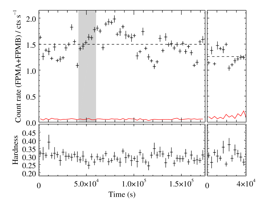
Figure 1: Upper Panels: NuSTAR light curve with 3 ks bins. The gap between panels corresponds to $\sim 6$ months. The background light curve is shown in red, and the time of the Swift XRT exposure by the shaded region. The dashed horizontal lines show the mean flux of each observation. Lower panels: 10–40/3–10 keV hardness ratio.

From the NuSTAR lightcurve (Fig. 1), we determine that no significant long term flux or hardness variability is seen. It is therefore appropriate to fit average spectra of each observation. The Swift X-ray telescope (XRT) snapshot taken during the first NuSTAR observation (shown by the shaded region in Fig. 1) occurred at a flux level close to the average. Therefore, it is likely to be indicative of the average low energy spectrum over the whole observation.

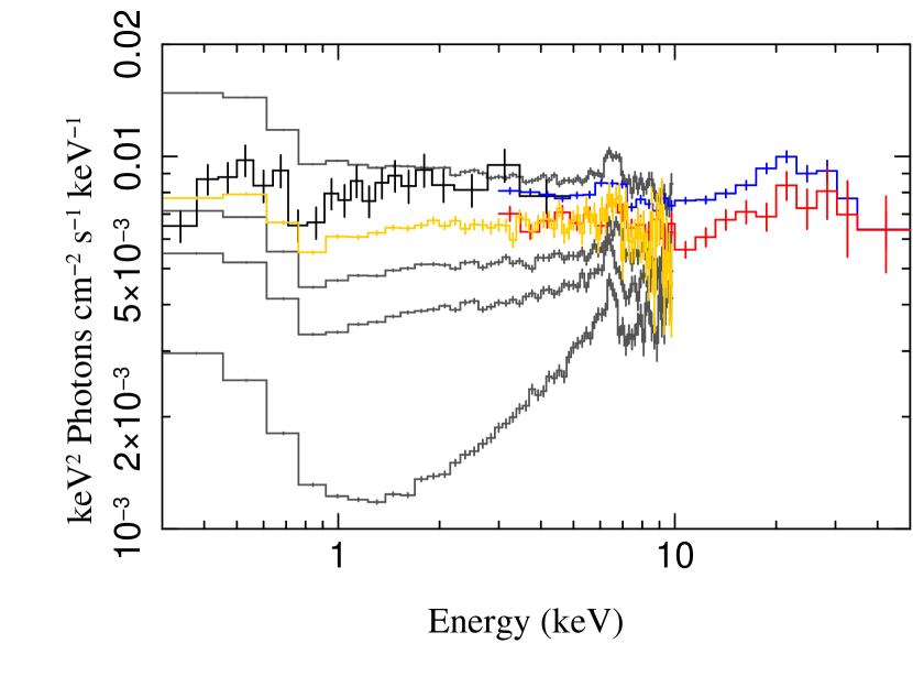
Figure 2: Unfolded fluxes (to a $\Gamma=2$ powerlaw) of the January (NuSTAR: blue, Swift: black) and July (NuSTAR: red, XMM: orange) observations, with a range of previous XMM (grey) observations (OBSIDs 0109141301, 0304030101, 0304030301 and 0304030401, see Miller et al. 2007; Giacchè et al. 2014 for detailed analysis). Spectra have been rebinned for plotting.

We compare the NuSTAR observations with previous observations in Fig. 2. This shows that the new observations are close to the high flux end of the previously observed states of Mrk 766.

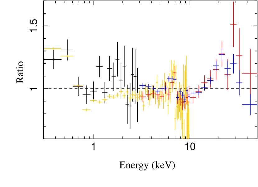
Figure 3: Ratios of each observation to a $\Gamma=2$ powerlaw with Galactic absorption: January Swift (black) and NuSTAR (blue); July XMM-PN (orange) and NuSTAR (red). Spectra have been rebinned for plotting.

We begin our analysis by comparing all data for each of the new observations to a powerlaw with Galactic absorption (modelled with tbnew, Wilms et al. 2000). The residuals to a $\Gamma=2$ powerlaw are shown in Fig. 3. This shows the spectrum is moderately soft, with a soft excess below 0.7 keV with a deficit above, and excesses at $5-7$ keV and $15-40$ keV.

The drop in flux at $\sim 0.7$ keV may be due to warm absorption features such as the OVII edge and the iron unresolved transition array (UTA). The excesses at $5-7$ keV and $15-40$ keV are typical of emission from Fe K and Compton scattering due to reflection, but similar features can be produced by partial covering absorption reducing the flux at other energies. We therefore proceed by fitting detailed models of these processes to the spectra. Since different processes dominate the spectral features in the low and high energy data, we first consider each region separately, before combining these to give a consistent broadband picture.

3.1 High-energy fits – iron line and hard excess

To constrain the iron line and hard excess while minimising the effect of absorption, we initially fit the data above 3 keV. Since the Swift observation has little signal above 3 keV, we fit only the data from NuSTAR and XMM-pn. We fit the two observations separately.

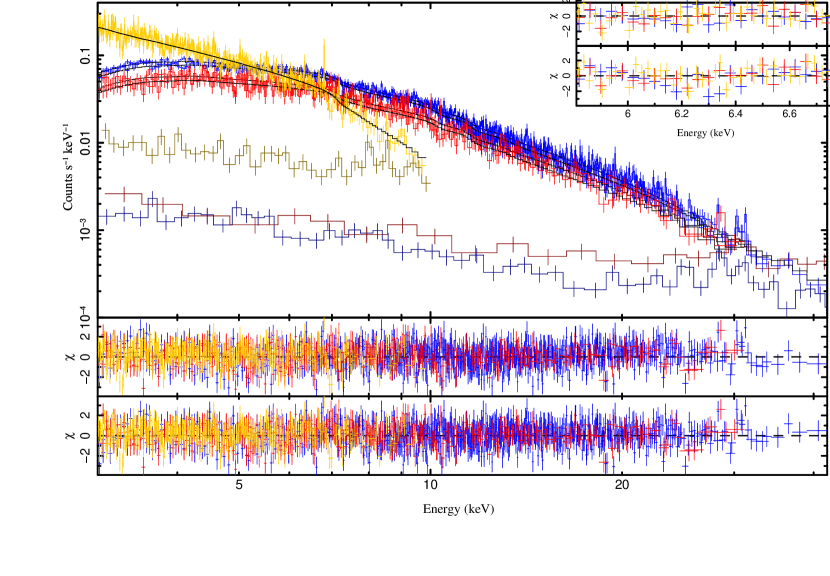
Figure 4: Top panel: fits to NuSTAR and XMM-Newton data above 3 keV (the model shown is of relativistic reflection). XMM-Newton data in orange is simultaneous with the red (dimmer) NuSTAR data; the other NuSTAR observation is shown in blue. Backgrounds are shown in dark orange, red and blue respectively. Middle panel: residuals from relativistic reflection model. Lower panel: residuals from partial covering model. Inset: Residuals for reflection models over $5.8-6.8$ keV. Blurred reflection (upper inset) has smaller residuals around the iron K band than distant neutral reflection (lower inset): over $5.8-6.8$ keV, $\Delta\chi^{2}=18$.

In the reflection case, we find that distant reflection (modelled with pexmon, Magdziarz & Zdziarski 1995; Nandra et al. 2007) is insufficient to model the iron line ($\chi^{2}/{\rm d.o.f.}=1682/1526=1.102$), leaving residuals around the narrow iron line (Fig. 4, inset), which suggest that the iron line is broadened. We test this by replacing the narrow iron line in pexmon with a broadened gaussian (pexrav+zgauss). This gives a significantly better fit, $\Delta\chi^{2}=46$ and $17$ for the Swift/NuSTAR and XMM-Newton/NuSTAR observations repectively. Parameters of fits to this model are shown in Table 2. This shows significant width to the iron line, likely due to the orbital motion of material around the black hole.

Having shown that the iron line is broadened, we fit the spectrum with a reflection model that incorporates self-consistent relativistic blurring of the entire spectrum (relxill, Dauser et al. 2010; García et al. 2014). This provides a reasonably good fit ($\chi^{2}/{\rm d.o.f.}=1607/1518=1.059$). Further, we note that including distant reflection does not provide a significant improvement over relativistic reflection alone ($\Delta\chi^{2}=6$ for 2 additional degrees of freedom) and no physical parameters of the relativistic model change significantly. Hence, we present models including only relativistic reflection (Table 2).

These models show Mrk 766 as a source with slight relativistic blurring viewed at moderate inclination ($i=42\pm 3^{\circ}$ or ${39_{-3}^{+6}}^{\circ}$). Parameters such as the inclination, which are not expected to change within 6 months, are consistent between the two observations. The cut-off of the primary continuum is too high to measure.

It has also been suggested that the spectrum of Mrk 766 can be explained by partial covering absorption of the primary source (Miller et al., 2007; Turner et al., 2007). We model this with a cut-off power-law with a number of partially covering components, using the model zpcfabs. We find that a model with two components ($\chi^{2}/{\rm d.o.f.}=1616/1522=1.062$) provides a similar quality fit to the reflection model. Having only one partial covering component gives a significantly worse fit to the data ($N_{\rm H}\sim 9\times 10^{24}$ cm^-2, $f_{\rm cov}\sim 0.6$, $\chi^{2}/{\rm d.o.f.}=1693/1526=1.110$) and three partial covering components gives insignificant improvement over 2 components ($\Delta\chi^{2}=8$ for 4 degrees of freedom).

The two-component fit requires a component of strong absorption ($N_{\rm H}>5\times 10^{24}$ cm^-2) in each observation and a low energy of the cut-off ($E_{\rm cut}=27_{-9}^{+20}$ keV) in the Swift/NuSTAR observation, which has better high energy statistics due to the longer NuSTAR exposure.

Table 2: Fits to data from each observation above 3 keV. Parameters indicated with * are fixed. $R_{\rm Refl}$ indicates the reflection strength, where $R_{\rm Refl}=1$ gives the reflection from material covering $2\pi$ steradians with an isotropic source.

Parameter	Swift/NuSTAR	XMM-Newton/NuSTAR
Reflection with broad Gaussian iron line
$\Gamma$	$2.46_{-0.08}^{+0.08}$	$2.31\pm 0.12$
$E_{\rm cut}$/keV	$>440$	$>310$
$R_{\rm Refl}$	$3.5_{-0.9}^{+1.0}$	$2.1_{-0.9}^{+1.2}$
Line $E$ /keV	$6.4$*	$6.4$*
Line $\sigma$ /keV	$2.3_{-0.4}^{+0.3}$	$1.4_{-0.7}^{+0.5}$
$\chi^{2}/$d.o.f.	$909.2/806=1.128$	$710.6/718=0.990$
Relativistic reflection
Emissivity Index	$<4$	$>4.3$
$a$	Unconstrained	$<0.44$
$i/^{\circ}$	$42_{-3}^{+3}$	$39_{-3}^{+6}$
$\Gamma$	$2.24_{-0.05}^{+0.09}$	$2.16_{-0.08}^{+0.12}$
$\log(\xi/{\rm erg\,cm\,s^{-1}})$	$1.8_{-0.5}^{+0.4}$	$<3.1$
$A_{\rm Fe}$	$1.2_{-0.3}^{+0.7}$	$2.9_{-1.4}^{+0.8}$
$E_{\rm cut}$/keV	$>210$	$>230$
$R_{\rm Refl}$	$1.15_{-0.20}^{+0.25}$	$1.3_{-0.4}^{+0.5}$
$\chi^{2}/$d.o.f.	$902.9/803=1.124$	$704.1/715=0.985$
Partial covering absorption
$N_{\rm H}/$cm-2	$1.15\pm 0.2\times 10^{25}$	$7.1_{-1.9}^{+2.6}\times 10^{24}$
$f_{\rm Cov}$	$0.67_{-0.07}^{+0.06}$	$0.55_{-0.11}^{+0.15}$
$N_{\rm H}/$cm-2	$88_{-15}^{+18}\times 10^{23}$	$4_{-2}^{+3}\times 10^{23}$
$f_{\rm Cov}$	$0.45_{-0.07}^{+0.06}$	$0.37_{-0.16}^{+0.10}$
$\Gamma$	$2.2\pm 0.15$	$2.3_{-0.4}^{+0.2}$
$E_{\rm Cut}$/keV	$27_{-9}^{+20}$	$110_{-90}^{+390}$
$\chi^{2}/$d.o.f.	$909.7/805=1.142$	$706.0/717=0.996$

3.2 Low-energy fits - warm absorption and emission

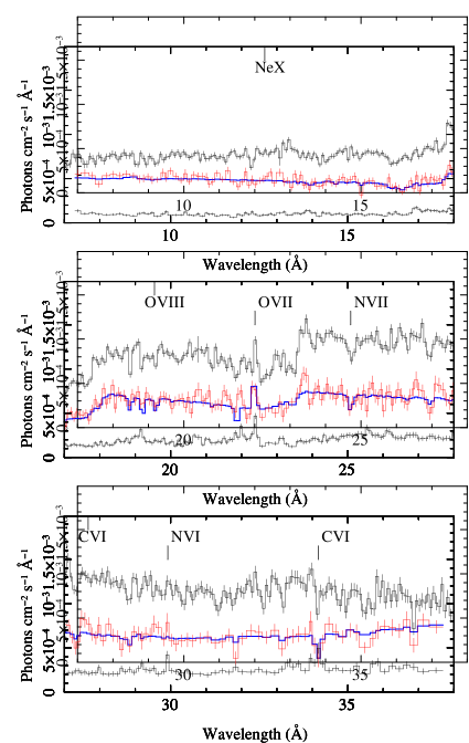
Figure 5: RGS data from the new observation (red) and the highest and lowest archival flux states (black) unfolded to a constant model. Emission lines are clearly visible in the low state, while absorption features are present in the high state. The blue line shows a fit with absorption and emission components applied to a phenomenological continuum. Wavelengths are given in the observed frame and the range of each panel overlaps the next by 1 Å.

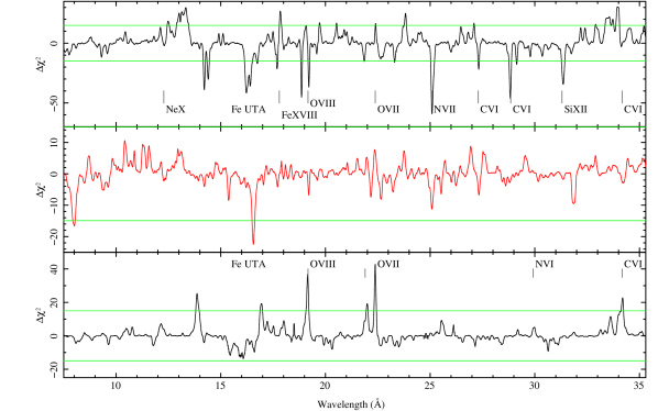
Figure 6: Results of line scans to the new data (middle) as well as the highest (top) and lowest (bottom) flux archival observations. The green lines show the 95 % confidence interval for a blind search.

Table 3: Narrow features in archival RGS spectra. Line wavelengths and transition levels are values from the APEC database. Redshifts are given in the observer’s frame (Mrk 766 is at $z=0.0129$).

Low state – emission

Species		Rest wavelength/Å	Redshift
C vi	2p1 – 1s1	33.736	$0.0130_{-0.0021}^{+0.0008}$
N vi	1s12s1 – 1s2	29.534	$0.0121_{-0.0004}^{+0.0009}$
O vii	1s12s1 – 1s2	22.098	$0.0128_{-0.0006}^{+0.0006}$
O viii	2p1 – 1s1	18.969	$0.0099_{-0.0010}^{+0.0012}$

High state – absorption

Species		Rest wavelength/Å	Redshift
Ne x	1s1 – 2p1	12.134	$0.0126_{-0.0014}^{+0.0017}$
N vii	1s1 – 2p1	24.781	$0.0132_{-0.0031}^{+0.0009}$
C vi	1s1 – 4p1	26.990	$0.0124_{-0.0006}^{+0.0004}$
C vi	1s1 – 2p1	33.736	$0.0117_{-0.0004}^{+0.0005}$

Warm absorption and emission are known to have an important effect on the spectrum of Mrk 766 in the soft band (e.g. Sako et al., 2003; Laha et al., 2014). To determine the nature of the gas which is responsible for these features, we begin by identifying features visually and with systematic line scans similar to those performed by for example Tombesi et al. (2010) and Pinto et al. (2016) with a phenomenological continuum (Fig. 6).

We use a broadband continuum model based on that of Branduardi-Raymont et al. (2001): a powerlaw with two broad lines. We then ensure that the local continuum is well-described with a cubic spline modification over the region $\pm 1$ Å from the wavelength of interest. We measure line significance from the change in $\chi^{2}$ when including an additional unresolved Gaussian at fixed wavelength, allowed to have positive or negative normalisation (one additional degree of freedom; the use of positive or negative normalisation in the same fit is needed to avoid the problems described in Protassov et al. 2002). We then scan the wavelength across the RGS range to find $\Delta\chi^{2}$ at each wavelength. We indicate approximate significance by estimating a critical $\Delta\chi^{2}_{\rm crit}$ for 95 % significance from the expected distribution of $N$ independent trials each having a $\chi_{1}^{2}$ distribution. We estimate the number, $N$ of independent trials performed by the wavelength range tested divided by the instrumental resolution, $(\lambda_{\rm max}-\lambda_{\rm min})/{\rm d}\lambda=450$. The global 95 % confidence interval (the solution $\Delta\chi^{2}_{\rm crit}$ to $P(\chi_{1}^{2}<\Delta\chi^{2}_{\rm crit})^{N}=0.95$) then corresponds to $\Delta\chi^{2}_{\rm crit}=14.9$ (shown as the green line in Fig. 6). We note also that changing the estimate of the effective number of independent trials has only a small effect on the critical $\Delta\chi^{2}_{\rm crit}$: increasing or decreasing the number of trials by a factor of 2 changes the critical $\Delta\chi^{2}_{\rm crit}$ to 16.2 or 13.6 respectively.

Since the new observations show few features at high significance (the XMM-Newton RGS observation is relatively shallow – 37,000 counts in total across both detectors and orders), we are also guided by the sensitive archival XMM-Newton RGS spectra from the highest and lowest previously observed states (Fig. 5; pn spectra shown in Fig. 2). While the absorbing material may not be identical in the XMM-Newton and NuSTAR exposures, the features found in the archival observations provide a guide from which to start modelling the latest data. Results of these line scans are shown in Fig. 6. Where a feature has a single most likely associated transition, we fit with a Gaussian to find the redshift of the feature. Results are shown in table 3. The lines are consistent with being unresolved.

The previous low-flux observation shows several emission lines (Table 3). The ionisation states of the observed lines suggest an ionisation parameter of $\log(\xi/{\rm erg\,cm\,s^{-1}})\sim 1.5$. Warm emission in AGN is usually predominantly photoionised (e.g. Guainazzi & Bianchi, 2007) and the high strength of the O vii forbidden line relative to the corresponding recombination line in this case supports this. Most of the lines are consistent with being in the rest frame of Mrk 766, but the most highly ionised O viii line is bluer, with a redshift corresponding to a projected outflow of $900_{-350}^{+300}$ km s^-1. We also note that the N vi line is larger than would be predicted based on Solar abundances. This is not unexpected as overly strong N vi lines have also been found in NGC 3516 (Turner et al., 2003).

In contrast, the high-flux spectrum principally shows absorption features (Table 3), with O vii the only previously identified emission line still seen in emission (the other emission lines are likely not visible due to their small equivalent width). Narrow features are present at wavelengths expected of C vi, N vii, and Ne x.

Since detailed modelling of the warm absorber is not the primary focus of this work, we do not attempt to fit the archival observations but fit the new observations with photoionisation models including the detected features. We use the photoionisation model XSTAR (Kallman & Bautista, 2001) and, for computational efficiency, fit using tables, which we compute for an appropriate region of parameter space.

Fitting the new observation with several warm-absorber components, we find that two ionisation states are sufficient ($\chi^{2}/{\rm d.o.f.}=1040/982=1.06$). With only one rather than two absorbing components, the fit is significantly worse ($\Delta\chi^{2}=36$ for 2 fewer degrees of freedom), as the absorption around the iron unresolved transition array (UTA) region ($\sim 17$ Å) is not sufficiently broad. Three absorbers provide insignificant improvement ($\Delta\chi^{2}=1.1$ for 2 additional degrees of freedom). It is likely that this two-component absorber represents a more complicated region of gas, but this parametrisation is sufficient to describe the absorber well enough to allow broadband continuum fitting.

When modelling the full dataset, we freeze the redshifts to appropriate values due to the large amount of low resolution data, which can drive the fitted redshift away from the values derived from the narrow RGS features. We fix the redshift of the warm absorbers to a value consistent with all the features observed in the high-flux spectrum, $z=0.0118$. Since the O viii line is not detected in the new observation, we model the line emission with a single component of photoionised gas at a redshift consistent with the O vii line.

3.3 Broadband fits

With a description of both the high-energy excesses and the warm absorber separately, we now perform a broadband fit to find a consistent model of the high and low energy features of the spectra. We include all data from NuSTAR, Swift, XMM-Newton-pn and XMM-Newton-RGS.

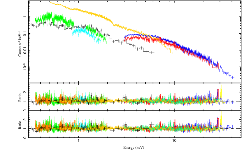
Figure 7: Data and residuals of best fitting broadband models. Top: data; middle: residuals for reflection model; bottom: residuals for partial covering model.

3.3.1 Reflection models

We first consider the reflection interpretation of the iron line and Compton hump. Combining the components found in each energy band results in a model of the form TBnew* (warmabs(1) * warmabs(2) * relxill + photemis).

Fits to each observation separately are given in Table 4. The parameters are largely consistent with those found in the individual band models.

The XMM-Newton/NuSTAR observation shows evidence of more emission coming from very close to the black hole than the Swift/NuSTAR observation. This is reflected in the emissivity index and reflection fraction being higher, which can both be induced by light-bending of radiation from a corona close to the black hole (Miniutti & Fabian, 2004).

The Swift/NuSTAR observation does not constrain the black hole spin, whereas the XMM-Newton/NuSTAR observation prefers $a>0.87$. The much stronger constraint in the XMM-Newton/NuSTAR observation is largely due to the much greater soft-band (<10 keV) signal from the XMM-Newton coverage. The remaining parameters of this observation also suggest that more emission is from the innermost region, which is most sensitive to the spin. The spin constraint from the XMM-Newton/NuSTAR observation is significantly higher than the fit to the high energy data only ($a<0.43$). This is likely to be because the spin measurement is significantly influenced by the shape of the soft excess and not just the profile of the iron line; the inconsistency could be due to other factors influencing the soft excess (as was found in e.g. Parker et al., 2018), such as the hybrid model discussed later.

The iron abundance of the XMM-Newton/NuSTAR observation is also higher. Since the material in the disc is not expected to change in the 6 months between observations, this is likely to be due to degeneracy with other parameters. If the difference is real, it could be caused by a higher iron abundance in the inner region of the disc, which the higher emissivity index suggests provides more of the reflected component in this observation. However, the data presented here are insufficient to prove this.

The cut-off of the powerlaw is too high to be measured with the current dataset and our lower limits are well outside the observed bandpass. The stronger limit for the Swift/NuSTAR observation is due to its greater high-energy signal from the longer NuSTAR exposure.

In order to improve constraints on the parameters of the model which do not change over the 6 month interval between the two observations and increase physical self-consistency, we also perform a joint fit with these parameters – black hole spin, $a$, accretion disc inclination, $i$, and iron abundance, $A_{\rm Fe}$ – tied between the two observations. Since the Swift spectrum does not significantly constrain the parameters of the absorption and emission, we also tie these parameters between the two observations. This fit is shown in Table 4 and Fig 7. The model spectrum is shown in Fig. 8. The parameters of this fit are largely consistent with the fits to the individual observations. Differences are likely due to parameter degeneracies which are not evident in single-parameter confidence intervals.

Table 4: Parameters of fits to all data from each observation with reflection model (TBnew * (warmabs(1) * warmabs(2) * relxill + photemis)). Unconstrained parameters are allowed to vary within the ranges: $-0.998<a<0.998$; $1<\log(\xi/{\rm erg\,cm\,s^{-1}})<2.5$; and $N_{\rm H}$/cm${}^{-2}<5\times 10^{22}$, indicated in the table by square brackets.

Component	Model	Parameter	Separate		Joint
			Swift/NuSTAR	XMM/NuSTAR	Swift/NuSTAR	XMM/NuSTAR
Relativistic reflection	(relxill)	Norm	$1.3\pm 0.1\times 10^{-4}$	$9.9_{-0.3}^{+0.1}\times 10^{-5}$	$1.24_{-0.04}^{+0.06}\times 10^{-4}$	$9.85_{-0.05}^{+0.04}\times 10^{-5}$
		Emissivity Index	$2.3_{-0.5}^{+0.7}$	$3.3_{-0.2}^{+0.4}$	$2.4\pm 0.2$	$4.5_{-0.4}^{+1.1}$
		$a$	Unconstrained	$>0.87$	$>0.92$
		$\theta/^{\circ}$	$47_{-4}^{+8}$	$36_{-2}^{+1}$	$46_{-4}^{+1}$
		$\Gamma$	$2.28_{-0.06}^{+0.08}$	$2.22_{-0.01}^{+0.02}$	$2.17_{-0.02}^{+0.01}$	$2.23\pm 0.02$
		$\log(\xi/{\rm erg\,cm\,s^{-1}})$	$1.7_{-0.4}^{+0.3}$	$1.4\pm 0.2$	$1.9_{-0.1}^{+0.1}$	$1.33_{-0.15}^{+0.03}$
		$A_{\rm Fe}$	$1.0_{-0.2}^{+0.8}$	$2.7_{-0.6}^{+0.7}$	$2.9_{-0.4}^{+0.7}$
		$E_{\rm cut}$/keV	$>290$	$>530$	$>510$	$>740$
		$R$	$1.4_{-0.3}^{+0.5}$	$1.8_{-0.3}^{+0.4}$	$0.9_{-0.1}^{+0.2}$	$2.1\pm 0.4$
Ionised absorption	(warmabs)	$N_{\rm H}$/cm-2	$<4.7\times 10^{21}$	$2.0_{-0.4}^{+0.6}\times 10^{21}$	$1.8_{-0.4}^{+0.5}\times 10^{21}$
		$\log(\xi/{\rm erg\,cm\,s^{-1}})$	$[1-2.5]$	$1.96_{-0.04}^{+0.07}$	$1.97_{-0.06}^{+0.07}$
		$N_{\rm H}$/cm-2	$<4.9\times 10^{21}$	$2.0\pm 0.3\times 10^{21}$	$2.1_{-0.2}^{+0.3}\times 10^{21}$
		$\log(\xi/{\rm erg\,cm\,s^{-1}})$	$[1-2.5]$	$1.31_{-0.04}^{+0.05}$	$1.29\pm 0.04$
Ionised emission	(photemis)	Norm	$<0.047$	$2.6_{-2.1}^{+0.4}\times 10^{-4}$	$2.5_{-1.9}^{+0.5}\times 10^{-4}$
		$N_{\rm H}$/cm-2	$[<5\times 10^{22}]$	$<5\times 10^{21}$	$[<5\times 10^{22}]$
		$\log(\xi/{\rm erg\,cm\,s^{-1}})$	$[1-2.5]$	$1.5\pm 0.1$	$1.5\pm 0.1$
Cross-calibration constant		FPMA/XRT	$1.15_{-0.08}^{+0.10}$	-	$1.14\pm 0.03$
		FPMB/XRT	$1.14_{-0.08}^{+0.09}$	-	$1.13\pm 0.03$
		RGS1 order 1/PN	-	$1.00\pm 0.02$	$1.00\pm 0.02$
		RGS2 order 1/PN	-	$1.01\pm 0.02$	$1.01\pm 0.02$
		RGS1 order 2/PN	-	$0.99\pm 0.04$	$0.99\pm 0.04$
		RGS2 order 2/PN	-	$0.97\pm 0.04$	$0.97\pm 0.04$
		FPMA/PN	-	$1.15_{-0.02}^{+0.03}$	$1.15_{-0.03}^{+0.02}$
		FPMB/PN	-	$1.13_{-0.02}^{+0.03}$	$1.13_{-0.03}^{+0.02}$
$\chi^{2}$ (bins)					990 (884)	2262 (2202)
$\chi^{2}/$d.o.f.			$974.7/866=1.13$	$2238/2180=1.03$	$3252/3056=1.06$

3.3.2 Partial covering models

We also make a broadband fit with a partial covering model of the form TBnew * zpcfabs(1) * zpcfabs(2) * (warmabs(1) * warmabs(2) * cutoffpl + photemis). Parameters for this model are given in Table 5; residuals are shown in Fig. 7 and model spectra in Fig. 8.

Table 5: Parameters of fits to all data from each observation with partial covering model (TBnew * zpcfabs(1) * zpcfabs(2) * (warmabs(1) * warmabs(2) * cutoffpl + photemis)). Unconstrained parameters are allowed to vary within the ranges: $1<\log(\xi/{\rm erg\,cm\,s^{-1}})<2.5$; and $N_{\rm H}$/cm${}^{-2}<5\times 10^{22}$, indicated in the table by square brackets.

Component	Model	Parameter	Separate		Joint
			Swift/NuSTAR	XMM/NuSTAR	Swift/NuSTAR	XMM/NuSTAR
Partial covering absorber	(zpcfabs)	$N_{\rm H}$/cm-2	$7.2_{-1.1}^{+1.2}\times 10^{24}$	$5.5_{-0.6}^{+1.3}\times 10^{24}$	$1.2_{-0.1}^{+0.13}\times 10^{25}$	$5.2_{-0.6}^{+1.2}\times 10^{24}$
		$f_{\rm Cov}$	$0.64_{-0.07}^{+0.03}$	$0.51_{-0.03}^{+0.05}$	$0.69_{-0.06}^{+0.05}$	$0.51_{-0.03}^{+0.05}$
	(zpcfabs)	$N_{\rm H}$/cm-2	$6.2_{-1.1}^{+0.7}\times 10^{23}$	$2.0_{-0.2}^{+0}\times 10^{23}$	$1.0\pm 0.15\times 10^{24}$	$1.9_{-0.2}^{+0}\times 10^{23}$
		$f_{\rm Cov}$	$0.41_{-0.03}^{+0.04}$	$0.361_{-0.003}^{+0}$	$0.43\pm 0.06$	$0.356_{-0.003}^{+0.018}$
Primary cut-off powerlaw	(cutoffpl)	Norm	$0.052_{-0.006}^{+0.014}$	$0.028\pm 0.001$	$0.06\pm 0.01$	$0.0276_{-0.0023}^{+0.0001}$
		$\Gamma$	$2.14_{-0.08}^{+0.10}$	$2.33_{-0.004}^{+0.02}$	$2.12\pm 0.06$	$2.33\pm 0.02$
		$E_{\rm Cut}$/keV	$26_{-6}^{+0}$	$>190$	$22_{-5}^{+7}$	$>180$
Ionised absorption	(warmabs)	$N_{\rm H}$/cm-2	$<8.8\times 10^{21}$	$3.3_{-0.2}^{+0}\times 10^{21}$	$3.16_{-0.17}^{+0}\times 10^{21}$
		$\log(\xi/{\rm erg\,cm\,s^{-1}})$	$>1.2$	$2.06_{-0.05}^{+0.03}$	$2.05_{-0.05}^{+0.03}$
		$N_{\rm H}$/cm-2	$<4.6\times 10^{21}$	$2.30_{-0.06}^{+0}\times 10^{21}$	$2.29_{-0.06}^{+0}\times 10^{21}$
		$\log(\xi/{\rm erg\,cm\,s^{-1}})$	$[1-2.5]$	$1.39\pm 0.03$	$1.40_{-0.05}^{+0.04}$
Ionised emission	(photemis)	Norm	$<1.1\times 10^{-2}$	$3.4_{-2.4}^{+0.6}\times 10^{-4}$	$1.6_{-1.5}^{+0.3}\times 10^{-3}$
		$N_{\rm H}$/cm-2	$[<5\times 10^{22}]$	$<1.7\times 10^{21}$	$<1.3\times 10^{21}$
		$\log(\xi/{\rm erg\,cm\,s^{-1}})$	$>1.3$	$1.55_{-0.08}^{+0.07}$	$1.53\pm 0.08$
Cross-calibration constant		FPMA/XRT	$1.14_{-0.08}^{+0.09}$	-	$1.14_{-0.05}^{+0.08}$
		FPMB/XRT	$1.13_{-0.08}^{+0.09}$	-	$1.13_{-0.05}^{+0.08}$
		RGS1 order 1/PN	-	$1.00\pm 0.02$	$0.96\pm 0.02$
		RGS2 order 1/PN	-	$1.00\pm 0.02$	$0.95\pm 0.02$
		RGS1 order 2/PN	-	$0.97\pm 0.04$	$0.92\pm 0.04$
		RGS2 order 2/PN	-	$0.96\pm 0.04$	$0.93\pm 0.04$
		FPMA/PN	-	$1.12_{-0.03}^{+0.02}$	$1.12_{-0.03}^{+0.02}$
		FMPB/PN	-	$1.10_{-0.03}^{+0.02}$	$1.10_{-0.03}^{+0.02}$
$\chi^{2}$ (bins)					980 (884)	2339 (2202)
$\chi^{2}/$d.o.f.			$974.2/868=1.12$	$2297/2182=1.05$	$3319/3057=1.09$

While this produces an acceptable fit to the spectrum, some parameters are not physically likely. In particular, the high-energy cut-off of $22_{-5}^{+7}$ keV in the Swift/NuSTAR observation is much lower than is typically found in AGN (e.g. Fabian et al., 2015; Lubiński et al., 2016) and below the lowest found so far with NuSTAR data ($42\pm 3$ keV in Ark 564, Kara et al. 2017). The time-averaged Swift-BAT spectrum does not show such a low cut-off energy (e.g. Vasudevan et al., 2010; Ricci et al., 2017), although the coronal temperature may change with time. This is corroborated by the low cut-off not being present in the XMM-Newton/NuSTAR observation, which is detected only up to 35 keV, below the far side of the Compton hump. Forcing the cut-off to be at least 100 keV results in a significantly worse fit ($\Delta\chi^{2}=18.5$). The low cut-off value may be due to curvature from the high-energy side of the Compton hump being accounted for by an artificially low cut-off energy. A high column density component ($N_{\rm H}=1.2_{-0.1}^{+0.13}\times 10^{25}$ cm^-2) is then required to produce the low-energy side of the Compton hump.

The large absorbing column density also implies a high unabsorbed luminosity: $L_{\rm 0.5-10\,keV}=7.5\times 10^{43}$ erg s^-1 for the Swift/NuSTAR observation. This is not compatible with the bolometric luminosity of $10^{44}$ erg s^-1 found by SED fitting (Vasudevan et al., 2010) which must also include significant intrinsic disc emission.

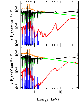
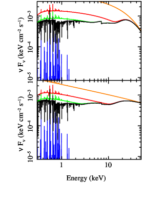
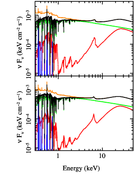
Figure 8: Plot of models found for joint fit. Left panels: reflection models; Centre panels: partial covering models; Right panels: hybrid models. Top panels: Swift/NuSTAR observation; Bottom panels: XMM-Newton/NuSTAR observation. Black: total model; Orange: unabsorbed model; Blue: photoionised emission; Reflection/hybrid models: Green: powerlaw continuum; Red: reflected component. Partial covering models: Green: two partial covering components without ionised absorption; Red: one partial covering component.

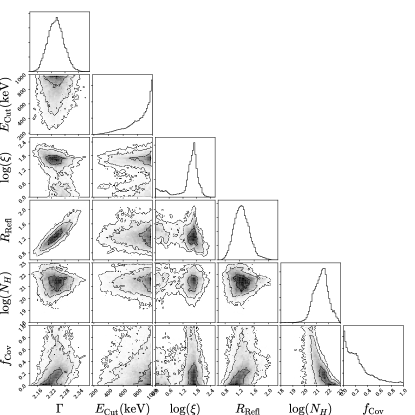
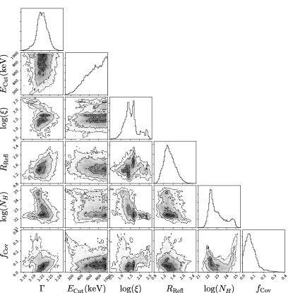
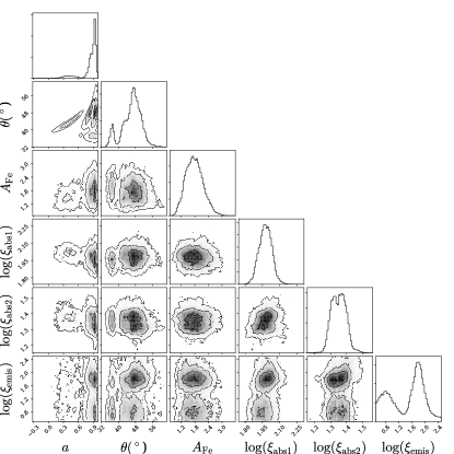
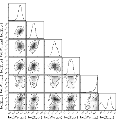
Figure 9: Corner plots of MCMC parameter estimation for a hybrid model with reflection and partial covering. Parameters shown in each panel are: top left: Swift/NuSTAR observation; top right: XMM-Newton/NuSTAR observation; bottom left: parameters tied between observations; bottom right: warm absorption/emission. Column densities have units of cm^-2; $\xi$ has units of erg cm s^-1. Contours indicate 1,2, and 3$\sigma$ intervals.

3.3.3 Hybrid models

Further to the extreme scenarios in which only reflection or only absorption are responsible for the spectrum of Mrk 766, we consider a model which includes both of these effects. We use a model of the form TBnew * zpcfabs(1) * (warmabs(1) * warmabs(2) * relxill + photemis). Due to the potential for strong degeneracy between the two possible causes (relativistic emission and partial covering absorption) for the spectral shape, we use Monte-Carlo methods to sample the parameter space. We use the XSPEC_EMCEE code. We use 600 walkers and take probability densities from 10000 iterations after the chain has converged. Results are shown in table 6 and Fig. 9.

Note that we have shown the $\chi^{2}$ value from direct minimisation for comparison with other models; the parameters from the two methods are consistent.

The reflection parameters found are largely consistent with those found for the pure reflection case, with less strict confidence limits. The iron abundance is somewhat lower, being slightly closer to Solar, and the reflection fraction of the XMM-Newton/NuSTAR observation is closer to unity. The constraint on the spin is significantly weaker. The parameters of the absorption are much less extreme than the pure partial covering model. We now find solutions with column densities $N_{\rm H}\simeq 10^{22-23}$ cm^-2, which is more reasonable given the lack of a strong narrow iron line, which would be expected with the higher columns required for the pure partial covering model. In general, the hybrid model requires less extreme parameters than either reflection or partial covering alone.

Table 6: Parameters of fits to all data from each observation with model including partial covering and reflection TBnew * zpcfabs(1) * (warmabs(1) * warmabs(2) * relxill + photemis). Parameters given are the median of the posterior distribution; errors correspond to the central 90% of the MCMC posterior distribution. The $\chi^{2}$ value refers to the value found by $\chi^{2}$-minimisation. Unconstrained parameters are allowed to vary within the ranges: $1<\log(\xi/{\rm erg\,cm\,s^{-1}})<2.5$; and $N_{\rm H}$/cm${}^{-2}<5\times 10^{22}$, indicated in the table by square brackets.

Component	Model	Parameter	Joint
			Swift/NuSTAR	XMM/NuSTAR
Relativistic reflection	(relxill)	Norm	$1.30\pm 0.04\times 10^{-4}$	$1.02_{-0.03}^{+0.06}\times 10^{-4}$
		Emissivity Index	$2.2_{-0.6}^{+0.4}$	$5.5_{-1.0}^{+1.7}$
		$a$	$>0.4$
		$\theta$	$47_{-10}^{+6}$
		$\Gamma$	$2.24\pm 0.06$	$2.22\pm 0.03$
		$\log(\xi/{\rm erg\,cm\,s^{-1}})$	$1.6_{-1.4}^{+0.4}$	$1.5_{-0.5}^{+0.8}$
		$A_{\rm Fe}$	$1.8_{-0.6}^{+0.7}$
		$E_{\rm cut}$	$>490$	$>350$
		$R$	$1.25_{-0.3}^{+0.4}$	$1.4_{-0.3}^{+0.4}$
Partial covering absorption	(zpcfabs)	$N_{\rm H}$/cm-2	$<2.3\times 10^{22}$	$5_{-1}^{+500}\times 10^{22}$
		$f_{\rm Cov}$	$<0.75$	$0.07_{-0.06}^{+0.12}$
Ionised absorption	(warmabs)	$N_{\rm H}$/cm-2	$2.1_{-0.6}^{+0.8}\times 10^{21}$
		$\log(\xi/{\rm erg\,cm\,s^{-1}})$	$1.98\pm 0.09$
		$N_{\rm H}$/cm-2	$1.8_{-0.3}^{+0.4}\times 10^{21}$
		$\log(\xi/{\rm erg\,cm\,s^{-1}})$	$1.35\pm 0.07$
Ionised emission	(photemis)	Norm	$1.2_{-0.8}^{+0.3}\times 10^{-5}$
		$N_{\rm H}$/cm-2	$[<5\times 10^{22}]$
		$\log(\xi/{\rm erg\,cm\,s^{-1}})$	$1.6_{-1.0}^{+0.5}$
$\chi^{2}$ (bins)			979 (884)	2267 (2202)
$\chi^{2}/$d.o.f.			$3246/3052=1.06$

3.4 Variability

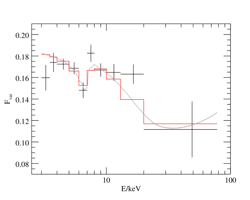
Figure 10: The fractional excess variance for Mrk 766 computed using the entire light curve of the longer observation in time bins of 400 s. The variability drops in the iron K and Compton hump regions. This can be explained by a variable continuum and a constant reflection component (grey; binned to data resolution in red).

To characterize the rapid variability in this source, we compute the fractional excess variance in the NuSTAR spectrum, binned to 400 s, using the prescription in Edelson et al. (2002) with errors from the formula in Vaughan et al. (2003b). We use the fractional variability rather than Fourier methods owing to the former’s insensitivity to the orbital gaps in NuSTAR observations (e.g. Nandra et al., 1997a). The shorter XMM-Newton/NuSTAR observation only has enough signal to produce two energy bins, which are broadly consistent with the results from the longer observation, so we only present detailed results from the longer observation here (Fig. 10).

The variability appears reduced in the $6-7$ keV band, the rest energy of iron K, and above 10 keV, where the Compton reflection hump provides significant flux in the mean spectrum. Overall, the decrease in variability on short timescales appears to follow the profile of the relativistic reflection features, which suggests that the reflection component does not vary as much as the continuum emission in Mrk 766. This is reminiscent of previous spectral-timing results of MCG–6-30-15 that also showed that the continuum varies more than the ionised reflection (Vaughan et al., 2003a; Fabian & Vaughan, 2003; Marinucci et al., 2014). The increase in variability in the $7-8$ keV bin may be due to variable blueshifted absorption (Risaliti et al., 2011; Parker et al., 2017).

We can test whether this $F_{\rm Var}$ spectrum is compatible with a variable continuum and less variable reflection by considering the extreme case in which the reflection is constant, so only the power law varies. Denoting the mean reflected flux as $f_{\rm R}(E)$, the mean continuum as $f_{\rm C}(E)$ and the variance as $\alpha^{2}f_{\rm C}^{2}$ (i.e. the variability is a constant multiple of the continuum flux), the fractional variability is simply

$$F_{\rm Var}(E)=\alpha\frac{f_{\rm C}(E)}{f_{\rm C}(E)+f_{\rm R}(E)}.$$

Thus, higher $\alpha$ leads to higher $F_{\rm Var}$ while the shape of $F_{\rm Var}$ is set by the shape of the reflected spectrum, which we take from the fit to the mean spectrum. We may then substitute for the mean fluxes found in our fits to the mean spectrum and fit the observed $F_{\rm Var}(E)$ values (by $\chi^{2}$-minimisation) to find $\alpha$. This gives an acceptable fit, $\chi^{2}/{\rm d.o.f.}=16/9$, $p=0.07$.

In the partial covering scenario, the $>20$ keV bin shows intrinsic continuum variability (since there is little absorption at these energies) while the greater variability at lower energies is due to variable absorption strength or continuum pivoting. We do not attempt to fit this as covariance between different variability mechanisms rapidly introduces more free parameters than can be constrained by the available data.

4 Discussion

4.1 The reflection model

We note that the presence of distant cold reflection is not required in either observation. This may be due to the relativistic reflection already including a significant component of weakly blurred reflection from a low emissivity index ($2.4\pm 0.2$ in the Swift/NuSTAR observation). The lack of a distinct distant component could also be due to absorption reducing the X-ray flux to distant regions of the disc and to the torus, weakening the cold reflection. Since the warm absorber in our line of sight ($\sim 50^{\circ}$ from the disc plane) has only a small effect on the transmitted flux, this mechanism would require more absorption in the line of sight of the outer disc and torus. Such absorption would also reduce the correlation between X-ray emission and reprocessing from the disc, consistent with the non-detection of correlated UV/X-ray lags in Buisson et al. (2017). The warm absorption also complicates the spectrum, increasing the uncertainty on the amount of cold reflection and so reducing the significance of any detection.

The lower limit on the cut-off of the primary continuum is higher than is typically found in AGN (Fabian et al., 2015; Lubiński et al., 2016). However, the limit presented here is far outside the NuSTAR bandpass so is strongly affected by the shape of the reflected part of the spectrum rather than being a direct measurement of the cut-off (García et al., 2015). Due to the complex absorption in Mrk 766, these features are harder to accurately isolate and so the cut-off may be significantly lower than the statistical limit presented here. The difference in curvature below the cut-off energy between a cut-off powerlaw and a true Comptonisation spectrum may also allow for a lower coronal temperature (Fürst et al., 2016).

4.2 Comparison with a similar source, MCG–6-30-15

MCG–6-30-15 is a very well studied AGN with similar spectral appearance to Mrk 766 (and similar Principal Components of variability, Parker et al. 2015); we therefore compare our interpretations with those found for MCG–6-30-15. Marinucci et al. (2014) study spectral variability in the available NuSTAR data, considering both reflection and partial covering models. The higher count rate of MCG–6-30-15 allows the observation to be cut into 11 sections. In the reflection interpretation, $a=0.91_{-0.07}^{+0.06}$, $i=33\pm 3^{\circ}$, similar to values found here and in previous works for Mrk 766 (e.g. Branduardi-Raymont et al., 2001).

A detailed analysis of grating spectra of MCG–6-30-15 from RGS by Sako et al. (2003); Turner et al. (2004) and from Chandra by Holczer et al. (2010) shows two intrinsic absorption systems with distinct velocities, outflowing at $100\pm 50$ and $1900\pm 150$ km s^-1. The absorption considered in our model is comparable to the lower speed component (in our case with fixed outflow velocity of 350 km s^-1 based on archival line positions) while the fast component in MCG–6-30-15 is too highly ionised ($\log(\xi/{\rm erg\,cm\,s^{-1}})=3.82\pm 0.03$) to have a noticeable effect in the short RGS exposure studied here.

The slow component in MCG–6-30-15 has an ionisation parameter ranging from $\log(\xi/{\rm erg\,cm\,s^{-1}})=-1.5$ to $\log(\xi/{\rm erg\,cm\,s^{-1}})=3.5$, while the two ionisations we consider have $\log(\xi/{\rm erg\,cm\,s^{-1}})\sim 1.3$ and $1.9$. Holczer et al. (2010) also find little gas with $0.5<\log(\xi/{\rm erg\,cm\,s^{-1}})<1.5$ so our component with $\log(\xi/{\rm erg\,cm\,s^{-1}})\sim 1.3$ may reflect a mixture of more and less ionised gas. This is plausible since the CCD spectra of MCG–6-30-15 may be described with a two-state warm absorber with ionisation parameters of $\log(\xi/{\rm erg\,cm\,s^{-1}})\simeq 2$ and $\log(\xi/{\rm erg\,cm\,s^{-1}})=1.15-1.65$ (Marinucci et al., 2014).

Emmanoulopoulos et al. (2011) find soft lags in the X-ray light curves of both Mrk 766 and MCG–6-30-15 (as do Kara et al. 2014), which are interpreted as arising from the delay of reflected emission. Parker et al. (2014a) study the variability of MCG–6-30-15 with Principal Component Analysis (PCA), finding that the variability is consistent with that expected from an intrinsically variable X-ray source with less variable relativistic reflection. This is corroborated by Miniutti et al. (2007), who calculate the RMS (fractional variability) spectrum of a Suzaku observation of MCG–6-30-15, which has a similar shape to the short timescale $F_{\rm Var}$ spectrum found here. This could arise from a vertically extended or two component corona, in which, due to strong light bending, the lower portion principally illuminates the disc while the upper region is responsible for the majority of the direct emission. This would also decorrelate the observed X-ray emission from any UV variability which is driven by disc heating, agreeing with the lack of correlation seen in these two sources (Buisson et al., 2017). In the observations presented here, Mrk 766 remains in a high state, so it is hard to find evidence of coronal extension from variability.

4.3 Distinguishing absorption from reflection

While variable partial covering absorption and reflection both provide acceptable fits to the data, the reflection model is favoured for the following reasons:

• the partial covering model gives a high unabsorbed luminosity ($L_{\rm 0.5-10\,keV}=7\times 10^{43}$ erg s^-1), which is incompatible with previous directly integrated measurements of the bolometric luminosity (Vasudevan et al., 2010).

• the high-energy continuum cut-off of $22_{-5}^{+7}$ keV is very low in the partial covering model of the Swift/NuSTAR observation (although some recent NuSTAR observations have found low cut-offs in other sources, e.g. $53_{-8}^{+11}$ keV, Tortosa et al. 2017; $42\pm 3$ keV, Kara et al. 2017);

• the PCA analysis in Parker et al. (2015) shows that Mrk 766 varies in the same way as MCG–6-30-15, showing the behaviour of a source whose variability is explained well by relativistic reflection from a vertically extended corona;

• the fractional variability spectrum shows a clear dip in the shape of the iron line, as would be produced by a variable continuum and less variable reflection.

5 Conclusions

We have presented two new observations of Mrk 766 taken by NuSTAR, providing a detailed view of its hard X-ray spectrum. With simultaneous coverage in soft X-rays by XMM-Newton or Swift, we are able to exploit the high spectral resolution of XMM-Newton-RGS to take account of warm absorption and so produce better constraints on the broadband spectrum.

We can model the spectrum with reflection or partial covering to generate the iron K feature and Compton hump. In the reflection model, the system has a high spin black hole ($a>0.92$) viewed at intermediate inclination ($i=46_{-2}^{+1}\,{}^{\circ}$). The best-fitting partial covering model is questionable as it requires a very low cut-off energy and the intrinsic X-ray luminosity is high compared to the bolometric luminosity. A hybrid model including reflection and partial covering allows less extreme conditions for each component of the model.

References

- Baloković et al. (2015) Baloković M., et al., 2015, ApJ, 800, 62
- Bentz et al. (2009) Bentz M. C., et al., 2009, ApJ, 705, 199
- Bentz et al. (2010) Bentz M. C., et al., 2010, ApJ, 716, 993
- Branduardi-Raymont et al. (2001) Branduardi-Raymont G., Sako M., Kahn S. M., Brinkman A. C., Kaastra J. S., Page M. J., 2001, A&A, 365, L140
- Brenneman et al. (2014) Brenneman L. W., et al., 2014, ApJ, 788, 61
- Buisson et al. (2017) Buisson D. J. K., Lohfink A. M., Alston W. N., Fabian A. C., 2017, MNRAS, 464, 3194
- Dauser et al. (2010) Dauser T., Wilms J., Reynolds C. S., Brenneman L. W., 2010, MNRAS, 409, 1534
- De Marco et al. (2013) De Marco B., Ponti G., Cappi M., Dadina M., Uttley P., Cackett E. M., Fabian A. C., Miniutti G., 2013, MNRAS, 431, 2441
- Edelson et al. (2002) Edelson R., Turner T. J., Pounds K., Vaughan S., Markowitz A., Marshall H., Dobbie P., Warwick R., 2002, ApJ, 568, 610