Gravity’s Islands: Parametrizing Horndeski Stability

Abstract

Cosmic acceleration may be due to modified gravity, with effective field theory or property functions describing the theory. Connection to cosmological observations through practical parametrization of these functions is difficult and also faces the issue that not all assumed time dependence or parts of parameter space give a stable theory. We investigate the relation between parametrization and stability in Horndeski gravity, showing that the results are highly dependent on the function parametrization. This can cause misinterpretations of cosmological observations, hiding and even ruling out key theoretical signatures. We discuss approaches and constraints that can be placed on the property functions and scalar sound speed to preserve some observational properties, but find that parametrizations closest to the observations, e.g. in terms of the gravitational strengths, offer more robust physical interpretations. In addition we present an example of how future observations of the B-mode polarization of the cosmic microwave background from primordial gravitational waves can probe different aspects of gravity.

I Introduction

Acceleration of the cosmic expansion is a signal of new physics: a cosmological constant vacuum energy, a new scalar field, or new laws of gravity. As we extend the standard model into new theories, we must ensure that the foundation is sound and internally consistent. In particular, the theory should be free of pathologies such as ghosts and instabilities. For modified gravity, there is a wide class within effective field theory, Horndeski gravity the most general scalar-tensor theory with second order equations of motions, that has four free functions of time in addition to the cosmic background expansion. These can also be viewed as four property functions, describing properties of the scalar and tensor sectors and their mixing Bellini:2014fua .

Parametrization of these functions in a physically meaningful way – with a clear connection to observables and a sound theoretical foundation – has been a challenging task fraught with pitfalls 1512.06180 ; 1607.03113 . (Also see, e.g., 1705.01960 ; 1505.00174 ; koyama for some theory characteristics dealing with the field definitions rather than the property functions.) Here we examine this in terms of sensitivity and characteristics, concentrating on stability from the theoretical side, while also investigating the impact of very general observational considerations such as agreement with general relativity at early times and possessing characteristics consistent with the late time expansion history (e.g. a de Sitter limit). Recently, Kennedy:2018gtx has proposed the interesting idea of using stability, in terms of the sound speed of scalar perturbations, as the quantity to parametrize and deriving the property function behavior from this. In our analysis of the function space, and its relation to stability, we can assess the utility and generality of that approach, in addition to elucidating the characteristics of the property function space.

Furthermore, we explore the sensitivity to the parametrization used on the physical results and constraints. For example, Mueller:2016kpu demonstrated that the strength of modified gravity constraints could vary by almost two orders of magnitude depending on time dependence and priors assumed. This is a key question for the utility and robustness of comparing theory quantities such as property functions or sound speed to observables such as growth and clustering of matter structure and light deflection (gravitational lensing).

In Section II we scan through property function space and elucidate the relation between stability and functional parametrization, and also give an example of an observational effect by calculating the B-mode CMB polarization signature of the property functions. We discuss specific theories in Section III and compare to analytic stability results. Section IV examines the approach of using an explicitly stable parametrization of sound speed to map out the stable regions of property function space. In Section V we discuss observationally related issues such as the implications for the modified Poisson equation gravitational strengths $G_{\rm matter}$ and $G_{\rm light}$, and the impact of a general relativity past and de Sitter asymptotic future on acceptable parametrizations and stability. We conclude in Section VI.

II Property Function Space

II.1 Property Function Basics

The property function approach of Bellini:2014fua is a form of effective field theory for the gravitational action. Within Horndeski gravity, the most general scalar-tensor theory giving second order field equations, this involves four functions of time: $\alpha_{\_}K$, $\alpha_{\_}B$, $\alpha_{\_}M$, and $\alpha_{\_}T$, in addition to the background expansion given by the Hubble parameter $H(a)$. One of the attractions of this approach is that each function describes a physical property or characteristic of theory – respectively the structure of the kinetic term, the braiding of the scalar and tensor sectors, the running of the Planck mass, and the speed of gravitational wave propagation.

By specifying the form and parameters of the time dependent $\alpha$ functions one picks a particular theory of gravity. However, not every such theory may be sound: they may exhibit a gradient (Laplace) instability or may suffer from ghosts, rendering the theory unviable. Thus one must check the assumed parametrization of the property functions to assure the absence of such pathologies.

The no ghost condition is easily tested, as it involves a simple combination of the kineticity $\alpha_{\_}K$ and braiding $\alpha_{\_}B$ functions, requiring the condition

$$\alpha\equiv\alpha_{\_}K+(3/2)\alpha_{\_}B^{2}\geq 0$$ (1)

be satisfied. As long as we choose $\alpha_{\_}K\geq 0$ this will hold. This also automatically makes the denominator of the sound speed (see below) positive as well.

To guarantee the theory of gravity is free of gradient instability, the form (and parameters) of the time evolution of property functions must ensure the positivity of the speed of sound. As we see below, it is natural to set $\alpha_{\_}T=0$ and so the simple analytic expression for the speed of sound becomes

$$c_{\_}s^{2}=\frac{(1-\alpha_{\_}B/2)(2\alpha_{\_}M+\alpha_{\_}B)+(\alpha_{\_}B/2)(\ln H^{2})^{\prime}+\alpha^{\prime}_{\_}B}{\alpha_{\_}K+(3/2)\alpha_{\_}B^{2}}\ ,$$ (2)

where a prime denotes $d/d\ln a$. The stability condition is then $c_{\_}s^{2}>0$, and as mentioned above, this becomes a condition on nonnegativity of the numerator.

There are a number of publicly available Boltzmann codes, e.g. Zumalacarregui:2016pph ; Raveri:2014cka , going beyond general relativity by implementing property functions. These can be used for calculating the cosmic microwave background (CMB) temperature and polarization power spectra and the growth of matter density perturbations and the matter power spectrum. They also test for stability and ghosts (though we can use the above analytic equations for this). However, the public versions of these codes are limited in the functional forms usable for the property functions (while user defined function modules will eventually be implemented in the public versions, they are not yet there in a robust state). We therefore use them with the implemented power law form of the time evolution.

Testing stability is a critical first step in comparing theories to data, and extracting meaningful cosmological information. For this, we use the analytic expressions in Eq. (1) and (2), though we have tested our results against the Boltzmann code hi_class. Of particular interest is the role of the property function parametrization assumed on which theories are allowed. That is, for what time dependence forms, and what values of parameters within the forms, do we select which parts of property function parameter space. More seriously, does the parametrization bias the physical interpretation, such as implicitly disfavoring standard theories such as $f(R)$ gravity?

II.2 Checking Stability

Of the four property functions, the two with the greatest impact on cosmic survey observables are $\alpha_{\_}M$ and $\alpha_{\_}B$. The $\alpha_{\_}K$ function has minimal effect on subhorizon scales Bellini:2014fua and we set it to a small value that does not affect the results (recall it does not enter into the numerator of Eq. 2). The gravitational wave speed $c_{\_}T^{2}=1+\alpha_{\_}T$ has been tightly restricted to be close to one, i.e. $|\alpha_{\_}T|\lesssim 10^{-15}$, at present by gravitational wave and electromagnetic counterpart observations ligo . While this does not guarantee $\alpha_{\_}T(a)=0$ for all times (see, e.g., 1803.06368 ; 1802.09447 ; derham ), that is the simplest case and we adopt $\alpha_{\_}T=0$.

Thus we are interested in the $\alpha_{\_}M$–$\alpha_{\_}B$ space. For the power law time dependence we initially consider (see Secs. IV and V for other cases), $\alpha_{\_}i(a)=\alpha_{\_}{i,0}a^{s}$ where $a$ is the cosmic scale factor and a subscript 0 denotes the present value. The first important aspect to note is that restricting the parameter space, i.e. the amplitudes $\alpha_{\_}{i,0}$, too much can miss structure in the parameter space. Indeed, we will find “islands” appearing at larger $\alpha_{\_}{i,0}$ that might otherwise have not been found. Recall that the background expansion history, i.e. the Hubble parameter $H(a)$, is specified independently of the property functions. For concreteness and agreement with observations we take it to be given by the concordance flat $\Lambda$CDM cosmology, with present dimensionless matter density $\Omega_{m}=0.3$. For property function and some related studies away from $\Lambda$CDM, see for example Raveri:2014cka ; Peirone:2017lgi ; 1703.05297 .

Figure 1 shows how the shape of the stability region changes as we vary the scale factor at which the gradient stability is evaluated, here for $s=1$. At $a=1$ it extends into both left upper and right lower parts of the adopted parameter range with each part pinching in close to the origin in an hourglass shape. Smaller values of $a$ cut out most of the lower region, with intermediate values of the scale factor further diminishing this only slightly. The overall stability of the theory is determined by the intersection of the stable regions for all scale factors under consideration.

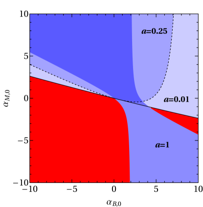
Figure 1: Evolution of stability regions in the $\alpha_{\_}{B,0}$ and $\alpha_{\_}{M,0}$ plane, for $\alpha_{\_}i=\alpha_{\_}{i,0}a^{1}$, obtained by varying the scale factor $a=0.01,0.25,1$ are represented with different levels of blue color from light to dark. The dashed line denotes the boundary of the stability region at $a=0.25$ and solid black line shows the boundary between the upper stability and lower instability regions at $a=0.01$. The red region is unstable for all these scale factors. The intersection of the stable regions for all scale factors gives the viable parameter space.

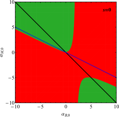
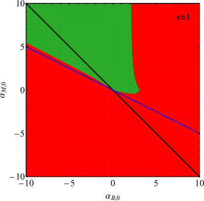
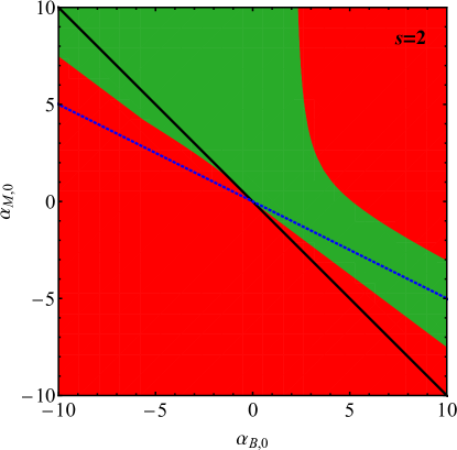
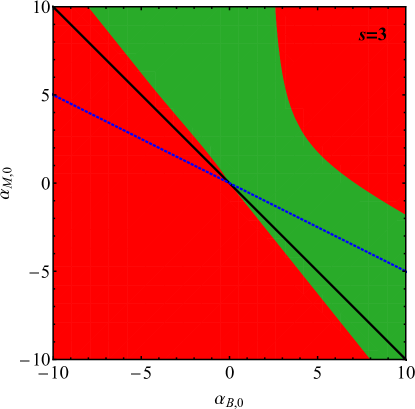
Figure 2: Regions of stability (green) and gradient instability (red) plotted in the $\alpha_{\_}{B,0}$ and $\alpha_{\_}{M,0}$ plane determined over the range of scale factors $a=[0.001,1]$ for $\alpha_{\_}i=\alpha_{\_}{i,0}a^{s}$ and $s=0,1,2,3$. Black solid line corresponds to $f(R)$ theories ($\alpha_{\_}B=-\alpha_{\_}M$), blue dotted line corresponds to No Slip Gravity ($\alpha_{\_}B=-2\,\alpha_{\_}M$).

Figure 2 gives a clear illustration of how the viability of a model depends on its parametrization. Even within the family of power law scale factor dependence $a^{s}$, the regions of stability exhibit different geometries. The time independent case ($s=0$) shows disjoint islands of stability, while $s=1$ is mostly restricted to positive $\alpha_{M,0}$ and negative $\alpha_{\_}{B,0}$. As $s$ increases further, a tail develops to negative $\alpha_{M,0}$ and positive $\alpha_{\_}{B,0}$, thickening for larger $s$. At the same time, the stability region rotates as a result of the different weightings at different scale factors (cf. Fig. 1), lifting off the positive $\alpha_{M,0}$ cases of No Slip Gravity and then $f(R)$ gravity, while beginning to overlap the negative $\alpha_{M,0}$ cases of each of these in turn. Thus, the physical results one obtains in fitting data to theory are decidedly dependent on the property function parametrization used. This casts doubt on the utility of parametrization starting from the theory end, and adds support for parametrization starting from the observation end, as we discuss this further in Sec. VI.

The extension of stability to the opposite quadrant, i.e. the “tail” to negative $\alpha_{M,0}$ and positive $\alpha_{\_}{B,0}$ is interesting to study further. One can show analytically that this occurs for $s=1.5$ (actually $s=3(1+w_{\_}b)/2$ for a background dominated by a matter component with equation of state $w_{\_}b$). We show the development of this tail in Fig. 3 as $s$ goes from just below $s=1.5$ to just above. Not only does the tail extend to arbitrarily large values of $\alpha_{\_}{B,0}$ for $s\geq 1.5$, but it does so along the No Slip Gravity line, $\alpha_{\_}{B,0}=-2\alpha_{M,0}$. Again, this follows analytically from Eq. (2) for the sound speed, since for large $\alpha_{\_}B$ it is the vanishing of the $2\alpha_{\_}M+\alpha_{\_}B$ term that prevents $c_{\_}s^{2}$ from going negative. Thus in some sense No Slip Gravity maximizes stability.

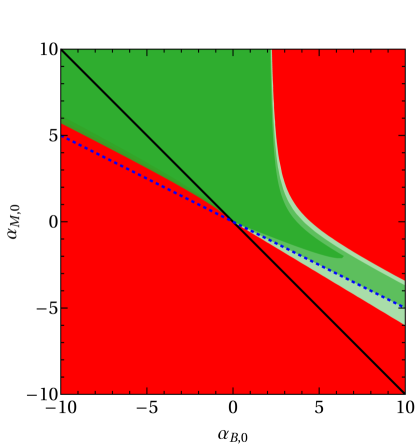
Figure 3: Regions of stability (levels of green) and gradient instability (red) plotted in the $\alpha_{\_}{B,0}$ and $\alpha_{\_}{M,0}$ plane for $s=1.3$ (dark green), $s=1.5$ (green) and $s=1.7$ (light green). Black solid line corresponds to $f(R)$ theories ($\alpha_{\_}B=-\alpha_{\_}M$), blue dotted line corresponds to No Slip Gravity ($\alpha_{\_}B=-2\,\alpha_{\_}M$).

II.3 CMB B-modes and $\alpha_{\_}M$

While the background expansion affects distance observables, and enters into growth of structure, the property functions affect perturbations in density and velocity, impacting growth of structure and gravitational lensing. However, they do not only affect scalar observables such as density perturbations. The propagation of tensor perturbations – gravitational waves – is affected by $\alpha_{\_}T$, which would modify the speed of propagation, and $\alpha_{\_}M$, which influences the friction term in the propagation equation and hence the evolving amplitude of the gravitational wave. As stated above we set $\alpha_{\_}T=0$, but it is interesting to examine the influence of $\alpha_{\_}M$ on gravitational wave observables.

Since $\alpha_{\_}M$ also affects growth of density perturbations leading to cosmic structure, there is a close connection when $\alpha_{\_}T=0$ between the deviation of gravitational wave propagation from general relativity (in particular the distance to the source of gravitational waves compared to its counterpart electromagnetic distance) and the deviation of growth of structure from general relativity, as first explicitly highlighted in nsg . Here, however, we explore primordial gravitational waves evidenced in cosmic microwave background (CMB) polarization B-modes.

B-mode polarization arises from two contributions, the primordial tensor perturbations on large angular scales and the late time gravitational lensing conversion of E-mode polarization into B-modes on small angular scales. Since the lensing arises from structure in the universe it will be affected by growth deviations induced by $\alpha_{\_}M$ and $\alpha_{\_}B$. However the primordial B-modes will predominantly have the effect of an amplitude change due to $\alpha_{\_}M$.

We use hi_class to calculate the B-mode power spectrum, as well as the lensing deflection power spectrum. For the time dependence of the property functions we use the “proptoscale” option in hi_class (see Table 1 of Zumalacarregui:2016pph ), so $\alpha_{\_}i=\alpha_{\_}{i,0}a^{1}$, i.e. $s=1$.

Figure 4 shows the CMB B-mode polarization power spectrum for several values of $\alpha_{M,0}$ and $\alpha_{\_}{B,0}$ in the stability region of the $s=1$ panel of Fig. 2. The low multipole $\ell\lesssim 10$ (large angular scale) reionization bump is due to primordial gravitational waves (here the inflationary tensor to scalar power ratio is taken to be $r=0.01$) and the high $\ell$ bump peaking at $\ell\approx 1000$ is due to lensing.

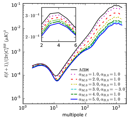
Figure 4: The primordial B-mode spectrum calculated using the property function parametrization of Horndeski models within the hi_class, with time dependence $a^{1}$, for five values of $\alpha_{\_}{M,0}=1,2,3,4,5$, and $\alpha_{\_}{B,0}=1$ or $-3$, $\alpha_{\_}{K,0}=0.001$. The inset zooms in on the low multipoles, showing that only $\alpha_{\_}M$ matters. The tensor-to-scalar ratio $r=0.01$ and all spectra include the effects of gravitational lensing. The $\Lambda$CDM primordial spectrum is given by the solid black curve.

The major effect of $\alpha_{\_}M$ is indeed a shift in amplitude (also see inset). Since $\alpha_{\_}M>0$ increases the friction term in the gravitational wave propagation, it decreases the gravitational wave amplitude, and hence B-mode power. Since $\alpha_{\_}B$ does not affect the gravitational wave propagation it leaves unchanged the B-modes at $\ell\lesssim 10$, but it does enter into the growth of scalar density perturbations responsible for lensing at higher multipoles.

III No Slip Gravity and $f(R)$ Gravity

To understand better, and confirm, the numerical results on stability we consider two specific theories of modified gravity. These will present one dimensional cuts through the $\alpha_{\_}M$–$\alpha_{\_}B$ space. One is $f(R)$ gravity, which imposes the relation $\alpha_{\_}B=-\alpha_{\_}M$, and the other is No Slip Gravity nsg , with the relation $\alpha_{\_}B=-2\,\alpha_{\_}M$. For each of these we need parametrize only one function, which we take to be $\alpha_{\_}M(a)$.

Proceeding along the lines of the previous section, we here adopt

$$\alpha_{\_}M=\alpha_{M,0}\,a^{s}\ .$$ (3)

(The next sections consider further forms.) The analysis is particularly simple for No Slip Gravity as there the stability condition is simply

$$(H\alpha_{\_}M)\,\dot{}\leq 0\qquad{\rm or}\qquad\frac{d(H\alpha_{\_}M)}{da}\leq 0\ .$$ (4)

This then becomes

$$\alpha_{M,0}\,\left[(2s-3)\Omega_{m}a^{-3}+2s(1-\Omega_{m})\right]\leq 0\ ,$$ (5)

where we ignore radiation. We can readily define three cases:

1. $s>3/2$: Stable for $\alpha_{M,0}<0$.

2. $s<3\Omega_{m}/2$: Stable for $\alpha_{M,0}>0$.

3. $3\Omega_{m}/2<s<3/2$: Unstable at some point in $a=[0,1]$.

This agrees with the dotted line in Fig. 2 representing the No Slip Gravity condition $\alpha_{\_}B=-2\alpha_{\_}M$ (note $\alpha_{M,0}=0$ is just general relativity).

For $f(R)$ gravity the stability condition in the power law $\alpha_{\_}M(a)$ model reads

$$\alpha_{M,0}\,\left[1-s+\frac{\alpha_{M,0}a^{s}}{2}+\frac{3}{2}\frac{\Omega_{m}a^{-3}}{\Omega_{m}a^{-3}+1-\Omega_{m}}\right]\geq 0\ .$$ (6)

This gives four cases:

1. $s>5/2$: Stable for $\alpha_{M,0}<0$.

2. $0<s<1+3\Omega_{m}/2$: Stable for $\alpha_{M,0}>0$.

3. $1+3\Omega_{m}/2<s<5/2$: Necessary but not sufficient condition for stability is $\alpha_{M,0}>2[s-(1+3\Omega_{m}/2)]$.

4. $s=0$: Stable for $\alpha_{M,0}>0$ and $\alpha_{M,0}<-5$.

This agrees with the solid line in Fig. 2 representing the $f(R)$ gravity condition $\alpha_{\_}B=-\alpha_{\_}M$. (Note that $s=2$ requires $\alpha_{M,0}>1.11$; the exact stability condition for case F3. is analytic but messy, so we only show the simpler necessary condition.) For $s=0$ we see islands of stability appear that are disconnected from each other. This is an interesting property that we revisit in the next section when considering implicitly stable numerical parametrizations.

There is physical motivation for these two theories, while there is not in general for ones with arbitrary $\alpha_{\_}B=-r\alpha_{\_}M$. However, we can use such a relation to show that:

1. $s>3/2$: Stable for $\alpha_{M,0}>0$ when $r<4/(2s-1)$, for $\alpha_{M,0}<0$ when $4/(2s-1)<r<2$.

2. $s<3/2$: Stable for $\alpha_{M,0}>0$ when $r<2/(1+s-3\Omega_{m}/2)$, unstable for $\alpha_{M,0}<0$.

3. $r<0$: Unstable.

It is interesting to note that $\alpha_{\_}B=-2\alpha_{\_}M$, i.e. No Slip Gravity, is a bounding model in the first case above.

For the two physical theories we now consider the forms of the sound speed $c_{\_}s$ that these stable solutions represent. Figure 5 and Figure 6 show $c_{\_}s(a)$ for various stable power law forms of No Slip Gravity, for $\alpha_{M,0}>0$ and $\alpha_{M,0}<0$ respectively. Note that $c_{\_}s^{2}\propto 1/|\alpha_{M,0}|$ so all the curves simply scale by this relation. At high redshift, $a\ll 1$, the sound speed increases as $c_{\_}s^{2}\sim a^{-s}$, except for the bounding stability case $s=3/2$ and of course $s=0$. (This holds when $\alpha_{\_}K\ll\alpha_{\_}B^{2}$. Otherwise, $c_{\_}s^{2}(a\ll 1)$ becomes of order $\alpha_{\_}M/\alpha_{\_}K$, which may go to a constant in the early universe. If $\alpha_{\_}K/\alpha_{\_}M\lesssim 0.1$ the figures we plot are only significantly affected for high $c_{\_}s$ outside the range shown, so for simplicity we keep $\alpha_{\_}K=0$. When $\alpha_{\_}K$ gives a qualitative difference we will discuss it.)

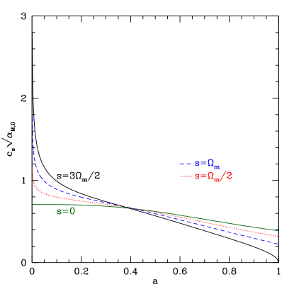
Figure 5: The sound speed $c_{\_}s(a)$ is plotted vs scale factor for four cases of No Slip Gravity with $\alpha_{\_}M=\alpha_{M,0}a^{s}$ and $\alpha_{M,0}>0$. The upper limit of stability is $s=3\Omega_{m}/2$. We take $\Omega_{m}=0.3$.

Figure 6: The sound speed $c_{\_}s(a)$ is plotted vs scale factor for four cases of No Slip Gravity with $\alpha_{\_}M=\alpha_{M,0}a^{s}$ and $\alpha_{M,0}<0$. The lower limit of stability is $s=3/2$.

For $f(R)$ gravity the sound speed behavior is qualitatively similar. Figure 7 illustrates the time dependence for the low $s$ stability range of cases F2. and F4.. Note the similar increase at high redshift. Now the sound speed does not scale simply with $\alpha_{M,0}$ so we plot two different values for each $s$.

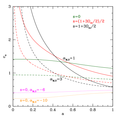
Figure 7: The sound speed $c_{\_}s(a)$ is plotted vs scale factor for the two low $s$ cases of $f(R)$ gravity with $\alpha_{\_}M=\alpha_{M,0}a^{s}$. Note the $s=0$ case allows both positive and some negative values of $\alpha_{M,0}$.

The higher $s$ stability ranges of $f(R)$ cases F1.  and F3. are shown in Figure 8. The behavior is qualitatively similar, where $c_{\_}s^{2}$ grows as $a^{-s}$ at high redshift, except for the bounding stability case of $s=5/2$.

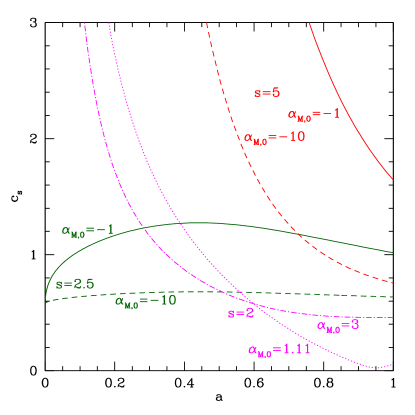
Figure 8: The sound speed $c_{\_}s(a)$ is plotted vs scale factor for the two high $s$ cases of $f(R)$ gravity with $\alpha_{\_}M=\alpha_{M,0}a^{s}$.

IV Starting from Stability

Recently, Kennedy:2018gtx proposed the intriguing idea that rather than scanning through the property function space to check stability conditions, one rewrite the conditions $\alpha=\alpha_{\_}K+(3/2)\alpha_{\_}B^{2}\geq 0$ and $c_{\_}s^{2}\geq 0$ as a differential equation for $\alpha_{\_}B$. That is, for any input $\alpha_{\_}M$ (or the Planck mass $M_{\_}\star$ directly) and $c_{\_}s^{2}>0$ one would obtain $\alpha_{\_}B$ such that the pair ($\alpha_{\_}M,\alpha_{\_}B$) described a stable theory. This is an attractive feature, and furthermore one might hope that one has better guidance on priors for $c_{\_}s$ (at least its magnitude if not time dependence) than for $\alpha_{\_}i$.

The differential equation, whose solution $\alpha_{\_}B(a)$ gives a guaranteed stable system, is

$$\alpha^{\prime}_{\_}B=\alpha c_{\_}s^{2}-\left(1-\frac{\alpha_{\_}B}{2}\right)(2\alpha_{\_}M+\alpha_{\_}B)-\frac{\alpha_{\_}B}{2H^{2}}\left(H^{2}\right)^{\prime}\ ,$$ (7)

where a prime denotes $d/d\ln a$. Note that we use the convention of Bellini:2014fua , which differs from Kennedy:2018gtx by a factor $-2$ in $\alpha_{\_}B$. While Kennedy:2018gtx defines an auxiliary variable $B$ such that $B^{\prime}/B=1+\alpha_{\_}B$ to obtain a second order differential equation (mathematically guaranteeing a real solution), this does not seem to yield any practical advantage so we keep the first order differential equation.

This approach requires parametrization of $\alpha_{\_}M$ (or $M^{2}_{\_}\star$), and adds parametrization of $\alpha$ and $c_{\_}s^{2}$, and an initial condition on $\alpha_{\_}B$ (vs parametrization of $\alpha_{\_}B$, and $\alpha_{\_}K$ if desired, in the standard approach). One might hope to have better intuition on a parametrization for $c_{\_}s^{2}$ than for $\alpha_{\_}i$, but it is not obvious exactly how this would follow from some physical motivation (other than $c_{\_}s^{2}\geq 0$). Implementing this approach requires adding a differential equation (to determine $\alpha_{\_}B$) versus the standard algebraic check of the positivity of $c_{\_}s^{2}$, possibly adding computation time. From Figure 2 we see that the stability region in $\alpha_{\_}M$–$\alpha_{\_}B$ space is not a particularly small fraction of the whole area, so the standard algebraic stability check should not cost more than a factor of a few in a uniform scan.

To test these effects, we track the computational time required by the two approaches. In the standard approach, we uniformly scan over $\alpha_{M,0}$ and $\alpha_{\_}{B,0}$, check stability at $10^{4}$ redshifts from the early to late universe, and calculate the time required to obtain 1000 stable cases. In the stability approach we do not have to check stability – it is guaranteed – but we do have to solve the differential equation to determine $\alpha_{\_}B(a)$. We input $\alpha_{\_}M(a)$ and $c_{\_}s^{2}(a)$ then evaluate $\alpha_{\_}B(a)$ at $10^{4}$ redshifts, and change the amplitude of $c_{\_}s^{2}$ at the present to obtain 1000 cases, again calculating the computational time. (Note that to minimize time we have not added further parameters to describe $\alpha$, but keep it fixed, just as we do with $\alpha_{\_}K$ in the standard approach.)

In both cases we take the input functions to vary as $a^{s}$, with $s=1$; this gives the greatest disadvantage to the standard approach, since from Fig. 2 we see the smallest area of the parameter space is stable, 22%. Despite this, the computational efficiencies are not significantly different (to generate 1000 cases we find the standard approach is 7% quicker).

There is another important aspect. While the stability approach has the desirable property that it is pure in obtaining stability, it is not complete in the following sense. For a given parametrization of $c_{\_}s^{2}$, $\alpha$, and $\alpha_{\_}M$ one obtains a determined $\alpha_{\_}B$; this $\alpha_{\_}B$ will generally not have a strict proportionality to the chosen $\alpha_{\_}M$, i.e. $\alpha_{\_}B=-r\alpha_{\_}M$, and so physical models that enforce this, such as $f(R)$ gravity and No Slip Gravity, may be left out for at least some choices of parameter space.

We pursue the extent of such restrictions further in the next section where we consider observational implications for parametrizations.

V Observational Considerations

Two observational and physical considerations that we may want to take into account are that at early times we want the predictions to match general relativity, due to its success for primordial nucleosynthesis and the cosmic microwave background, and that at late times we may want the possibility of a de Sitter state to match the assumed background expansion history. These have particular implications for the property functions.

In general, we want the $\alpha_{\_}i$ property functions to vanish at early times to give general relativity in the early universe, and $\alpha_{\_}M$ to vanish at late times if we desire a de Sitter state (since it is a running of the Planck mass). The other property functions, and the sound speed, should go to constants in the de Sitter limit. Thus, rather than a power law form, these would have more of a “hill” form. To see what this implies for the sound speed, consider the $\alpha_{\_}M(a)$ hill form used for No Slip Gravity in nsg ,

$$\alpha_{\_}M(a) = A\,\left[1-\tanh^{2}\left(\frac{\tau}{2}\ln\frac{a}{a_{\_}t}\right)\right]$$ (8)

$$= 4A\,\frac{(a/a_{\_}t)^{\tau}}{[(a/a_{\_}t)^{\tau}+1]^{2}}\ ,$$ (9)

where $A$ is the amplitude, $\tau$ the steepness, and $a_{\_}t$ the location of the hill. This form (within No Slip Gravity) is guaranteed stable within the appropriate range ($\tau\leq 3/2$). Figure 9 illustrates the resulting $c_{\_}s(a)$.

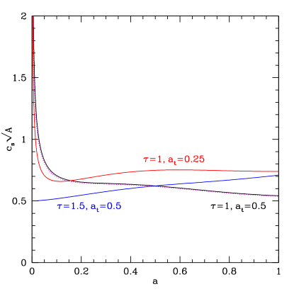
Figure 9: The sound speed $c_{\_}s(a)$ is plotted vs scale factor for the “hill” form in No Slip Gravity, for different values of $\tau$ and $a_{\_}t$. The dotted, magenta curve uses the same parameters as the solid, black curve, but with $\alpha_{\_}K=0.1\alpha_{\_}M$; the function $\alpha_{\_}K$ has little effect within the region of interest.

We find that $c_{\_}s$ is fairly well behaved except at early times when it grows as $a^{-\tau/2}$. The boundary stability case of $\tau=3/2$ is an exception to this divergence; there $c_{\_}s(a\ll 1)\to 1/(2\sqrt{A})$. Note that in general $c_{\_}s(a)\propto A^{-1/2}$, where $A$ is the amplitude $\alpha_{\_}M(a_{\_}t)$. The amplitude today is given by $\alpha_{M,0}=4A/(a_{\_}t^{\tau/2}+a_{\_}t^{-\tau/2})^{2}$, or $(8/9)A$ for $\tau=1$ and $a_{\_}t=0.5$.

However, these early time behaviors assume $\alpha_{\_}K\ll\alpha_{\_}B^{2}$, so let us examine when this does not hold. The dotted, magenta curve in Fig. 9 sets $\alpha_{\_}K=0.1\alpha_{\_}M$, so that it is not zero, and $\alpha_{\_}K\gg\alpha_{\_}B^{2}$ at early times. However, over late times relevant to observational tests of gravity, $\alpha_{\_}K$ makes little difference.

That is the basic conclusion, but let’s go into some further detail. As all the property functions become small in the approach to general relativity at early times, we can write

$$c_{\_}s^{2}\to\frac{2\alpha_{\_}M+\alpha_{\_}B}{\alpha_{\_}K}+\frac{\alpha_{\_}B}{\alpha_{\_}K}\frac{d\ln\alpha_{\_}B}{d\ln a}\ .$$ (10)

In many theories all the property functions will become proportional to each other (possibly with proportionality constant of zero) 1512.06180 ; 1607.03113 , and further evolve as power laws of the scale factor. In this case we see from Eq. (10) that at very early times the sound speed approaches a constant. Note that in No Slip Gravity the first term in Eq. (10) vanishes. If $\alpha_{\_}B\sim a^{3(1+w_{\_}b)}$ at early times, where $w_{\_}b$ is the background equation of state (e.g. 1/3 for radiation domination), then $c_{\_}s^{2}\to(3/2)(1+w_{\_}b)\alpha_{\_}B/\alpha_{\_}K$ for No Slip Gravity and $c_{\_}s^{2}\to(1/2)(1+3w_{\_}b)\alpha_{\_}B/\alpha_{\_}K$ for $f(R)$ gravity.

Now considering late times, if the universe goes to a de Sitter state, then all time derivatives, e.g. $\dot{H}$ and $\alpha^{\prime}_{\_}B$, vanish. This holds as well for $\alpha_{\_}M=d\ln M^{2}_{\_}\star/d\ln a\to 0$. Thus we have

$$c_{\_}s^{2}\to\frac{\alpha_{\_}B\,(1-\alpha_{\_}B/2)}{\alpha_{\_}K+(3/2)\alpha_{\_}B^{2}}\ .$$ (11)

All $\alpha_{\_}i$ should go to constants in the de Sitter state, and so the sound speed also goes to a constant. If the gravity theory has a relation $\alpha_{\_}B=-r\alpha_{\_}M$, then since $\alpha_{\_}M\to 0$ then $\alpha_{\_}B$ also vanishes and $c_{\_}s\to 0$. In particular, this holds for No Slip Gravity and $f(R)$ gravity.

Returning to the stability approach and its required parametrization of the sound speed, let us consider the two theories of $f(R)$ and No Slip Gravity to see what are the forms of $c_{\_}s^{2}(a)$ associated with them. This will give an idea for how straightforward it might be to start with a parametrization of sound speed. We can avoid the issue of $\alpha_{\_}K$ within the differential equation method by parametrizing the combination $q\equiv\alpha c_{\_}s^{2}$ which is all that enters, rather than $\alpha$ and $c_{\_}s^{2}$ separately. We still need to parametrize $\alpha_{\_}M$ or $M^{2}_{\_}\star$. For $f(R)$ we can evaluate $q$ using $\alpha_{\_}B=-\alpha_{\_}M$, and for No Slip Gravity using $\alpha_{\_}B=-2\alpha_{\_}M$; for both we use the hill form of $\alpha_{\_}M(a)$. Figure 10 shows the derived $q(a)$.

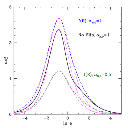
Figure 10: The combined sound speed $q\equiv\alpha c^{2}_{\_}s(a)$ is plotted vs log scale factor for $f(R)$ gravity (dashed, blue curve for $\alpha_{M,0}=1$ and dotted, dark green curve for $\alpha_{M,0}=0.5$) and No Slip Gravity (solid, black curve) with $\alpha_{\_}M(a)$ given by the hill form. The dot dashed, magenta curves for each case give a fit to $q(a)$, using a similar hill functional form. Note for No Slip Gravity that $q$ simply scales with $\alpha_{M,0}$, while there is mild additional dependence for $f(R)$ gravity.

These cases appear more tractable to parametrization than those from the previous power law cases. But that functional sensitivity means it is not clear that one can fruitfully employ one simple general form for $c_{\_}s^{2}(a)$ in the stability approach and capture variations in $\alpha_{\_}i$. Nevertheless, let us attempt to go one step further, parametrizing the derived $q(a)$ from a true input theory, as in Fig. 10, and seeing if the stability approach then accurately reconstructs the true theory. From Fig. 10 a hill form, shown by the dot-dashed, magenta curves, appears a reasonable approximation to $q$, at least over the range of most observational interest .

We then use the same input function $\alpha_{\_}M(a)$ as in Fig. 10. Furthermore, we take initial conditions on $\alpha_{\_}B$ such that it has the characteristic $\alpha_{\_}{B,i}=-2\alpha_{\_}{M,i}$ of a No Slip Gravity theory or $\alpha_{\_}{B,i}=-\alpha_{\_}{M,i}$ of $f(R)$ gravity. We use these as inputs to solving the differential equation for $\alpha_{\_}B(a)$ in the stability approach. Figure 11 shows the results.

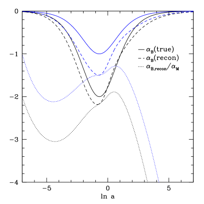
Figure 11: Approximating the exact solution for $q$ by a hill form, i.e. a reasonable parametrization attempt, does not reconstruct accurately the input gravity theories. Solid curves are the true $\alpha_{\_}B$ for the input No Slip Gravity (dark black) or $f(R)$ gravity (light blue) theories, while dashed curves show the reconstruction based on using parameters that match the $\alpha c_{\_}s^{2}$ curves in Fig. 10. Dotted curves show the ratio $\alpha_{\_}{B,recon}/\alpha_{\_}{M,input}$; if the reconstruction were accurate then these curves should be horizontal at $-2$ for No Slip Gravity and at $-1$ for $f(R)$ gravity. While $\alpha_{\_}B$ may look of a similar hill form as $\alpha_{\_}M$, the No Slip Gravity relation $\alpha_{\_}B=-2\alpha_{\_}M$ or the $f(R)$ gravity relation $\alpha_{\_}B=-\alpha_{\_}M$ is not followed.

The reconstructed $\alpha_{\_}B(a)$ do not closely match the input truth. While $\alpha_{\_}B$ is roughly a hill form as it should be in mirroring $\alpha_{\_}M$, the amplitude and width are larger than they should be. Moreover, we do not recover the class of gravity theory, i.e. the ratio $\alpha_{\_}B/\alpha_{\_}M$ that are the characteristics of No Slip Gravity and $f(R)$ gravity. These key ratios are, in the reconstruction, neither constant nor centered on the right values for the two theories.

Finally, if one propagates the reconstruction to the modified Poisson equation gravitational strengths, $G_{\rm matter}$ and $G_{\rm light}$, one breaks characteristics such as $G_{\rm matter}=G_{\rm light}$ for No Slip Gravity and also obtains pathological results at some redshifts as their denominators vanish due to inaccuracy of the reconstructed $\alpha_{\_}B$ and $\alpha^{\prime}_{\_}B$. (See 1712.00444 for a different study of the impact of stability on the gravitational strengths.) This is of particular concern since they are closely related to observables. It appears that even modestly inexact parametrization of the sound speed can lose significant information on the nature of modified gravity.

If even these two viable theories, much less complicated than many Horndeski theories, cannot easily parametrize the essential element, $q$, entering the stability approach, and give rise to accurate physical interpretation, then the utility of property function (and sound speed) parametrization seems to lack robustness. We discuss an alternative in the Conclusions.

VI Conclusions

Modified gravity as an explanation for cosmic acceleration is a highly attractive concept, and has been connected to the observations in an increasingly sophisticated manner in recent years. If one wants to extract general physical characteristics of the theory, rather than working within one specific theory (with a particular functional form assumed, and particular values for the parameters assumed), then approaches such as effective field theory or property functions or modified Poisson equations are quite useful.

However, these all contain functions that themselves need to be parametrized. Even before engaging in detailed calculations of such parametrized theories one must check that the theory is sound: lacking ghosts and instability. We examined in some detail the relation between the functional parametrization in the property function approach and the stability of the theory: the relation is not trivial. In particular, we showed how the stability evolves with redshift, picking out different regions of parameter space that can have complex structure (see Fig. 1). The final allowable stable part of parameter space is the intersection of stability for all redshifts. This can exhibit disconnected islands and also shows significant sensitivity to the time dependent form assumed for the property functions, even for the case where only two property functions contribute. Such sensitivity raises questions about the utility of the property function (or EFT) approach to give robust, general conclusions about modified gravity.

Exploring this further, we considered a power law time dependence and studied the change in stability region as a function of power law index $s$. We derived various analytic expressions for the stability conditions and related them to two modified gravity theories: $f(R)$ gravity and No Slip Gravity. No Slip Gravity has the interesting property that it is a bounding theory: no theory that lies beyond No Slip Gravity in the relation $\alpha_{\_}B=-r\alpha_{\_}M$, i.e. with $r>2$, is stable for $s>3/2$ for all $\alpha_{M,0}<0$. The property function $\alpha_{\_}M$ is particularly interesting since it affects gravitational wave propagation, as well as density perturbations. We exhibited its effect on CMB B-mode polarization from primordial gravitational waves (and late time lensing), illustrating how it scales the power (as it does for late universe gravitational waves as well).

A derived property from the property functions is the sound speed of scalar perturbations. We examined the implications of various parametrizations of the property functions on the sound speed, finding a great diversity in its behaviors – power law dependence giving large $c_{\_}s$ at early times, bounded but nonmonotonic variation, both concave and convex variation – all within the stability criterion and coming from simple power law time dependence of the property functions. This is directly relevant to the attractive idea by Kennedy:2018gtx that one could start with enforcing stability by choosing a positive sound speed and then deriving the form of the property function $\alpha_{\_}B(a)$ preserving stability. That is, since $c_{\_}s$ is a function of $\alpha_{\_}M$ and $\alpha_{\_}B$, one can choose any two and determine the third function. However, our finding that simple $\alpha_{\_}i$’s give complicated $c_{\_}s$ casts some doubt on the approach of parametrizing $c_{\_}s(a)$.

To explore this, we chose several forms of $c_{\_}s(a)$ (and $\alpha_{\_}M(a)$) and calculated the resulting $\alpha_{\_}B(a)$. We found that even if we chose a form $c_{\_}s(a)$ close to that predicted from a full theory such as $f(R)$ or No Slip Gravity, the reconstructed $\alpha_{\_}B$ and overall modified gravity was not faithful to the original. It broke essential physical characteristics such as injecting slip into No Slip Gravity or breaking the relation $\alpha_{\_}B=-\alpha_{\_}M$ in $f(R)$ gravity. Moreover, this stability approach was pure but not complete – it did indeed guarantee stability but it did not (with reasonable guesses for the parametrized function $c_{\_}s(a)$) generate standard theories such as $f(R)$ gravity.

Another relevant question is whether this stability approach is efficient. Removing the need for a stability check in the Boltzmann code saves computational time, but adding an extra differential equation to solve (and possibly increasing the overall number of parameters because one may have to account for $\alpha$, or $\alpha_{\_}K$, while it can mostly be ignored in the standard approach) compared to the standard approach of parametrizing $\alpha_{\_}B$ and $\alpha_{\_}M$ can cost time. We checked this and found there was no significant time savings from the stability approach, even when it did not involve an increased number of parameters.

Finally, we investigated the impact of observational constraints on allowable parametrizations. One would like to impose that general relativity is restored in the early universe, so all the $\alpha_{\_}i$ go to zero. We explored the resulting implications on the sound speed. Similarly, one might look for a de Sitter state in the asymptotic future, and we discussed its implications on the property functions and sound speed. A useful parametrization that encompasses both these conditions is the “hill” form, and we compute $c_{\_}s$ and $\alpha_{\_}B$ in this case. We motivated use of the combination $q=\alpha c_{\_}s^{2}$ which enters the equation for $\alpha_{\_}B$, and showed this can be reasonably fit by the hill form, and in turn the reconstructed $\alpha_{\_}B$ looks qualitatively, if not quantitatively, similar to the input truth.

However, we demonstrated that even small inaccuracies in the reconstructed $\alpha_{\_}B$, from residuals of the parametrization of the sound speed, can give rise to significant physical flaws. The denominators of the gravitational strengths $G_{\rm matter}$ and $G_{\rm light}$ can spuriously pass through zero, giving pathologies. Combined with the lack of fidelity in preserving physical characteristics of known theories such as $f(R)$ and No Slip Gravity, and indeed the difficulty including them using straightforward parametrizations of the sound speed, this means that parametrization in terms of property functions or EFT is highly nontrivial, notwithstanding stability considerations.

Parametrizations from the theory side, while undeniably attractive, unfortunately are found to be subject to issues of functional sensitivity and lack of robustness. However, there is a reasonable solution by moving closer to the observables. The gravitational strengths $G_{\rm matter}$ and $G_{\rm light}$ entering the modified Poisson equations, directly related to growth of matter structure and light deflection, have been demonstrated to give robust and highly accurate descriptions of the observables, as well as key indicators to theory characteristics Denissenya:2017thl ; Denissenya:2017uuc . Such simple, model independent parametrizations as binning in redshift of these functions can be a highly useful first step in uncovering signatures of modified gravity.

- (1) E. Bellini and I. Sawicki, Maximal freedom at minimum cost: linear large-scale structure in general modifications of gravity, JCAP 1407, 050 (2014) [arXiv:1404.3713]
- (2) E. V. Linder, G. Sengör and S. Watson, Is the Effective Field Theory of Dark Energy Effective?, JCAP 1605, 053 (2016) [arXiv:1512.06180]
- (3) E. V. Linder, Challenges in connecting modified gravity theory and observations, Phys. Rev. D 95, 023518 (2017) [arXiv:1607.03113]
- (4) A. de Felice, N. Frusciante, G. Papadomanolakis, A de Sitter limit analysis for dark energy and modified gravity models, Phys. Rev. D 96, 024060 (2017) [arXiv:1705.01960]
- (5) G. Domènech, A. Naruko, M. Sasaki, Cosmological disformal invariance, JCAP 1510, 067 (2015) [arXiv:1505.00174]
- (6) K. Koyama, Cosmological Tests of Modified Gravity, Rept. Prog. Phys. 79, 046902 (2016) [arXiv:1504.04623]
- (7) J. Kennedy, L. Lombriser and A. Taylor, Reconstructing Horndeski theories from phenomenological modified gravity and dark energy models on cosmological scales, arXiv:1804.04582
- (8) E. M. Mueller, W. Percival, E. Linder, S. Alam, G. B. Zhao, A. G. Sánchez, F. Beutler and J. Brinkmann, The clustering of galaxies in the completed SDSS-III Baryon Oscillation Spectroscopic Survey: constraining modified gravity, Mon. Not. Roy. Astron. Soc. 475, 2122 (2018) [arXiv:1612.00812]
- (9) M. Zumalacárregui, E. Bellini, I. Sawicki, J. Lesgourgues and P. G. Ferreira, hiclass: Horndeski in the Cosmic Linear Anisotropy Solving System, JCAP 1708, 019 (2017) [arXiv:1605.06102]
- (10) M. Raveri, B. Hu, N. Frusciante and A. Silvestri, Effective Field Theory of Cosmic Acceleration: constraining dark energy with CMB data, Phys. Rev. D 90, 043513 (2014) [arXiv:1405.1022]
- (11) B.P. Abbott et al., Gravitational Waves and Gamma-Rays from a Binary Neutron Star Merger: GW170817 and GRB 170817A, Astrophys. J. Lett. 848, L13 (2017) [arXiv:1710.05834]
- (12) L. Amendola, D. Bettoni, G. Domènech, A.R. Gomes, Doppelgänger dark energy: modified gravity with non-universal couplings after GW170817, JCAP 1806, 029 (2018) [arXiv:1803.06368]
- (13) R.A. Battye, F. Pace, D. Trinh, Gravitational wave constraints on dark sector models, Phys. Rev. D 98, 023504 (2018) [arXiv:1802.09447]
- (14) C. de Rham, S. Melville, Gravitational Rainbows: LIGO and Dark Energy at its Cutoff, arXiv:1806.09417
- (15) S. Peirone, M. Martinelli, M. Raveri and A. Silvestri, Impact of theoretical priors in cosmological analyses: the case of single field quintessence, Phys. Rev. D 96, 063524 (2017) [arXiv:1702.06526]
- (16) M. Raveri, P. Bull, A. Silvestri, L. Pogosian, Priors on the effective Dark Energy equation of state in scalar-tensor theories, Phys. Rev. D 96, 083509 (2017) [arXiv:1703.05297]
- (17) E. V. Linder, No Slip Gravity, JCAP 1803, 005 (2018) [arXiv:1801.01503]
- (18) S. Peirone, K. Koyama, L. Pogosian, M. Raveri, A. Silvestri, Large-scale structure phenomenology of viable Horndeski theories, Phys. Rev. D 97, 043519 (2018) [arXiv:1712.00444]
- (19) M. Denissenya and E. V. Linder, Cosmic Growth Signatures of Modified Gravitational Strength, JCAP 1706, 030 (2017) [arXiv:1703.00917]
- (20) M. Denissenya and E. V. Linder, Subpercent Accurate Fitting of Modified Gravity Growth, JCAP 1711, 052 (2017) [arXiv:1709.08709]