Positivity bounds on vector boson scattering at the LHC

Abstract

Weak vector boson scattering (VBS) is a sensitive probe of new physics effects in the electroweak symmetry breaking. Currently, experimental results at the LHC are interpreted in the effective field theory approach, where possible deviations from the Standard Model in the quartic-gauge-boson couplings are often described by 18 dimension-8 operators. By assuming that a UV completion exists, we derive a new set of theoretical constraints on the coefficients of these operators, i.e. certain combinations of coefficients must be positive. These constraints imply that the current effective approach to VBS has a large redundancy: only about $2\%$ of the full parameter space leads to a UV completion. By excluding the remaining unphysical region of the parameter space, these constraints provide guidance for future VBS studies and measurements.

Introduction.— After the discovery of the Higgs boson Aad:2012tfa ; Chatrchyan:2012xdj , the focus of particle physics has turned to the mechanism of electroweak symmetry breaking and beyond. At the Large Hadron Collider (LHC), vector boson scattering (VBS) is among the processes most sensitive to the electroweak and the Higgs sectors. In the Standard Model (SM), Feynman amplitudes for longitudinally polarized weak bosons individually grow with energy, but cancellations among diagrams involving quartic gauge boson couplings (QGC), trilinear gauge boson couplings (TGC), and Higgs exchange occur, and lead to a total amplitude that does not grow at large energies. If modifications from physics beyond the Standard Model (BSM) exist, they are likely to spoil these cancellations and lead to sizable cross section increases.

VBS processes at the LHC can be embedded in partonic processes $qq\to VVqq$, where $q$ is a light quark. Both ATLAS and CMS experiments have extensively studied this kind of signatures, and the effort will continue with future runs of LHC. Absent clear hints for BSM theories, these studies are based on a bottom-up effective field theory (EFT) approach—the SMEFT Weinberg:1978kz ; Buchmuller:1985jz ; Leung:1984ni . In this approach, deviations in QGC independent of TGC are captured by 18 dimension-8 effective operators, assuming that TGC and Higgs couplings are constrained by other processes with better experimental accuracies, such as diboson and Higgs on-shell measurements. With this assumption, VBS measurements at the LHC have been conveniently interpreted as constraints on these operator coefficients, see, for example, Sirunyan:2017ret ; Sirunyan:2019ksz ; Sirunyan:2017fvv ; Sirunyan:2019der ; CMS:2019iuv for some recent results, and cmstwiki for a compilation of existing experimental limits on QGC coefficients. These constraints in turn can be matched to a variety of BSM theories. (See, for instance, Fleper:2016frz ; Brass:2018hfw ; Giudice:2003tu ; Giudice:1998ck ; Han:1998sg ; Hewett:1998sn ; Liu:2016idz ; Ellis:2017edi ; Davila:2013wba and references therein.) The recent high-luminosity and high-energy LHC projection has shown that future sensitivity on dimension-8 QGC operators at the LHC can go beyond the TeV scale Azzi:2019yne .

However, in order to admit an ultra-violet (UV) completion, QGC operator coefficients cannot take arbitrary values. Recently, a novel approach has been developed to set theoretical bounds on the Wilson coefficients of a generic EFT that can be UV completed. Going under the name of positivity bounds, this approach only requires a minimum set of assumptions, which are nothing but the cherished fundamental principles of quantum field theory such as unitarity, Lorentz invariance, locality, and causality/analyticity of scattering amplitudes. Using the dispersion relation of the amplitude and the optical theorem, Ref. Adams:2006sv established a positivity bound in the forward scattering limit of 2-to-2 scattering (see also Pham:1985cr ; Pennington:1994kc ; Ananthanarayan:1994hf ; Comellas:1995hq ; Dita:1998mh for earlier discussions and applications in QCD). The bound can be computed completely within the low energy EFT and implies that a certain combination of Wilson coefficients must be positive. Moreover, thanks to the properties of the partial wave expansion, an infinite series of non-forward $t$ derivative positivity bounds are derived ($t$ being the Mandelstam variable) deRham:2017avq ; deRham:2017zjm (see also Nicolis:2009qm ; Vecchi:2007na ; Manohar:2008tc ; Bellazzini:2014waa for earlier discussions on non-forward positivity bounds and Bellazzini:2016xrt for earlier discussions on the forward positivity bound for particles with spin). These positivity bounds have been used to fruitfully constrain various gravity and particle physics theories (see, e.g., Bellazzini:2015cra ; Cheung:2016yqr ; Bellazzini:2016xrt ; Cheung:2016wjt ; Bellazzini:2017fep ; Bonifacio:2016wcb ; deRham:2017imi ; Bellazzini:2017bkb ; deRham:2018qqo ; Bonifacio:2018vzv ; Bellazzini:2018paj ; Distler:2006if ; Bellazzini:2019xts ).

In this work, we apply this approach to the SMEFT formalism for VBS processes, and derive a whole new set of theoretical constraints on the VBS operators. While no bounds can be derived at $\mathcal{O}(\Lambda^{-2})$ , we show that at $\mathcal{O}(\Lambda^{-4})$ certain sums of a linear combination of the dimension-8 QGC coefficients and a quadratic form of the dimension-6 coefficients must be positive. Because the latter is always negative-definite, a number of positivity constraints can be inferred solely on QGC operators.

These constraints have several features. First, based only on the most fundamental principles of quantum field theory, they are general and model-independent. In addition, they have strong impacts: the currently allowed parameter space spanned by 18 dimension-8 coefficients will be drastically reduced, by almost two orders of magnitude in volume. Finally, they constrain the possible directions in which SM deviations could occur, complementary to the experimental limits. By revealing the physically viable region in the 18-dimensional QGC parameter space, these constraints provide important guidance for future VBS studies. On the other hand, if the experiments observed a parameter region that violates the positivity bounds, it would be a very clear sign of violation of the cherished fundamental principles of modern physics.

Effective operators.— Before deriving the positivity constraints, let us briefly describe the model-independent SMEFT approach to VBS processes. The approach is based on the following expansion of the Lagrangian

$$\mathcal{L}_{\mathrm{EFT}}=\mathcal{L}_{\mathrm{SM}}+\sum_{d>4}\sum_{i}\frac{f_{i}^{(d)}}{\Lambda^{d-4}}O_{i}^{(d)},$$ (1)

where $\Lambda$ is the typical scale of new physics. $f^{(d)}$ are the dimensionless coefficients of the dimension-$d$ effective operators. If the underlying theory is known and weakly coupled, they can be determined by a matching calculation. It can be shown that only even-dimensional operators conserve both baryon and lepton numbers Degrande:2012wf , so we focus on dimension-6 and dimension-8 operators. VBS processes can be affected by TGC, Higgs couplings, and QGC couplings. At dimension-6, modifications to TGC and $HVV$ Higgs couplings could arise Rauch:2016pai . QGC couplings are also generated, but they are fully determined by dimension-6 TGC couplings. At dimension-8, QGC couplings could arise independent of TGC couplings. They are parameterized by 18 dimension-8 operators Eboli:2006wa ; Degrande:2013rea ; Eboli:2016kko .

The unique feature of VBS processes is that they are sensitive to BSM effects that manifest as anomalous QGC couplings. One may worry that this sensitivity is masked by possible contamination from anomalous TGC and/or Higgs couplings. However, if these couplings are present, we may expect to first probe them elsewhere, e.g. in diboson production, vector boson fusion, or Higgs production and decay measurements, which are in general measured with a much better accuracy than VBS. For example, TGC couplings are constrained by $WW$ production at LEP2, which has been measured at the percent level accuracy Schael:2013ita . These constraints are further improved by the LHC data Butter:2016cvz ; Biekotter:2018rhp ; Ellis:2014jta ; Ellis:2018gqa ; Grojean:2018dqj . Higgs coupling measurements at the LHC have reached $\mathcal{O}(10\%)$ level precision, and will continue to improve with the high-luminosity upgrade Azzi:2019yne . While there might still be non-negligible dimension-6 effects in VBS Gomez-Ambrosio:2018pnl , the projected sensitivity to dimension-8 QGC couplings at high-luminosity and high-energy LHC beyond the TeV scale Azzi:2019yne suggests that VBS will continue to be an important channel to look for possible BSM deviations in QGC. While a global SMEFT approach including both dimension-6 and dimension-8 operators would be the most reliable, given the current accuracy level one could assume that dimension-6 effects are well-constrained by other channels, and focus on dimension-8 QGC couplings as a first step. This is the assumptions that is used by the experimental collaborations to set limits on QGC couplings. Given that the goal of this work is to provide theory guidance to experimental analysis, we will adopt the same assumption. We nevertheless emphasize that our main conclusion, i.e. positivity bounds on QGC couplings, are independent of the presence of dimension-6 operators, as we will explain later. Therefore they will continue to be useful for future global fits including dimension-6 effects.

Dimension-8 QGC couplings are described by 18 operators. Conventionally, they are divided into three categories: S-type operators involve only covariant derivatives of the Higgs, M-type operators include a mix of field strengths and covariant derivatives of the Higgs, and T-type operators include only field strengths. We use the convention of Degrande:2013rea that has become standard in this community. The definition of these operators can be found in Eqs. (13)-(31) of Degrande:2013rea ($O_{M,6}$ is redundant Sekulla ), and we also list them in the Appendix. The 18 operator coefficients are denoted as

$$f_{S,0},\ f_{S,1},\ f_{S,2},\ f_{M,0},\ f_{M,1},\ f_{M,2},\ f_{M,3},\ f_{M,4},\ f_{M,5},$$

$$f_{M,7},\ f_{T,0},\ f_{T,1},\ f_{T,2},\ f_{T,5},\ f_{T,6},\ f_{T,7},\ f_{T,8},\ f_{T,9}.$$

A summary of existing experimental constraints on these coefficients can be found in cmstwiki . See also Ref. Green:2016trm for a review of QGC measurements at the LHC and their interpretation in the SMEFT.

Positivity bounds.— The simplest positivity bound can be obtained by considering an elastic scattering amplitude in the forward limit $A(s)=A(s,t=0)$ Adams:2006sv . Thanks to the dispersion relations, optical theorem and Froissart bound Froissart:1961ux , it can be shown that the second derivative of $A(s)$ w.r.t. $s$ is positive, after subtracting contributions from the low energy poles. In the following we shall briefly review the forward limit positivity bound, adapted to the context of VBS. We assume that the contributions from the higher dimensional operators are well approximated by the tree level, which is a reasonable assumption given that perturbativity in EFT is always needed for a valid analysis.

If the UV completion is weakly coupled, the BSM amplitude is usually well approximated by its leading tree level contribution $A_{\rm tr}$, which is analytic and satisfies the Froissart bound. Its BSM part simply comes from one particle exchange between SM currents. We can derive a dispersion relation for $A_{\rm tr}$:

$$~{}~{}~{}~{}f_{\rm tr}(s_{p})\equiv\frac{1}{2\pi i}\oint_{\cal C}\mathrm{d}s\frac{A_{\rm tr}(s)}{(s-s_{p})^{3}}$$ (2)

$$=\int^{\infty}_{\Lambda_{\rm th}^{2}\!+M^{2}}\!\!\frac{\mathrm{d}s}{\pi}\frac{{\rm Im}A_{\rm tr}(s)}{(s+s_{p}\!-\!M^{2})^{3}}+\int^{\infty}_{\Lambda_{\rm th}^{2}}\!\!\frac{\mathrm{d}s}{\pi}\frac{{\rm Im}A_{\rm tr}(s)}{(s-s_{p})^{3}},$$ (3)

where $M^{2}\equiv 2m_{1}^{2}+2m_{2}^{2}$, $m_{1}$ and $m_{2}$ being the masses of the interacting particles, and $\Lambda_{\rm th}(\gg M)$ is the mass of the lightest heavy state. ${\cal C}$ is a contour that encircles all the poles in the low energy EFT and, by analyticity of the $s$ complex plane, can be deformed to run around the $s>\Lambda_{\rm th}^{2}$ and $s<-\Lambda_{\rm th}^{2}$ parts of the real axis and along the infinite semi-circles; the infinite semi-circle contributions vanish due to the Froissart bound, and the discontinuities along the real axis give rise to ${\rm Im}A_{\rm tr}(s,0)$ which is nonzero due to the heavy particle poles. Also we have restricted to crossing symmetric amplitudes for simplicity, and to obtain the first term of Eq. (3) we have made a variable change $s\to M^{2}-s$ and used the crossing symmetry ${\rm Im}A_{\rm tr}(M^{2}-s)={\rm Im}A_{\rm tr}(s)$. By the cutting rules, ${\rm Im}A_{\rm tr}(s)$ can be written as a sum of complete squares of 2-to-1 amplitudes, and thus ${\rm Im}A_{\rm tr}(s)>0$. Therefore we infer that $f_{\rm tr}(s_{p})>0$ for $-\Lambda_{\rm th}^{2}<s_{p}<\Lambda_{\rm th}^{2}$. Due to analyticity of the amplitude in complex $s$ plane, $f_{\rm tr}(s_{p})$ can be calculated within the SMEFT as the second derivative of the effective amplitude $A_{\rm tr}(s)$ with the poles subtracted. Since the SM at tree level makes no contribution to the r.h.s. of Eq. (3), $f_{\rm tr}(s)>0$ directly gives positivity constraints on the Wilson coefficients.

The above argument can be easily generalized to cases where the leading EFT amplitude is matched to the loop amplitude in the full theory, and one can derive positivity for the lowest order $n$-loop BSM contribution to VBS, with the SM contribution removed. In this case, the discontinuity above $\Lambda_{\rm th}$ must come from unitarity cuts that only cut the BSM particles, otherwise this amplitude would match to both tree and loop diagrams in EFT with similar sizes, violating the perturbativity assumption. Using the cutting rules, the discontinuity can be written as a sum of complete squares, thus proving positivity.

For a generic UV completion, consider the full amplitude including the SM contribution. The latter could give a constant contribution to the dispersion relation at one loop. To minimize its impact, we subtract out the branch cuts within $|s|<(\epsilon\Lambda)^{2}$ ($\epsilon\lesssim 1$), where the dominant SM contribution resides. This is done by following the improved positivity deRham:2017imi ; Bellazzini:2016xrt ; deRham:2017xox and defining:

$$B_{\epsilon\Lambda}(s_{p})=A(s_{p})-\int^{+(\epsilon\Lambda)^{2}}_{-(\epsilon\Lambda)^{2}}\frac{\mathrm{d}s}{2\pi i}\frac{{\rm Disc}A(s)}{s-s_{p}},$$ (4)

with $M_{\pm}<\epsilon\Lambda<\Lambda$, $M_{\pm}\equiv m_{1}\pm m_{2}$. This subtracted amplitude has the same discontinuity as $A(s)$ above $(\epsilon\Lambda)^{2}$ and also satisfies the Froissart bound . It is free of branch cuts for $|s|<(\epsilon\Lambda)^{2}$, and thus one can analogously obtain a dispersion relation:

$$f_{\epsilon\Lambda}(s_{p})\equiv\frac{\mathrm{d}^{2}B_{\epsilon\Lambda}(s_{p})}{2\;\mathrm{d}s^{2}}=\left[\int^{-(\epsilon\Lambda)^{2}}_{-\infty}\!\!\!+\!\int_{(\epsilon\Lambda)^{2}}^{\infty}\right]\frac{\mathrm{d}s}{2\pi i}\frac{{\rm Disc}A(s)}{(s-s_{p})^{3}}$$

$$=\int^{\infty}_{\small(\epsilon\Lambda)^{2}+M^{2}}\!\!\!\frac{\mathrm{d}s}{\pi}\frac{{\rm Im}A(s)}{(s+s_{p}\!-\!M^{2})^{3}}+\!\int^{\infty}_{\small(\epsilon\Lambda)^{2}}\!\!\frac{\mathrm{d}s}{\pi}\frac{{\rm Im}A(s)}{(s-s_{p})^{3}}.$$ (5)

Making use of the optical theorem, ${\rm Im}A(s)=[(s-M_{-}^{2})(s-M_{+}^{2})]^{1/2}\sigma_{t}>0$ for $s>M_{+}^{2}$, where $\sigma_{t}$ is the total cross section. So we have $f_{\epsilon\Lambda}(s_{p})>0$ for $-(\epsilon\Lambda)^{2}<s_{p}<(\epsilon\Lambda)^{2}$. Again, by contour deformation, $f_{\epsilon\Lambda}(s_{p})$ can be evaluated within the EFT with the subtraction term in Eq. (4) taken into account. This term does not contain any tree level contribution from the higher dimensional operators, but it removes the dominant impact from the SM loop contribution. The remaining contribution from the SM is then suppressed by $(\epsilon\Lambda)^{-2}$, and can be computed explicitly. The reason behind is that the SM contribution mostly comes from the discontinuity below $\epsilon\Lambda$, while the BSM contribution is from above this scale, so one can choose a $\epsilon\Lambda$ to subtract the dominant SM contribution without losing positivity. In the Appendix we compute the remaining SM contribution in the $\gamma\gamma$ channel and show that it is negligible even comparing with the best experimental sensitivity currently available.

Applications.— Let us first focus on dimension-8 operators. Applying this approach to the scattering amplitudes of VBS in the forward limit yields a set of positivity constraints on QGC coefficients. As an example, we present here the constraint from $ZZ\to ZZ$ scattering:

$$8a_{3}^{2}b_{3}^{2}t_{W}^{4}\left(F_{S,0}+F_{S,1}+F_{S,2}\right)+\left[a_{3}^{2}\left(b_{1}^{2}+b_{2}^{2}\right)\right.$$

$$\left.+\left(a_{1}^{2}+a_{2}^{2}\right)b_{3}^{2}\right]t_{W}^{2}\left(-t_{W}^{4}F_{M,3}+t_{W}^{2}F_{M,5}-2F_{M,1}+F_{M,7}\right)$$

$$+\left[\left(a_{1}b_{1}+a_{2}b_{2}\right){}^{2}+\left(a_{1}^{2}+a_{2}^{2}\right)\left(b_{1}^{2}+b_{2}^{2}\right)\right]\left(2t_{W}^{8}F_{T,9}\right.$$

$$\left.+4t_{W}^{4}F_{T,7}+8F_{T,2}\right)+8\left(a_{1}b_{1}+a_{2}b_{2}\right){}^{2}\left[t_{W}^{4}\left(t_{W}^{4}F_{T,8}\right.\right.$$

$$\left.\left.+2F_{T,5}+2F_{T,6}\right)+4F_{T,0}+4F_{T,1}\right]\geq 0,$$ (6)

where $t_{W}\equiv\tan\theta_{W}$ is the tangent of the weak angle. We have rewritten the coefficients as

$$F_{S,i}\equiv f_{S,i},~{}~{}F_{M,i}\equiv e^{2}f_{M,i},~{}~{}F_{T,i}\equiv e^{4}f_{T,i}.$$ (7)

$a_{i}$ and $b_{i}$ parametrize the polarization vectors of the two $Z$ bosons respectively:

$$\epsilon_{1}^{\mu}=\left(a_{3}{p_{1}}/{m_{Z}},a_{1},a_{2},a_{3}{E_{1}}/{m_{Z}}\right)$$ (8)

$$\epsilon_{2}^{\mu}=\left(b_{3}{p_{2}}/{m_{Z}},b_{1},b_{2},b_{3}{E_{2}}/{m_{Z}}\right),$$ (9)

where real polarizations are used for simplicity. Eq. (6) must hold for all real values of $a_{i}$ and $b_{i}$. Other VBS processes yield similar but independent constraints. The full set of results are given in the Appendix.

Interestingly, including dimension-6 operators does not change our conclusion. If one follows the same approach and considers dimension-6 contributions, it turns out that nontrivial constraints on them can be obtained only at the $(f^{(6)}/\Lambda^{2})^{2}$ level, i.e. from diagrams involving two insertions of operators. They always take the following form:

$$\sum_{i}(-x_{i})\left(\sum_{j}y_{j}f_{j}^{(6)}\right)^{2}\geq 0,\quad x_{i}>0,$$ (10)

i.e. the sum of a set of complete square terms need to be negative. We have checked this for all relevant dimension-6 operators in the Warsaw basis Grzadkowski:2010es . Explicit results are given in the Appendix. Of course, these conditions cannot be satisfied with dimension-6 operators alone. Instead, it tells us that at $\mathcal{O}(\Lambda^{-4})$ the dimension-8 contribution has to come in, with a positive value large enough to flip the sign of the dimension-6 contribution. Therefore, the presence of dimension-6 contributions will only make the dimension-8 positivity constraints stronger. Our conclusion thus holds regardless of the presence of dimension-6 operators.

It is worth mentioning that these constraints are different from bounds derived from partial-wave unitarity Corbett:2014ora ; Corbett:2017qgl , in that they require unitarity of the UV theory, not the low energy effective theory, and additionally require other fundamental principles such as analyticity of the amplitude. In VBS, partial-wave unitarity leads to bounds on the sizes of $f^{(6)}/\Lambda^{2}$ or $f^{(8)}/\Lambda^{4}$, while the positivity bounds are on the dimensionless coefficients, and lead to constraints on possible directions of SM deviations. These constraints are always complementary to the unitarity bounds and experimental limits.

Physics implication.— We now describe the physics implications of our positivity constraints on VBS processes.

$f_{S,0}$	$f_{S,1}$	$f_{S,2}$	$f_{M,0}$	$f_{M,1}$	$f_{M,2}$	$f_{M,3}$	$f_{M,4}$	$f_{M,5}$
+	+	+	X	$-$	O	$-$	O	X
$f_{M,7}$	$f_{T,0}$	$f_{T,1}$	$f_{T,2}$	$f_{T,5}$	$f_{T,6}$	$f_{T,7}$	$f_{T,8}$	$f_{T,9}$
+	+	+	+	X	+	X	+	+

Table 1: Positivity constraints on individual VBS operator coefficients. $+/-$ means the coefficient must be non-negative or non-positive. X means only $f=0$ is allowed, and O means no constraints.

First, let us turn on one operator at a time. Most experimental results are presented as limits on individual operators, assuming all others vanish. As shown in cmstwiki , these limits are symmetric or nearly symmetric. In Table 1 we list our positivity constraints on individual operators. We can see that, while $f_{M,2}$ and $f_{M,4}$ are free of such constraints, all other coefficients are bounded at least from one side. This implies that half of the experimentally allowed regions do not lead to a UV completion. In addition, $f_{M,0}$, $f_{M,5}$, $f_{T,5}$ and $f_{T,7}$ cannot individually take any nonzero values. $f_{M,0}$ is forbidden because the same-sign and opposite-sign $WW$ scattering amplitudes give inconsistent constraints, while $f_{M,5}$ is forbidden because $WW$ and $WZ$ scattering amplitudes give inconsistent constraints. Similar situations occur for $f_{T,5}$ and $f_{T,7}$. This implies that no UV theory could generate any of the four coefficients alone. We will show that these conditions can be relaxed once other coefficients are allowed to take nonzero values. However, the one-operator-at-a-time scenario already illustrates that the positivity constraints have drastic impacts on the presentation and interpretation of experimental results.

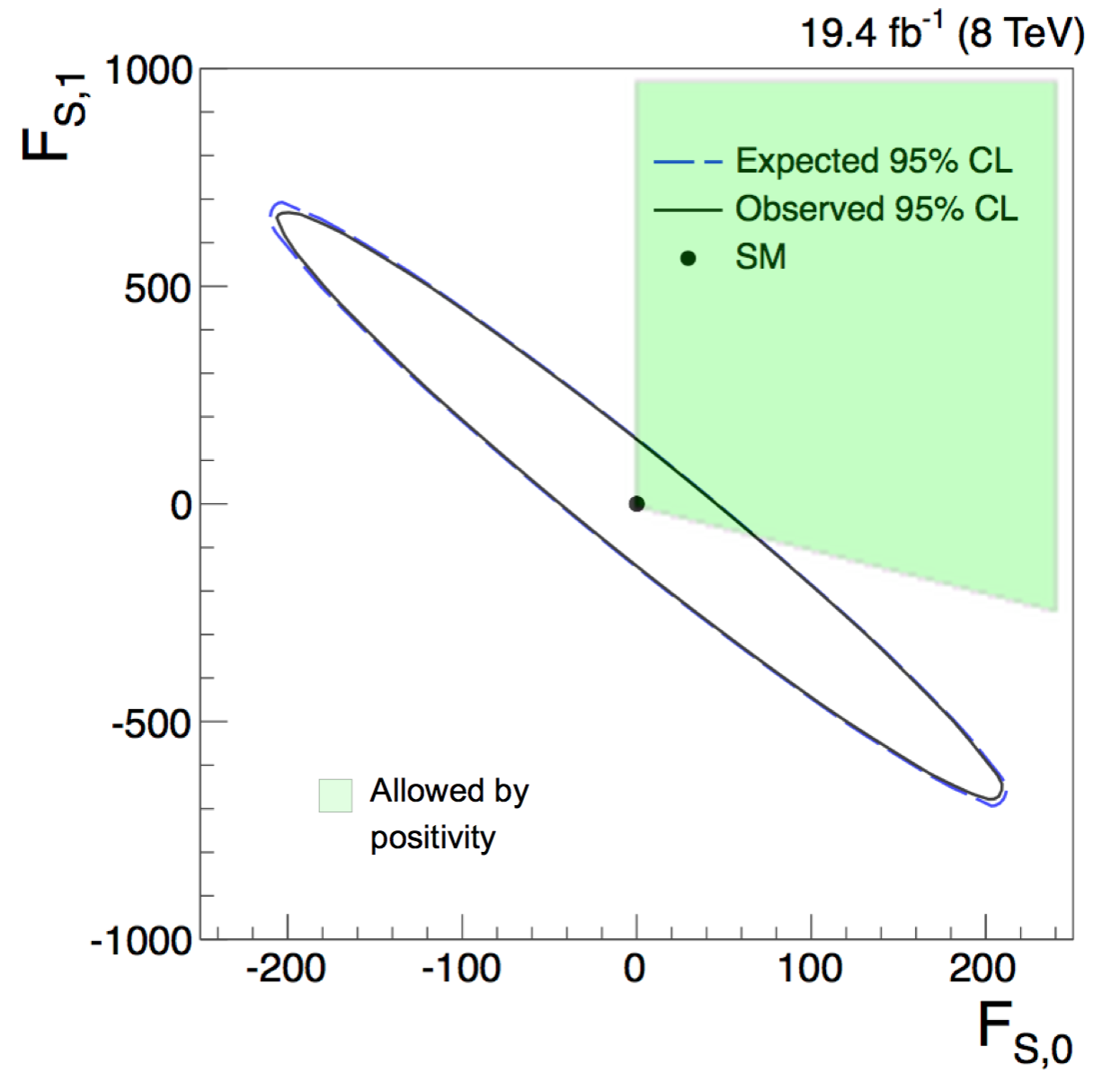
Figure 1: Positivity constraints on $F_{S,0}\equiv f_{S,0}$ and $F_{S,1}\equiv f_{S,0}$, compared with the CMS results Khachatryan:2014sta . The green shaded area is allowed by positivity. A specific combination of $F_{S,0}$ and $F_{S,1}$ roughly rescales the Standard Model distribution, and so the measurement is insensitive to this direction.

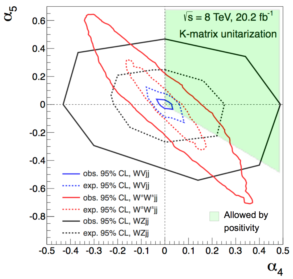
Figure 2: Positivity constraints on $\alpha_{4}$ and $\alpha_{5}$, compared with the ATLAS results Aaboud:2016uuk ; Aaboud:2016ffv ; Aad:2016ett . The green shaded area is allowed by positivity. The difference between the expected limits and the observed ones are due to fluctuations in the observed events.

Now let us turn on two operators simultaneously. Two-operator constraints have been presented by CMS, on coefficients $F_{S,0}\equiv f_{S,0}$ and $F_{S,1}\equiv f_{S,0}$ (see Eq. (7) for relations between the $F$ and $f$ coefficients), and by ATLAS on $\alpha_{4}$ and $\alpha_{5}$. The latter parameters are defined in the nonlinear formulation, but the conversion to the linear case is straightforward Rauch:2016pai :

$$\alpha_{4}=\frac{v^{4}}{16}\frac{f_{S,0}+f_{S,2}}{\Lambda^{4}},\quad\alpha_{5}=\frac{v^{4}}{16}\frac{f_{S,1}}{\Lambda^{4}},$$ (11)

$$\mbox{with}\quad f_{S,0}=f_{S,2}.$$ (12)

In Figures 1 and 2, we overlay our corresponding positivity constraints on top of the two-dimensional contour plots obtained by both experimental groups. We can see that most of the currently allowed areas are excluded. In other words, only a very small fraction of the allowed parameter space could lead to a UV completion.

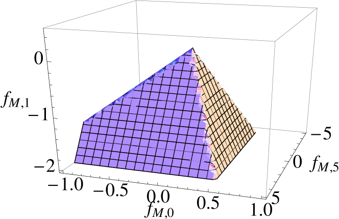
Figure 3: Positivity constraints on $f_{M,0}$, $f_{M,1}$, and $f_{M,5}$.

We are not aware of any constraints assuming three operators are present simultaneously. Nevertheless, for illustration, in Figure 3 we present our constraints on three coefficients, $f_{M,0}$, $f_{M,1}$, and $f_{M,5}$. We can see that the allowed region has the shape of a pyramid. Manifestly, $f_{M,0}$ and $f_{M,5}$ cannot take nonzero values alone, but this is relaxed once $f_{M,1}$ takes a negative value. This is consistent with our previous observation.

Finally, a model-independent SMEFT should always take into account all operators. An interesting question to ask in this case is the following. Suppose future experiments at the LHC and even future colliders will collect sufficient data to derive the global constraints on 18 operators. How large is the impact of the positivity constraints?

To simplify the problem, assume that all 18 operators are constrained in the interval $-\delta<f_{i}<\delta$ without any correlations. The allowed region in the 18-dimensional parameter space will be approximately a 18-ball with radius $\delta$. The fraction of its volume that satisfies all positivity constraints is independent of $\delta$, because all the positivity constraints are linear inequalities (see Eqs. (19)-(25)). As we showed previously, once the dim-6 contributions are included, they merely provide stronger bounds, as those additional terms are all negative on the left hand side of the inequalities.

Using a Monte Carlo integration, we find that this fraction is $\sim 2.3\%$. Using more generic complex polarization vectors, this fraction can be further reduced to $\sim 2.1\%$ Bi:2019phv . In practice, this specific number will depend on the relative precision achieved on each operator, but we do not expect changes of order of magnitude. Therefore we conclude that our positivity constraints reduce the allowed parameter space by almost two orders of magnitude.

Summary.— VBS processes at the LHC and future colliders are among the most important measurements that probe the mechanism of electroweak symmetry breaking. We have derived a new set of constraints on the 18 QGC coefficients in the SMEFT approach to VBS processes, by requiring that the EFT has a UV completion. These constraints show that the current SMEFT formalism for the VBS processes have a huge redundancy: $\sim 98\%$ of the entire parameter space spanned by 18 coefficients are unphysical and do not lead to a UV completion.

This observation provides guidance to future VBS studies. Theoretical studies, in particular those which employ a bottom-up approach, are advised to keep the positivity constraints satisfied and avoid choosing unphysical benchmark parameters. Experimental strategies can be further optimized towards the remaining $\sim 2\%$ of the QGC parameter space. According to the positivity constraints, most existing limits that are symmetric can really be presented as one-sided limits; also, individual limits on $f_{M,0}$, $f_{M,5}$, $f_{T,5}$ and $f_{T,7}$ do not have a clear physical meaning. It is worthwhile for future VBS measurements to take into account the positivity constraints, as they significantly modify the prior probability densities of the QGC coefficients by excluding unphysical values, and therefore could also affect the resulting limits.

I Acknowledgements

We would like to thank Minxin Huang, Ken Mimasu, Andrew Tolley, Eleni Vryonidou and Zhi-Guang Xiao for helpful discussions. CZ is supported by IHEP under Contract No. Y7515540U1. SYZ acknowledges support from the starting grant from University of Science and Technology of China under grant No. KY2030000089 and is also supported by National Natural Science Foundation of China under grant No. GG2030040375.

APPENDIX

I.1 QGC operators and positivity bounds

The 18 dimension-8 QGC operators discussed in this work are defined as follows:

$$\begin{aligned} \begin{array}[]{l}O_{S,0}=[(D_{\mu}\Phi)^{\dagger}D_{\nu}\Phi]\times[(D^{\mu}\Phi)^{\dagger}D^{\nu}\Phi]\\ O_{S,1}=[(D_{\mu}\Phi)^{\dagger}D^{\mu}\Phi]\times[(D_{\nu}\Phi)^{\dagger}D^{\nu}\Phi]\\ O_{S,2}=[(D_{\mu}\Phi)^{\dagger}D_{\nu}\Phi]\times[(D^{\nu}\Phi)^{\dagger}D^{\mu}\Phi]\\ O_{M,0}=\mathrm{Tr}\left[{\hat{W}_{\mu\nu}\hat{W}^{\mu\nu}}\right]\times\left[(D_{\beta}\Phi)^{\dagger}D^{\beta}\Phi\right]\\ O_{M,1}=\mathrm{Tr}\left[{\hat{W}_{\mu\nu}\hat{W}^{\nu\beta}}\right]\times\left[(D_{\beta}\Phi)^{\dagger}D^{\mu}\Phi\right]\\ O_{M,2}=\left[\hat{B}_{\mu\nu}\hat{B}^{\mu\nu}\right]\times\left[(D_{\beta}\Phi)^{\dagger}D^{\beta}\Phi\right]\\ O_{M,3}=\left[\hat{B}_{\mu\nu}\hat{B}^{\nu\beta}\right]\times\left[(D_{\beta}\Phi)^{\dagger}D^{\mu}\Phi\right]\\ O_{M,4}=\left[(D_{\mu}\Phi)^{\dagger}\hat{W}_{\beta\nu}D^{\mu}\Phi\right]\times\hat{B}^{\beta\nu}\\ O_{M,5}=\left[(D_{\mu}\Phi)^{\dagger}\hat{W}_{\beta\nu}D^{\nu}\Phi\right]\times\hat{B}^{\beta\mu}\\ O_{M,7}=\left[(D_{\mu}\Phi)^{\dagger}\hat{W}_{\beta\nu}\hat{W}^{\beta\mu}D^{\nu}\Phi\right]\end{array}\end{aligned}\quad\begin{aligned} \begin{array}[]{l}O_{T,0}=\mathrm{Tr}\left[{\hat{W}_{\mu\nu}\hat{W}^{\mu\nu}}\right]\times\mathrm{Tr}\left[{\hat{W}_{\alpha\beta}\hat{W}^{\alpha\beta}}\right]\\ O_{T,1}=\mathrm{Tr}\left[{\hat{W}_{\alpha\nu}\hat{W}^{\mu\beta}}\right]\times\mathrm{Tr}\left[{\hat{W}_{\mu\beta}\hat{W}^{\alpha\nu}}\right]\\ O_{T,2}=\mathrm{Tr}\left[{\hat{W}_{\alpha\mu}\hat{W}^{\mu\beta}}\right]\times\mathrm{Tr}\left[{\hat{W}_{\beta\nu}\hat{W}^{\nu\alpha}}\right]\\ O_{T,5}=\mathrm{Tr}\left[{\hat{W}_{\mu\nu}\hat{W}^{\mu\nu}}\right]\times\hat{B}_{\alpha\beta}\hat{B}^{\alpha\beta}\\ O_{T,6}=\mathrm{Tr}\left[{\hat{W}_{\alpha\nu}\hat{W}^{\mu\beta}}\right]\times\hat{B}_{\mu\beta}\hat{B}^{\alpha\nu}\\ O_{T,7}=\mathrm{Tr}\left[{\hat{W}_{\alpha\mu}\hat{W}^{\mu\beta}}\right]\times\hat{B}_{\beta\nu}\hat{B}^{\nu\alpha}\\ O_{T,8}=\hat{B}_{\mu\nu}\hat{B}^{\mu\nu}\times\hat{B}_{\alpha\beta}\hat{B}^{\alpha\beta}\\ O_{T,9}=\hat{B}_{\alpha\mu}\hat{B}^{\mu\beta}\times\hat{B}_{\beta\nu}\hat{B}^{\nu\alpha},\end{array}\end{aligned}$$ (13)

where

$$\hat{W}^{\mu\nu}\equiv ig\frac{\sigma^{I}}{2}W^{I,\mu\nu}\,,\qquad\hat{B}^{\mu\nu}\equiv ig^{\prime}\frac{1}{2}B^{\mu\nu}\,.$$ (14)

The Lagrangian is

$$\mathcal{L}_{\rm EFT}=\mathcal{L}_{\mathrm{SM}}+\sum\frac{f_{i}O_{i}}{\Lambda^{4}}$$ (15)

and we redefine the coefficients:

$$F_{S,i}\equiv f_{S,i},\quad F_{M,i}\equiv e^{2}f_{M,i},\quad F_{T,i}\equiv e^{4}f_{T,i}.$$ (16)

The positivity constraints are derived from the crossing symmetric, forward scattering amplitude $V_{1}V_{2}\to V_{1}V_{2}$, where $V_{i}=Z,W^{\pm},\gamma$, with real polarization vectors:

$$\epsilon^{\mu}(V_{1})=\left(a_{3}\frac{p_{1}}{m_{V_{1}}},a_{1},a_{2},a_{3}\frac{E_{1}}{m_{V_{1}}}\right),$$ (17)

$$\epsilon^{\mu}(V_{2})=\left(b_{3}\frac{p_{2}}{m_{V_{2}}},b_{1},b_{2},b_{3}\frac{E_{2}}{m_{V_{2}}}\right),$$ (18)

where $a_{i}$, $b_{i}$ are arbitrary real numbers ($a_{3}$, $b_{3}$ only for massive vectors). We list below the positivity bounds from each scattering amplitude.

$$ZZ:$$

$$8At_{W}^{4}\left(F_{S,0}+F_{S,1}+F_{S,2}\right)+Dt_{W}^{2}\left(-t_{W}^{4}F_{M,3}+t_{W}^{2}F_{M,5}-2F_{M,1}+F_{M,7}\right)$$

$$+(B+C)\left(2t_{W}^{8}F_{T,9}+4t_{W}^{4}F_{T,7}+8F_{T,2}\right)+8B\left[t_{W}^{4}\left(t_{W}^{4}F_{T,8}+2F_{T,5}+2F_{T,6}\right)+4F_{T,0}+4F_{T,1}\right]\geq 0$$ (19)

$$W^{\pm}W^{\pm}:$$

$$4As_{W}^{4}\left(2F_{S,0}+F_{S,1}+F_{S,2}\right)-8Es_{W}^{2}F_{M,0}-2(E+F)s_{W}^{2}F_{M,1}+Fs_{W}^{2}F_{M,7}$$

$$+(4B+6C)F_{T,2}+16BF_{T,0}+24BF_{T,1}\geq 0$$ (20)

$$W^{\pm}W^{\mp}:$$

$$4As_{W}^{4}\left(2F_{S,0}+F_{S,1}+F_{S,2}\right)-2(G-E)s_{W}^{2}F_{M,1}+8Es_{W}^{2}F_{M,0}+Gs_{W}^{2}F_{M,7}$$

$$+(4B+6C)F_{T,2}+16BF_{T,0}+24BF_{T,1}\geq 0$$ (21)

$$W^{\pm}Z:$$

$$4Ac_{W}^{2}t_{W}^{4}\left(F_{S,0}+F_{S,2}\right)+t_{W}^{2}\left(D-Hs_{W}^{2}\right)\left(F_{M,7}-2F_{M,1}\right)-Hc_{W}^{2}t_{W}^{4}\left(t_{W}^{2}F_{M,3}+F_{M,5}\right)$$

$$+4B\left(t_{W}^{4}F_{T,6}+4F_{T,1}\right)+C\left(t_{W}^{4}F_{T,7}+4F_{T,2}\right)\geq 0$$ (22)

$$Z\gamma:$$

$$B\left[32c_{W}^{4}\left(F_{T,0}+F_{T,1}\right)-16c_{W}^{2}s_{W}^{2}F_{T,5}+4(c_{W}^{2}-s_{W}^{2})^{2}F_{T,6}-F_{T,7}+8s_{W}^{4}F_{T,8}\right]$$

$$+(B+C)\left[(c_{W}^{2}-s_{W}^{2})^{2}F_{T,7}+8c_{W}^{4}F_{T,2}+2s_{W}^{4}F_{T,9}\right]-Hc_{W}^{2}s_{W}^{2}\left(2F_{M,1}+F_{M,3}+F_{M,5}-F_{M,7}\right)\geq 0$$ (23)

$$W^{\pm}\gamma:$$

$$4B\left(4F_{T,1}+F_{T,6}\right)+C\left(4F_{T,2}+F_{T,7}\right)-Hs_{W}^{2}\left(2F_{M,1}+F_{M,3}-F_{M,5}-F_{M,7}\right)\geq 0$$ (24)

$$\gamma\gamma:$$

$$(B+C)\left(4F_{T,2}+2F_{T,7}+F_{T,9}\right)+4B\left(4F_{T,0}+4F_{T,1}+2F_{T,5}+2F_{T,6}+F_{T,8}\right)\geq 0,$$ (25)

where

$$s_{W}\equiv\sin\theta_{W},\quad c_{W}\equiv\cos\theta_{W},\quad t_{W}\equiv\tan\theta_{W},$$ (26)

$\theta_{W}$ being the weak angle and we have defined

$$\begin{aligned} &A\equiv a_{3}^{2}b_{3}^{2},\\ &B\equiv\left(a_{1}b_{1}+a_{2}b_{2}\right){}^{2},\\ &C\equiv\left(a_{1}^{2}+a_{2}^{2}\right)\left(b_{1}^{2}+b_{2}^{2}\right),\\ &D\equiv a_{3}^{2}\left(b_{1}^{2}+b_{2}^{2}\right)+\left(a_{1}^{2}+a_{2}^{2}\right)b_{3}^{2},\end{aligned}\qquad\begin{aligned} &E\equiv a_{3}b_{3}\left(a_{1}b_{1}+a_{2}b_{2}\right),\\ &F\equiv\left(a_{1}b_{3}-a_{3}b_{1}\right){}^{2}+\left(a_{2}b_{3}-a_{3}b_{2}\right){}^{2},\\ &G\equiv\left(a_{3}b_{1}+a_{1}b_{3}\right){}^{2}+\left(a_{3}b_{2}+a_{2}b_{3}\right){}^{2},\\ &H\equiv a_{3}^{2}\left(b_{1}^{2}+b_{2}^{2}\right).\end{aligned}$$ (27)

The above constraints must hold for arbitrary real values of $a_{i}$ and $b_{i}$. More general positivity bounds can be obtained by considering generic complex polarizations Bi:2019phv .

For completeness, we also give the dimension-6 contributions to the positivity inequalities in the Warsaw basis:

$$WZ:$$

$$-a_{3}^{2}b_{3}^{2}s_{W}^{4}c_{W}^{2}\left(c_{W}C_{\varphi D}+4s_{W}C_{\varphi WB}\right)^{2}-36(a_{1}b_{1}+a_{2}b_{2})^{2}e^{2}s_{W}^{2}c_{W}^{2}C_{W}^{2}+\mbox{dim-8 terms}\geq 0$$ (28)

$$WW:$$

$$-a_{3}^{2}b_{3}^{2}s_{W}^{2}c_{W}^{4}C_{\varphi D}^{2}-e^{2}c_{W}^{2}36s_{W}^{2}(a_{1}b_{1}+a_{2}b_{2})^{2}C_{W}^{2}+\mbox{dim-8 terms}\geq 0$$ (29)

$$W\gamma:$$

$$-(a_{1}b_{1}+a_{2}b_{2})^{2}C_{W}^{2}+\mbox{dim-8 terms}\geq 0$$ (30)

Other channels do not lead to dimension-6 contributions in the results. As we can see, the dimension-6 contributions to the left-hand side of the positivity conditions are negative definite.

I.2 SM loop contribution

Here, we compute explicitly the SM loop contribution in the $\gamma\gamma$ channel as an example, and show that it is negligible once the low energy discontinuities are subtracted out, as in the r.h.s. of the dispersion relation in Eq. (4). This is most easily done using Eq. (5), where one can see that the remaining contribution of the SM loops comes from the discontinuities at energies scales higher than $\epsilon\Lambda$, where the integrand of the dispersion relation decays as either $1/s^{2}$ or $1/s^{3}$. More explicitly, the one loop SM contribution to $f_{\epsilon\Lambda}$ can be computed via the optical theorem using the tree level total cross section ${\gamma}{\gamma}\to X$:

$$f^{\rm sm,{{\gamma}{\gamma}}}_{ab,\epsilon\Lambda}(0)= \int^{\infty}_{(\epsilon\Lambda)^{2}}\frac{2\mathrm{d}s}{\pi}\frac{{\rm Im}A_{ab}^{\rm sm,{\gamma}{\gamma}}(s)}{s^{3}}$$

$$= \int^{\infty}_{(\epsilon\Lambda)^{2}}\frac{2\mathrm{d}s}{\pi s^{3}}\sqrt{(s-M_{+}^{2})(s-M_{-}^{2})}\sum_{X}\sigma_{ab}^{\rm sm}(\gamma\gamma\to X)(s),$$ (31)

where we have restricted to the crossing symmetric amplitudes with $a=(a_{1},a_{2},a_{3})$ and $b=(b_{1},b_{2},b_{3})$ denoting the polarizations. $X$ stands for possible final states in the SM, which at the tree level includes $\gamma\gamma\to f\bar{f}$ (fermion and anti-fermion) and $\gamma\gamma\to W^{+}W^{-}$. To leading order in $(\epsilon\Lambda)^{-2}$ they are given respectively by

$$f^{WW,{\gamma}{\gamma}}_{ab,\epsilon\Lambda}(0)=\frac{16\alpha^{2}}{(\epsilon\Lambda)^{2}m_{W}^{2}}\left[\left(a_{1}^{2}+a_{2}^{2}\right)\left(b_{1}^{2}+b_{2}^{2}\right)\right]+\mathcal{O}\left[(\epsilon\Lambda)^{-4}\right]$$ (32)

and

$$f^{ff,{\gamma}{\gamma}}_{ab,\epsilon\Lambda}(0)= N_{c}Q^{4}\frac{2\alpha^{2}}{(\epsilon\Lambda)^{4}}\left[2\left(a_{1}^{2}+a_{2}^{2}\right)\left(b_{1}^{2}+b_{2}^{2}\right)\log\frac{(\epsilon\Lambda)^{2}}{m_{f}^{2}}+(a_{1}^{2}+a_{2}^{2})(b_{1}^{2}+b_{2}^{2})-4(a_{1}b_{1}-a_{2}b_{2})^{2}\right]+\mathcal{O}\left[(\epsilon\Lambda)^{-6}\right].$$ (33)

The energy scales that are probed at the LHC for the most constraining high mass $VV$ pairs are around 1.5-2 TeV CMS:2018ysc ; Sirunyan:2017fvv , so we expect the EFT to be valid up to this scale and take $\epsilon\Lambda=2\,$TeV. Therefore the dominant contribution comes from the ${\gamma}{\gamma}\to W^{+}W^{-}$ scattering, which gives $f^{WW,{\gamma}{\gamma}}_{ab,\epsilon\Lambda}(0)=0.038\,$TeV^-4 with $|a|$ and $|b|$ normalized to 1.

In comparison, the typical contributions to $f_{\epsilon\Lambda}$ from the dim-8 EFT operators are much larger. In the convention of Eboli:2006wa ; Eboli:2016kko which is often used in experimental analyses, their typical contributions are of order $f_{i}/\Lambda^{4}$. The current limits on $f_{i}$ span a few orders of magnitude, but even the most constraining ones are around $\mathcal{O}(1)(\Lambda/\mathrm{TeV})^{4}$. So the EFT contribution from each operator is expected to be around $\mathcal{O}(1)$ TeV^-4, which means the SM contribution to $f_{ab,\epsilon\Lambda}^{\gamma\gamma}$ is negligible. For example, in the $\gamma\gamma(a\parallel b)$ channel the largest contribution is from $f_{T,8}$, which gives $9.7\ \mathrm{TeV}^{-4}$, and the smallest one comes from $f_{T,2}$, which gives $0.10\ \mathrm{TeV}^{-4}$. All other contributions vary within this range.

I.3 $t$-channel poles

In the derivation of the improved positivity bounds, the photon $t$-channel poles, which blow up in the forward limit, are subtracted along with other low energy poles. Here we explain why this is justified despite of the forward limit blow-ups.

Consider $B_{\epsilon\Lambda}(s_{p})$ defined in Eq. (4). The $WW\to WW$ channels (and only the $WW\to WW$ channels) contain a tree level $t$-channel photon exchange diagram, which leads to a $t$-channel pole in the forward limit. However, extended analyticity and other arguments allow one to derive the positivity bound away from the forward limit for $t=\delta$ and we can take $\delta$ to be small, as a regulator. (Technically speaking, the non-forward positivity bounds will generically have additional terms away from definite transversity scatterings; however, these terms are suppressed by at least $\delta^{1/2}$ as $\delta\to 0$.) In the SMEFT, the residue of the $t$-channel pole has up to linear $s$ dependence. Thus the tree level $t$-channel pole will vanish after twice subtractions, i.e., after taking ${\mathrm{d}^{2}B_{\epsilon\Lambda}(s_{p})}/{\mathrm{d}s^{2}}$, and would not affect the positivity bounds as we take the $\delta\to 0$ limit.

The remaining $t$-pole contribution may show up in loop diagrams and can also be subtracted via the cutting rules, again not affecting the positivity bounds. Consider the optical theorem for the $WW\to WW$ channels

$${\rm Im}A(s)=[(s-M_{-}^{2})(s-M_{+}^{2})]^{1/2}\sigma_{t}(s)>0.$$ (34)

The r.h.s. can hit a $t$-channel pole only when $\sigma_{t}(s)$ contains the elastic scattering $\sigma_{WW\to WW}(s)$ channels, which receives contribution from one or more $t$-channel photons. If the BSM theory is weakly coupled, according to the Cutkosky rules, these channels correspond to the sum of all diagrams with a $WW$ cut on the l.h.s., which we denote by $A^{WW}(s)$ and $\sigma_{WW}(s)$, that is,

$${\rm Im}A^{WW}(s)=[(s-M_{-}^{2})(s-M_{+}^{2})]^{1/2}\sigma_{WW}(s)>0.$$ (35)

$A^{WW}(s)$ corresponds to at least one-loop diagrams, so away from the forward limit it is a higher-order effect. We want to make sure that $A^{WW}(s)$ does not spoil the analyticity or become larger than the tree level, as $t\to 0$. To this end, we subtract the $WW\to WW$ channels from both sides of the optical theorem:

$${\rm Im}\left(A(s)-A^{WW}(s)\right)=[(s-M_{-}^{2})(s-M_{+}^{2})]^{1/2}\sigma_{\cancel{WW}}(s)>0,$$ (36)

where $\sigma_{\cancel{WW}}(s)$ is the sum of cross sections of all channels but $WW\to WW$. Note that $A^{WW}(s)$ also generates additional contributions to the l.h.s. from non $WW$ cut in addition to the $WW$ cut, which need to be removed from the l.h.s., but this does not affect the final result as these contributions are higher-order effects without a $t$ pole. We can then define $B_{\epsilon\Lambda}(s)$ using $A(s)-A^{WW}(s)$ instead of $A(s)$, and arrive at formally the same positivity bound. With the $t$-channel poles canceled out, the calculation of ${\mathrm{d}^{2}B_{\epsilon\Lambda}(s_{p})}/{\;\mathrm{d}s^{2}}$ at the tree level is not affected, because the non-singular parts of $A^{WW}(s)$ are at least one loop suppressed. Therefore, the $t$-channel poles can all be canceled out and our results are unchanged to leading order.

In fact, for a weakly coupled UV completion, effective operators are matched on to the leading-order BSM amplitude. This is because this leading-order BSM amplitude can only involve heavy particle exchanges or heavy particle loops, and therefore cannot have a $t$-channel pole. One can derive a dispersion relation for this leading order BSM amplitude directly via the cutting rules (see the discussion around Eq. (3) or for more details see Bi:2019phv ). For example, if the leading order BSM amplitude is at the tree level, given that it satisfies the Froissart bound, we can run the dispersion relation argument with it and use the cutting rules to infer that the imaginary part of it is positive. The same argument applies if the leading order is at a certain loop level.

If the BSM theory is strongly coupled, one can circumvent the $t$-channel pole by taking the $g^{\prime}\to 0$ limit, where $g^{\prime}$ is the SM hyper-charge coupling. Since $g^{\prime}$ is much smaller than the BSM strong coupling, it is expected that the Wilson coefficients, which encode the effects of BSM heavy states, are not significantly altered by this scaling.

References

- (1) Georges Aad et al. Observation of a new particle in the search for the Standard Model Higgs boson with the ATLAS detector at the LHC. Phys. Lett., B716:1–29, 2012.
- (2) Serguei Chatrchyan et al. Observation of a new boson at a mass of 125 GeV with the CMS experiment at the LHC. Phys. Lett., B716:30–61, 2012.
- (3) Steven Weinberg. Phenomenological Lagrangians. Physica, A96(1-2):327–340, 1979.
- (4) W. Buchmuller and D. Wyler. Effective Lagrangian Analysis of New Interactions and Flavor Conservation. Nucl. Phys., B268:621–653, 1986.
- (5) Chung Ngoc Leung, S. T. Love, and S. Rao. Low-Energy Manifestations of a New Interaction Scale: Operator Analysis. Z. Phys., C31:433, 1986.
- (6) Albert M Sirunyan et al. Observation of electroweak production of same-sign W boson pairs in the two jet and two same-sign lepton final state in proton-proton collisions at 13 TeV. Phys. Rev. Lett., 120(8):081801, 2018.
- (7) Albert M Sirunyan et al. Measurement of electroweak WZ boson production and search for new physics in WZ + two jets events in pp collisions at 13TeV. Phys. Lett., B795:281–307, 2019.
- (8) Albert M Sirunyan et al. Measurement of vector boson scattering and constraints on anomalous quartic couplings from events with four leptons and two jets in proton–proton collisions at 13 TeV. Phys. Lett., B774:682–705, 2017.
- (9) Albert M Sirunyan et al. Search for anomalous electroweak production of vector boson pairs in association with two jets in proton-proton collisions at 13 TeV. 2019.
- (10) CMS Collaboration. Measurement of electroweak production of Z gamma in association with two jets in proton-proton collisions at sqrt(s) = 13 TeV. 2019.
- (11) https://twiki.cern.ch/twiki/bin/view/CMSPublic/PhysicsResultsSMPaTGC.
- (12) Christian Fleper, Wolfgang Kilian, Jurgen Reuter, and Marco Sekulla. Scattering of W and Z Bosons at High-Energy Lepton Colliders. Eur. Phys. J., C77(2):120, 2017.
- (13) Simon Brass, Christian Fleper, Wolfgang Kilian, Jürgen Reuter, and Marco Sekulla. Transversal Modes and Higgs Bosons in Electroweak Vector-Boson Scattering at the LHC. 2018.
- (14) Gian Francesco Giudice and Alessandro Strumia. Constraints on extra dimensional theories from virtual graviton exchange. Nucl. Phys., B663:377–393, 2003.
- (15) Gian F. Giudice, Riccardo Rattazzi, and James D. Wells. Quantum gravity and extra dimensions at high-energy colliders. Nucl. Phys., B544:3–38, 1999.
- (16) Tao Han, Joseph D. Lykken, and Ren-Jie Zhang. On Kaluza-Klein states from large extra dimensions. Phys. Rev., D59:105006, 1999.
- (17) JoAnne L. Hewett. Indirect collider signals for extra dimensions. Phys. Rev. Lett., 82:4765–4768, 1999.
- (18) Da Liu, Alex Pomarol, Riccardo Rattazzi, and Francesco Riva. Patterns of Strong Coupling for LHC Searches. JHEP, 11:141, 2016.
- (19) John Ellis, Nick E. Mavromatos, and Tevong You. Light-by-Light Scattering Constraint on Born-Infeld Theory. Phys. Rev. Lett., 118(26):261802, 2017.
- (20) Jose Manuel Davila, Christian Schubert, and Maria Anabel Trejo. Photonic processes in Born-Infeld theory. 2013. [Int. J. Mod. Phys.A29,1450174(2014)].
- (21) P. Azzi et al. Standard Model Physics at the HL-LHC and HE-LHC. 2019.
- (22) Allan Adams, Nima Arkani-Hamed, Sergei Dubovsky, Alberto Nicolis, and Riccardo Rattazzi. Causality, analyticity and an IR obstruction to UV completion. JHEP, 10:014, 2006.
- (23) T. N. Pham and Tran N. Truong. Evaluation of the Derivative Quartic Terms of the Meson Chiral Lagrangian From Forward Dispersion Relation. Phys. Rev., D31:3027, 1985.
- (24) M. R. Pennington and J. Portoles. The Chiral Lagrangian parameters, l1, l2, are determined by the rho resonance. Phys. Lett., B344:399–406, 1995.
- (25) B. Ananthanarayan, D. Toublan, and G. Wanders. Consistency of the chiral pion pion scattering amplitudes with axiomatic constraints. Phys. Rev., D51:1093–1100, 1995.
- (26) Jordi Comellas, Jose Ignacio Latorre, and Josep Taron. Constraints on chiral perturbation theory parameters from QCD inequalities. Phys. Lett., B360:109–116, 1995.
- (27) Petre Dita. Positivity constraints on chiral perturbation theory pion pion scattering amplitudes. Phys. Rev., D59:094007, 1999.
- (28) Claudia de Rham, Scott Melville, Andrew J. Tolley, and Shuang-Yong Zhou. Positivity bounds for scalar field theories. Phys. Rev., D96(8):081702, 2017.
- (29) Claudia de Rham, Scott Melville, Andrew J. Tolley, and Shuang-Yong Zhou. UV complete me: Positivity Bounds for Particles with Spin. JHEP, 03:011, 2018.
- (30) Alberto Nicolis, Riccardo Rattazzi, and Enrico Trincherini. Energy’s and amplitudes’ positivity. JHEP, 05:095, 2010. [Erratum: JHEP11,128(2011)].
- (31) Luca Vecchi. Causal versus analytic constraints on anomalous quartic gauge couplings. JHEP, 11:054, 2007.
- (32) Aneesh V. Manohar and Vicent Mateu. Dispersion Relation Bounds for pi pi Scattering. Phys. Rev., D77:094019, 2008.
- (33) Brando Bellazzini, Luca Martucci, and Riccardo Torre. Symmetries, Sum Rules and Constraints on Effective Field Theories. JHEP, 09:100, 2014.
- (34) Brando Bellazzini. Softness and amplitudes’ positivity for spinning particles. JHEP, 02:034, 2017.
- (35) Brando Bellazzini, Clifford Cheung, and Grant N. Remmen. Quantum Gravity Constraints from Unitarity and Analyticity. Phys. Rev., D93(6):064076, 2016.
- (36) Clifford Cheung and Grant N. Remmen. Positive Signs in Massive Gravity. JHEP, 04:002, 2016.
- (37) Clifford Cheung and Grant N. Remmen. Positivity of Curvature-Squared Corrections in Gravity. Phys. Rev. Lett., 118(5):051601, 2017.
- (38) Brando Bellazzini, Francesco Riva, Javi Serra, and Francesco Sgarlata. Beyond Positivity Bounds and the Fate of Massive Gravity. Phys. Rev. Lett., 120(16):161101, 2018.
- (39) James Bonifacio, Kurt Hinterbichler, and Rachel A. Rosen. Positivity constraints for pseudolinear massive spin-2 and vector Galileons. Phys. Rev., D94(10):104001, 2016.
- (40) Claudia de Rham, Scott Melville, Andrew J. Tolley, and Shuang-Yong Zhou. Massive Galileon Positivity Bounds. JHEP, 09:072, 2017.
- (41) Brando Bellazzini, Francesco Riva, Javi Serra, and Francesco Sgarlata. The other effective fermion compositeness. JHEP, 11:020, 2017.
- (42) Claudia de Rham, Scott Melville, Andrew J. Tolley, and Shuang-Yong Zhou. Positivity Bounds for Massive Spin-1 and Spin-2 Fields. 2018.
- (43) James Bonifacio and Kurt Hinterbichler. Bounds on Amplitudes in Effective Theories with Massive Spinning Particles. 2018.
- (44) Brando Bellazzini and Francesco Riva. and still haven’t found what they are looking for. 2018.
- (45) Jacques Distler, Benjamin Grinstein, Rafael A. Porto, and Ira Z. Rothstein. Falsifying Models of New Physics via WW Scattering. Phys. Rev. Lett., 98:041601, 2007.
- (46) Brando Bellazzini, Matthew Lewandowski, and Javi Serra. Amplitudes’ Positivity, Weak Gravity Conjecture, and Modified Gravity. 2019.
- (47) Celine Degrande, Nicolas Greiner, Wolfgang Kilian, Olivier Mattelaer, Harrison Mebane, Tim Stelzer, Scott Willenbrock, and Cen Zhang. Effective Field Theory: A Modern Approach to Anomalous Couplings. Annals Phys., 335:21–32, 2013.
- (48) Michael Rauch. Vector-Boson Fusion and Vector-Boson Scattering. 2016.
- (49) O. J. P. Eboli, M. C. Gonzalez-Garcia, and J. K. Mizukoshi. p p j j e+- mu+- nu nu and j j e+- mu-+ nu nu at O( alpha(em)**6) and O(alpha(em)**4 alpha(s)**2) for the study of the quartic electroweak gauge boson vertex at CERN LHC. Phys. Rev., D74:073005, 2006.
- (50) Celine Degrande, Oscar Eboli, Bastian Feigl, Barbara Jäger, Wolfgang Kilian, Olivier Mattelaer, Michael Rauch, Jürgen Reuter, Marco Sekulla, and Doreen Wackeroth. Monte Carlo tools for studies of non-standard electroweak gauge boson interactions in multi-boson processes: A Snowmass White Paper. In Proceedings, 2013 Community Summer Study on the Future of U.S. Particle Physics: Snowmass on the Mississippi (CSS2013): Minneapolis, MN, USA, July 29-August 6, 2013, 2013.
- (51) O. J. P. Éboli and M. C. Gonzalez–Garcia. Classifying the bosonic quartic couplings. Phys. Rev., D93(9):093013, 2016.
- (52) S. Schael et al. Electroweak Measurements in Electron-Positron Collisions at W-Boson-Pair Energies at LEP. Phys. Rept., 532:119–244, 2013.
- (53) Anja Butter, Oscar J. P. Éboli, J. Gonzalez-Fraile, M. C. Gonzalez-Garcia, Tilman Plehn, and Michael Rauch. The Gauge-Higgs Legacy of the LHC Run I. JHEP, 07:152, 2016.
- (54) Anke Biekötter, Tyler Corbett, and Tilman Plehn. The Gauge-Higgs Legacy of the LHC Run II. SciPost Phys., 6:064, 2019.
- (55) John Ellis, Veronica Sanz, and Tevong You. The Effective Standard Model after LHC Run I. JHEP, 03:157, 2015.
- (56) John Ellis, Christopher W. Murphy, Verónica Sanz, and Tevong You. Updated Global SMEFT Fit to Higgs, Diboson and Electroweak Data. JHEP, 06:146, 2018.
- (57) Christophe Grojean, Marc Montull, and Marc Riembau. Diboson at the LHC vs LEP. JHEP, 03:020, 2019.
- (58) Raquel Gomez-Ambrosio. Studies of Dimension-Six EFT effects in Vector Boson Scattering. Eur. Phys. J., C79(5):389, 2019.
- (59) M Sekulla. Anomalous couplings, resonances and unitarity in vector boson scattering. Ph.D. thesis, Univ. Siegen, 2015.
- (60) Daniel R. Green, Patrick Meade, and Marc-Andre Pleier. Multiboson interactions at the LHC. Rev. Mod. Phys., 89(3):035008, 2017.
- (61) Marcel Froissart. Asymptotic behavior and subtractions in the Mandelstam representation. Phys. Rev., 123:1053–1057, 1961.
- (62) Claudia de Rham, Scott Melville, and Andrew J. Tolley. Improved Positivity Bounds and Massive Gravity. JHEP, 04:083, 2018.
- (63) B. Grzadkowski, M. Iskrzynski, M. Misiak, and J. Rosiek. Dimension-Six Terms in the Standard Model Lagrangian. JHEP, 10:085, 2010.
- (64) Tyler Corbett, O. J. P. Éboli, and M. C. Gonzalez-Garcia. Unitarity Constraints on Dimension-Six Operators. Phys. Rev., D91(3):035014, 2015.
- (65) Tyler Corbett, O. J. P. Éboli, and M. C. Gonzalez-Garcia. Unitarity Constraints on Dimension-six Operators II: Including Fermionic Operators. Phys. Rev., D96(3):035006, 2017.
- (66) Vardan Khachatryan et al. Study of vector boson scattering and search for new physics in events with two same-sign leptons and two jets. Phys. Rev. Lett., 114(5):051801, 2015.
- (67) Morad Aaboud et al. Search for anomalous electroweak production of in association with a high-mass dijet system in collisions at TeV with the ATLAS detector. Phys. Rev., D95(3):032001, 2017.
- (68) Morad Aaboud et al. Measurement of vector-boson scattering and limits on anomalous quartic gauge couplings with the ATLAS detector. Phys. Rev., D96(1):012007, 2017.
- (69) Georges Aad et al. Measurements of production cross sections in collisions at TeV with the ATLAS detector and limits on anomalous gauge boson self-couplings. Phys. Rev., D93(9):092004, 2016.
- (70) CMS Collaboration. Measurement of electroweak WZ production and search for new physics in pp collisions at sqrt(s) = 13 TeV. 2018.
- (71) Qi Bi, Cen Zhang, and Shuang-Yong Zhou. Positivity constraints on aQGC: carving out the physical parameter space. 2019.
- (72) Adam Falkowski, Slava Rychkov, and Alfredo Urbano. What if the Higgs couplings to W and Z bosons are larger than in the Standard Model? JHEP, 04:073, 2012.
- (73) Ian Low, Riccardo Rattazzi, and Alessandro Vichi. Theoretical Constraints on the Higgs Effective Couplings. JHEP, 04:126, 2010.