Dai-Freed anomalies in particle physics

Abstract

Anomalies can be elegantly analyzed by means of the Dai-Freed theorem. In this framework it is natural to consider a refinement of traditional anomaly cancellation conditions, which sometimes leads to nontrivial extra constraints in the fermion spectrum. We analyze these more refined anomaly cancellation conditions in a variety of theories of physical interest, including the Standard Model and the $SU(5)$ and $Spin(10)$ GUTs, which we find to be anomaly free. Turning to discrete symmetries, we find that baryon triality has a $\mathbb{Z}_{9}$ anomaly that only cancels if the number of generations is a multiple of 3. Assuming the existence of certain anomaly-free $\mathbb{Z}_{4}$ symmetry we relate the fact that there are 16 fermions per generation of the Standard model — including right-handed neutrinos — to anomalies under time-reversal of boundary states in four-dimensional topological superconductors. A similar relation exists for the MSSM, only this time involving the number of gauginos and Higgsinos, and it is non-trivially, and remarkably, satisfied for the $SU(3)\times SU(2)\times U(1)$ gauge group with two Higgs doublets. We relate the constraints we find to the well-known Ibañez-Ross ones, and discuss the dependence on UV data of the construction. Finally, we comment on the (non-)existence of K-theoretic $\theta$ angles in four dimensions.

1 Introduction

Anomalies are one of the most powerful tools that we have to analyze quantum field theories: the anomaly for any symmetry we would like to gauge needs to cancel, which is a constraint on the allowed spectrum. When the symmetry is global, we have anomaly matching conditions tHooft:1980xss that give us very valuable information about strong coupling dynamics.

In the traditional viewpoint, an anomaly is a lack of invariance under a certain gauge transformation/diffeomorphism. Local anomalies come from transformations which are continuosly connected to the identity; global anomalies (such as e.g. the $SU(2)$ anomaly in Witten:1982fp ) are related to transformations that cannot be deformed to the identity.

However, it is becoming increasingly clear that this is not the end of the story Kapustin:2014dxa ; Hsieh:2015xaa ; Witten:2015aba . Roughly speaking, it also makes sense to require that the theory gives an unambiguous prescription for the phase of the partition function when put on an arbitrary manifold $X$, with an arbitrary gauge bundle. We will explain the rationale for this prescription in section 2.

There does not seem to be a universal name for this requirement in the literature; because the main tool to study this is the so-called Dai-Freed theorem, we will refer to it as Dai-Freed anomaly cancellation. Our interest stems from the fact that they result in additional constraints on quantum field theories. The paradigmatic example is the topological superconductor, where freedom from gravitational anomalies on the torus requires the number of fermions to be a multiple of 8 Hsieh:2015xaa , and a more careful analysis on arbitrary manifolds requires this number to be a multiple of 16 Witten:2015aba . As we will see, the fact that the number of fermions in the SM, including right handed Majorana neutrinos, is a multiple of 16 follows from Dai-Free anomaly-freedom of certain $\mathbb{Z}_{4}$ discrete symmetry, and it can in fact be related to the modulo 16 Dai-Freed anomaly in the topological superconductor.

The aim of this paper is to substantiate this observation, and more generally explore Dai-Freed anomalies in theories of interest to high energy particle physics. We will have a look to Dai-Freed anomalies of semisimple Lie groups, with an emphasis on GUTs and the Standard Model, as well as discrete symmetries. To study these anomalies in general we will compute the bordism groups of the classifying spaces of the relevant gauge groups. We will find that both the $SU(5)$ and $Spin(10)$ GUT’s, as well as the Standard Model itself, are free from Dai-Freed anomalies. In the case of discrete symmetries, we will find nontrivial constraints in symmetries of phenomenological interest, such as proton triality. This symmetry has a modulo 9 Dai-Freed anomaly, which cancels only for a number of generations which is a multiple of 3.

This paper is organized as follows. In section 2, we will review some useful facts about anomalies and algebraic topology that we will use. In particular section 2.1 we give a quick review of anomalies, both from the familiar viewpoint and the more modern one based on the Dai-Freed theorem. We also explain the connection to bordism groups. In section 2.2 we then introduce the mathematical tools that we will use to compute these bordism groups, with particular emphasis on the Atiyah-Hirzebruch spectral sequence. Section 3 is devoted to the computation of the bordism groups of classifying spaces of various Lie groups. An easy corollary of the results in this section is the absence of Dai-Freed anomalies in the Standard Model and GUT models (including in the case of allowing for non-orientable spacetimes). In section 4 we turn to the analysis of discrete symmetries, where we will find new Dai-Freed anomalies, also in some discrete symmetries of phenomenological interest such as proton triality. We also identify a $\mathbb{Z}_{4}$ symmetry, related to $U(1)_{B-L}$ and hypercharge, which is anomaly-free if the number of fermions in a SM generation is a multiple of 16. In section 5, which is a more theoretical aside, we briefly review how to extend the Dai-Freed prescription to manifolds which are not boundaries and the relationship to $\theta$ angles. We also discuss the possibility of purely K-theoretic $\theta$ angles. Finally, section 6 contains a brief summary of our findings and conclusions.

While finishing our manuscript we became aware of Hsieh:2018ifc , which also discusses Dai-Freed anomalies for discrete symmetries and the connection to Ibañez-Ross constraints.

1.1 A reading guide for the phenomenologist

One of the main points of our paper is that a recent formal development — the discovery of new anomalies beyond traditional local and global ones — is very relevant to phenomenology, since potentially any gauge symmetry, even the SM gauge group, could in principle turn out to be anomalous under these more stringent constraints. Or, from a slightly different point of view, these developments also answer the question of whether the existence of certain gauge symmetries imposes any constraints on spacetime topology.

A large part of the analysis is necessarily technical, devoted to the details of the computation of bordism groups and $\eta$ invariants. We do encourage the reader only interested in the resulting phenomenological constraints to skip sections 2 and 3, with the exception of subsection 3.4, where Dai-Freed anomalies of the SM are analyzed. Sections 4.1, 4.2 and 4.3 are also of phenomenological interest and give new constraints on gauging discrete symmetries. They contain, in particular, explicit formulas for Dai-Freed anomaly cancellation of discrete symmetries in $\mathrm{Spin}^{c}$ and $\mathrm{Spin}$ spacetimes.

2 Review

In this section we will briefly review the necessary background that we will use later on. Excellent introductory references are Witten:1985xe ; AlvarezGaume:1984nf ; Bilal:2008qx for traditional anomalies and Witten:2015aba for the new ones. We also recommend Hatcher:478079 for an introduction to some of the notions in algebraic topology that will enter our analysis.

2.1 Anomalies

Suppose one has a quantum theory on which some symmetry group $G$ acts. $G$ can be a combination of internal and spacetime symmetries. We may consider coupling the theory to a nontrivial $G$-bundle, i.e. to a nontrivial background field. When the symmetry group $G$ is discrete, the notion of coupling the theory to a nontrivial $G$-bundle still makes sense (for instance, one may twist boundary conditions along nontrivial cycles).

It can happen that physical predictions change as we act with $G$ on the background field. More specifically, we will focus on the partition function $Z[A]$, as a function of the background connection $A$ for $G$. In this context, an anomaly means that $Z[A]\neq Z[A^{g}]$ for some gauge transform $A^{g}$ of $A$. Equivalently, the partition function is not a well-defined function of the background connection (modulo gauge transformations), but rather a section of a non-trivial bundle over this space.

An anomaly in a global symmetry is not an inconsistency; it just means that we cannot gauge $G$. If we want to do this, we need to modify the parent theory somehow. Sometimes very mild modifications suffice: in some cases, such as in the Green-Schwarz mechanism, it is possible to do this by introducing new non-invariant terms in the Lagrangian. Alternatively, as discussed in Garcia-Etxebarria:2017crf , coupling to a topological field theory (which introduces no new local degrees of freedom) can sometimes be enough to cure the sickness.

This characterization of anomalies does not require the existence of a Lagrangian. In this paper, however, it will be sufficient for us to restrict to Lagrangian theories, for which one can give a more concrete description. Lagrangian theories have a path integral formulation in terms of some elementary fields $\Phi_{i}$ and a Lagrangian $\mathcal{L}(\Phi_{i})$,

$$Z[J_{i};A]=\int[D\Phi_{i}]\,\exp(-S),\quad S=\int_{X}d^{d}x\,\mathcal{L}(\Phi_{i},A)+J_{i}\mathcal{O}^{i}\,,$$ (1)

as a function of the sources $J_{i}$ and the background $G$-fields $A$.

Furthermore, we will further restrict to theories with some corner in their parameter space such that the action splits as

$$S=S_{\text{fermion}}+S_{\text{other fields}},\quad S_{\text{fermion}}=\frac{i}{2}\int d^{d}x\,\bar{\psi}\not{D}\psi.$$ (2)

i.e. as a fermion plus terms for the other fields, which we will take to be non-anomalous. The fermion $\psi$ transforms on some representation $\mathbf{R}$ of the symmetry group $G$, and (if $G$ is continuous) couples to the background gauge field via the covariant derivative

$$\not{D}=i\gamma^{\mu}(\partial_{\mu}-iA_{\mu}).$$ (3)

Other than that, our discussion will be completely general, applying to real or complex fermions in an arbitrary number of dimensions. So we will study anomalies of the theory whose partition function is given by

$$Z[A]=\int[D\psi]e^{-S_{\text{fermion}}(\psi,A)}.$$ (4)

This can be evaluated explicitly, since the path integral is quadratic. If $i\not{D}$ is self-adjoint, we can diagonalize it, and the partition function becomes

$$Z[A]=\det(i\not{D})\,.$$ (5)

However, for anomalies we are often interested in the case where $i\not{D}$ is not an endomorphism, but rather a map from one fermion space to another. This happens when the fermions transform in different representations (for instance, the partition function for a Weyl fermion maps one chirality to another). In this case cases the definition of the determinant is more subtle, but (5) still holds in an appropriate sense AlvarezGaume:1983cs ; Yonekura:2016wuc . (Perhaps the most conceptually clear definition is the one due to Dai and Freed, described below.)

The above discussion holds for complex fermions. This covers most of the cases we consider in this paper, but for completeness, we also comment on the real case $\bar{\psi}=\psi$, following Witten:2015aba . In this case, since fermion fields anti-commute, we can view $i\not{D}$ as an antisymmetric operator.

An antisymmetric operator can always be recast in block-diagonal form

$$i\not{D}=\left(\begin{array}[]{ccc}\begin{array}[]{cc}0&\lambda_{1}\\ -\lambda_{1}&0\end{array}&&\\ &\begin{array}[]{cc}0&\lambda_{2}\\ -\lambda_{2}&0\end{array}&\\ &&\ldots\end{array}\right)$$ (6)

and the quadratic path integral over $\psi$ results in

$$Z[A]=\lambda_{1}\lambda_{2}\ldots=\operatorname{Pf}(\mathsf{D}).$$ (7)

An important technical point is that (4) and (5) require regularization as usual in quantum field theory. If a regularization preserving the symmetry $G$ for an arbitrary background gauge field can be found, then (4) is not anomalous. In particular, this always happens whenever there is a $G$-invariant mass term

$$m\int d^{d}x\,\bar{\psi}\psi$$ (8)

for the fermions. In this case, Pauli-Villars regularization is available Witten:2015aba , which is manifestly gauge invariant.

2.1.1 The traditional anomaly

The traditional discussion of anomalies divides them in two broad classes:

• Local anomalies describe a failure of (4) to be gauge-invariant even in a gauge transformation infinitesimally close to the identity. This was the first anomaly to be identified; it can be analyzed via the famous triangle (or more generally, n-gon) diagram, or more efficiently via the Wess-Zumino descent procedure, which relates the anomalous variation of the action $\delta_{g}S$ to a $(d+2)$ dimensional anomaly polynomial,

  $$d(\delta_{g}S)=\delta_{g}I_{d+1},\quad dI_{d+1}=I_{d+2}=\left[\hat{A}(R)\operatorname{ch}(F)\right]_{d+2}.$$ (9)

  The anomaly polynomial is precisely the index density in the Atiyah-Singer index theorem Atiyah:1968mp ; Bilal:2008qx . (A beautiful explanation of this fact is given by the Dai-Freed theorem Dai:1994kq to be described in section 2.1.2 below.) It follows that, for the local anomaly to cancel, the anomaly polynomial of the theory must vanish. Because any symmetry transformation continuously connected to the identity can be related to an infinitesimal one via exponentiation, vanishing of the anomaly polynomial guarantees that any symmetry which can be deformed to the identity is anomaly free.

• Even if a theory is free of local anomalies, it can still have a global anomaly, an anomaly in a transformation $g$ not continuously connected to the identity. If we are considering the theory on some particular manifold $X$, the relevant transformations are given by maps $X\rightarrow G$ to the symmetry group $G$. This is commonly denoted $[X,G]$. There can only be a global anomaly if this is nontrivial. In the particular case where $X=S^{d}$ is a sphere, $[S^{d},G]=\pi_{d}(G)$ is the $d$-th homotopy group of $G$. Because the sphere is the one point compactification of $\mathbb{R}^{d}$, global anomalies on spheres are directly relevant to theories in flat space (or more generally, they encode the part of the global anomaly which is local in spacetime). For instance, $\pi_{4}(SU(2))=\mathbb{Z}_{2}$, related to the $SU(2)$ global anomaly discussed in Witten:1982fp .

  Global anomalies were originally studied via the so-called mapping torus construction Witten:1982fp ; Witten:1985xe ; Witten:2015aba . One constructs an auxiliary $(d+1)$ dimensional space as the quotient

  $$X\times[0,1]/r,\quad r:(m,0)\sim(g(m),1),\quad\psi(m,1)=\psi(m,0)^{g}.$$ (10)

  Here, $\psi^{g}$ denotes the gauge transform of $\psi$ under the potentially anomalous transformation. If $t\in[0,1]$, is the coordinate on the interval, we also have a corresponding gauge field

  $$A_{t}=(1-t)A_{0}+tA_{0}^{g}.$$ (11)

  The mapping torus construction can be applied to study anomalies of any transformation, whether or not we are gauging it. However, when the symmetry is gauged, so that $A_{0}$ and $A_{0}^{g}$ are physically equivalent, the mapping torus describes a non-contractible closed path on the space of connections on the theory on $X$; the gauge profile (11) precisely follows this non-contractible path.

  The $d$-dimensional theory will only be anomaly free if a certain topological invariant constructed out of a particular $(d+1)$-dimensional Dirac operator coupled to (11) actually vanishes. For anomalies of fermions in real representations of $G$ in $d=4k$ dimensions (such as a 4d euclidean Weyl fermion in the fundamental of $SU(2)$ Witten:1982fp — recall that $G$ includes the Lorentz part too), this topological invariant is the mod 2 index Witten:2015aba . This is defined as the number of zero modes of the Dirac operator on the mapping torus, modulo two. For complex fermions, the anomaly is computed in terms of the APS $\eta$ invariant of the Dirac operator on the mapping torus Witten:1985xe . We will discuss this invariant momentarily.

2.1.2 The Dai-Freed viewpoint on anomalies

The more modern viewpoint on anomalies encompasses the above discussion via what has been called the Dai-Freed theorem Dai:1994kq ; Witten:2015aba ; Yonekura:2016wuc , which for our purposes here we can state as follows. Suppose we are interested in studying anomalies on a fermion theory defined on some manifold $X$, and $X$ can be written as the boundary of some other manifold $Y$, such that both the spin/pin structure and the gauge bundle on $X$ can be extended to $Y$, see figure 1.

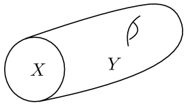
Figure 1: The Dai-Freed construction computes the phase of the fermion path integral on a manifold $X$ via an auxiliary manifold $Y$ such that $\partial Y=X$.

Then, out of the Dirac operator on $X$ showing up in the fermion lagrangian (2), we construct a Dirac operator in $Y$ by the prescription that near the boundary $X\times(-\tau_{0},0]$ of $Y$, $i\not{D}_{Y}$ takes the form

$$i\not{D}_{Y} =i\gamma^{\tau}\left(\frac{\partial}{\partial\tau}+i\not{D}_{X}^{\prime}\right),\quad\gamma^{\tau}=\text{diag}\,(\mathbf{I}_{d},-\mathbf{I}_{d}),$$

$$i\not{D}_{X}^{\prime}=\left(\begin{array}[]{cc}0&i\not{D}_{X}\\ -i\not{D}^{\dagger}_{X}&0\end{array}\right).$$ (14)

As mentioned before, there is an anomaly whenever the partition function (4) is not a well-defined function of the connection/metric. We can rephrase this by saying that the partition function is in general not a function on the space $\mathcal{M}$ of connections/metrics modulo gauge transformations/diffeomorphisms, but rather, a section of a nontrivial complex line bundle over $\mathcal{M}$, the so-called determinant line bundle over $\mathcal{M}$ Dai:1994kq (or Pfaffian line bundle in the general case).

The Dai-Freed theorem tells us that there is a quantity, computed solely in terms of $\not{D}_{Y}$,

$$\exp\left(2\pi i\eta_{Y}\right)$$ (15)

that is also a section of the same principal $U(1)$ bundle. As a result, we can use (15) instead of working with the determinant (5) directly to study anomalies. $\eta_{Y}$ is the Atiyah-Patodi-Singer (APS) $\eta$-invariant Atiyah:1975jf ; Atiyah:1976jg ; APS-III ; Witten:1985xe ; Witten:2015aba , defined as follows. First, we pick a class of boundary conditions (called APS boundary conditions Atiyah:1975jf ; Atiyah:1976jg ; APS-III , see Yonekura:2016wuc for a nice detailed discussion) such that $i\not{D}_{Y}$ on $Y$ becomes self-adjoint. Then, $\eta_{Y}$ is a regularized sum of eigenvalues

$$\eta_{Y}=\frac{1}{2}\left(\sum_{\lambda\neq 0}\text{sign}(\lambda)+\dim\ker(i\mathcal{D}_{Y})\right)_{\text{reg.}}.$$ (16)

The sum is infinite and requires regularization; $\zeta$-function regularization is commonly employed in the mathematical literature. The $\eta$ invariant jumps by $\pm 1$ whenever an eigenvalue crosses zero; however, $\exp(2\pi i\eta_{Y})$ is a continuous function of the gauge fields and the metric.

The advantages of this approach are that we now do not have to deal with regularizations, etc. directly, and that we can use several properties of the $\eta$ invariant to our advantage. For instance, $\eta$ behaves “nicely” under gluing Yonekura:2016wuc : if we have two manifolds $Y_{1},Y_{2}$ glued along a common boundary as in figure 2, giving the manifold $Y_{1}\sqcup Y_{2}$, we have

$$\exp(2\pi i\,\eta_{Y_{1}\sqcup Y_{2}})=\exp(2\pi i\,\eta_{Y_{1}})\exp(2\pi i\,\eta_{Y_{2}})\,.$$ (17)

This means that, as discussed in Monnier:2014txa for instance, if we want to compute the change of the phase of the partition function $Z[A]$, going from some configuration $A_{0}$ to some other $A_{0}^{g}$ (where $g$ may or may not be continuously connected to the identity) along a path $A_{t}$, we just need to compute the $\eta$ invariant on a manifold $X\times[0,1]$, since we can then glue it to the $Y_{0}$ which gives the phase on $A_{0}$ (see figure 3). Because the gauge configuration at the endpoints of the interval are gauge transformations of one another, we can glue the sides to obtain the $\eta$ invariant in the same mapping torus that was discussed above for global anomalies Yonekura:2016wuc .

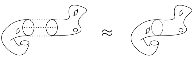
Figure 2: The $\eta$ invariant behaves nicely under gluing as illustrated in the picture.

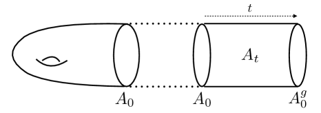
Figure 3: To obtain the phase for a configuration $A_{0}^{g}$ starting from $A_{0}$, we may just attach $X\times[0,1]$ as shown in the picture. The additional contribution to the phase is identical to $\eta$ evaluated on the mapping tours obtained by gluing the two sides of $X\times[0,1]$.

In this way, absence of traditional anomalies (local or global) becomes the requirement $\exp(2\pi i\,\eta_{Y})=1$ for $Y$ any mapping torus. We indeed recover the local and global anomaly cancellation conditions discussed above, as in Monnier:2014txa :

• For $g$ continuously connected to the identity, one can write $Y=\partial Z$, where $Z=X\times D$ is a $(d+2)$-dimensional manifold, since the gauge bundle can be extended to $Z$ without problem. In this case, we can use the APS index theorem for manifolds with boundary Atiyah:1975jf , which relates

  $$\text{Ind}(\not{D}_{Z})=\eta_{Y}+\int_{Z}\hat{A}(R)\operatorname{ch}(F).$$ (18)

  The left hand side is the index of a Dirac operator on $Z$, which is always an integer. Exponentiating, we get

  $$\exp(2\pi i\,\eta_{Y})=\exp\left(2\pi i\int_{Z}\hat{A}(R)\operatorname{ch}(F)\right)=\exp\left(2\pi i\int_{Z}I_{d+2}\right)\,.$$ (19)

  The only way the anomaly vanishes is if the anomaly polynomial vanishes identically. We thus recover the traditional local anomaly cancellation condition.

• Global anomalies of complex fermions were already discussed in terms of the $\eta$ invariant. This covers almost all the cases we will discuss in this paper. We refer the reader to Witten:2015aba for a discussion of the (pseudo-)real case.

In the present formalism, a natural question is whether the requirement $\exp(2\pi i\,\eta_{Y})=1$ should be generalized to closed $(d+1)$ manifolds $Y$ which are not mapping tori. These conditions do not correspond to anomalies in the traditional sense; yet demanding their vanishing can impose nontrivial constraints on the allowed theories. We will call them, for lack of a better term, “Dai-Freed anomalies” (even though also the traditional anomalies can also be nicely understood from the Dai-Freed point of view, as we have just seen). The goal of this paper is the exploration of these constraints in some interesting gauge theories. But before we start computing $\eta$ invariants, let us review some of the reasons why it seems plausible to us that these anomalies should cancel.

Suppose as before that we want to study the theory on some $X=\partial Y_{1}=\partial Y_{2}$. Then, we can glue $Y_{1}$ and $Y_{2}$ with opposite orientation along their common boundary, and we can compute $\exp(2\pi i\,\eta_{Y_{1}\sqcup\bar{Y}_{2}})$. If this is different from one, it means that the Dai-Freed prescription does not give a unique answer for the phase of the path integral. Faced with this issue we could somehow try to restrict the allowed set of $Y$’s to be used in the Dai-Freed prescription, so that e.g. $Y_{1}$ is allowed but $Y_{2}$ is not. However, this cannot be done arbitrarily; it has to be done in a consistent way with cutting and pasting relations Witten:2015aba . Reflection positivity/unitarity also provide further constraints. It seems more economical to impose $\exp(2\pi i\eta_{Y})=1$ for all closed $Y$ instead.

In systems coupled to dynamical gravity, there is another way to motivate imposing these constraints. Recall that a mapping torus for a global anomaly is just describing a non-contractible loop in the gauge field/metric configuration space. We get one mapping torus for each non-contractible loop. In quantum gravity, however, we generically expect topology change (there are a myriad examples of such behaviour understood by now in string theory, see e.g. Giddings:1987cg ; Witten:1998zw for two examples which are particularly close to what we are discussing here). Morally, this enlarges the configuration space, and one can now consider closed paths along which the topology changes. These will look like a “mapping torus with holes” such as the one in figure 4, and some of them might be non-contractible. From this point of view, the Dai-Freed anomalies are not different from the traditional ones, at least in a theory in which topology change is allowed.

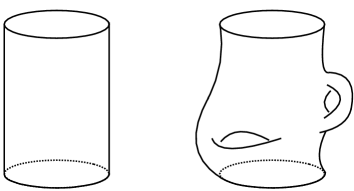
Figure 4: Traditional global anomalies are studied via the $\eta$ invariant on mapping tori (left figure). The general Dai-Freed anomaly can be regarded as a generalization in which we allow the “mapping torus” to have holes or other nontrivial topologies. In the same way that the traditional mapping torus follows a nontrivial loop in configuration space, the new anomaly can be regarded as coming from new nontrivial loops that arise once topology change is allowed, as one might expect to happen in quantum gravity.

While it is not obvious that any manifold $Y$ can be regarded as a “generalized mapping torus” as in figure 4, there is always a perhaps different manifold $Y^{\prime}_{X}$ with $\eta(Y)=\eta(Y^{\prime}_{X})$ and which has a mapping torus interpretation over a base manifold $X$ (so that it describes an anomaly for the theory on $X$). One can construct $Y^{\prime}_{X}$ by starting with a trivial mapping torus $X\times S^{1}$, for which the anomaly theory is trivial since it is a boundary, and then taking $Y^{\prime}_{X}$ to be the connected sum $(X\times S^{1})\#Y$. To display $Y_{X}^{\prime}$ as a generalized mapping torus, cut it open along the $S_{1}$, and embed the resulting $(X\times[0,1])\#Y$ into $\mathbb{R}^{K}$ (such an embedding is always possible for high enough $K$, as proven by Whitney). Slicing with hyperplanes parallel to the $[0,1]$ factor, one recovers the picture in figure 4.

For completeness, let us mention that the rephrasing of the anomaly for fermions in $X$ in terms of $\exp(2\pi i\,\eta_{Y})$ is a specific example of a more general construction, where one associates a $(d+1)$-dimensional anomaly theory $\mathcal{A}[\mathcal{T}]$ to any anomalous $d$-dimensional theory $\mathcal{T}$, such that the anomalous behaviour of the partition function of $\mathcal{T}$ on some manifold $X_{d}$ is encoded (in the same manner as above) in the behavior of $\mathcal{A}[\mathcal{T}]$ on $Y_{d+1}$, with $X_{d}=\partial Y_{d+1}$. In our case we have $d=4$, $\mathcal{T}$ is the theory of a Weyl fermion charged under some global symmetry $G$, and $\mathcal{A}[\mathcal{T}]$ is $\exp(2\pi i\,\eta_{Y})$. Other important cases for which one can proceed analogously, and construct appropriate anomaly theories, are theories with self-dual fields in $d=4k+2$ dimensions, theories with Rarita-Schwinger fields, and theories where the Green-Schwarz anomaly cancellation mechanism operates. We refer the reader to Freed:2014iua ; Monnier:2019ytc for a systematic discussion of such generalizations, and further references to the literature.

Finally, it should be pointed out that there is the possibility of anomaly cancellation mechanisms which in some cases might weaken the requirement of having $\exp(2\pi i\,\eta_{Y})=1$ for every $Y$. The ordinary Green-Schwarz mechanism is one example, where the anomaly can sometimes be cancelled by adding suitable non-invariant terms to the Lagrangian. Relatedly, as discussed in Garcia-Etxebarria:2017crf , anomalies which only appear for spacetimes with specific topological properties may sometimes be cancelled by coupling to a topological QFT with the same anomaly. When such a possibility exists, it is perfectly fine to have a Dai-Freed anomalous sector, as long as we “cure” the anomaly by coupling to the right TQFT. This means that any claim we make below of a theory having a Dai-Freed anomaly should be understood to mean that the theory is inconsistent if not coupled to any TQFT, and may in some cases become consistent by such a coupling, but the criterion for which cases are fixable is currently unknown. We will present explicit examples in section 4.6 where such a possibility plays a very important role in connecting with known results. See Benini:2018reh for more examples of TQFTs with the same anomaly as local quantum field theories of interest, also applying to generalized global symmetries.

Luckily, the claim of consistency is not subject to such uncertainties: for the cases for which we prove absence of Dai-Freed anomalies one can state with certainty that anomalies are absent. It is still interesting to couple the theory to non-trivial TQFTs, and perhaps some of these introduce anomalies, but it is not something one needs to do.

2.2 Mathematical tools

The rest of the paper is devoted to analyzing Dai-Freed anomalies in theories of interest. To do this, we need a number of mathematical tools that we review in this section.

2.2.1 The general strategy: $\eta$ and bordism

In the rest of the paper, we will only consider theories in which the local anomalies cancel. This has the very convenient consequence that $\eta$ becomes a topological invariant, and in fact it has the stronger property of being a bordism invariant.

Bordism is an equivalence relation between manifolds (possibly equipped with extra structure): $Y_{1}$ and $Y_{2}$ are bordant if their disjoint union with a change of orientation for $Y_{2}$, which we denote as $Y_{1}\sqcup\bar{Y}_{2}$, is the boundary of another manifold $Z$, as illustrated in figure 5. If this is the case, we write $Y_{1}\sim Y_{2}$, which is clearly an equivalence relation. In case the $Y_{i}$ carry extra structure, such as a spin structure or a gauge bundle, we demand that this can be extended to $Z$ as well.

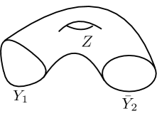
Figure 5: The two manifolds $Y_{1}$ and $Y_{2}$ are bordant if $Y_{1}\sqcup\bar{Y_{2}}$ is boundary of another manifold $Z$.

Bordism invariance of $\exp(2\pi i\,\eta_{Y})$ is a simple consequence of the APS index theorem (18) and the fact that local anomalies cancel, so the last term in (18) is absent. To see this, we use the fact that under change of orientation

$$\exp(2\pi i\,\eta_{\overline{Y}})=\exp(-2\pi i\,\eta_{Y})$$ (20)

so that the gluing properties of $\eta$ imply

$$\exp(2\pi i\,\eta_{Y_{1}\sqcup\overline{Y_{2}}})=\frac{\exp(2\pi i\,\eta_{Y_{1}})}{\exp(2\pi i\,\eta_{Y_{2}})}\,.$$ (21)

If $Y_{1}$ and $Y_{2}$ are in the same bordism class then, by definition, $Y_{1}\sqcup\overline{Y_{2}}$ is a boundary of some manifold $Z$, so by (19) we have

$$\frac{\exp(2\pi i\,\eta_{Y_{1}})}{\exp(2\pi i\,\eta_{Y_{2}})}=\exp(2\pi i\,\eta_{Y_{1}\sqcup\overline{Y_{2}}})=\exp(2\pi i\int_{Z}I_{d+2})=1$$ (22)

assuming no local anomalies.

Furthermore, the set of bordism equivalence classes forms an abelian group under union; we define $[Y_{1}]+[Y_{2}]=[Y_{1}\sqcup Y_{2}]$. This also works when additional structures are present.

We will be particularly interested in the bordism groups denoted $\Omega_{d}^{\mathrm{Spin}}(W)$, whose elements are equivalence classes of $d$-dimensional Spin manifolds equipped with a map to $W$. To study gauge anomalies in a theory with a symmetry group $G$, we will take $W=BG$, the classifying space of $G$. This is an infinite-dimensional space equipped with a principal $G$-bundle with total space $EG$, with the universal property that any principal $G$-bundle over any manifold $X$ is the pullback $f^{*}EG$ via some map $f:X\rightarrow BG$. Thus, the set of all topologically distinct principal bundles over any given manifold $X$ is equivalent to the set $[X,BG]$ of homotopy classes of maps from $X$ to $BG$. The classifying space is therefore a convenient way to describe principal bundles. See Guo:2017xex ; Wang:2018edf for a similar discussion in the context of $3+1$ topological insulators, where similar bordism groups (and twisted generalizations thereof) are computed.

In a $d$-dimensional theory with spinors and symmetry group $G$, the Dai-Freed anomaly $\exp(2\pi i\,\eta_{Y})$ is a group homomorphism from $\Omega_{d+1}^{\mathrm{Spin}}(BG)$ to $U(1)$. To study these anomalies we will follow these two steps:

• Compute $\Omega_{d+1}^{\mathrm{Spin}}(BG)$. If it vanishes, there can be no Dai-Freed anomaly.

• If $\Omega_{d+1}^{\mathrm{Spin}}(BG)\neq 0$, compute $\exp(2\pi i\,\eta)\colon\Omega_{d+1}^{\mathrm{Spin}}(BG)\rightarrow U(1)$, typically by explicit computation on convenient generators of the bordism group.

For the theories of interest in this paper, the first step can be performed fairly systematically via spectral sequences, which we will introduce in the next subsection. The second step is more artisanal — we need to analyze and compute $\eta$ in a case-by-case basis. We will give examples in section 4.

2.2.2 The Atiyah-Hirzebruch spectral sequence

A nice introduction to spectral sequences is McCleary , we will just cover the essentials to understand how the computation works. The Atiyah-Hirzebruch spectral sequence (AHSS) is a tool for computing the generalized homology groups $E_{*}(X)$ of some space $X$. A generalized homology theory satisfies the same axioms as ordinary homology, except for the dimension axiom: $H_{p}(\mathrm{pt})$ — the homology groups of a point — do not necessarily vanish for $p\neq 0$. It turns out that bordism theories $\Omega^{\mathrm{Spin}}_{*}(X)$ (and similarly $\Omega_{*}^{\mathrm{Pin}^{\pm}}(X)$) are generalized homology theories on $X$.

The AHSS works as follows. Suppose we have a Serre fibration $F\rightarrow X\rightarrow B$. Then the AHSS provides a systematic way to obtain a filtration of $\Omega^{\mathrm{Spin}}_{n}(X)$, that is a sequence of spaces

$$0=F_{-1}\Omega^{\mathrm{Spin}}_{n}(X)\subset F_{0}\Omega^{\mathrm{Spin}}_{n}(X)\subset\ldots\subset F_{n}\Omega^{\mathrm{Spin}}_{n}(X)=\Omega^{\mathrm{Spin}}_{n}(X)\,.$$ (23)

Specifically, the AHSS provides a way to compute the quotients

$$E_{k,n-k}^{\infty}=\frac{F_{k}\Omega^{\mathrm{Spin}}_{n}(X)}{F_{k-1}\Omega^{\mathrm{Spin}}_{n}(X)}\,.$$ (24)

Even when all these quotients are known, they do not fully determine $\Omega^{\mathrm{Spin}}_{*}(X)$. One has to solve the successive extension problems associated to (23) and (24), which may require additional information.

The quotients $E^{\infty}_{p,q}$ live on the “$\infty$ page” of the spectral sequence, and they are computed as follows. The “second page” of the AHSS is simply

$$E^{2}_{p,q}=H_{p}(B,\Omega_{q}^{\mathrm{Spin}}(F))\,.$$ (25)

The $r$-th page comes equipped with a differential $d_{r}\colon E_{p,q}^{r}\rightarrow E_{p-r,q+r-1}$, with $d_{r}^{2}=0$. The next page in the spectral sequence, $E^{r+1}$, is the cohomology of $E^{r}$ under $d_{r}$.

A spectral sequence is usually presented in a diagram such as that of figure 6. The differentials are represented by arrows. For a given entry in the spectral sequence, there are no more differentials that can act on it after a finite number of pages; we then say that the sequence stabilizes (for the entry of interest) and we can read off $E^{\infty}_{p,q}$.

Figure 6: Generic structure of a spectral sequence. The sequence consists of “pages” (in the figure we depict the second and third pages), and to turn to the next page one needs to take the cohomology with respect to the differential $d_{r}$. The differentials at each page are represented by arrows. Some entries might be “killed” by the differentials. After we are done, at $E^{\infty}$, $\Omega^{\mathrm{Spin}}_{n}(E)$ is obtained by solving an extension problem involving all the entries with $p+q=n$.

The generic strategy we will use to compute $\Omega_{*}^{\mathrm{Spin}}(BG)$ is the AHSS associated to the fibration $\mathrm{pt}\rightarrow BG\rightarrow BG$, which relates $\Omega_{*}^{\mathrm{Spin}}(BG)$ to the groups $\Omega_{q}^{\mathrm{Spin}}(\mathrm{pt})$, which are given by ABP ; Stong-11 ; Kapustin:2014dxa

$$\begin{array}[]{c|ccccccccccc}n&0&1&2&3&4&5&6&7&8&9&10\\ \hline\cr\Omega^{\mathrm{Spin}}_{n}(\mathrm{pt})&\mathbb{Z}&\mathbb{Z}_{2}&\mathbb{Z}_{2}&0&\mathbb{Z}&0&0&0&2\mathbb{Z}&2\mathbb{Z}_{2}&3\mathbb{Z}_{2}\end{array}$$ (26)

where with the notation $k\mathbb{Z}$ we mean simply $\mathbb{Z}\oplus\ldots\oplus\mathbb{Z}$, $k$ times.

2.2.3 Evaluating the first nontrivial differentials: Steenrod squares & their duals

In the applications that will be discussed in section 3, it will often be the case that the differentials in the AHSS cannot be determined by algebraic considerations alone. In some cases, however, we will be able to determine $d_{2}$ via Lemma 2.3.2 of TeichnerPhD (also the Lemma in pg. 751 of Teichner ), which says that for $X$ a spectrum, the differential $E_{2}^{(p,0)}\to E_{2}^{(p-2,1)}$, that is

$$d_{2}\colon H_{p}(X,\Omega_{0}^{\mathrm{Spin}})\rightarrow H_{p-2}(X,\Omega_{1}^{\mathrm{Spin}})\,,$$ (27)

is the composition of reduction mod 2 $\rho$ with the dual $\mathrm{Sq}_{*}^{2}$ (with respect to the Kronecker pairing between homology and cohomology adams1995stable ) of the second Stenrood square $\mathrm{Sq}^{2}$. That is, $\bigl{\langle}a,\mathrm{Sq}^{2}b\bigr{\rangle}=\bigl{\langle}\mathrm{Sq}_{*}^{2}a,b\bigr{\rangle}$ for any $a,b$, where $\bigl{\langle},\bigr{\rangle}$ is the Kronecker pairing between $H_{n}(X,\mathbb{Z}_{2})$ and $H^{n}(X,\mathbb{Z}_{2})$, which is simply the evaluation map.

Note the fact that $H^{n}(X,\mathbb{Z}_{2})=H_{n}(X,\mathbb{Z}_{2})$. This follows from the universal coefficient theorem with coefficients in an arbitrary ring (Theorem 3.2 of Hatcher:478079 )

$$0\to\operatorname{Ext}_{R}^{1}(H_{i-1}(X,R),G)\to H^{i}(X,G)\to\operatorname{Hom}_{R}(H_{i}(X,R),G)\to 0$$ (28)

and $\operatorname{Ext}_{\mathbb{Z}_{2}}^{1}(H_{i-1}(X,\mathbb{Z}_{2}),\mathbb{Z}_{2})=0$ since $\mathbb{Z}_{2}$ is injective as a module over itself. We thus have that $H^{i}(X,\mathbb{Z}_{2})\cong\operatorname{Hom}_{\mathbb{Z}_{2}}(H_{i}(X,\mathbb{Z}_{2}),\mathbb{Z}_{2})$, with the isomorphism induced by the Kronecker pairing above.

Similarly,

$$d_{2}:H_{p}(X,\Omega_{1}^{\mathrm{Spin}})\rightarrow H_{p-2}(X,\Omega_{2}^{\mathrm{Spin}})$$ (29)

is simply the dual Steenrod square.

Steenrod squares $\mathrm{Sq}^{i}$ are certain cohomology operations which we can compute explicitly in the examples of interest, using the following properties. (Here $u_{i}\in H^{i}(X,\mathbb{Z}_{2})$.)

$$\mathrm{Sq}^{0}u_{i} =u_{i}\,,$$ (30a)

$$\mathrm{Sq}^{i}u_{i} =u_{i}^{2}\,,$$ (30b)

$$\mathrm{Sq}^{j}u_{i} =0\qquad\text{for }j>i\ ,$$ (30c)

$$\mathrm{Sq}^{n}(a\smile b) =\sum_{i+j=n}(\mathrm{Sq}^{i}a)\smile(\mathrm{Sq}^{j}b)\,.$$ (30d)

The last equation is known as Cartan’s formula. We refer interested readers to WuSteenrod ; Borel1953 ; milnor1974characteristic ; Fung ; Hatcher:478079 for further details.

Reduction modulo 2 above refers to the map $\rho$ in the exact sequence

$$\ldots\to H_{i}(X,\mathbb{Z})\to H_{i}(X,\mathbb{Z})\xrightarrow{\,\rho\,}H_{i}(X,\mathbb{Z}_{2})\to H_{i-1}(X,\mathbb{Z})\ldots$$ (31)

associated to the short exact sequence $0\to\mathbb{Z}\to\mathbb{Z}\to\mathbb{Z}_{2}\to 0$.

Finally, the homology groups of a spectrum $\{X_{n},s_{n}\}$ are defined as

$$H_{k}(X)=\text{colim}_{n}H_{k+n}(X_{n})$$ (32)

If $X$ is the suspension spectrum of $X_{0}$, defined by $X_{n}=\Sigma^{n}X_{0}$ and $s_{n}$ the identity, we can use the result Hatcher:478079

$$H_{k+n}(\Sigma^{n}X_{0})=H_{k}(X_{0})$$ (33)

to obtain that (27) and (29) also apply to an ordinary CW complex, such as the classifying spaces we will be interested in.

We are now in position to follow the strategy outlined in section 2.2.1 in a number of interesting cases, which we discuss in the following sections.

3 Dai-Freed anomalies of some simple Lie groups

3.1 $SU(2)$

As a warm-up, we will start with $SU(2)$. To get the AHSS to work, we need the homology of its classifying space $BSU(2)$. This is known to be $BSU(2)=\mathbb{H}\mathbb{P}^{\infty}$, the infinite-dimensional quaternionic projective space (see e.g. Marathe:2010ncz , section 5.2), obtained as the limit of the natural inclusions $\mathbb{H}\mathbb{P}^{n}\to\mathbb{H}\mathbb{P}^{n+1}$. The homology groups of this space are very simple to obtain, we have

$$H_{n}(\mathbb{H}\mathbb{P}^{\infty},\mathbb{Z})=\begin{cases}\mathbb{Z}\quad&\text{when }n\equiv 0\text{ mod }4\,,\\ 0\quad&\text{otherwise}\,.\end{cases}$$ (34)

We also need a way of computing $H_{p}(\mathbb{H}\mathbb{P}^{\infty},\Omega_{q}^{\mathrm{Spin}})$ out of knowledge of $H_{n}(\mathbb{H}\mathbb{P}^{\infty},\mathbb{Z})$ and $\Omega_{q}^{\mathrm{Spin}}$. This is a task for the universal coefficient theorem, which in its homological version implies (see theorem 3A.3 in Hatcher:478079 ) that there is a short exact sequence

$$0\to H_{n}(\mathbb{H}\mathbb{R}^{\infty},\mathbb{Z})\otimes\Omega^{\mathrm{Spin}}_{q}\to H_{n}(\mathbb{H}\mathbb{P}^{\infty},\Omega^{\mathrm{Spin}}_{q})\to\operatorname{Tor}(H_{n-1}(\mathbb{H}\mathbb{P}^{\infty},\mathbb{Z}),\Omega_{q}^{\mathrm{Spin}})\to 0\,.$$ (35)

Since $H_{n}(\mathbb{H}\mathbb{P}^{\infty},\mathbb{Z})$ is free, we have that $\operatorname{Tor}(H_{n-1}(\mathbb{H}\mathbb{P}^{\infty},\mathbb{Z}),\Omega_{q}^{\mathrm{Spin}}))=0$, and thus

$$H_{n}(\mathbb{H}\mathbb{P}^{\infty},\Omega^{\mathrm{Spin}}_{q})\cong H_{n}(\mathbb{H}\mathbb{R}^{\infty},\mathbb{Z})\otimes\Omega^{\mathrm{Spin}}_{q}=\begin{cases}\Omega^{\mathrm{Spin}}_{q}\quad&\text{when }n\equiv 0\text{ mod }4\,,\\ 0\quad&\text{otherwise}\,.\end{cases}$$ (36)

Figure 7: $E_{4}$ page of the AHSS for $\Omega^{\mathrm{Spin}}_{*}(BSU(2))$. We have shaded the entries of total degree 5, and indicated explicitly the only potentially non-vanishing differential acting on the shaded region.

We have now the necessary information for constructing the AHSS. It is clear from the fact that the differential $d_{r}$ has bi-degree $(-r,r-1)$, that $E_{4}=E_{3}=E_{2}$. More generally, it is only differentials of the form $d_{4k}$ that can vanish.

We show this fourth page in figure 7. There is a priori a nonvanishing differential $d_{4}\colon\mathbb{Z}_{2}\to\mathbb{Z}$, but since it is a homomorphism we necessarily have $d_{4}=0$. This shows that $E_{4,1}^{\infty}=E_{4,1}^{2}=\mathbb{Z}_{2}$. Since all the other elements with total degree 5 vanish already in $E_{2}$, we conclude that

$$\Omega_{5}^{\mathrm{Spin}}(BSU(2))=\mathbb{Z}_{2}\,.$$ (37)

A bordism invariant that we can construct in this case, since $SU(2)$ has no local anomalies, is the $\eta$ invariant, or equivalently (in this case) the mod-2 index. A simple example with non-vanishing mod-2 index was constructed in Witten:1982fp . While $S^{5}$ itself is trivial in $\Omega^{\mathrm{Spin}}_{5}$ (necessarily so, since $\Omega^{\mathrm{Spin}}_{5}=0$), there is a bundle over it such that the total space is no longer null-bordant in $\Omega^{\mathrm{Spin}}_{5}(BSU(2))=\mathbb{Z}_{2}$. What (37) shows is that the four dimensional theory of a Weyl fermion on the fundamental of $SU(2)$ has no further gauge anomalies on any $\mathrm{Spin}$ manifold (the calculation in Witten:1982fp shows absence of anomalies in $S^{4}$). This was to be expected: since a Weyl fermion in the fundamental of $SU(2)$ is in a real representation of the full (Lorentz plus gauge) symmetry group, it has at most a $\mathbb{Z}_{2}$ anomaly.

It is trivial to repeat the argument for other (low enough) dimensions, we find

$$\begin{array}[]{c|ccccccccc}n&0&1&2&3&4&5&6&7&8\\ \hline\cr\Omega^{\mathrm{Spin}}_{n}(BSU(2))&\mathbb{Z}&\mathbb{Z}_{2}&\mathbb{Z}_{2}&0&2\mathbb{Z}&\mathbb{Z}_{2}&\mathbb{Z}_{2}&0&4\mathbb{Z}\end{array}$$ (39)

The only non-trivial case here is that of $\Omega_{4}^{\mathrm{Spin}}(BSU(2))$ (and $\Omega_{8}^{\mathrm{Spin}}(BSU(2))$, which works similarly). This has two contributions, coming from $E_{4,0}^{\infty}=\mathbb{Z}$ and $E_{0,4}^{\infty}=\mathbb{Z}$.

One point that we have neglected so far is that the spectral sequence does not give us $\Omega^{\mathrm{Spin}}_{k}(BSU(2))$ directly, but rather an associated graded module $\textsf{Gr}_{p,q}$ McCleary , which depends, as discussed in Subsection 2.2.2 in addition to the bordism group itself, on a suitable filtration by graded submodules $F_{p}$. Spectral sequences compute $\textsf{Gr}_{p,q}=E^{\infty}_{p,q}$. Tracing the definitions, we find that

$$F_{3}\Omega_{4}=F_{2}\Omega_{4}=F_{1}\Omega_{4}=F_{0}\Omega_{4}=\textsf{Gr}_{0,4}=E^{\infty}_{0,4}=\mathbb{Z}\,.$$ (40)

On the other hand, we have $E^{\infty}_{4,0}=\textsf{Gr}_{4,0}=F_{4}\Omega_{4}/F_{3}\Omega_{4}$. We are interested in solving for $\Omega_{4}=F_{4}\Omega_{4}$. We can do this, formally, by fitting the above into a short exact sequence

$$0\to\underbrace{F_{3}\Omega_{4}}_{\mathbb{Z}}\to F_{4}\Omega_{4}\to\underbrace{\textsf{Gr}_{4,0}}_{\mathbb{Z}}\to 0\,.$$ (41)

Since $\operatorname{Ext}(\mathbb{Z},\mathbb{Z})=0$ Hatcher:478079 , the exact sequence necessarily splits, and we have $\Omega_{4}=F_{4}\Omega_{4}=\mathbb{Z}\oplus\mathbb{Z}$.

3.1.1 Physical interpretation

Obstructions to a manifold being trivial in its Spin bordism class can be detected by computation of certain suitable KO-theory classes ABP . This is a fancy way of saying that there is some (perhaps mod-2) index that can detect the non-triviality of the manifold. For instance, on an $S^{1}$, with the periodic structure, the mod-2 index is non-vanishing, and similarly for the $T^{2}$ with completely periodic structure (see pg. 45 of Witten:2015aba ). In these low dimensions there is no topologically nontrivial $SU(2)$ bundle, so what we are seeing is the fact that $\Omega_{1}^{\mathrm{Spin}}(BSU(2))=\Omega_{1}^{\mathrm{Spin}}(\mathrm{pt})$. (More formally, this comes from the fact that every $p$-cycle is contractible in $BSU(2)=\mathbb{H}\mathbb{P}^{\infty}$ for $p<4$.)

The $\mathbb{Z}_{2}$ values in 5 and 6 dimensions encode global anomalies in $SU(2)$ theories in 4d with a Weyl fermion and 5d with a symplectic Majorana fermion Intriligator:1997pq .

In four dimensions we get an extra factor of $\mathbb{Z}$ with respect to $\Omega_{4}^{\mathrm{Spin}}(\mathrm{pt})$. This anomaly can be associated to the global parity anomaly of Redlich Redlich:1983kn ; Redlich:1983dv , for a Dirac fermion in the fundamental of $SU(2)$. To see this, we need need to construct the right bordism invariants that detect both $\mathbb{Z}$ factors. We know that the invariant that detects the class in $\Omega^{\mathrm{Spin}}_{4}(\mathrm{pt})$ is simply the Pontryagin number. The class detecting the extra information in $\Omega^{\mathrm{Spin}}_{4}(BSU(2))$ is the index of a Weyl fermion on the manifold, which is indeed related to the parity anomaly in 3d.

The 8d case is related to parity anomalies in 7d. The relevant Chern-Simons terms are those associated with $p_{1}(T)^{2}$, $p_{2}(T)$, $p_{1}(F)^{2}$ and $p_{1}(T)p_{1}(F)$, with $p_{i}$ the Pontryagin classes of the tangent bundle $T$ and the gauge bundle $F$.

3.1.2 Simply connected semi-simple groups up to five dimensions

The structure we have just discussed for $SU(2)$ is actually very general in low enough dimension and applies to the simply connected forms of all semisimple Lie groups, as we now explain. First, notice that, for any such $G$, $\pi_{1}(G)=\pi_{2}(G)=0$, $\pi_{3}(G)=\mathbb{Z}$. We can now use the result that (see §8.6.4 of husemoller )

$$\pi_{i+1}(BG)=\pi_{i}(G)$$ (42)

for any group $G$ and $i\geq 0$, to compute that

$$\pi_{i}(BG)=\{0,0,0,0,\mathbb{Z},\pi_{4}(G),\ldots\}$$ (43)

Note in particular that $BG$ is 3-connected. Applying the Hurewicz theorem Hatcher:478079 we find that

$$H_{i}(BSU(n),\mathbb{Z})=\{\mathbb{Z},0,0,0,\mathbb{Z},s(\pi_{4}(G)),\ldots\}\,.$$ (44)

where $s(\pi_{4}(G))$ denotes some subgroup of $\pi_{4}(G)$ to be determined. A couple of points require explanation. First, note that the Hurewicz isomorphism only holds for $i>0$. We used the input (43) to set $H_{i}(BG,\mathbb{Z})=\mathbb{Z}$, in contrast to $\pi_{0}(BG)=0$. The standard statement for the Hurewicz isomorphism in our case is that $\pi_{i}(BG)=H_{i}(BG,\mathbb{Z})$ up to $i=4$, see for example theorem 4.37 in Hatcher:478079 . To set $H_{5}(BG,\mathbb{Z})$ we have used that the Hurewicz homomorphism is surjective for $i=5$ in a 3-connected space, see exercise 23 in §4.2 of Hatcher:478079 . Whenever $\pi_{4}(G)=0$, as is the case for $SU(n)$, $Spin(n)$, and the exceptional groups, we have that $H_{5}(BG,\mathbb{Z})=0$.

The information in (44) is enough to compute $\Omega_{k}^{\mathrm{Spin}}(BG)$ up to $k=4$ via the AHSS, with results identical to the $SU(2)$ case. For the case $\pi_{4}(G)=0$, we also find that the bordism group $\Omega_{5}^{\mathrm{Spin}}(BG)$ is given by

$$\Omega_{5}^{\mathrm{Spin}}(BG)=\operatorname{coker}(d_{2}\colon E^{(6,0)}_{2}\to E_{2}^{(4,1)})\,.$$ (45)

Luckily, this is a differential for which we have an explicit expression, as reviewed in section 2.2.3. Part of the rest of this section will be about the explicit computation of this differential in various interesting examples.

Finally, we should remark that the construction of the AHSS (see e.g. Diaconescu:2000wy ) also provides a natural candidate for the representative of $E_{2}^{(4,1)}=H_{4}(BG,\Omega_{1}^{\mathrm{Spin}})$. We need a manifold with a $S^{1}$ with a spin structure that does not bound, and with a $G$-bundle with nontrivial second Chern class, since this is measured by $H_{4}(BG)$. The natural candidate is $S^{4}\times S^{1}$, with periodic boundary conditions along the $S^{1}$, and a gauge instanton on $S^{4}$. The question is whether or not this is trivial in spin bordism, which we now address in a number of examples.

If all one is interested in is the anomaly on four dimensional $\mathrm{Spin}$ manifolds there is a shortcut based on the previous observation: one can detect the anomaly in the original four dimensional theory by reducing along an $S^{4}$ with an instanton bundle, and seeing whether the effective zero-dimensional theory is anomalous, as done for instance in Garcia-Etxebarria:2017crf .

A second shortcut exists for simply connected groups in five dimensions: say that we have a group $G$ with subgroup $H$, and we want to understand whether we can deform any $G$ bundle over a base $X$ to a $H$ bundle over $X$. If we can, and assuming that the $G$ theory is free of local anomalies, then we can compute the $\eta$ invariant from knowledge of the $\eta$ invariant of the $H$ theory. As reviewed in Witten:1985bt ; Diaconescu:2000wy , for instance, the reduction is in fact possible if $\pi_{i}(G/H)=0$ for all $i<\dim(X)$. Take $H=SU(2)$, where we have already understood what happens. One has $SU(n+1)/SU(n)=S^{2n+1}$, and in particular $SU(3)/SU(2)=S^{5}$. This implies that in five dimensions any $SU(3)$ bundle can be reduced to an $SU(2)$ bundle, since $\pi_{i}(S^{5})=0$ for $i<5$. Similarly, by studying higher values of $n$, one can show that every $SU(n)$ bundle can be reduced to an $SU(2)$ bundle. It is not difficult to extend this result to the other simply connected Lie groups, which effectively reduces the problem of computing anomalies in these cases to a group theory analysis.

While these techniques (and related ones) often lead to an economic derivation in specific cases, we have opted to proceed by computing of the bordism groups using the Atiyah-Hirzebruch spectral sequence, since it is a viewpoint that straightforwardly applies to other situations of interest that do not admit the shortcuts above.

3.2 $U\!Sp(2k)$

The $U\!Sp(2k)$ case is very similar to $U\!Sp(2)=SU(2)$, so we will be brief. The classifying space $BU\!Sp(2k)$ is given by the infinite quaternionic Grassmanian, we refer the reader to FuchsViro for details of the homology of this space. The relevant AHSS is shown in figure 8, where we have shown specifically the $U\!Sp(2k)$ case with $k>1$.

Figure 8: $E_{8}$ page of the AHSS for $\Omega^{\mathrm{Spin}}_{*}(BU\!Sp(2k))$ with $k>1$. We have shaded the entries of total degree 9, and indicated explicitly the only potentially non-vanishing differential acting on the shaded region.

From figure 8, it is straightforward to see that $\Omega_{5}^{\mathrm{Spin}}(U\!Sp(2k))=\mathbb{Z}_{2}$, just like in the $SU(2)$ case. Indeed, this $\mathbb{Z}_{2}$ is related to a global anomaly in four dimensions, coming from the fact that $\pi_{4}(U\!Sp(2k))\neq 0$ as in the ordinary Witten anomaly. Just as in this case, the anomaly can be probed by a mod 2 index.

The first difference between $SU(2)$ and $U\!Sp(2k)$ with $k>1$ appears in eight dimensions, and it is due to the fact that while $SU(2)$ bundles are classified by $p_{1}^{2}(F)$, $U\!Sp(2k)$ bundles with $k>1$ are classified by two independent quantities: $p_{1}^{2}(F)$ and $p_{2}(F)$. More formally

$$H_{8}(BU\!Sp(2k),\mathbb{Z})=H^{8}(BU\!Sp(2k),\mathbb{Z})=\begin{cases}\mathbb{Z}&\quad\text{if }k=1\,,\\ \mathbb{Z}\oplus\mathbb{Z}&\quad\text{if }k>1\,.\end{cases}$$ (46)

This leads to a qualitative difference between the $k=1$ and $k>1$ cases when it comes to eight-dimensional anomalies. Consider for example a fermion in the adjoint representation. It was shown in Garcia-Etxebarria:2017crf that $k>1$ had an anomaly on spacetimes of non-trivial topology (the example analyzed there was that of spacetimes with a $S^{4}$ factor, and a unit of instanton flux on this factor, but the conclusion is clearly more general), while $k=1$ did not have this anomaly.

3.3 $U(1)$

Let us consider now the computation of $\Omega_{*}^{\mathrm{Spin}}(BU(1))$. This is the first case in which we will encounter non-vanishing differentials in the spectral sequence for the entries of interest. Recall that $BU(1)=K(Z,2)=\mathbb{C}\mathbb{P}^{\infty}$, so the relevant homology groups are well known:

$$H_{i}(BU(1),\mathbb{Z})=\begin{cases}\mathbb{Z}\quad\text{if }i\in 2\mathbb{Z}\,,\\ 0\quad\text{otherwise.}\end{cases}$$ (47)

From here, we obtain the AHSS shown in figure 9.

Figure 9: $E_{2}$ page of the AHSS for $\Omega^{\mathrm{Spin}}_{*}(BU(1))$. We have shaded the entries of total degree 5, and indicated explicitly the only potentially non-vanishing differential acting on the shaded region.

We see that there are two potentially non-vanishing differentials, both on the second page, $\alpha\colon E^{2}_{(6,0)}\to E^{2}_{(4,1)}$ and $\beta\colon E^{2}_{(4,1)}\to E^{2}_{(2,2)}$.

Let us start with $\alpha$. As reviewed in section 2.2.3, from TeichnerPhD ; Teichner we have that this differential is given by the composition of reduction modulo two and the dual of the Steenrod square

$$\mathrm{Sq}^{2}\colon H^{4}(BU(1),\mathbb{Z}_{2})\to H^{6}(BU(1),\mathbb{Z}_{2})\,.$$ (48)

Recall that $H^{i}(BU(1),\mathbb{Z})=\mathbb{Z}[x]$, with $x$ of degree two, so analogously (by the universal coefficient theorem in cohomology) $H^{i}(BU(1),\mathbb{Z}_{2})=\mathbb{Z}_{2}[x]$. Now, since $x$ is of degree 2, we have

$$\mathrm{Sq}^{2}(x)=x^{2}$$ (49)

and for degree reasons $\mathrm{Sq}^{1}(x)=0$. From here, using Cartan’s formula, we find that

$$\mathrm{Sq}^{2}(x^{2})=\mathrm{Sq}^{0}(x)\smile\mathrm{Sq}^{2}(x)+\mathrm{Sq}^{2}(x)\smile\mathrm{Sq}^{0}(x)=2x^{2}=0\,.$$ (50)

This implies that the dual Steenrod square also vanishes, and we conclude that

$$\alpha=\mathrm{Sq}_{*}^{2}\circ r_{2}=0\,.$$ (51)

We can deal with the $\beta$ differential similarly. According to TeichnerPhD ; Teichner we have $\beta=\mathrm{Sq}_{*}^{2}$. Using (49) we immediately see that $\mathrm{Sq}_{*}^{2}$ maps the generator of $H_{4}(BU(1),\mathbb{Z}_{2})$ to the generator of $H_{2}(BU(1),\mathbb{Z}_{2})$, so we immediately conclude that

$$\Omega_{5}^{\mathrm{Spin}}(BU(1))=0\,.$$ (52)

Similar arguments can be repeated for lower degrees, with the result

$$\begin{array}[]{c|cccccc}n&0&1&2&3&4&5\\ \hline\cr\Omega_{n}^{\mathrm{Spin}}(BU(1))&\mathbb{Z}&\mathbb{Z}_{2}&\mathbb{Z}_{2}\oplus\mathbb{Z}&0&\mathbb{Z}\oplus\mathbb{Z}&0\end{array}$$ (53)

The obvious interpretation of these results is that the $U(1)$ flux adds the natural obstruction, on top of that coming from $\Omega_{*}^{\mathrm{Spin}}(\mathrm{pt})$.

3.4 $SU(n)$ and implications for the Standard Model

Let us now compute $\Omega^{\mathrm{Spin}}_{*}(BSU(n))$. The classifying space of $SU(n)$ is well known to be the infinite Grassmanian of $n$-planes in $\mathbb{C}^{\infty}$. The integer cohomology ring of this space is very well known borel1955 ; Fung to be the polynomial ring

$$H^{*}(BSU(n),\mathbb{Z})=\mathbb{Z}[c_{2},c_{3}\ldots c_{n}].$$ (54)

The generators are the Chern classes; indeed, for a $SU(n)$-bundle over a space $X$ defined by a map $f\colon X\rightarrow BG$, the Chern classes of the bundle are the pullbacks $f^{*}(c_{i})$.

The universal coefficient theorem for cohomology Hatcher:478079 provides a short exact sequence relating the homology groups $H_{i}(X,\mathbb{Z})$ with the cohomology groups $H^{i}(X,\mathbb{Z})$:

(55)

If the homology groups are finitely generated, the $\operatorname{Ext}$ term is just the torsion part of $H_{i-1}(X,\mathbb{Z})$, and the Hom is the free part of $H_{i}(X,\mathbb{Z})$.

If $H^{i}(X,\mathbb{Z})=0$ for $i$ odd and there is no torsion in cohomology, such as for $BSU(n)$, we get $H_{i}(X,\mathbb{Z})=H^{i}(X,\mathbb{Z})$, with the resulting AHSS shown in figure 10.

Figure 10: $E_{2}$ page of the AHSS for $\Omega^{\mathrm{Spin}}_{*}(BSU(n))$. We have shaded the entries contributing to the computation of $\Omega_{5}^{\mathrm{Spin}}(BSU(n))$, and indicated the only relevant differential.

We are now in a position to compute the differential $d_{2}$ in figure 10. As discussed in section 2.2.3, we need to reduce modulo 2 and compose with the dual of the Steenrod square. Reduction mod 2 is the induced map in homology $H_{6}(BSU(n),\mathbb{Z})=\mathbb{Z}\rightarrow H_{6}(BSU(n),\mathbb{Z})=\mathbb{Z}_{2}$ from the short exact sequence

$$\leavevmode\hbox to170.19pt{\vbox to16.06pt{\text{[drawing]}}}\,. {0} {\mathbb{Z}} {\mathbb{Z}} {\mathbb{Z}_{2}} {0} {0} {\mathbb{Z}} {\mathbb{Z}} {\mathbb{Z}_{2}} {0}$$ (56)

Since there is no torsion in $H_{i}(BSU(n),\mathbb{Z})$, the map is an isomorphism. Since $H_{6}(X,\mathbb{Z}_{2})$, $H_{4}(X,\mathbb{Z}_{2})$, $H^{6}(X,\mathbb{Z}_{2})$ and $H^{4}(X,\mathbb{Z}_{2})$ are all $\mathbb{Z}_{2}$, $\mathrm{Sq}_{*}^{2}$ will be nontrivial if and only if $\mathrm{Sq}^{2}$ is. The Stenrood square operations for $BU(n)$ are computed in 10.2307/2372495 ; from the remark at the start of §12 of that paper, together with the relationship $P_{2}^{k}=\mathrm{Sq}^{2k}$, we obtain

$$\mathrm{Sq}^{2}(c_{2})=c_{1}\smile c_{2}+c_{3}\,,$$ (57)

where $c_{1},c_{2}$ are the degree two and four generators of the cohomology ring $H_{*}(BU(n),\mathbb{Z}_{2})$ (given by the mod 2 reduction of the generators of $H_{*}(BU(n),\mathbb{Z})$, the Chern classes). The projection $BSU(n)\rightarrow BU(n)$ gives a pullback map from $H_{*}(BU(n),\mathbb{Z}_{2})$ to $H_{*}(BSU(n),\mathbb{Z}_{2})$ which sends $c_{1}$ to 0 and $c_{2}$ to the degree four generator.

As a result, $\mathrm{Sq}^{2}(c_{2})=c_{3}$, the mod 2 reduction of the third Chern class. For $n=2$, $c_{3}$ vanishes identically, so the differential vanishes in accordance with previous results. On the other hand, for $n>2$, the map sends the generator of $H^{4}(BSU(n),\mathbb{Z}_{2})$ to the generator of $H^{6}(BSU(n),\mathbb{Z}_{2})$. This means that $\mathrm{Sq}_{*}^{2}$ is the identity, so the differential kills the $\mathbb{Z}_{2}$ factor. As a result,

$$\Omega_{5}^{\mathrm{Spin}}(BSU(n))=0,\quad\text{for}\quad n>2\,.$$ (58)

The result (58) is of great physical relevance. It means that the $SU(5)$ GUT is free of Dai-Freed anomalies and therefore defines a consistent quantum theory in any background, of any topology. But it also implies that the Standard Model is also free of Dai-Freed anomalies, whatever the global form of the gauge group may be.

To see this, recall that experiments have only probed the Lie algebra of the SM so far; there are various possibilities for the global structure. For a nice recent discussion, see Tong:2017oea . In short, the SM gauge group is

$$G_{SM}=\frac{SU(3)\times SU(2)\times U(1)}{\Gamma},\quad\Gamma\in\{1,\mathbb{Z}_{2},\mathbb{Z}_{3},\mathbb{Z}_{6}\}.$$ (59)

Different choices of $\Gamma$ affect quantization of monopole charges, and also the allowed bundles when considering the theory on an arbitrary (spin) 4-manifold. It is then conceivable that some choices of $\Gamma$ are free of global anomalies and others are not. If $\Gamma_{1}\subset\Gamma_{2}$, all bundles for $\Gamma=\Gamma_{1}$ are also bundles for $\Gamma=\Gamma_{2}$. In particular, the choice $\Gamma=\Gamma_{6}$, is the “potentially most anomalous” of all.

However, this choice is also the one that embeds as a subgroup of $SU(5)$. The SM fermions can be arranged into a representation of $SU(5)$ which is free from local anomalies, so the Dai-Freed anomalies of the SM can be studied just by considering Dai-Freed anomalies in a $(SU(3)\times SU(2)\times U(1))/\mathbb{Z}_{6}\subset SU(5)$. But (58) says there can be no such anomaly; hence we get the advertised result. This was already advanced in Freed:2006mx .

We have shown that the $SU(5)$ GUT and the SM are anomaly free, assuming the existence of a $\mathrm{Spin}$ structure. This is the simplest possibility allowing for the existence of fermions, but it is not the most general. The SM breaks both $P$ and $CP$, but the $CP$ breaking happens purely at the level of the Lagrangian – the spectrum is invariant under the action of $CP$ (but not $P$). One could entertain the possibility that the $CP$ breaking in the SM is actually spontaneous (see for example Choi:1992xp for some early work studying the phenomenological implications of possibility). This theory would then make sense in unorientable spacetimes, as long as these admit fermions. Unorientable spacetimes that admit fermions are said to have a $\mathrm{Pin}$ structure (see e.g. GilkeyBook ; Witten:2015aba ). There are two possibilities, $\mathrm{Pin}^{+}$ and $\mathrm{Pin}^{-}$. We can compute the groups $\Omega^{\mathrm{Pin}^{\pm}}_{5}(BG)$ again via the AHSS, since we know $\Omega^{\mathrm{Pin}^{\pm}}(\text{pt})$ (see appendix B). We find $\Omega^{\mathrm{Pin}^{\pm}}_{5}(BSU(n))=0$; we will not reproduce the computation since the AHSS is trivial in the $\mathrm{Pin}^{+}$ case, and very similar to the $\mathrm{Spin}$ case in the $\mathrm{Pin}^{-}$ case.

Another interesting question is whether the SM makes sense in $\mathrm{Spin}^{c}$ manifolds (see e.g. GilkeyBook ). $\mathrm{Spin}^{c}$ is a refinement of a $\mathrm{Spin}$ structure in which the transition functions for the spin bundle live in $(\mathrm{Spin}\times U(1))/\mathbb{Z}_{2}$, where the $\mathbb{Z}_{2}$ identifies the $\mathbb{Z}_{2}$ subgroup of the $U(1)$ with the $\mathbb{Z}_{2}$ subgroup of $\mathrm{Spin}$. Every $\mathrm{Spin}$ manifold is $\mathrm{Spin}^{c}$, but the converse is not true; therefore, the SM on a $\mathrm{Spin}^{c}$ manifold might in principle be anomalous. However, we cannot put the SM as-is in a $\mathrm{Spin}^{c}$ manifold. To have a $\mathrm{Spin}^{c}$ structure, we need to have an additional, non-anomalous $U(1)$ under which all the fermions have odd charges. No such $U(1)$ exists in the SM. However $U(1)_{B-L}$ satisfies these properties and, if we assume it to be gauged, can be used to put the theory in a $\mathrm{Spin}^{c}$ manifold. We find again $\Omega_{5}^{\mathrm{Spin}^{c}}(BSU(5))=0$ (the relevant AHSS entries vanish trivially; the groups $\Omega^{\mathrm{Spin}^{c}}(\mathrm{pt})$ can be found in appendix B).

One could consider both of the above possibilities at once, and put the SM (plus right-handed neutrinos) on a $\mathrm{Pin}^{c}$ manifold (see appendix B for the point bordism groups), which is the refinement of $\mathrm{Spin}^{c}$ to non-orientable spacetimes. Again $\Omega_{5}^{\mathrm{Pin}^{c}}(BSU(5))=0$, excluding new anomalies in the SM.

These are more possibilities we could consider. In the presence of certain $\mathbb{Z}_{4}$ symmetry to be discussed in section 4.3, one can consider spacetimes with $\mathrm{Spin}^{\mathbb{Z}_{4}}$ structure Tachikawa:2018njr , which do lead to a non-trivial constraint on the spectrum of the standard model.

We have not attempted to perform a full classification of all such possible “twisted” (s)pinor structures on spacetime, but it would be clearly interesting to do so, and see if any further phenomenologically interesting consequences can be obtained in this way.

3.5 $PSU(n)$

We will now compute the bordism groups of $PSU(n)\equiv SU(n)/\mathbb{Z}_{n}$. In general, we will denote by $PG$ the quotient of $G$ by its center. A direct attempt using the AHSS associated to the fibration $\text{pt}\rightarrow PSU(n)\rightarrow PSU(n)$ is not promising, since there are many differentials. Instead, we will pursue an alternate strategy, similar to the one in 2016arXiv161200506G (the cohomology of $PSU(n)$ up to degree 10 can also be found in that reference). Note that $PSU(n)\equiv PU(n)$, and consider the fibration

(60)

As usual, this induces a fibration of classifying spaces,

(61)

We can use now the Puppe sequence 2016arXiv161200506G ; rotman1998introduction , which for a fibration $F\rightarrow Y\rightarrow X$ reads

(62)

where $\Omega$ is a loop functor. We can act with the classifying functor $B$ and use $B\Omega X=X$ to shift the fibration to

(63)

Since $BU(1)=K(\mathbb{Z},2)$ is an Eilenberg-MacLane space, we obtain a fibration

(64)

We will use the AHSS associated to this fibration. The homology of $K(\mathbb{Z},3)$ is computed in 2013arXiv1312.5676B to be

$$\begin{array}[]{c|ccccccccc}i&0&1&2&3&4&5&6&7&8\\ \hline\cr H_{i}(K(\mathbb{Z},3),\mathbb{Z})&\mathbb{Z}&0&0&\mathbb{Z}&0&\mathbb{Z}_{2}&0&\mathbb{Z}_{3}&\mathbb{Z}_{2}\\ H_{i}(K(\mathbb{Z},3),\mathbb{Z}_{2})&\mathbb{Z}_{2}&0&0&\mathbb{Z}_{2}&0&\mathbb{Z}_{2}&\mathbb{Z}_{2}&0&\mathbb{Z}_{2}\end{array}$$ (65)

From this, we can construct the spectral sequence depicted in figure 11.

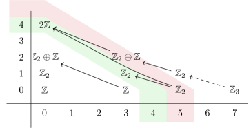
Figure 11: $E_{2}$ page of the AHSS for $\Omega^{\mathrm{Spin}}_{*}(PSU(n))$ associated to the fibration (64). We have shaded the entries with total degree four (green) and five (red).

We can repeat the above procedure with the fibration

(66)

Since $B\mathbb{Z}_{n}=K(\mathbb{Z}_{n},1)$, proceeding as above we obtain a fibration

(67)

Computing the homology of $K(\mathbb{Z}_{n},2)$ is more laborious. Although a general algorithm to compute these in principle can be found in MR0087935 , we will only discuss the cases $n=p^{k}$, for $p$ prime. The main tool we will use is the following theorem (see POINTETTISCHLER19971113 ; TischlerPhD ) that gives $H_{i}(K(\mathbb{Z}_{p^{k}},2),\mathbb{Z})$ as follows:

$$H_{i}(K(\mathbb{Z}_{p^{k}},2),\mathbb{Z}) =M_{1}\oplus M_{2},\quad\text{where}$$

$$M_{1} =\begin{cases}0&\text{if}\quad i\in 2\mathbb{Z}+1,\\ \mathbb{Z}_{p^{f+s}}&\text{if}\quad i\in 2\mathbb{Z}\quad\text{and}\quad\frac{i}{2}=rp^{s},\end{cases}$$ (68)

where $p$ does not divide $r$. $M_{2}$ is a finite group whose exponent is bounded above by $S(i)$, where

$$S(i) =\prod_{q\in\mathcal{P}(i)}q^{\varphi(q,i)},\quad\mathcal{P}(i)=\left\{q\quad\text{prime s.t.}\quad q\leq\frac{i}{2}\right\},$$

$$\varphi(q,i) =\text{max}\left\{1,\left\lfloor\log_{q}\frac{i}{2q}\right\rfloor+1\right\}.$$ (69)

Using these results, we can compute the homology groups $H_{i}(K(\mathbb{Z}_{p^{k}},2),\mathbb{Z})$:

$$\begin{array}[]{c|c|c|c|c|c|c|c|c}i&0&1&2&3&4&5&6&7\\ \hline\cr H_{i}&\mathbb{Z}&0&\mathbb{Z}_{2^{k}}&0&A_{p^{k}}\oplus\begin{cases}\mathbb{Z}_{2^{k+1}}&p=2,\\ \mathbb{Z}_{p^{k}}&p\neq 2\end{cases}&B_{p^{k}}&C_{p^{k}}\oplus\begin{cases}\mathbb{Z}_{3^{k+1}}&p=3,\\ \mathbb{Z}_{p^{k}}&p\neq 2\end{cases}&D_{p^{k}}\end{array}$$ (70)

Here, $A$ and $B$ are groups of exponent $\leq 2$; this means that they are of the form $h\mathbb{Z}_{2}$, for some integer $h$, and $C$ and $D$ have exponent $\leq 6$, meaning that all the elements have degree $\leq 6$.

We will now discuss the case at prime 2 and higher primes separately:

3.5.1 $p=2$

In this case, we can use the computer program described in ClementPhD to compute $A,B,C,D$ explictly. To get the homology with $\mathbb{Z}_{2}$ coefficients, we use the universal coefficient theorem. This produces some extensions of the form $e(\mathbb{Z}_{2},\mathbb{Z}_{2})$, which we know to be trivial since homology groups with coefficients in a ring $R$ must be $R$-modules (and $\mathbb{Z}_{4}$ is not a $\mathbb{Z}_{2}$-module). We obtain

$$\begin{array}[]{c|ccccccccc}i&0&1&2&3&4&5&6&7&8\\ \hline\cr H_{i}(K(\mathbb{Z}_{2^{k}},2),\mathbb{Z})&\mathbb{Z}&0&\mathbb{Z}_{2^{k}}&0&\mathbb{Z}_{2^{k+1}}&\mathbb{Z}_{2}&\mathbb{Z}_{2^{k}}&\mathbb{Z}_{2}&\mathbb{Z}_{2}\oplus\mathbb{Z}_{2^{k+2}}\\ H_{i}(K(\mathbb{Z}_{2^{k}},2),\mathbb{Z}_{2})&\mathbb{Z}_{2}&0&\mathbb{Z}_{2}&\mathbb{Z}_{2}&\mathbb{Z}_{2}&2\mathbb{Z}_{2}&2\mathbb{Z}_{2}&2\mathbb{Z}_{2}&3\mathbb{Z}_{2}\end{array}$$ (71)

From this, we can construct the spectral sequence depicted in figure 12.

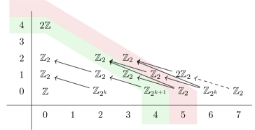
Figure 12: $E_{2}$ page of the AHSS for $\Omega^{\mathrm{Spin}}_{*}(PSU(n))$ associated to the fibration (67), where $n=2^{k}$.

Requiring the results of the two spectral sequences in figures 11 and 12 to be compatible, we can compute the relevant bordism groups up to third degree:

$$\begin{array}[]{c|cccc}i&0&1&2&3\\ \hline\cr\Omega^{\mathrm{Spin}}_{i}(PSU(2^{k}))&\mathbb{Z}&\mathbb{Z}_{2}&\mathbb{Z}_{2}\oplus\mathbb{Z}_{2^{k}}&0\end{array}$$ (72)

Unknown differentials prevent us from proceeding any further. Note that in this case, we cannot use the result described around (27), since we are using the AHSS for a nontrivial fibration.

3.5.2 $p\neq 2$

In this case, we can also determine the groups $A,B,C,D$, using Serre’s spectral sequence for the fibration Hatcher:478079

(73)

where $*$ is a contractible space. As we know (see appendix C), the reduced integer homology of $K(\mathbb{Z}_{n},1)=B\mathbb{Z}_{n}$ localizes at odd degree, where it is $\mathbb{Z}_{n}$. In fact, direct application of the universal coefficient theorem tells us that, in the range $i\leq 5$ and for odd $p$, $H_{i}(K(\mathbb{Z}_{p^{k}},2),\mathbb{Z}_{n})=\mathbb{Z}_{n}$ with the sole exception of $i=1$, which vanishes. As a result, in the AHSS associated to the fibration (73), depicted in figure 13, there can be no nonvanishing differentials acting on $A,B$ for $p\neq 2$, and the same holds for $C,D$ for $p\neq 2,3$. Since the resulting space is contractible, we can conclude that $A=B=0$ for $p\neq 2$ and $C=D=0$ for $p\neq 2,3$.

Figure 13: $E_{2}$ page of the Serre spectral sequence associated to the fibration (73).

We can now compute the homology with mod 2 coefficients, which turns out to be extremely simple:

$$\begin{array}[]{c|cccccc}i&0&1&2&3&4&5\\ \hline\cr H_{i}(K(\mathbb{Z}_{p^{k}},2),\mathbb{Z})&\mathbb{Z}&0&\mathbb{Z}_{p^{k}}&0&\mathbb{Z}_{p^{k}}&0\\ H_{i}(K(\mathbb{Z}_{p^{k}},2),\mathbb{Z}_{2})&\mathbb{Z}&0&0&0&0&0\end{array}$$ (74)

The AHSS associated to (67) is depicted in figure 14.

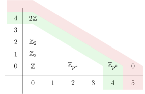
Figure 14: $E_{2}$ page of the AHSS for $\Omega^{\mathrm{Spin}}_{*}(PSU(n))$ associated to the fibration (67), for $n=p^{k}$ where $p$ is an odd prime.

Comparison with (64) allows us to compute the bordism groups up to degree five in this case:

$$\begin{array}[]{c|cccccc}i&0&1&2&3&4&5\\ \hline\cr\Omega^{\mathrm{Spin}}_{i}(PSU(p^{k}))&\mathbb{Z}&\mathbb{Z}_{2}&\mathbb{Z}_{2}\oplus\mathbb{Z}_{2^{k}}&0&2\mathbb{Z}&0\end{array}$$ (75)

We see that there are no new anomalies in four dimensions.

3.6 Orthogonal groups

3.6.1 $SO(3)$

We now discuss $SO(n)$ groups, starting with the case $n=3$. While $SO(3)\equiv PSU(2)$, and thus it is already covered by our discussion in section 3.5 above, we will analyze it again using different techniques as a warm-up exercise towards the case of general $n$.

Using the results in Feshbach for $H^{*}(BSO(n),\mathbb{Z})$, together with the universal coefficient theorem, we find

$$\begin{array}[]{c|ccccccccc}n&0&1&2&3&4&5&6&7&8\\ \hline\cr H^{n}(BSO(3),\mathbb{Z})&\mathbb{Z}&0&0&\mathbb{Z}_{2}&\mathbb{Z}&0&\mathbb{Z}_{2}&\mathbb{Z}_{2}&\mathbb{Z}\\ H_{n}(BSO(3),\mathbb{Z})&\mathbb{Z}&0&\mathbb{Z}_{2}&0&\mathbb{Z}&\mathbb{Z}_{2}&\mathbb{Z}_{2}&0&\mathbb{Z}\oplus\mathbb{Z}_{2}\\ H^{n}(BSO(3),\mathbb{Z}_{2})&\mathbb{Z}_{2}&0&\mathbb{Z}_{2}&\mathbb{Z}_{2}&\mathbb{Z}_{2}&\mathbb{Z}_{2}&2\mathbb{Z}_{2}&\mathbb{Z}_{2}&2\mathbb{Z}_{2}\\ H_{n}(BSO(3),\mathbb{Z}_{2})&\mathbb{Z}_{2}&0&\mathbb{Z}_{2}&\mathbb{Z}_{2}&\mathbb{Z}_{2}&\mathbb{Z}_{2}&2\mathbb{Z}_{2}&\mathbb{Z}_{2}&2\mathbb{Z}_{2}\end{array}$$ (76)

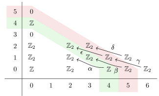
Figure 15: $E_{2}$ page of the AHSS for $\Omega^{\mathrm{Spin}}_{*}(BSO(3))$. We have omitted some terms which are not relevant for the computation of $E_{\infty}$ up to total degree 5, we have shaded the entries of total degree 4 and 5, and indicated the potentially non-vanishing differentials of degree 2.

From here it is straightforward to write the Atiyah-Hirzebruch spectral sequence, the result is shown in figure 15. We will compute the bordism groups $\Omega_{4}^{\mathrm{Spin}}(BSO(3))$ and $\Omega_{5}^{\mathrm{Spin}}(BSO(3))$. We see that in this range there are a number of potentially non-vanishing differentials, so we will need extra information to proceed. First, from TeichnerPhD ; Teichner , we have that

$$d_{2}^{(r,0)}\colon E_{2}^{(r,0)}\to E_{2}^{(r-2,1)} =\mathrm{Sq}^{2}_{*}\circ\rho_{2}$$ (77)

$$d_{2}^{(r,1)}\colon E_{2}^{(r,1)}\to E_{2}^{(r-2,2)} =\mathrm{Sq}^{2}_{*}$$ (78)

where $\mathrm{Sq}_{*}^{2}$ is the dual of $\mathrm{Sq}^{2}$, and $\rho_{2}\colon H_{i}(M,\mathbb{Z})\to H_{i}(M,\mathbb{Z}_{2})$ is reduction of coefficients modulo 2. More precisely, it is the map induced in homology from the exact coefficient sequence $0\to\mathbb{Z}\to\mathbb{Z}\to\mathbb{Z}_{2}\to 0$. This induces the long exact sequence

$$\ldots\to H_{i}(M,\mathbb{Z})\xrightarrow{\,\cdot 2\,}H_{i}(M,\mathbb{Z})\xrightarrow{\,\rho_{2}\,}H_{i}(M,\mathbb{Z}_{2})\to H_{i-1}(M,\mathbb{Z})\to\ldots$$ (79)

For our purposes we are interested in the action of $\rho_{2}$ on $H_{i}(BSO(3),\mathbb{Z})$ with $i\in\{4,5,6\}$. These are all generated by a single generator $e_{i}$. Exactness of (79) then immediately implies $\rho_{2}(e_{4})=m_{4}$ and $\rho_{2}(e_{5})=m_{5}$, where we have denoted by $m_{i}$ the generators of $H_{i}(BSO(3),\mathbb{Z}_{2})$. The last remaining case, $\rho_{2}(e_{6})$ is more subtle, since $H_{6}(BSO(3),\mathbb{Z}_{2})=\mathbb{Z}_{2}\oplus\mathbb{Z}_{2}$. All we know from exactness of (79) is that $\rho_{2}$ is injective when acting on $H_{6}(BSO(3),\mathbb{Z})$, but not which combination of generators it maps to.

We now pass to the evaluation of the dual Steenrod squares

$$\mathrm{Sq}_{*}^{2}\colon H_{i}(M,\mathbb{Z}_{2})\to H_{i-2}(M,\mathbb{Z}_{2}).$$ (80)

Recall that these are defined by

$$\bigl{\langle}\mathrm{Sq}^{2}a,b\bigr{\rangle}=\bigl{\langle}a,\mathrm{Sq}_{*}^{2}b\bigr{\rangle}$$ (81)

for all $a\in H^{i}(M,\mathbb{Z}_{2})$ and $b\in H_{i+2}(M,\mathbb{Z}_{2})$, and the pairing $\bigl{\langle}-,-\bigr{\rangle}$ is the Kronecker pairing. Notice that this definition makes sense since $H^{i}(M,\mathbb{Z}_{2})=\operatorname{Hom}_{\mathbb{Z}_{2}}(H_{i}(M,\mathbb{Z}_{2}))$, as remarked above, so there is a natural non-degenerate pairing.

In order to proceed, we need to know the action of the Steenrod squares on the cohomology of $BSO(3)$. This is a classic result, originally due to Wu WuSteenrod (see also §8 of Borel1953 ). The $\mathbb{Z}_{2}$-valued cohomology of $BSO(n)$ is the finitely generated ring on $n-1$ variables

$$H^{*}(BSO(n),\mathbb{Z}_{2})=\mathbb{Z}_{2}[w_{2},\ldots,w_{n}]\,.$$ (82)

The Steenrod squares act on the generators of this ring as

$$\mathrm{Sq}^{i}w_{j}=\sum_{t=0}^{i}\begin{pmatrix}j-i+t-1\\ t\end{pmatrix}w_{i-t}w_{j+t}$$ (83)

for $i\leq j$, and 0 otherwise. For the cases at hand, this implies

$$\mathrm{Sq}^{1}w_{2}=w_{3}\quad,\quad\mathrm{Sq}^{2}w_{2}=w_{2}^{2}\quad,\quad\mathrm{Sq}^{1}w_{3}=0\quad\text{and}\quad\mathrm{Sq}^{2}w_{3}=w_{2}\smile w_{3}\,.$$ (84)

Steenrod squares of products of $w_{i}$ can then be derived via the Cartan formula (30d).

Let us now finally determine the relevant differentials. We start with $\alpha$. The relevant Steenrod square in cohomology is

$$\alpha_{*}\colon H^{2}(BSO(3),\mathbb{Z}_{2})\to H^{4}(BSO(3),\mathbb{Z}_{2})$$ (85)

and since $w_{2}$ generates $H^{2}(BSO(3),\mathbb{Z}_{2})$ this gives $\alpha_{*}(w_{2})=\mathrm{Sq}^{2}(w_{2})=w_{2}^{2}$. Since $w_{2}^{2}$ generates $H^{4}(BSO(3),\mathbb{Z}_{2})$ we conclude that the dual map

$$\mathrm{Sq}_{*}^{2}\colon H_{4}(BSO(3),\mathbb{Z}_{2})\to H_{2}(BSO(3),\mathbb{Z}_{2})$$ (86)

is the nontrivial one, sending the generator to the generator. As argued above, $\rho_{2}$ acts non-trivially on $H_{4}(BSO(3),\mathbb{Z})$, so we find that $\alpha$ itself is non-trivial. A very similar argument gives that $\beta$ is non-trivial, since $\mathrm{Sq}^{2}$ maps the generator $w_{3}$ of $H^{3}(BSO(3),\mathbb{Z}_{2})$ to the generator $w_{2}w_{3}$ of $H^{5}(BSO(3),\mathbb{Z}_{2})$, and $\rho_{2}$ acts non-trivially on $H_{5}(BSO(3),\mathbb{Z}_{2})$.

We now proceed to the differential $\epsilon$. The structure is very analogous to $\alpha$, except for the fact that we do not need to reduce coefficients. We conclude that it is non-vanishing, since $\mathrm{Sq}_{*}^{2}$ acts non-trivially on the relevant homology groups. Notice that since $\epsilon$ is injective, we find (since $\epsilon\circ\gamma=0$) that $\gamma$ vanishes. We can obtain in this way some information about $\rho_{2}$ acting on $H_{6}(BSO(3),\mathbb{Z})$. We have

$$\mathrm{Sq}^{2}(w_{2}^{2})=2\mathrm{Sq}^{2}w_{2}\smile w_{2}+\mathrm{Sq}^{1}w_{2}\smile\mathrm{Sq}^{1}w_{2}=w_{3}^{2}$$ (87)

which is one of the generators of $H^{6}(BSO(3),\mathbb{Z}_{2})$, the other being $w_{2}^{3}$. From here we learn that the dual Steenrod square is given by

$$\mathrm{Sq}_{*}^{2}\omega_{3}^{2}=\omega_{2}^{2}\quad;\quad\mathrm{Sq}_{*}^{2}\omega_{2}^{3}=0\,,$$ (88)

where by $\omega_{i}^{k}$ we mean the dual in homology of $w_{i}^{k}$. Since $\gamma=\mathrm{Sq}_{*}^{2}\circ\rho_{2}=0$, this implies that $\rho_{2}(m)=\omega_{2}^{3}$ or 0, with $m$ the generator of $H_{6}(BSO(3),\mathbb{Z})$. We have argued above that the map is injective, so we conclude $\rho_{2}(m)=\omega_{2}^{3}$.

Finally, we need to analyze the differential $\delta\colon H_{5}(BSO(3),\mathbb{Z}_{2})\to H_{3}(BSO(3),\mathbb{Z}_{2})$. By the same argument as for $\beta$, we conclude that this map is an isomorphism.

The end result of this discussion is that all of the $\mathbb{Z}_{2}$ factors of $E_{2}$ of total degree 4 or 5 vanish in $E_{3}$, and thus

$$\Omega^{\mathrm{Spin}}_{4}(BSO(3))=\mathbb{Z}\oplus\mathbb{Z}\quad;\quad\Omega_{5}^{\mathrm{Spin}}(BSO(3))=0\,.$$ (89)

Figure 16: $E_{2}$ page of the AHSS for $\Omega^{\mathrm{Spin}}_{*}(BSO(3))$. We have omitted the terms which are not relevant for the computation of entries in $E_{\infty}$ of total degree 6, and we have shaded the entries of total degree 6.

Let us also compute $\Omega_{6}^{\mathrm{Spin}}(BSO(3))$ via the AHSS in figure 16. The analysis can be performed as in the previous case.

The $\delta$ and $\gamma$ maps have been analyzed before, with the conclusion that $\delta$ was a bijection, and $\gamma=0$. The new maps are $\zeta$, $\eta$ and $\theta$. Let us start with $\eta$, which is the dual of the Steenrod square $\mathrm{Sq}^{2}\colon H^{4}(BSO(3),\mathbb{Z}_{2})\to H^{6}(BSO(3),\mathbb{Z}_{2})$. This was computed in (88) above, with the result that the map is surjective.

In order to compute $\zeta$, notice first that from the $0\to\mathbb{Z}\to\mathbb{Z}\to\mathbb{Z}_{2}\to 0$ short exact sequence, and $H_{7}(BSO(3),\mathbb{Z})=0$, we obtain that

$$\ldots\to H_{8}(BSO(3),\mathbb{Z})\xrightarrow{\,\cdot 2\,}H_{8}(BSO(3),\mathbb{Z})\xrightarrow{\,\rho_{2}\,}H_{8}(BSO(3),\mathbb{Z}_{2})\to 0$$ (90)

is exact, so $\rho_{2}$ is surjective when acting on $H_{8}(BSO(3),\mathbb{Z})$. We also need

$$\mathrm{Sq}^{2}\colon H^{6}(BSO(3),\mathbb{Z}_{2})\to H^{8}(BSO(3),\mathbb{Z}_{2}).$$ (91)

The first group is generated by $w_{2}^{3}$ and $w_{3}^{2}$, while the second is generated by $w_{2}^{4}$ and $w_{2}\smile w_{3}^{2}$. Using (30d) we find

$$\begin{split}\mathrm{Sq}^{2}w_{2}^{3}&=w_{2}\smile\mathrm{Sq}^{2}w_{2}^{2}+\mathrm{Sq}^{1}w_{2}\smile\mathrm{Sq}^{1}w_{2}^{2}+\mathrm{Sq}^{2}w_{2}\smile w_{2}^{2}\\ &=w_{2}\smile w_{3}^{2}+w_{3}\smile(2w_{2}w_{3})+w_{2}^{4}\\ &=w_{2}\smile w_{3}^{2}+w_{2}^{4}\,.\end{split}$$ (92)

Similarly

$$\mathrm{Sq}^{2}w_{3}^{2}=2w_{3}\mathrm{Sq}^{2}w_{3}+(\mathrm{Sq}^{1}w_{3})^{2}=0$$ (93)

where we have used $\mathrm{Sq}^{1}w_{3}=0$ in $BSO(3)$. Dualizing:

$$\mathrm{Sq}_{*}^{2}\omega_{2}^{4}=\mathrm{Sq}_{*}^{2}(\omega_{2}\omega_{3}^{2})=\omega_{2}^{3}$$ (94)

using the same notation for the dual homology generators as above. As a small check, note that $\eta\circ\zeta=0$, as it should. (And more precisely, $\ker\eta=\operatorname{im}\zeta$, so $E_{3}^{(6,1)}=0$.)

Finally, we need to compute $\theta\colon H_{7}(BSO(3),\mathbb{Z}_{2})\to H_{5}(BSO(3),\mathbb{Z}_{2})$. The action of $\mathrm{Sq}^{2}$ on the generator of $H^{5}(BSO(3),\mathbb{Z}_{2})$ is easily found to be

$$\begin{split}\mathrm{Sq}^{2}w_{2}w_{3}&=w_{2}\smile\mathrm{Sq}^{2}w_{3}+\mathrm{Sq}^{1}w_{2}\smile\mathrm{Sq}^{1}w_{3}+\mathrm{Sq}^{2}w_{2}\smile w_{3}\\ &=2w_{2}^{2}\smile w_{3}=0\end{split}$$ (95)

using again $\mathrm{Sq}^{1}w_{3}=0$ and the basic relations (84). So the conclude $\theta=0$.

At this point we run out of technology to compute the relevant differentials. In particular, since we find $E_{3}^{(5,2)}=E_{2}^{(5,2)}=\mathbb{Z}_{2}$, there is a potentially non-vanishing differential $d_{3}\colon E_{3}^{(5,2)}\to E_{3}^{(2,4)}$ that we reach before we fully stabilize. There is some discussion in TeichnerPhD about what these differentials are, but without going into that, we can conclude in any case that $\Omega_{6}^{\mathrm{Spin}}(BSO(3))$ is either $E_{2}^{(6,0)}=\mathbb{Z}_{2}$, or (if the differential vanishes) some extension of $\mathbb{Z}_{2}$ by $\mathbb{Z}_{2}$. It would be rather interesting to characterize what this means, and whether it signals some anomaly for the five-dimensional theory.

One observation that may be helpful here is that there is a simple bordism invariant that characterizes $H^{6}(BSO(3),\mathbb{Z})=\mathbb{Z}_{2}$. Note that since $H^{5}(BSO(3),\mathbb{Z})=0$, we have an exact sequence

$$0\to H^{5}(BSO(3),\mathbb{Z}_{2})\xrightarrow{\,\beta\,}H^{6}(BSO(3),\mathbb{Z})\to\ldots$$ (96)

We have $H^{5}(BSO(3),\mathbb{Z}_{2})=H^{6}(BSO(3),\mathbb{Z})=\mathbb{Z}_{2}$, so we can identify the generator of $H^{6}(BSO(3),\mathbb{Z})$ with $\beta(e)$, where $e$ is the generator of $H^{5}(BSO(3),\mathbb{Z}_{2})$ and $\beta$ is the Bockstein map. So a natural bordism invariant of six-manifolds is $\bigl{\langle}\beta(e),M\bigr{\rangle}$ where $M$ is the fundamental class of the manifold.

3.6.2 $SO(n)$

We can use the above results to compute $\Omega_{5}^{\mathrm{Spin}}(BSO(n))$, for $n\geq 3$ as well. The AHSS is displayed in figure 17, where we have also illustrated the relevant differentials.

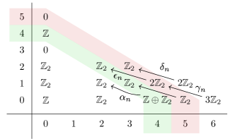
Figure 17: $E^{2}$ page of the AHSS for $\Omega^{\mathrm{Spin}}_{*}(BSO(n))$, for $n\geq 8$. The only differential without a label is $\beta_{n}$.

The structure is very similar to that of figure 15, but the groups are different. $\delta_{n}$ and $\epsilon_{n}$ are again given simply in terms of dual Steenrod squares; they are again nonvanishing. To analyze $\alpha_{n},\beta_{n}$ and $\gamma_{n}$ we need again to know the action of $\rho$ on $H_{i}(BSO(n),\mathbb{Z})$ for $i=4,5,6$. From the long exact sequence in homology, we again know that $\rho_{4}$ is surjective, and sends both generators of $\mathbb{Z}\oplus\mathbb{Z}_{2}$ to generators. This means that $\alpha_{n}$ is again nontrivial. Likewise, we know that the image and kernel of $\rho_{5}$ are $\mathbb{Z}_{2}$, and that the image of $\rho_{6}$ is $3\mathbb{Z}_{2}$, but we need to know the precise action on generators. Fortunately, we can leverage our knowledge of the $SO(3)$ case to obtain the answer for $SO(n)$ as well. To do this, note that the inclusion $SO(3)\subset SO(n)$ induces the following commutative diagram, where the entries are the corresponding chain complexes,

(97)

which induces a commutative diagram in homology rotman1998introduction

(98)

Here, $i_{*}$ are the natural maps in homology induced by the inclusion. This commutative diagram in turn allows us to compute $\text{im}(\rho_{SO(n)})=\text{ker}(\beta_{SO(n)})$ by constructing $\beta^{\prime}_{SO(n)}=\iota_{*}\circ\beta^{\prime}_{SO(3)}$.

$H_{5}(BSO(n),\mathbb{Z}_{2})$ is generated by $\xi_{3}\xi_{2},\xi_{5}$, the Kronecker dual basis to $w_{3}w_{2},w_{5}$, and as above $H_{5}(BSO(3),\mathbb{Z}_{2})$ is generated by $\omega_{3}\omega_{2}$. Since in cohomology we have $\iota^{*}(w_{3}w_{2})=w_{3}w_{2}$, $\iota^{*}(w_{5})=0$ 10.2307/2044298 , we obtain

$$\iota_{*}(\omega_{3}\omega_{2})=\xi_{3}\xi_{2}$$ (99)

Since in this case $\beta^{\prime}_{SO(3)}=0$, the commutative diagram means that $\beta^{\prime}_{SO(n)}(\xi_{3}\xi_{2})=0$. This means that the image of the reduction modulo 2 map is generated by $\xi_{3}\xi_{2}$, and therefore that the differential $\beta_{n}$ is nonvanishing.

$H_{6}(BSO(n),\mathbb{Z}_{2})$ is generated by $\xi_{2}^{3}\xi_{3}^{2},\xi_{4}\xi_{2},\xi_{6}$, the Kronecker dual basis to the Stiefel-Whitney classes $w_{2}^{3},w_{3}^{2},w_{2}w_{4},w_{6}$. In cohomology we have $\iota^{*}(w_{2}^{3})=w_{2}^{3}$, $\iota^{*}(w_{3}^{2})=w_{3}^{2}$, we have, in the same notation as above,

$$\iota_{*}(\omega_{2}^{3})=\xi_{2}^{3},\quad\iota_{*}(\omega_{3}^{2})=\xi_{3}^{2}.$$ (100)

We also have $\beta^{\prime}_{SO(3)}(\omega_{2}^{3})=0$, $\beta^{\prime}_{SO(3)}(\omega_{3}^{2})=\omega_{3}\omega_{2}$, which combined with (99) means that $\text{ker}(\beta_{SO(n)}^{\prime})$ is generated by $\xi_{2}^{3},\xi_{6},\xi_{4}\xi_{2}$. This is also the image of the reduction modulo 2 map, so we can compute the $\gamma_{n}$ explicitly, to be the $\mathbb{Z}_{2}$ generated by $\xi_{4}$.

Combining all this, we get

$$\Omega^{\mathrm{Spin}}_{4}(BSO(n))=e(\mathbb{Z},\mathbb{Z}\oplus\mathbb{Z}_{2}),\quad\Omega^{\mathrm{Spin}}_{5}(BSO(n))=0.$$ (101)

Comparing with (89), we see that we get an extra $\mathbb{Z}_{2}$ factor. Presumably, this is measured by $\int w_{4}$.

3.6.3 $Spin(n)$

We can compute the $Spin(n)$ bordism groups in the same way as above. First, we need the homology groups, which are (for $n\geq 8$) 10.2307/2044298 ; 10.2307/24893350 ; QUILLEN1971 ; kono1986

$$\begin{array}[]{c|ccccccccccc}n&0&1&2&3&4&5&6&7&8\\ \hline\cr H_{i}(BSpin(n),\mathbb{Z})&\mathbb{Z}&0&0&0&\mathbb{Z}&0&\mathbb{Z}_{2}&0&2\mathbb{Z}\\ H_{i}(BSpin(n),\mathbb{Z}_{2})&\mathbb{Z}_{2}&0&0&0&\mathbb{Z}_{2}&0&\mathbb{Z}_{2}&\mathbb{Z}_{2}&2\mathbb{Z}_{2}\end{array}$$ (102)

With these we can construct the spectral sequence shown in figure 18. Since we have $H_{5}(BSpin(n),\mathbb{Z})=0$, the reduction modulo 2 is an isomorphism. To compute the relevant Steenrod square, we can use the result QUILLEN1971 ; 2009arXiv0904.0800K that the cohomology with $\mathbb{Z}_{2}$ coefficients of $BSpin(n)$ can be obtained from that of $BSO(n)$ via the pullback associated to the map $f:BSpin(n)\rightarrow BSO(n)$. Now, $H_{i}(BSO(n),\mathbb{Z}_{2})$ is a polynomial $\mathbb{Z}_{2}$ ring generated by the Stiefel-Whitney classes, with $w_{1}=0$. The pullback map sends to zero the classes $v_{k}=\mathrm{Sq}^{2^{k}}\ldots\mathrm{Sq}^{1}w_{2}$, where $k\leq h-1$ and $h$ is the so-called Radon-Hurwitz number, which is $\geq 9$ for $n\geq 8$.

Since $v_{0}=w_{2}$, $v_{1}=w_{3}$, the generator of $H^{4}(BSpin(n),\mathbb{Z}_{2})$ is just $f^{*}(w_{4})$, and the generator of $H^{6}(BSpin(n),\mathbb{Z}_{2})$ is $f^{*}(w_{6})$ . By functoriality of the Steenrod square and Wu’s formula (83),

$$\mathrm{Sq}^{2}(f^{*}w_{4})=f^{*}(\mathrm{Sq}^{2}(w_{4}))=f^{*}(w_{6}+w_{4}\smile w_{2})=f^{*}(w_{6})\,,$$ (103)

so the differential shown in figure 18 is nontrivial. As a result, $\Omega_{5}^{\mathrm{Spin}}(BSpin(n))=0$. In particular, this means that the $Spin(10)$ GUT is free of Dai-Freed anomalies.

Figure 18: $E_{2}$ page of the AHSS for $\Omega^{\mathrm{Spin}}_{*}(BSpin(n))$, for $n\geq 8$.

3.7 Exceptional groups

We can also compute the relevant bordism groups of exceptional groups by replacing $BG$ with a sufficiently close space which is better understood. The familiar case is $BE_{8}$, which up to degree 15 has the same homology structure as $K(\mathbb{Z},4)$ Witten:1985bt ; Edwards . Let us first review the general argument in some detail, following Stong-11 .

Suppose we have a map $f:A\rightarrow X$. Since bordism is a generalized homology theory, we have a long exact sequence

(104)

The important point is that the relative bordism groups $\Omega_{d}^{\mathrm{Spin}}(X,A)$ can also be computed via an AHSS with second page $E^{2}_{p,q}=H_{p}(X,A;\Omega^{\mathrm{Spin}}_{q}(\mathrm{pt}))$. We will be interested in the particular case where the induced map $f_{*}:\pi_{k}(A)\rightarrow\pi_{k}(X)$ is an isomorphism for all $k\leq n$. Then $\pi_{k}(X,A)=0$ for $k\leq n$, and by the relative version of Hurewicz’s theorem Hatcher:478079 , $H_{k}(X,A)=0$ for $k\leq n$. The lowest corner of the AHSS is trivial, proving that $\Omega_{k}^{\mathrm{Spin}}(X,A)$ for $k\leq n$. Then (104) proves that $\Omega_{d}^{\mathrm{Spin}}(A)=\Omega_{d}^{\mathrm{Spin}}(X)$ for $d<n$, so that we may replace $X$ by $A$ as far as low-dimensional bordisms are concerned.

Now, for any CW complex $X$, one can construct a Postnikov tower Hatcher:478079 . This is a family of spaces $X_{n}$ such that $\pi_{k}(X_{n})=\pi_{k}(X)$ for $k\leq n$, $\pi_{k}(X_{n})=0$ otherwise. There is an inclusion $X\rightarrow X_{n}$ which induces a isomorphism in the first $n$ homotopy groups. Combining with the above, we reach the conclusion that, if we want to compute the bordism groups of some space $X$ up to a finite degree $n$, we may replace it with the $(n+1)$-th floor $X_{n+1}$ of the Postnikov tower.

Now consider the classifying space for $BG$, where $G$ is any exceptional group. In fact, it is true for all exceptional groups that $\pi_{4}(BG)=\mathbb{Z}$ and $\pi_{i}(BG)=0$ for $i\leq 6$. So the sixth term in the Postnikov tower for $BG$, $(BG)_{6}$, has homotopy groups $\pi_{4}((BG)_{6})=\mathbb{Z}$, and 0 otherwise. This means that $(BG)_{6}$ is by definition a presentation of the Eilenberg-MacLane space $K(\mathbb{Z},4)$. This is turn implies that $\Omega_{i}^{\mathrm{Spin}}(BG)=\Omega_{i}^{\mathrm{Spin}}(K(\mathbb{Z},4))$ for $i\leq 5$. We can then immediately apply the result in Stong-11 , and conclude

$$\Omega_{5}^{\mathrm{Spin}}(BG)=0$$ (105)

for $G$ any exceptional group.

The same reasoning works for higher bordism groups whenever we have $\pi_{4}(BG)=\mathbb{Z}$ and $\pi_{i}(BG)=0$ otherwise for $i\leq d$, with $d$ large enough. For instance, for $G=E_{7}$ or $G=E_{8}$ we have Stong-11

$$\tilde{\Omega}_{8}^{\mathrm{Spin}}(BG)=\mathbb{Z}\oplus\mathbb{Z}\qquad;\qquad\tilde{\Omega}_{9}^{\mathrm{Spin}}(BG)=\mathbb{Z}_{2}\qquad;\qquad\tilde{\Omega}_{10}^{\mathrm{Spin}}(BG)=\mathbb{Z}_{2}\oplus\mathbb{Z}_{2}\,,$$ (106)

so for these groups we have the possibility of global anomalies in $d=\{7,8,9\}$. (The eight dimensional case was analyzed in Garcia-Etxebarria:2017crf .) For $F_{4}$, the above results only for $i\leq 7$, so we can only analyze anomalies up to $d=7$.

4 Discrete symmetries and model building constraints

We now turn to anomalies of discrete symmetries. These have a long story, see e.g. Ibanez:1991hv ; Ibanez:1992ji ; Dreiner:2005rd ; Mohapatra:2007vd ; Lee:2011dya ; Nilles:2012cy ; Chen:2015aba among many others. Our goal will be to compute the Dai-Freed anomalies in various cases of interest, and compare the known results. The relevant bordism groups are nontrivial, but luckily have already been computed in the mathematical literature in the works of Gilkey bahri1987 ; GilkeyBook ; Gilkey1996 ; Gilkey1998 , who also provides the $\eta$ invariant for generators of the bordism groups. (Some information about the bordism groups can also be obtained via an AHSS sequence, as we have been doing above. However, in this case, the AHSS is not enough to fully determine the groups, due to a nontrivial extension problem. Still, we have included the calculation for $\mathbb{Z}_{n}$ in appendix C for the benefit of the curious reader.)

More concretely, we will now explore the Dai-Freed anomaly of the so-called spherical space form groups GilkeyBook . The main tool we will use is the fact that there are some bordism classes for which the $\eta$ invariants can be computed explicitly (for a discussion, see GilkeyBook ).

A spherical space form is a generalization of a lens space, defined as follows. Let $G$ be a finite group, and $\tau:G\rightarrow U(k)$ a fixed-point free representation of it. Then, define

$$M(\tau,G)\equiv S^{2k-1}/\tau(G).$$ (107)

For $G=\mathbb{Z}_{n}$, this is an ordinary lens space such as the ones employed in appendix C.

We are naturally interested in $\mathrm{Spin}$ and $\mathrm{Spin}^{c}$ manifolds. For $M(\tau,G)$ to have a $\mathrm{Spin}$ or $\mathrm{Spin}^{c}$ structure, we just need to find a $\mathrm{Spin}$ or $\mathrm{Spin}^{c}$ lift of the $\tau(G)$.

For the $\mathrm{Spin}$ case, we have canonical spin lifts of every $\tau(G)$ up to a sign. For these to be consistent, we need that $\det(\tau)$ extends to a representation of $G$ Gilkey1996 . A particularly simple case to ensure this is if $\tau(G)\subset SU(k)$, in which case the determinant is 1 and $M(\tau,G)$ is always spin. As noted in Gilkey1996 , there is no spin structure on $M(\tau,G)$ if $|G|$ is even and $k$ odd: a finite group with even order always has an element that squares to the identity, which in this case has to be represented by a fixed-point-free square root of the identity, which can only be $\text{diag}(-1,\ldots-1)$. For $k$ odd, this has determinant $-1$.

The main technical result in Gilkey1996 is that $M$ represents a nontrivial class of $\Omega_{d+1}^{\mathrm{Spin}}(BG)$, and the $\eta$ invariant of the Dirac operator in a representation $\rho$ of $G$ is given by

$$\eta(M(\tau,G),\rho)=\frac{1}{|G|}\sum_{\lambda\in G-\{1\}}\text{Tr}(\rho(\lambda))\frac{\sqrt{\text{det}(\tau(\lambda))}}{\text{det}(I-\tau(\lambda))}.$$ (108)

For the $\mathrm{Spin}^{c}$ case, the correct expression is instead GilkeyBook ; Gilkey1996

$$\eta(M(\tau,G),\rho)=\frac{1}{|G|}\sum_{\lambda\in G-\{1\}}\text{Tr}(\rho(\lambda))\frac{\text{det}(\tau(\lambda))}{\text{det}(I-\tau(\lambda))}.$$ (109)

Application of the above formulae is straightforward to a number of discrete groups of interest.

Finally, as pointed out in section 2.1.2, Dai-Freed constraints such as the ones we discuss here can sometimes be circumvented by mild modifications, such as adding Green-Schwarz couplings to the Lagrangian, or by coupling to a suitable topological quantum field theory. It turns out that there are several ways of doing this for discrete symmetries, which we discuss in subsection 4.6.

4.1 $\mathrm{Spin}-\mathbb{Z}_{n}$

The lens space $S^{2k-1}/\mathbb{Z}_{n}\equiv L^{k}(n)$ is not Spin for $n$ even and $k$ odd, but it is for both $k$ and $n$ odd. As a result, we can use (108) to compute $\eta$ invariants corresponding to some bordism class in $\Omega_{5}^{\mathrm{Spin}}(B\mathbb{Z}_{n})$, for $n$ odd. The formula (108) now becomes

$$\eta(L^{k}(n),\rho_{s})=\frac{1}{n}\sum_{\lambda\neq 1}\left(\lambda^{s}-1\right)\left(\frac{\sqrt{\lambda}}{\lambda-1}\right)^{k}\,.$$ (110)

In this formula $s$ is the $\mathbb{Z}_{n}$ charge of the fermion and $\lambda$ is a $n$-th root of unity. One has to be careful to define the square root in such a way that $(\sqrt{\lambda})^{n}=+1$, a convenient definition is $\sqrt{\lambda}=\lambda^{(n+1)/2}$.

As discussed in GilkeyBook , Section 4.5.1, for odd $n$ the bordism ring $\Omega_{5}^{\mathrm{Spin}}(B\mathbb{Z}_{n})$ is actually generated by only two elements, $L^{3}(n)$ and $\text{K3}\times L^{1}(n)$. This means that there are at most two independent Dai-Freed anomaly cancellation conditions. Furthermore, we have (see bahri1987 , Lemma 2.2, or APS-III ; GilkeyBook )

$$\eta(A\times B)=\text{index}(A)\eta(B)$$ (111)

which means that

$$\eta(\text{K3}\times L^{1}(n))=\text{index}(\text{K3})\eta(L^{1}(n))=2\eta(L^{1}(n)).$$ (112)

So we only need to apply formula (110). Using the expressions in GilkeyBook in terms of Todd polynomials we obtain, after some simplifications,

$$\sum_{i}\left[s_{i}^{3}-\frac{1}{4}(n^{2}+3)s_{i}\right] \equiv 0\mod 6n$$ (113a)

$$\sum_{i}s_{i} \equiv 0\mod n\,,$$ (113b)

where the $s_{i}$ are the $\mathbb{Z}_{n}$ charges of the fermions in the theory.

As for the even $n$ case, Gilkey1996 provides a different family of lens spaces which allow the computation of $\Omega_{5}^{\mathrm{Spin}}(B\mathbb{Z}_{2^{k}})$. These spaces depend on two parameters $a_{1},a_{2}$ on top of $k$. For these, the $\eta$ invariant is

$$\eta=2^{-k}\sum_{\lambda\neq 1}(\lambda^{s}-1)\frac{\lambda^{(a_{1}+a_{2})/2}(1-\lambda^{a_{1}+a_{2}})}{(1-\lambda^{a_{1}})^{2}(1-\lambda^{a_{2}})^{2}}.$$ (114)

Since the Chinese remainder theorem means that

$$\mathbb{Z}_{2^{k}m}\approx\mathbb{Z}_{2^{k}}\oplus\mathbb{Z}_{m},$$ (115)

we can compute some $\eta$ invariants representing factors of $\Omega_{5}^{\mathrm{Spin}}(B\mathbb{Z}_{n})$ for any $n$. These are not necessarily all of the $\eta$ invariants; there might be mixed anomalies between the different factors in (115).

We now apply the above anomaly cancellation conditions to some interesting cases such as $\mathbb{Z}_{3}$, where we obtain the constraint that the net number of $\mathbb{Z}_{3}$ fermions (counted $+1$ if they have charge $1\,\text{mod}\,3$, and $-1$ if they have $2\,\text{mod}\,3$) has to vanish modulo 9,

$$\sum_{\text{fermions}}s_{i}\quad\equiv\quad 0\,\text{mod}\,9,$$ (116)

and $\mathbb{Z}_{4}$, where the net number of $\mathbb{Z}_{4}$ fermions (counted $+1$ if they have charge $1\,\text{mod}\,4$, $-1$ if they have $3\,\text{mod}\,4$, and $0$ otherwise) must vanish modulo 4. For $\mathbb{Z}_{5}$, the net number has to vanish mod 5, where the fermions are counted as $+1$ if they have charge 1 or 3 mod 5, -1 if they have charge 2 or 4 mod 5, and 0 if their $\mathbb{Z}_{5}$ charge vanishes. For $\mathbb{Z}_{2}$ the bordism group vanishes. This means, for instance that R-parity in the MSSM is not anomalous.

On the other hand, if we have a $\mathbb{Z}_{n}$ bundle which can be embedded in a $U(1)$ where local anomalies cancel, then all Dai-Freed anomalies of the $\mathbb{Z}_{n}$ must vanish. This is because, as we computed in section 3.3, $\Omega_{5}^{\mathrm{Spin}}(BU(1))=0$, and the $\mathbb{Z}_{n}$ $\eta$ invariant can also be regarded as a $U(1)$ $\eta$ invariant, evaluated in a particular bundle whose transition functions lie in $\mathbb{Z}_{n}\subset U(1)$.

4.2 Baryon triality

The constraint (116) has phenomenological implications, as we will now see. Consider the $\mathbb{Z}_{3}$ baryon triality symmetry Ibanez:1991pr ; Dreiner:2005rd , commonly used to ensure proton stability in the MSSM. This is a symmetry under which the chiral superfields are charged as in table 1. The total charge mod 9, counted as above, is 3 per generation, so we need the number of generations to be a multiple of 3 in order for baryon triality to be anomaly-free. Note that the anomaly that we found for the $\mathbb{Z}_{3}$ symmetry implies that baryon triality cannot be embedded into an anomaly-free $U(1)$ as long as generation-independent $U(1)$ charges are considered: we have just seen that a $\mathbb{Z}_{3}$ subgroup of the $U(1)$ is anomalous for the case of a single generation, and introducing extra generations cannot make an anomalous $U(1)$ anomaly-free. If we allow for generation dependent $U(1)$ charges (but imposing that these $U(1)$ charges lead to generation-independent $\mathbb{Z}_{3}$ charges), then it is possible to cancel the anomaly with three generations.

	$Q$	$\bar{U}$	$\bar{D}$	$L$	$\bar{E}$	$H_{u}$	$H_{d}$
Triality	0	-1	1	-1	-1	1	1
Hexality	0	-2	-5	-5	1	5	5

Table 1: $\mathbb{Z}_{3}$ and $\mathbb{Z}_{6}$ charges of the MSSM chiral superfields under baryon triality and proton hexality. We use the conventions in Dreiner:2005rd .

The above analysis also extends to the proton hexality symmetry proposed in Dreiner:2005rd . Since $\mathbb{Z}_{6}\approx\mathbb{Z}_{2}\oplus\mathbb{Z}_{3}$, and $\Omega_{5}^{\mathrm{Spin}}(B\mathbb{Z}_{2})=0$ because of a Smith homomorphism, a $\mathbb{Z}_{6}$ discrete symmetry suffers from the same $\mathbb{Z}_{3}$ anomaly. The mod 3 reduction of the second row of table 1 is minus the first row, so proton hexality suffers from the same anomaly. Just as in the previous case, thanks to the fact that the Standard Model has three generations, this anomaly can be fixed via generation-dependent couplings; this indeed is what happens in section 9 of Dreiner:2005rd .

As discussed above, all the discrete anomaly constraints that we are discussing should be automatically satisfied whenever the $\mathbb{Z}_{n}$ can be embedded into a non-anomalous $U(1)$. In particular, the mod 9 condition should be obtainable from local anomaly cancellation conditions. Consider a $U(1)$ with charges $q_{i}=(3m_{i}+r_{i})$, where $m_{i}$ are integers and the $r_{i}$ are $-1,0,1$. As above, local anomaly imposes

$$\sum_{i}27(m_{i}^{3}+m_{i}^{2}r_{i})+9m_{i}r_{i}^{2}+r_{i}^{3}=0,\quad\sum_{i}m_{i}+r_{i}=0.$$ (117)

Because of the definition, $r_{i}^{3}=r_{i}$. Taking the first equation modulo 9, we obtain

$$\sum_{i}r_{i}\equiv 0\,\text{mod}\,9,$$ (118)

as advertised.

4.3 SM fermions and the topological superconductor

Here we discuss briefly one of the observations that led to this work: that the number of fermions per generation in the SM (including right handed neutrinos) is 16, which turns out to be the number of Majorana zero modes of a topological superconductor that cancels the Dai-Freed anomaly of time reversal. It turns out that the two facts can be nicely related if we assume a certain $\mathbb{Z}_{4}$ subgroup of $(B-L)$+ the SM gauge group to be gauged, as follows.

In the Standard model extended with right-handed neutrinos, there is a particular combination of hypercharge and $B-L$,

$$X\equiv-2Y+5(B-L),$$ (119)

such that the charges of all SM fermions under $X$ are of the form $q_{i}=4k_{i}+1$. This means that $q^{X}_{i}\,\text{mod}\,4$ is a $\mathbb{Z}_{4}$ charge under which every fermion has a charge of $1\,\text{mod}\,4$. For convenience, we have included the relevant representations of standard model fields in table 2.

SM field	$\mathbf{SU(3)}$	$\mathbf{SU(2)}$	$\mathbf{Y}$	$\mathbf{{B-L}}$	$\mathbf{X}$
$l^{c}_{L}$	$\mathbf{1}$	$\mathbf{2}$	$-3$	3	$21$
$q^{c}_{L}$	${\bar{\mathbf{3}}}$	$\mathbf{2}$	1	$-1$	-7
$l_{R}$	$\mathbf{1}$	$\mathbf{1}$	6	$-3$	-27
$u_{R}$	$\mathbf{3}$	$\mathbf{1}$	$-4$	1	$13$
$d_{R}$	$\mathbf{3}$	$\mathbf{1}$	2	1	1
$\nu_{R}$	$\mathbf{1}$	$\mathbf{1}$	0	$-3$	-15
$H$	$\mathbf{1}$	$\mathbf{2}$	3	0	-6

Table 2: Charge assignments of the fields in the Standard Model. All fermions are right-moving chiral Weyl fermions. We have rescaled the hypercharge $Y$ and $B-L$ such that all fields have integer charges. $H$ is the Higgs doublet. We have included a right-handed Majorana neutrino.

As discussed recently in Tachikawa:2018njr , in the presence of an extra $\mathbb{Z}_{4}$ symmetry, it is possible to make sense of fermions in manifolds that are not $\mathrm{Spin}$. More concretely, one can take the structure group to be $(\mathrm{Spin}\times\mathbb{Z}_{4})/\mathbb{Z}_{2}$, where the generator of the $\mathbb{Z}_{2}$ subgroup of $\mathbb{Z}_{4}$ and $(-1)^{F}$ are identified. This was called a $\mathrm{Spin}^{\mathbb{Z}_{4}}$ structure in Tachikawa:2018njr . Because of the above, the SM admits a $\mathrm{Spin}^{\mathbb{Z}_{4}}$ structure.

The same reference also constructs a version of the Smith homomorphism, along the same lines as in section 4.4.2 below, establishing that

$$\Omega_{4}^{\mathrm{Pin}^{+}}\approx\Omega_{5}^{\mathrm{Spin}^{\mathbb{Z}_{4}}}\,.$$ (120)

Physically, one can construct $\mathrm{Spin}^{\mathbb{Z}_{4}}$ bundles which contain domain walls on which 3d $\mathrm{Pin}^{+}$ fermions localize. For each 4d Weyl fermion with charge 1 modulo 4, we get one 3d $\mathrm{Pin}^{+}$ Majorana fermion.

Using $X$ defined in (119), we see that we reproduce this story once for each standard model fermion. Since the anomaly for the topological superconductor vanishes only when the number of Majorana fermions is a multiple of sixteen Witten:2015aba , we learn that the number of fermions in the standard model must be a multiple of sixteen for the $\mathbb{Z}_{4}$ symmetry to be anomaly-free. This is precisely the number of fermions in a generation of the standard model, once we include the right-handed neutrino.

As discussed above, if the above $\mathbb{Z}_{4}$ symmetry is assumed to embed into a $U(1)$ (in this case, the combination (119) of hypercharge and $B-L$), then the relevant bordism group becomes $\Omega^{\mathrm{Spin}^{c}}_{5}=0$, so the constraint that the number of fermions must be a multiple of 16 must already be implied by local anomaly cancellation. And indeed, in this case the anomaly cancellation conditions for $U(1)$ factors (coming from $\operatorname{Tr}(F_{U(1)}R^{2})=\operatorname{Tr}(F_{U(1)}^{3})=0$)

$$\sum_{i}q_{i}=\sum_{i}q_{i}^{3}=0$$ (121)

with $q_{i}$ the $U(1)$ charges of the fermions, imply that the total number of fermions $n_{F}$ is a multiple of 16, as follows. Define $p_{l}=\sum_{i}k_{i}^{l}$ (recall that we defined above $q_{i}=4k_{i}+1$). The first anomaly cancellation condition implies $n_{F}=-4p_{1}$, and the second is

$$0=n_{F}+12p_{1}+48p_{2}+64p_{3}=-2n_{F}+48p_{2}+64p_{3}\,,$$ (122)

which implies $n_{F}=8(3p_{2}+4p_{3})$. This means that $n_{F}$ is a multiple of 8, or equivalently that $p_{1}$ is an even number. But $p_{1}$ and $p_{2}$ have the same parity, so $p_{2}$ is also even and $n_{F}$ is a multiple of 16.

In fact, if we assume $Spin(10)$ grand unification, the $\mathbb{Z}_{4}$ group we are studying is just the center of $Spin(10)$, so under this assumption we can understand the above result as coming from the fact that $\Omega_{5}^{\mathrm{Spin}}(Spin(10))=0$.

Finally, we should also mention that at low energies there is a mass term for $\nu_{R}$ that breaks $B-L$ Patrignani:2016xqp . As a result, the $\mathbb{Z}_{4}$ is broken explicitly, and there are only 15 massless fermions (before electroweak symmetry breaking, which also breaks $\mathbb{Z}_{4}$).

4.3.1 Topological superconductors and the MSSM

The above construction works straightforwardly in the MSSM+right-handed neutrinos, since the additional fields (gauginos and higgsinos) do not contribute to the mod 16 anomaly, given that the $\mathbb{Z}_{4}$ anomaly for a charge 2 fermion vanishes. However, with the fermion spectrum of the MSSM, there is an additional $\mathbb{Z}_{4}$ whose $\mathbb{Z}_{4}$ anomaly cancels. Under this symmetry, all the fermions of the MSSM transform with charge $+1$. The bosons could have any even charge and the symmetry would remain non-anomalous, but a natural choice is to take all bosons neutral under the symmetry. The mod 16 constraint is still satisfied because, on top of the original 16 fermions in the SM there are 12 gauginos (one for each generator of the gauge group) and 4 higgsinos (two for each of the Higgs doublets, since they are themselves $SU(2)$ doublets). This is only possible because of the detailed structure of the SM - including the dimension of the gauge group and the fact that we need two Higgses in the MSSM Csaki:1996ks .

Again, one can find anomaly-free $U(1)$’s in which to embed this $\mathbb{Z}_{4}$ symmetry, but this time there is no obvious relationship to GUTs. A perhaps more interesting connection stems from the observation that the symmetry we are quotienting by is $\sqrt{(-1)^{F}}$, where $(-1)^{F}$ is fermion number - which is a symmetry in any quantum field theory. Perhaps this symmetry is pointing to a (possibly orientation-reversing) $\mathbb{Z}_{2}$ geometric symmetry in some internal space Geometric $\mathbb{Z}_{2}$ actions can lift to $\mathbb{Z}_{4}$ on the spinor bundle; this is the case for instance for a rotation by $\pi$, or a reflection with a $\mathrm{Pin}^{-}$ structure. A similar situation was discussed in Tachikawa:2018njr , where a $\mathrm{Spin}^{\mathbb{Z}_{4}}$ symmetry is related to a $180^{\circ}$ rotation of the F-theory fiber.

In any case, though this anomalous $\mathbb{Z}_{4}$ in the MSSM may seem enticing, it is not devoid of problems. First of all, we have neglected the contribution of the gravity multiplet. The gravitino in particular has a charge of $-1$ under the R-symmetry (in conventions where the R-charge of the graviton vanishes and that of a supercharge is $+1$), which means that it has a $\mathbb{Z}_{4}$ charge of $-i$.

We therefore want to find the contribution of a gravitino with charge $-i$ to the anomaly. As usual, the easiest way to accomplish this is to evaluate the contribution of a vector-spinor, and then substract another spinor with opposite chirality.

Let us recover the spinor contribution first. The generator of $\Omega_{5}^{Spin^{\mathbb{Z}_{4}}}(\text{pt})$ is $\mathbb{RP}^{5}$, so we need to evaluate the $\eta$ invariant of the Dirac operator in this background. We will use the same trick as in Witten:2015aba to relate this to the index of a 6-dimensional Dirac operator on an orbifold $T^{6}/\mathbb{Z}_{2}$. The Dirac index on this manifold is 8, and removing the orbifold singularities we get 64 copies of $\mathbb{RP}^{5}$ on the boundary. As a result, $\eta(\mathbb{RP}^{5})=1/16$, in accordance with Smith’s homomorphism.

For the Rarita-Schwinger operator, the index gets multiplied by $6$ because of the extra vector index. So the Rarita-Schwinger $\eta$ invariant is $-6/16$ (taking into account the fact that the R-charge is $-1$). We need to substract the contribution of a fermion of opposite chirality (which is $1/16$), with a total result of -7/16 per gravitino. So the contribution of a gravitino is nonvanishing and spoils the agreement. One can double-check this result by using the embedding $\text{Spin}^{\mathbb{Z}_{4}}$ in $\text{Spin}^{c}$ (see Appendix C.4). A fermion with $\mathbb{Z}_{4}$ charge of $\pm i$ embeds as a $\text{Spin}^{c}$ fermion of charge $q=1,3$. Since $\Omega_{5}^{\text{Spin}^{c}}=0$, the $\eta$ invariants for these two representations can be computed via the APS index theorem,

$$\eta(q)=\frac{q^{3}}{6}\int_{X}c_{1}^{3}+\frac{q}{24}\int_{X}p_{1}c_{1},$$ (123)

where $X$ is a $\text{Spin}^{c}$ manifold such that $\partial X=\mathbb{RP}^{5}$. This can then be used to compute the gravitino contribution AlvarezGaume:1983cs ,

$$\eta_{\text{gravitino}}=-\frac{1}{6}\int c_{1}^{3}+\frac{7}{8}\frac{1}{24}\int p_{1}c_{1}=-\frac{7}{16}\,\text{mod}\,1.$$ (124)

Even if we ignore the issues with the gravitino, there is a mixed anomaly with the non-abelian factors of the SM gauge group, since both gauginos and Higgsinos are charged under these. While a full characterization of this anomaly would involve computation of at least $\Omega^{\text{Spin}^{\mathbb{Z}_{4}}}(BG_{\text{SM}})$, where $G_{\text{SM}}$ is the SM gauge group, it is possible to explicitly exhibit an anomaly by looking at particular elements of this group. In particular, consider the theory on $S^{1}\times S^{4}$ with a $SU(N)$ instanton of instanton number 1 on the $S^{4}$, and with a nontrivial $\mathbb{Z}_{4}$ action on the $S^{1}$. Using formula (111), as well as $\eta(S^{1})=\frac{1}{4}$ for a fermion with $\mathbb{Z}_{4}$ charge of 1, one obtains

$$\eta(S^{1}\times S^{4})=\eta(S^{1})\times\text{index}(S^{4})=\frac{\text{index}(S^{4})}{4}.$$ (125)

For gauginos, $\text{index}(S^{4})=2N$, while for the Higgsinos in the fundamental, the index is 1. It follows that the MSSM has both mixed $SU(2)-\mathbb{Z}_{4}$ and $SU(3)-\mathbb{Z}_{4}$ anomalies, the former from the Higgsinos and the latter from the gauginos. Under these circumstances, the particular $\mathbb{Z}_{4}$ we discuss is clearly not as interesting as its Standard Model counterpart; at the very least one would need exotics to cancel the anomalies.

4.4 $\mathrm{Spin}^{c}-\mathbb{Z}_{n}$

From the general formula (109), reference bahri1987 shows that the eta invariant for a $\mathrm{Spin}^{c}$ fermion on $L^{k}(n)$ on the representation $s$ is given by

$$\eta_{s}=\frac{1}{n}\sum_{\lambda\neq 1}(\lambda^{s}-1)\left(\frac{\lambda}{\lambda-1}\right)^{k},$$ (126)

where $\lambda$ runs over all the nontrivial $n$-th roots of unity (this is a particular case of (109)). This is the result for a fermion of charge $q=1$ only; in general, $\mathrm{Spin}^{c}$ fermions can have any (odd) charge under the $U(1)$. To each choice of $\mathrm{Spin}^{c}$ structure one can associate a line bundle $V$ in a canonical way, via the map

$$(\mathrm{Spin}\times U(1))/\mathbb{Z}_{2}\rightarrow U(1)\,:\,(g,\lambda)\rightarrow\lambda^{2}.$$ (127)

Writing $q=2\ell+1$, a fermion of charge $q$ behaves as a fermion of charge $q=1$ coupled to an additional line bundle $\ell V$. As discussed in bahri1987 , for the $\mathrm{Spin}^{c}$ structure such that (126) is valid, one has $c_{1}(V)=k\zeta$, where $\zeta$ is the generator of $H^{2}(L^{k}(n),\mathbb{Z})=\mathbb{Z}_{n}$ (for $k>1$).

On top of this, the result (126) is derived for a particular $\mathrm{Spin}^{c}$ structure on $L^{k}(n)$. $\mathrm{Spin}^{c}$ structures over a manifold are affinely parametrized by line bundles over the manifold; in the $\mathrm{Spin}^{c}$ structure corresponding to the line bundle $L$, a fermion of charge $q$ gets an additional factor of $L^{q}$.

Putting all of the above together, a fermion of charge $q$ in the $\mathrm{Spin}^{c}$ structure related to the one just discussed by an element $\beta\in H^{2}(L^{k}(n),\mathbb{Z})$ is coupled to an additional line bundle with class $q\beta+\ell k\zeta\in H^{2}(L^{k}(n),\mathbb{Z})$.

This means that the $\eta$ invariant in a lens space for a fermion of charge $q=2\ell+1$ and spin structure $\beta$ is obtained as

$$\eta_{s,q,\beta}=\frac{1}{n}\sum_{\lambda\neq 1}(\lambda^{s+k\ell+q\beta}-\lambda^{k\ell+q\beta})\left(\frac{\lambda}{\lambda-1}\right)^{k}.$$ (128)

This formula, for different values of $k$ and $\beta$, is sufficient to address all possible anomalies, thanks to Theorem 0.1 of bahri1987 , which guarantees that, for $k=3$, independent $\eta$ invariants in the $\mathrm{Spin}^{c}$ case come only from four different manifolds, namely

$$\eta(L^{3}(n)),\ \eta(L^{2}(n)\times CP^{1}),\ \eta(L^{1}(n)\times CP^{1}\times CP^{1}),\ \eta(L^{1}(n)\times CP^{2}).$$ (129)

On each of these manifolds we must in principle consider all possible $\mathrm{Spin}^{c}$ structures. We will parametrize spin structures as follows, where the $\beta_{i}$ are integers modulo $n$, and the $\gamma_{i}$ are integers:

X	$\mathbf{H^{2}(X)}$	Basis coefficients
$L^{3}(n)$	$\mathbb{Z}_{n}$	$\beta_{3}$
$L^{2}(n)\times CP^{1}$	$\mathbb{Z}_{n}\oplus\mathbb{Z}$	$\beta_{2},\gamma_{1}$
$L^{1}(n)\times CP^{1}\times CP^{1}$	$2\mathbb{Z}$	$\gamma_{2},\gamma_{3}$
$L^{1}(n)\times CP^{2}$	$\mathbb{Z}$	$\gamma_{4}$

Using formula (111), we can express the last three $\eta$ invariants in (129) in terms of Dirac indices in projective spaces and $\eta$ invariants on lens spaces,

$$\eta(L^{2}(n)\times CP^{1}) =q\gamma_{1}\eta(L^{2}(n)),\quad\eta(L^{1}(n)\times CP^{1}\times CP^{1})=q^{2}\gamma_{2}\gamma_{3}\eta(L^{1}(n)),$$

$$\eta(L^{1}(n)\times CP^{2}) =\left(\frac{q^{2}-1}{8}+q^{2}\frac{\gamma_{4}(\gamma_{4}+1)}{2}\right)\eta(L^{1}(n)).$$ (130)

To evaluate the $\mathrm{Spin}^{c}$ index of $CP^{2}$, we use the fact that its signature is $1$ FuchsViro , together with the index theorem for the $\mathrm{Spin}^{c}$ complex dillen1999handbook and the fact that any complex manifold has a canonical $\mathrm{Spin}^{c}$ structure whose associated line bundle $V$ equals the determinant line bundle.

From the above, it is clear that the anomaly cancellation conditions that we get from the above set is redundant. In particular, we can take $\gamma_{1}=\gamma_{2}=\gamma_{3}=1$ and $\gamma_{4}=0$ without loss of generality. Using the expressions around Example 1.12.1 in GilkeyBook , we find that demanding absence of Dai-Freed anomalies on an arbitrary $\mathrm{Spin}^{c}$ manifold amounts to the constraints

$$\sum_{\text{fermions}} \frac{s\left(2n^{2}+6n(3q+s)+27q^{2}+18qs+4s^{2}-3\right)}{24n}\in\mathbb{Z},\quad\sum_{\text{fermions}} \frac{qs(n+2q+s)}{2n}\in\mathbb{Z},$$

$$\sum_{\text{fermions}} \frac{q^{2}s}{n}\in\mathbb{Z},\quad\text{and}\quad\sum_{\text{fermions}}\frac{(q^{2}-1)s}{8n}\in\mathbb{Z}.$$ (131)

Notice that there is no dependence in the $\beta_{i}$; this because all the $\beta_{i}$-dependent terms can be rewritten as linear combinations of the (131).

4.4.1 Connection to mapping tori anomaly and Ibañez-Ross constraints

Anomalies of $\mathbb{Z}_{n}$ discrete symmetries have a long story, starting with the work of Ibañez and Ross Ibanez:1991hv . This work considers $\mathbb{Z}_{n}$ symmetries that come from Higgsing a non-anomalous $U(1)$ in the UV. As a result, the UV fermion spectrum satisfies the corresponding (local) anomaly cancellation conditions. Ibañez and Ross then work out which part of these anomaly conditions still survive as constraints in the infrared theory, taking into account that some fermions can become massive as we break the $U(1)$ symmetry. These are the well-known Ibañez-Ross constraints. We are interested in the case where the symmetry is $U(1)^{2}$ in the UV and $\mathbb{Z}_{n}-U(1)$ in the infrared (the $U(1)$ will be our $\mathrm{Spin}^{c}$ connection). Then there are two linear Ibañez-Ross constraints (here, $(x_{i},q_{i})$ are the UV charges, and $x_{i}=k_{i}n+s_{i}$), coming from mixed and gravitational anomalies,

$$\sum_{\text{fermions}}s_{i}=a\frac{n}{2},\quad\sum_{\text{fermions}}q_{i}^{2}s_{i}=bn,$$ (132)

and two nonlinear, coming from mixed and cubic anomalies,

$$\sum_{\text{fermions}}s^{2}_{i}q_{i}=cn,\quad\sum_{\text{fermions}}s^{3}_{i}=dn+e\frac{n^{3}}{8},$$ (133)

where $a,b,c,d,e$ are integers which are constructed out of the UV data. It was already pointed out in Ibanez:1991hv that the second condition in (132) is not a useful constraint in the infrared, because the normalization of the $U(1)$ charges is not known. It was later pointed out in Banks:1991xj that the nonlinear constraints are UV-sensitive, in the sense that they depend on the global structure of the UV gauge group. For instance, suppose that we don’t change the fermion spectrum, but change $U(1)$ that is fixed to an $l$-fold cover of the original. Equivalently, we demand that the charge quantum is not $1$, but $1/l$ in the above units. Then, in terms of the fundamental charge, the breaking is not to $\mathbb{Z}_{n}$ but to $\mathbb{Z}_{nl}$. At the same time, the $s_{i}$ rescale as $s_{i}\rightarrow s_{i}\,\text{mod}\,nl$, so the left and right hand sides of (133) scale differently. The linear constraints, on the other hand, are independent of the particular normalization of $U(1)$ charges. As we will see, this distinction is also present in some of the Dai-Freed anomalies (131).

The constraint (131) is particularly interesting in examples where the discrete $\mathbb{Z}_{n}$ symmetry cannot be embedded into a continuous unbroken $U(1)$ in the field theory regime, such as e.g. discrete symmetries coming from discrete isometries in Calabi-Yau compactifications. We will now see that, in this framework, the linear Ibañez-Ross constraints can be recovered from the eta invariant on mapping tori. Therefore, they correspond to “traditional” global anomalies in the sense of section 2.

As discussed in section 2, restricting to mapping tori leads to an anomaly cancellation condition which is in general weaker than full Dai-Freed anomaly cancellation; for instance, as discussed in Witten:2015aba , for the 3d topological superconductor one obtains a $\mathbb{Z}_{16}$ anomaly by demanding $\exp(\pi i\eta)=1$ for arbitrary 4-manifolds, but if we restrict to mapping tori only a $\mathbb{Z}_{8}$ is visible. This $\mathbb{Z}_{8}$ can be studied by standard anomaly techniques, such as e.g. modular anomalies in appropriate backgrounds Hsieh:2015xaa .

The same happens with the $\mathbb{Z}_{n}-U(1)$ anomaly (131). A particularly interesting subset of mapping tori in this context are of the form $X_{d}\times S^{1}$, where $X_{d}$ is an arbitrary $d$-dimensional manifold, and we pick up a $\mathbb{Z}_{n}$ gauge transformation as we move around the $S^{1}$. (A low dimensional analogue of this fibration would be obtained by regarding $S^{1}$ as the lens space $L^{1}(n)$ in the sequence $\mathbb{Z}_{n}\rightarrow S^{1}\rightarrow L^{1}(n)$.) Studying anomalies on this background is equivalent to studying anomalies on the zero-dimensional theory obtained from dimensional reduction on $X_{d}$. Now, we have bahri1987

$$\eta_{s,q}(L^{1}(n))=-\frac{s}{n}\,\text{mod}\,1,$$ (134)

which together with the formula (111) implies the anomaly condition

$$\sum_{\text{fermions}}\text{index}(X_{d})s=0\,\text{mod}\,n.$$ (135)

Notice that the formula (111) agrees with the dimensional reduction picture: reducing on $X_{d}$ produces $\text{index}(X_{d})$ zero-dimensional fermion zero modes, and we must take into account the $\eta$ invariant for each of these. For instance, consider the case $d=4$, $X_{d}=S^{2}\times S^{2}$ with the canonical $U(1)$ bundle over each $S^{2}$, and fermions with $U(1)$ charges $q_{i}$. Then (135) becomes

$$\sum_{\text{fermions}}q^{2}s=0\,\text{mod}\,n,$$ (136)

which is the mod $n$ reduction of the would-be mixed local anomaly cancellation condition, one of the Ibañez-Ross constraints. If on the other hand we choose $X_{d}$ to be e.g. a K3, we obtain

$$2\sum_{\text{fermions}}s=0\,\text{mod}\,n,$$ (137)

another of the Ibañez-Ross constraints. We therefore recover the linear Ibañez-Ross constraints (132), which are precisely the ones that are not UV-sensitive Banks:1991xj ; Ibanez:1992ji .

A natural question is the precise relationship between Dai-Freed anomaly cancellation and whether the $\mathbb{Z}_{n}$ symmetry can be embedded into a non-anomalous $U(1)$. If such an embedding is possible, then all Dai-Freed anomalies must necessarily vanish, since $\Omega_{5}^{Spin^{c}}(BU(1))=0$.

Let us now discuss the converse statement. If Dai-Freed anomalies cancel, does this mean that the $\mathbb{Z}_{n}$ can be embedded into an anomaly-free $U(1)$? To address this point, consider a set of charges $(q_{i},s_{i})$ which satisfy the cubic constraint for the $U(1)$ as well as the Dai-Freed constraints (131) (since we are in the $\text{Spin}^{c}$ case, all of the $q_{i}$ are odd). If the $\mathbb{Z}_{n}$ arises from Higgsing from a $U(1)$, a fermion in a representation with charge $s_{i}$ comes from a representation with charges $r_{i}=s_{i}+np_{i}$, $p_{i}\in\mathbb{Z}$. On top of this, pairs of fermions with charges $(q_{j},r_{j})$ and $(-q_{j},r^{\prime}_{j})$ can acquire a mass after Higgsing, as long as $r_{j}+r_{j}^{\prime}\equiv 0\,\text{mod}\,n$. The UV theory has four mixed anomaly cancellation conditions, which we encode as

$$\mathcal{A}_{i}=\left(q_{i}^{3},q_{i}^{2}r_{i},r_{i}^{2}q_{i},r_{i}^{3}\right),\quad\sum_{i}\mathcal{A}_{i}=0.$$ (138)

For a particle of charge $r_{i}=s_{i}+np_{i}$,

$$\mathcal{A}_{i}=\left(q_{i}^{3},q_{i}^{2}s_{i},s_{i}^{2}q_{i},s_{i}^{3}\right)+\mathcal{E}_{i},\quad\mathcal{E}_{i}\equiv n\left(0,p_{i}q_{i}^{2},q_{i}p_{i}(2_{i}s+p_{i}),3(s_{i}p_{i}^{2}n+s_{i}^{2}p_{i})+n^{2}p_{i}^{3}\right),$$ (139)

while the anomaly for the pair of fermions which becomes massive after Higgsing is (writing $r_{j}^{\prime}=-r_{j}+l_{j}n$)

$$\mathcal{A}^{(\text{massive})}_{j}=n\left(0,q_{j}^{2}l_{j},ql_{j}(2r_{j}+l_{j}n),3(r_{j}^{2}l_{j}-r_{j}l_{j}^{2}n)+l_{j}^{3}n^{2}\right).$$ (140)

Notice that $\mathcal{E}_{i}$ is of the same form as the $\mathcal{A}^{(\text{massive})}_{j}$. Embedding of the $\mathbb{Z}_{n}$ in an anomaly-free $U(1)$ will be possible if there is some choice of massive particles such that the anomaly can cancel. This means that we can pick any set of $(r_{j},l_{j})$ that will do the trick. We can always pick some of these to cancel the $\mathcal{E}_{i}$, so without loss of generality, embedding will be possible if and only if

$$\sum_{i}\left(q_{i}^{3},q_{i}^{2}s_{i},s_{i}^{2}q_{i},s_{i}^{3}\right)\quad\in\quad\mathcal{L}^{(\text{massive})},$$ (141)

where $\mathcal{L}^{(\text{massive})}$ is the lattice generated by all linear combinations of all vectors of the form (140).

We have checked the condition (141) numerically for values of $n$ up to $15$. For every trial spectrum we checked where Dai-Freed anomalies (131) are cancelled, (141) is satisfied as well. This suggests that Dai-Freed anomaly cancellation is sufficient to ensure embedding into an anomaly-free $U(1)$, though we have not proven this. On the other hand, there are spectra which satisfy the full set of Ibañez-Ross constraints (132) and (133), but not (141) or (131). One such example is $n=2$ and a spectrum with charges $(q_{i},s_{i})$ given by

$$(3,0),(-5,0),(3,1),(-1,1).$$ (142)

To sum up, the full set of Dai-Freed constraints (131) is stronger than the Ibañez-Ross constraints, and numerical evidence suggests that it is equivalent to anomaly cancellation in the UV. The example (142) shows this is not the case for Ibañez-Ross. Both the non-abelian Ibañez-Ross and the nonlinear Dai-Freed constraints are UV sensitive. In the Dai-Freed case, this is made manifest by the presence of a topological GS term, as we will discuss in subsection 4.6.

Finally, all these considerations apply equally well to the $\mathrm{Spin}$ case discussed in subsection 4.1. Here, the only linear Ibañez-Ross constraint is the mod $n$ reduction of gravitational anomaly cancellation. For instance for $n=3$, this is just the requirement that the charges vanish modulo 3; we have instead a stronger, modulo 9 constraint, (116). We have focused on the $\mathrm{Spin}^{c}$ case because of its richer structure.

4.4.2 $n=2$ and the topological superconductor

For the $n=2$ case there is a nice connection to the theory of the boundary modes of a 4d topological superconductor. In this context, there is a well-known $\mathbb{Z}_{16}$ constraint, obtained in the same way as above, by requiring that the anomaly theory (recall our discussion in §2.1.2) provided by the $\eta$ invariant in one dimension more should be trivial.

Physically, the connection between the two comes from the fact that one can introduce a scalar which breaks the $\mathbb{Z}_{2}$ symmetry. The associated $\mathbb{Z}_{2}$ domain walls contain localized fermions, with a $\mathrm{Pin}^{c}$ structure. When the anomaly theory of the domain wall admits a $\mathrm{Pin}^{+}$ structure, one such fermion becomes equivalent to two copies of an ordinary topological superconductor.

We will now explicitly construct these $\mathbb{Z}_{2}$ domain walls. We consider two Euclidean fermions $\psi_{1},\psi_{2}$, charged under a $U(1)$, as well as under an additional $\mathbb{Z}_{2}$ symmetry, as indicated in table 3 (we take $q\neq 0$).

Fermion	$\mathbb{Z}_{2}$	$U(1)$
$\psi_{1}$	$0$	$q$
$\psi_{2}$	$1$	$-q$

Table 3: Two-fermion system which gives rise to a 3d $\mathrm{Pin}^{c}$ zero mode.

We see that the $U(1)$ anomalies cancel, but the Dai-Freed anomaly (131) does not. In fact, the fermion with charge $0$ does not contribute to the anomaly, so the anomaly theory is just that of a single fermion in the sign representation of $\mathbb{Z}_{2}$. The kinetic term will be

$$\frac{i}{2}\sum_{i=1,2}\psi_{i}^{T}\mathcal{C}\not{D}\psi_{i}.$$ (143)

The most general mass term is of the form

$$M_{ij}\psi^{T}_{i}\mathcal{C}\psi_{j},$$ (144)

where $M_{ij}$ is a symmetric matrix. The diagonal mass terms are forbidden by the $U(1)$ charge, and the only nondiagonal one is forbidden by the $\mathbb{Z}_{2}$ charge, so no mass terms are allowed. However, let us introduce a real scalar $\psi$, transforming under the sign representation of $\mathbb{Z}_{2}$, coupled to the fermions via the Yukawa coupling

$$g\phi\,\psi_{1}^{T}\mathcal{C}\psi_{2}\,.$$ (145)

A vev for $\phi$ will completely break the $\mathbb{Z}_{2}$ symmetry, and gap the fermions. On the $\phi=0$ locus there will be a localized 3d zero mode, which we now construct locally. Pick coordinates on a neighborhood of a point on the $\phi=0$ locus such that $\phi=0$ corresponds locally to $x^{3}=0$. The equations of motion are

$$\not{D}\psi_{1}=g\phi(x)\mathcal{C}\psi_{2},\quad\not{D}\psi_{2}=g\phi(x)\mathcal{C}\psi_{1}.$$ (146)

We are interested in localized 3d zero modes, for which the $x^{3}$ part of (146) vanishes identically,

$$\gamma^{3}\partial_{3}\psi_{1}=g\phi(x)\mathcal{C}\psi_{2},\quad\gamma^{3}\partial_{3}\psi_{2}=g\phi(x)\mathcal{C}\psi_{1}.$$ (147)

To solve these, introduce $\xi_{\pm}=\psi_{1}\pm\mathcal{C}\psi_{2}$. The equations become

$$\gamma^{3}\partial_{3}\xi_{\alpha}=\alpha g\phi(x)\xi_{\alpha}.$$ (148)

Now, we are interested in solutions of the form

$$\xi_{\alpha}(x^{1},x^{2},x^{3})=\zeta_{\alpha,\beta}(x^{0},x^{1},x^{2})f_{\alpha,\beta}(x^{3}).$$ (149)

Plugging back on (146), we get

$$\gamma^{3}\zeta_{\alpha,\beta}=\beta\zeta_{\alpha,\beta},\quad\partial_{3}f_{\alpha,\beta}(x^{3})=\alpha\beta\,g\phi(x)\,f_{\alpha,\beta}(x^{3}).$$ (150)

The local profile for $f_{\alpha,\beta}$ can be found explicitly,

$$f_{\alpha,\beta}(x^{3})=f_{\alpha,\beta}(0)\exp\left(\alpha\beta g\int_{0}^{x^{3}}\phi(x)d\,x\right).$$ (151)

Two of the functions $f_{\alpha,\beta}(x^{3})$ localize around $x^{3}=0$. For instance, if $\phi(x^{3})=x^{3}$, then $f_{+,-}$ and $f_{-,+}$ are both Gaussians. The other two solutions are not normalizable (although in a compact space there will be a small component of these as well). A similar construction can be found in Hellerman:2004zm

The localized modes are two 3d fermions, which we will label as $\lambda_{1}=\zeta_{+,-}$ and $\lambda_{2}=-i\gamma_{5}\zeta_{-+}$. Acting with a $U(1)$ gauge transformation with angle $\theta$, which acts as $\psi_{1}\rightarrow e^{i\theta q\gamma_{5}}\psi_{1}$, $\psi_{2}\rightarrow e^{-i\theta q\gamma_{5}}\psi_{2}$ in accordance with table 3, we get the transformation law

$$\left(\begin{array}[]{c}\lambda_{1}\\ \lambda_{2}\end{array}\right)\rightarrow\left(\begin{array}[]{cc}\cos\theta&-\sin\theta\\ \sin\theta&\cos\theta\end{array}\right)\left(\begin{array}[]{c}\lambda_{1}\\ \lambda_{2}\end{array}\right),$$ (158)

so we can equivalently describe the zero mode sector by a complex 3d fermion $\lambda\equiv\lambda_{1}+i\lambda_{2}$ of charge $q$. On top of this, a rotation by $180^{\circ}$ degrees on the $x^{2}-x^{3}$ plane, with $i=1,2,3$, acts on $\psi_{1},\psi_{2}$ by multiplication by $\gamma^{3}\gamma^{i}$. This maps

$$\zeta_{\alpha,\beta}\rightarrow\zeta_{-\alpha,-\beta},$$ (159)

which maps normalizable modes to normalizable modes, so it is a good symmetry of the theory and implements a spin lift of a reflection along the $x^{2}$ coordinate. As a result, the symmetry group of the 3d fermion includes reflections. Crucially, the gauge transformations commute with the reflections. This means that the symmetry group is $\mathrm{Pin}^{c}$. The 3d gauge field is an axial vector. Had it anticommuted, the symmetry group would have been that of the 3d topological insulator (see appendix D for the details).

The domain wall construction can also be understood from a mathematical point of view. As explained in bahri1987 , there is an isomorphism $\Omega_{d-1}^{\mathrm{Spin}^{c}}(B\mathbb{Z}_{2})\approx\Omega^{\mathrm{Pin}^{c}}_{d-1}$, called the Smith homomorphism. This establishes explicitly that the anomaly of the domain wall fermions is equivalent to that of the parent 5d theory. The Smith homomorphism has been discussed in the physics context before in Kapustin:2014dxa , where it took the form

$$\Omega^{\mathrm{Spin}}_{d}(B\mathbb{Z}_{2})\cong\Omega^{\mathrm{Pin}^{-}}_{d-1}.$$ (160)

We just use the $\mathrm{Spin}^{c}$-$\mathrm{Pin}^{c}$ version of the homomorphism instead. This has been recently discussed in the condensed matter literature Shiozaki:2016zjg .

The explicit construction of the homomorphism described in Kapustin:2014dxa also works in our case. Consider a 5d $\mathrm{Spin}^{c}$ manifold $Y$ with a $\mathbb{Z}_{2}$ principal bundle. The sign representation gives a $\mathbb{Z}_{2}$ vector bundle $V$ over $Y$, and consider the class $w_{1}(V)$. Let $X$ be the Poincaré dual to this class; this always can be represented by a submanifold by a theorem of Thom doi:10.1142/9789812772107_0002 . Over $X$, the $\mathrm{Spin}^{c}$ structure on $Y$ restricts to a $\mathrm{Spin}^{c}$ structure on $TY=TX\oplus NX$. $NX=V|_{X}$. We can compute

$$0=w_{1}(TY)=w_{1}(TX)+w_{1}(V),$$ (161)

and

$$w_{2}(TY)=w_{2}(TX)+w_{1}(TX)w_{1}(V)=w_{2}(TX)+w^{2}_{1}(V).$$ (162)

Since $w_{2}(TY)$ can be lifted to an integer class (since $Y$ is $\mathrm{Spin}^{c}$, and $w^{2}_{1}(V)$ can always be lifted to an integer class), it follows that $w_{2}(TX)$ can also be lifted, which is precisely the condition to have a $\mathrm{Pin}^{c}$ structure on $X$ (see e.g. Gilkey1998 ).

Physically, the scalar $\phi$ of the previous subsection is a section of $V$, which therefore vanishes on the Poincaré dual of $w_{1}(V)$- in other words, on $X$ we have a $\mathbb{Z}_{2}$ domain wall with $\mathrm{Pin}^{c}$ fermions on it. There is also an inverse map, given by dimensional oxidation Kapustin:2014dxa : Start with a 3d $\mathrm{Pin}^{c}$ manifold $X$, and consider the real 2-dimensional bundle $W=\epsilon_{X}\oplus t$, where $\epsilon_{X}$ is the orientation bundle of $X$ and $t$ is a trivial real line bundle. Then $Y$ can be taken as the total space of the circle bundle of $W$.

Finally, this system is also closely connected to the $\mathbb{Z}_{16}$ obstruction of the topological superconductor. This is obtained from the $\eta$ invariant of 4d $\mathrm{Pin}^{+}$ manifolds. Every $\mathrm{Pin}^{+}$ manifold is also $\mathrm{Pin}^{c}$, and if we forget the $U(1)$ gauge field the worldvolume theory in the domain wall is exactly two copies of the topological superconductor, so we can understand the $\mathbb{Z}_{8}$ as coming from $\Omega^{\mathrm{Pin}^{+}}_{4}=\mathbb{Z}_{16}$ after multiplication by two.

To sum up: A 5d fermion system with a unitary $\mathbb{Z}_{2}$ symmetry gives rise to domain walls with a $\mathrm{Pin}^{c}$ structure. Consequently, the bordism group classifying the anomalies $\Omega_{d-1}^{\mathrm{Spin}^{c}}(B\mathbb{Z}_{2})\approx\Omega^{\mathrm{Pin}^{c}}_{d-1}$, where the isomorphism is obtained explicitly by domain wall construction.

4.5 Quaternionic groups in six dimensions

The quaternionic groups $Q_{\nu}$ are defined as follows: Consider the sphere $S^{3}\approx SU(2)$ as the unit quaternions $H$. Define $n=2^{\nu-1}$ (for $\nu\geq 3$) and $\xi=e^{2\pi i/n}$. $Q_{\nu}$ is generated by the quaternions $\xi$ (viewed as the quaternion $\cos(2\pi i/n)+\mathbf{i}\sin(2\pi i/n)$) and $\mathbf{j}$. It has order $2^{\nu}$. We will analyze the $Q_{\nu}$ anomaly cancellation conditions in six dimensions (see Chen:2013dpa for a recent study of non-abelian discrete symmetries in four dimensions). Since the $Q_{\nu}$ are subgroups of $SU(2)$, there is a nice interplay with $SU(2)$ anomaly cancellation. Since $\Omega_{7}^{\mathrm{Spin}}(BSU(2))=0$, in the $SU(2)$ case we need to concern ourselves only with local anomalies.

In Gilkey1996 , the seven-dimensional bordism group $\Omega_{7}^{\mathrm{Spin}}(BQ_{\nu})$ was computed explicitly, and the $\eta$ invariant of all the generators given. In this section we will look at only one of the anomaly cancellation conditions, and study its interplay with $SU(2)$ and its Green-Schwarz mechanism.

Concretely, we will look at anomalies in the spherical space form $S^{7}/\tau(G)$, where the action $\tau(G)$ in (107) is given in this particular case as follows: Pick quaternionic coordinates $(q_{1},q_{2})$ in $\mathbb{H}^{2}$, and consider the unit sphere $S^{7}\subset\mathbb{H}^{2}$. The spherical space form under consideration is obtained as the quotient of this $S^{7}$ by the generators

$$\left(\begin{array}[]{c}q_{1}\\ q_{2}\end{array}\right)\rightarrow R(g)\left(\begin{array}[]{c}q_{1}\\ q_{2}\end{array}\right),$$ (163)

for $g\in Q_{\nu}$ and representation matrices for the generators

$$R(\xi)=\left(\begin{array}[]{cc}e^{2\pi i/n}&0\\ 0&e^{-2\pi i/n}\end{array}\right),\quad R(\mathbf{j})=\left(\begin{array}[]{cc}0&1\\ -1&0\end{array}\right).$$ (164)

With the definition in Gilkey1996 , the $Q_{\nu}$-bundle on $S^{7}/Q_{\nu}$ for which the $\eta$ invariant is computed is precisely the tangent bundle of $S^{7}/Q_{\nu}$, which has a natural $Q_{\nu}$-structure. More precisely, if $E$ is the corresponding principal $Q_{\nu}$-bundle, we have

$$T(\mathbb{C}^{4}/Q_{\nu})|_{S^{7}/Q_{\nu}}=T(S^{7}/Q_{\nu})\oplus L=E_{f}\oplus E_{f},$$ (165)

where $L$ is a trivial line bundle and $E_{f}$ is the associated vector bundle in the fundamental $SU(2)$ representation. This splitting can be seen explictly by writing the biquaternion as

$$\left(\begin{array}[]{c}q_{1}\\ q_{2}\end{array}\right)=\left(\begin{array}[]{c}z_{1}\\ z_{2}\end{array}\right)+j\left(\begin{array}[]{c}z_{3}\\ z_{4}\end{array}\right),$$ (166)

where the $z_{i}$ are complex numbers, and noticing that each of these subspaces is invariant under the action of (164).

Anomalies can be computed using (109), after choosing a particular representation $\rho$ of $Q_{\nu}$. We will consider the case of the irreducible complex two-dimensional representation that embeds $\xi$ and $\mathbf{j}$ into the fundamental of $SU(2)$ as in (164). A fermion in the fundamental of $SU(2)$ transforms under this representation under the $Q_{\nu}$ subgroup.

Lemma 3.1 (b) of Gilkey1996 means that, for the representation (164), the $\eta$ invariant (108) takes the value

$$\eta=\frac{a}{2^{\nu+2}},\quad\text{for some odd integer $a$}.$$ (167)

This means that a theory containing only fermions in the representation (164) must satisfy the anomaly cancellation condition that the total number of such fermions is a multiple of $2^{\nu+2}$.

A similar calculation can be carried out for a field in the adjoint of $SU(2)$, which we then decompose in terms of $Q_{\nu}$ representations. The adjoint of $SU(2)$ reduces to a direct sum of a two-dimensional and a one-dimensional $Q_{\nu}$ representations, as can be seen explicitly from the representation matrices of the generators:

$$R(\xi)=\left(\begin{array}[]{ccc}\cos\left(\frac{4\pi}{n}\right)&0-\sin\left(\frac{4\pi}{n}\right)&0\\ \sin\left(\frac{4\pi}{n}\right)&\cos\left(\frac{4\pi}{n}\right)&0\\ 0&0&1\end{array}\right),\quad R(\mathbf{j})=\left(\begin{array}[]{ccc}1&0&0\\ 0&-1&0\\ 0&0&-1\end{array}\right).$$ (174)

The invariant (108) is an odd multiple of $2^{\nu-1}$ in this case. Put together, a theory with $a$ fundamentals and $b$ adjoints of $SU(2)$ has an anomaly cancellation condition in the $Q_{\nu}$ subgroup measured by

$$\frac{\alpha_{1}}{2^{\nu+2}}a+\frac{\alpha_{2}}{2^{\nu-1}}b\in\mathbb{Z},$$ (175)

where $\alpha_{1},\alpha_{2}$ are odd numbers explicitly given by the recurrence relations

$$\alpha_{1}(\nu)=\alpha_{1}(\nu-1)+(1+2^{\nu-3})2^{\nu-1},\quad\alpha_{2}(\nu)=\alpha_{2}(\nu-1)+2^{2\nu-5}.$$ (176)

There is an interesting interplay between $SU(2)$ anomaly cancellation and (175). Consider a theory with $a$ $SU(2)$ fundamentals and $b$ adjoints. The $Q_{\nu}$ anomaly cancellation conditions lead to the constraints

$$b\,\eta_{\text{Adj.}}+a\,\eta_{\text{Fund.}}\,\in\,\mathbb{Z}.$$ (177)

These are only satisfied for $a=8b$. This can be understood in terms of $SU(2)$ local anomaly cancellation. The relevant anomaly polynomial is (ignoring the purely gravitational anomaly, which can always be cancelled by adding uncharged fermions)

$$I=(a+4b)\frac{p_{1}c_{2}}{24}+(a+16b)\frac{c_{2}^{2}}{12},$$ (178)

where $c_{2}$ is the second Chern class of the $SU(2)$ bundle, and $p_{1}$ is the first Pontryagin class of the tangent bundle. The anomaly always factorizes in this case, so in principle it can be cancelled by a Green-Schwarz term

$$-\int B_{2}\wedge\left[(a+4b)\frac{p_{1}}{24}+(a+16b)\frac{c_{2}}{12}\right].$$ (179)

and a modified Bianchi identity $dH=c_{2}$ for the $B_{2}$ field. The Green-Schwarz term amounts to an extra contribution to the seven-dimensional anomaly theory, given by

$$-\int H\wedge\left[(a+4b)\frac{p_{1}}{24}+(a+16b)\frac{c_{2}}{12}\right].$$ (180)

The anomaly theory of the fermions together with (180) is trivial. As discussed in section 3.1, $\Omega_{7}^{\mathrm{Spin}}(BSU(2))=0$. Additionally, under the assumption that the Green-Schwarz term can be extended to an 8-manifold, (180) can be rewritten, by using the modified Bianchi identity, as

$$-\int_{8d}c_{2}\wedge\left[(a+4b)\frac{p_{1}}{24}+(a+16b)\frac{c_{2}}{12}\right].$$ (181)

where the integral is on some $8$-manifold that bounds the 7-manifold we use to study the anomaly. This is precisely minus the anomaly polynomial of the fermions, by construction.

We can now restrict the above construction to $SU(2)$ bundles that sit in $Q_{\nu}$. Since thanks to the GS term anomalies cancel for any $a,b$, it is clear that no anomaly cancellation such as (177) is at play. From the point of view of the $Q_{\nu}$ theory, there is a topological GS term Garcia-Etxebarria:2017crf which in practice can be computed by embedding the $Q_{\nu}$ gauge bundle into $SU(2)$, and then computing (179). Stated like this the GS term is not a honest TQFT; there is some ambiguity in its definition, since the 7d theory (180) is not trivial on an arbitrary 7-manifold with $Q_{\nu}$ bundle. Nevertheless, this ambiguity is compensated with that of the $Q_{\nu}$ fermions to provide a well-defined partition function.

Even though the theory makes sense for any $a,b$, (180) can be trivial for special values of $a,b$. In these cases, the anomalies of the $Q_{\nu}$ fermions have to cancel by themselves - and so (177) should be satisfied. Let us work out precisely when this happens. The anomaly cancellation condition (177) comes from computing the $\eta$ invariant on a particular manifold obtained as the quotient of $S^{7}$ by some discrete group. For (177) to be satisfied, we have to show that (180) is trivial in this manifold, or equivalently, that (181) is trivial on any 8-manifold $N$ which has (107) as its boundary.

To simplify (181) in this case, notice that it actually only depends on the restriction of the bundles to the boundary, so we can use (165) to replace $p_{1}(TM)$ by $p_{1}(E_{f}\oplus E_{f})=2p_{1}(E_{f})$, where $E_{f}$ is now to be regarded as an $SU(2)$ bundle via the natural embedding. On the other hand, we have $p_{1}(E_{f})=-2c_{2}(E_{f})$, so that $p_{1}=-4c_{2}$. Plugging this into (181), we get

$$-\frac{1}{12}\int_{\mathbb{C}^{4}/\Gamma}(8b-a)c^{2}_{2}.$$ (182)

The integral of $c_{2}^{2}$ in the above orbifold will not vanish in general, but if $a=8b$ we recover the condition that the $Q_{\nu}$ anomalies of the fermions must vanish, as advertised.

4.6 Coupling to TQFTs

So far we have explored the constraints that Dai-Freed anomaly cancellation impose on theories of interest. These results can be altered by adding Green-Schwarz terms to the action, or more generally by coupling to a suitable topological field theory, without changing the local degrees of freedom. We review some examples in this subsection. Our present understanding of this phenomenon is rather incomplete, so we will simply discuss some examples.

4.6.1 Embedding $\mathbb{Z}_{n}$ in an anomalous $U(1)$

As a simple example of how anomalies of discrete symmetries can be cancelled by topological terms, let us look at standard Green-Schwarz anomaly cancellation (see Bilal:2008qx for a review, and Chen:2015aba for a discussion for discrete symmetries). In four dimensions, an anomalous $U(1)$ can sometimes be rendered consistent via the Green-Schwarz mechanism: one introduces a scalar $\phi$ transforming as $\phi\rightarrow\phi+q\lambda$ under a $U(1)$ gauge transformation with parameter $\lambda$, and with a coupling of the form $-c\int\phi p_{1}(R)$ into the action. The anomalous variation of this coupling is then $-cq\int p_{1}$. The anomalous variation coming from the fermions is of the same form, $S\int\lambda p_{1}$ where $S=\sum q_{i}$. It follows that if

$$cq=S$$ (183)

then anomalies cancel. On the other hand, invariance under $\phi\sim\phi+2\pi$ implies that $c$ has to be an integer (in units where the elementary $U(1)$ charge is just 1). The same mechanism also works for e.g. mixed or cubic anomalies; the one caveat is that one should make sure that the coefficients $c_{i}$ in front of the topological terms are adequately quantized.

One could then imagine embedding e.g. a $\mathbb{Z}_{n}$ symmetry into a possibly anomalous $U(1)$, cancel any anomalies via Green-Schwarz couplings, and then higgs down to $\mathbb{Z}_{n}$. Since higgsing a non-anomalous theory cannot produce new anomalies, it would seem that in this way one can evade any kind of anomaly constraint for $\mathbb{Z}_{n}$ symmetries.

The catch is that, as discussed in Chen:2015aba , once one introduces a Green-Schwarz term the $U(1)$ symmetry (and therefore a generic $\mathbb{Z}_{n}$ subgroup) are spontaneously broken by the vev of $\phi$. As a result, higgsing produces a non-anomalous theory, but the $\mathbb{Z}_{n}$ symmetry is gone.

Another way to see this is to look at the spectrum of charged $\mathbb{Z}_{n}$ strings. In a higgsing perspective, the $\mathbb{Z}_{n}$ strings are vortices of the UV $U(1)$. However, the Green-Schwarz axion $\phi$ has a Stuckelberg coupling to the $U(1)$. This implies (see e.g. Banks:2010zn ; BerasaluceGonzalez:2012vb ) that $q$ $\mathbb{Z}_{n}$ strings can break by having a $U(1)$ monopole at the endpoint.

In general, there there will be a honest $\mathbb{Z}_{r}$ symmetry in the infrared, where $r=\text{gcd}(q,n)$ (in case we have several GS axions with charges $q_{i}$, $r=\text{gcd}(q_{1},q_{2},\ldots,n)$). In this case, the $\mathbb{Z}_{r}$ symmetry may avoid some of the Ibañez-Ross constraints, but not all of them. For instance, (183) implies that $S$ vanishes modulo $r$, so the corresponding linear Ibañez-Ross constraint still holds. On the other hand, the cubic anomaly cancellation condition requires $\sum_{i}s_{i}^{3}$ to vanish modulo $r^{3}$, at least for odd $r$; in the presence of a GS term, it only has to vanish modulo $r$.

In contrast with the Ibañez-Ross constraints, we cannot get rid of any Dai-Freed constraints for $\mathbb{Z}_{r}$ in this way. Part of the reason is that, unlike the Ibañez-Ross constraints, even the cubic Dai-Freed constraints are linear in $r$. But the way to prove it in general is to show that the $U(1)$ GS terms are trivial for $\mathbb{Z}_{r}$ bundles embedded in $U(1)$. For a GS term of the form $c\int\phi\,W$, the contribution to the 5-dimensional anomaly theory is

$$\mathcal{A}_{\text{GS}}=\exp\left(2\pi i\,c\,\int d\phi\wedge W\right).$$ (184)

Now, by assumption, $W$ is an integral cohomology class. On a generic 5-manifold, $W$ will be Poincaré-dual to a 1-cycle $\alpha$, and we get

$$\mathcal{A}_{\text{GS}}=\exp\left(2\pi i\,c\,\int_{\alpha}d\phi\right)=\exp\left(2\pi i\,cq\,\int_{\alpha}A\right),$$ (185)

where we have used the modified Bianchi identity $d\phi=qA$. If we now restrict to $\mathbb{Z}_{r}$ bundles, the Wilson line $\int_{\alpha}A$ is of the form $m/r$, where $m$ is an integer. Since $r$ divides $q$, we have $\mathcal{A}_{\text{GS}}=1$, and the Dai-Freed anomalies for $\mathbb{Z}_{r}$ must cancel by themselves.

To sum up, the $U(1)$ GS term either breaks the discrete symmetry we are interested in or does nothing useful, which is why we will not consider it any further.

4.6.2 Nonlinear Dai-Freed constraints

Even if one cannot get rid of Dai-Freed constraints by embedding in an anomalous $U(1)$, they are affected by the same pathology that affects the nonlinear Ibañez-Ross constraints (see section 4.4.1). In essence, what happens is that an observer with access only to low-energy local physics cannot tell the difference between a $\mathbb{Z}_{nl}$ theory with a spectrum with discrete charges $s_{i,l}=ls_{i}$ for different values of $l$; they all provide the same selection rules for couplings in the Lagrangian. Because the groups $\Omega_{5}^{\mathrm{Spin}}(B\mathbb{Z}_{nl})$ and $\Omega_{5}^{\mathrm{Spin}^{c}}(B\mathbb{Z}_{nl})$ are different for different values of $l$, the Dai-Freed constraints are sensitive to $l$. The low-energy observer is entitled to impose the ones that are present for any value of $l$; these are precisely the Dai-Freed constraints that are linear on the charges.

This does not mean that the $\mathbb{Z}_{nl}$ are all physically equivalent; they differ on the set of allowed bundles, and spectrum of stable strings. Due to the completeness principle Polchinski:2003bq ; Banks:2010zn , when coupled to gravity they must also necessarily differ in their charged spectrum. However, none of these features can be detected via local experiments in the infrared.

Since the fermion charges are also multiplied by $l$, the transition functions of the vector bundles in which the fermions live in are always in $\mathbb{Z}_{n}$; one way to understand the $l$-sensitivity of the results is that for $l\neq 1$ we also require that the $\mathbb{Z}_{n}$ bundle admits a lift to $\mathbb{Z}_{nl}$. Since not all bundles can be lifted, we obtain a topological obstruction, which forbids some of them and their associated Dai-Freed constraints.

$\mathbb{Z}_{n}$ bundles over a base $X$ are classified by homotopy classes from $X$ to the Eilenberg-MacLane space $B\mathbb{Z}_{n}=K(\mathbb{Z}_{n},1)$. Since the Eilenberg-MacLane spaces $K(G,\bullet)$ are the spectrum that defines ordinary (co)homology with coefficients in $G$, we have that $\mathbb{Z}_{n}$ bundles are classified by $H^{1}(X,\mathbb{Z}_{n})$. The $\mathbb{Z}_{n}$ bundle describing the fermion transition functions embeds in $\mathbb{Z}_{nl}$ in a canonical way. In the theory with $l\neq 1$, this bundle describes fermions with charge $q_{i}l$, so the associated principal $\mathbb{Z}_{nl}$-bundle is the $l$-th root of the embedding. This root does not always exist, which is the technical reason why we lose constraints sometimes. For instance, for $n=l=3$, and $H^{1}(X,\mathbb{Z}_{9})=\mathbb{Z}_{3}$ (this is the case, for instance, for the lens space $L^{3}(3)$) with generator $\xi_{3}$, a $\mathbb{Z}_{9}$ bundle with class $\xi_{3}$ does not admit a 3rd root (which morally would have a characteristic class of “$\xi_{3}/3$”).

This obstruction can also be recast in terms of a coupling to a topological field theory that forbids some of the bundles. Let $Z(\xi)$ be the partition function in the topological sector specified by the class $\xi\in H^{1}(X,\mathbb{Z}_{n})$. Then the total partition function of the theory is simply

$$\sum_{\xi\in H^{1}(X,\mathbb{Z}_{n})}Z(\xi)\,.$$ (186)

The restriction that only bundles that are $l$-th roots contribute to the partition function can be implemented at the level of the path integral by modifying this equation to

$$\sum_{\xi\in H^{1}(X,\mathbb{Z}_{n})}\sum_{\begin{subarray}{c}\beta\in H^{1}(X,\mathbb{Z}_{n})\\ \chi\in H^{d-1}(X,\mathbb{Z}_{n})\end{subarray}}\exp\left(2\pi i\int_{X}(\xi-l\beta)\smile\chi\right)\,Z(\xi)\,,$$ (187)

where the integral is just the pairing against the $\mathbb{Z}_{n}$ fundamental class of the manifold (which is henceforth assumed to be $\mathbb{Z}_{n}$-orientable). The sum over $\chi$ runs over $H^{d-1}(X,\mathbb{Z}_{n})$, and thus $\chi$ might be regarded as the characteristic class classifying a $\mathbb{Z}_{n}$ $(d-1)$-gerbe over the manifold; so (187) means coupling to the topological field theory which describes the gauging of a $\mathbb{Z}_{n}$ $(d-2)$ generalized global symmetry Gaiotto:2014kfa .

We will now prove that (187) implements the restriction on bundles we advertised. To do this, we just have to show that the function

$$\delta(\alpha)=\frac{1}{N}\sum_{\chi\in H^{d-1}(X,\mathbb{Z}_{n})}\exp\left(2\pi i\int_{X}\alpha\smile\chi\right),$$ (188)

where $N$ is the order of $H^{d-1}(X,\mathbb{Z}_{n})$, evaluates to $1$ if $\alpha$ vanishes, and to $0$ otherwise. Since $\operatorname{Ext}_{\mathbb{Z}}^{1}(H_{0}(X,\mathbb{Z}),\mathbb{Z}_{n})=0$, the universal coefficient theorem for cohomology gives an isomorphism

$$H^{1}(X,\mathbb{Z}_{n})\approx\text{Hom}_{\mathbb{Z}_{n}}(H_{1}(X,\mathbb{Z}),\mathbb{Z}_{n}).$$ (189)

In fact, this isomorphism is precisely (see DavisKirk ),

$$\alpha\rightarrow\alpha(c)=\int_{\mu(c)}\alpha,$$ (190)

where $\alpha\in H^{1}(X,\mathbb{Z}_{n})$, $c\in H_{1}(X,\mathbb{Z})$, $\mu$ is the canonical map in the universal coefficient theorem for homology sending a class in $H_{1}(X,\mathbb{Z})$ to one in $H_{1}(X,\mathbb{Z}_{n})$, and $\int_{c}\alpha$ is the Kronecker pairing

$$H^{1}(X,\mathbb{Z}_{n})\times H_{1}(X,\mathbb{Z}_{n})\rightarrow\mathbb{Z}_{n}.$$ (191)

In fact, since $\text{Tor}(H_{0}(X,\mathbb{Z}),\mathbb{Z}_{n})=0$, we have

$$\text{Hom}_{\mathbb{Z}_{n}}(H_{1}(X,\mathbb{Z}),\mathbb{Z}_{n})=\text{Hom}_{\mathbb{Z}_{n}}(H_{1}(X,\mathbb{Z})\otimes\mathbb{Z}_{n},\mathbb{Z}_{n})=\text{Hom}_{\mathbb{Z}_{n}}(H_{1}(X,\mathbb{Z}_{n}),\mathbb{Z}_{n})$$ (192)

which means that the map $\mu$ is an isomorphism. As a result, the Kronecker pairing is nondegenerate. We can now use Poincaré duality (assuming the manifold is $\mathbb{Z}_{n}$-orientable) to obtain a perfect bilinear pairing between $\mathbb{Z}_{n}$ modules

$$H^{1}(X,\mathbb{Z}_{n})\times H^{d-1}(X,\mathbb{Z}_{n})\rightarrow\mathbb{Z}_{n},$$ (193)

which we will denote by

$$\int_{X}\alpha\smile\chi,\quad\alpha\in H^{1}(X,\mathbb{Z}_{n}),\quad\chi\in H^{d-1}(X,\mathbb{Z}_{n}).$$ (194)

One may then recognize (188) as an expression for the Dirac delta on discrete groups. In more detail, pick a generating set of $\{\chi_{i}\}$ such that the order of $\chi_{j}$ is $N_{j}$, and $N=\prod_{j}N_{j}$.

$$\quad\chi=\sum_{i}d_{i}\chi_{i},\quad\int_{X}\alpha\smile\chi_{i}=c_{i}.$$ (195)

Then, (188) can be rewritten as

$$\delta(\alpha)=\prod_{j}\left(\frac{1}{N_{j}}\sum_{d_{j}=1}^{N_{j}}e^{2\pi i\,d_{j}c_{j}}\right)=\prod_{j}\delta_{c_{j},0}.$$ (196)

But if $c_{j}=0$ for all $j$, it must be the case that $\alpha=0$, since the pairing is nondegenerate.

4.6.3 Green-Schwarz and the topological superconductor

It is also possible to cancel Dai-Freed anomalies a la Green-Schwarz in the standard topological superconductor. Reference Tachikawa:2016cha introduces several tQFT’s which have the anomaly of $\nu$ copies of the topological superconductor, for $\nu=2,8$.

On their own own, these theories do not yield an acceptable partition function. For instance, the $\nu=8$ theory fails to be reflection positive Witten:2015aba . However, we can now couple this topological theory to 8 copies of the topological superconductor to obtain a Dai-Freed anomaly free theory.

Via the Smith homomorphism, we can uplift the anomaly theory of 8 copies of the topological superconductor to the $\mathrm{Spin}^{\mathbb{Z}_{4}}$ case. As discussed in subsection 4.3 and Witten:2015aba , a $\mathrm{Spin}^{\mathbb{Z}_{4}}$ manifold comes equipped with a $\mathbb{Z}_{2}$ bundle $V$, and the Smith homomorphism describes fermions living in the Poincaré dual locus to $w_{1}(V)$. As a result, the 4d term $\int w_{4}$ can be rewritten in terms of a 5d manifold $Y$ as

$$\int_{Y}w_{4}(TY)\smile w_{1}(V).$$ (197)

Although we have not been able to write down a 4d topological field theory that gives rise to (197) as an anomaly theory, the Smith homomorphism suggests that it does exist.

5 K-theoretic $\theta$ angles

The Dai-Freed prescription introduced in section 2 provides a way to define the phase of the partition function for a null-bordant manifold $X=\partial Y$. However, it is not always the case that $Y$ exists. For instance, in four dimensions, $\Omega_{4}^{\mathrm{Spin}}=\mathbb{Z}$, generated by K3. So the Dai-Freed prescription as we introduced it does not work for defining the phase of the partition functions on K3. We will now review how to understand these cases, following Witten:1996hc (see also Freed:2004yc ).

Let us start by describing what happens when the relevant bordism group is discrete, for instance $\Omega_{1}^{\mathrm{Spin}^{c}}(B\mathbb{Z}_{n})=\mathbb{Z}_{n}$. While the Dai-Freed prescription does not apply to the generator $X$ of $\Omega_{1}^{\mathrm{Spin}^{c}}(B\mathbb{Z}_{n})$, it does apply to the manifold obtained by taking $n$ disjoint copies of $X$. We would like to define the phase of the partition function on $X$ by taking an $n$-th root, but this procedure is ambiguous, so we need to specify additional data (a choice of $n$-th root). Different choices differ from each other by a map from $\Omega_{1}^{\mathrm{Spin}^{c}}(B\mathbb{Z}_{n})$ to a phase. We can think of this map as a topological field theory that we can couple to our system, parametrized in terms of a coupling defined modulo $n$ — a sort of discrete $\theta$ angle.

It is easy to see that the case in which the bordism group includes free factors can be understood in similar terms. There is an ambiguity in the Dai-Freed procedure that we fix by specifying the phase in the generator of the bordism group; this removes the ambiguity. Different choices of this phase are related by coupling to a topological field theory. For instance, the non-trivial elements in $\Omega_{4}^{\mathrm{Spin}}=\mathbb{Z}$ are measured by $\int\!p_{1}(TX)$, and the (now continuous) coupling is the usual gravitational $\theta$ angle.

There is one interesting question arising naturally from this viewpoint, which we now briefly explore. It arises from the fact that it is not true that every non-trivial bordism class can be detected by integrating characteristic classes. Rather, often one must resort to computations in K-theory Hattori ; STONG1965267 ; HopkinsHovey . That is, we can detect certain bordism classes by taking indices (perhaps mod 2) of suitable Dirac operators. So the more general possibility is that we have “K-theoretic $\theta$ angles”: bordism-invariant characteristic numbers not expressible as integrals of characteristic classes. A five-dimensional example is simply the $\eta$ invariant that appears in Witten’s $SU(2)$ anomaly Witten:1982fp . We can view this as a $\mathbb{Z}_{2}$-valued TQFT, and introduce a discrete $\theta$ angle. This angle is the usual “discrete $\theta$ angle” in 5d. The same happens in 9d, see for example Bergman:2013ala , which implies that Sethi’s string Sethi:2013hra can also be understood in this framework.

Can we find any example of this phenomenon for Lie groups in four dimensions? A review of the results in previous sections does not give rise to any example, suggesting that the answer may be negative, at least on $\mathrm{Spin}$ manifolds. More specifically, the argument in section 3.1.2 shows that for all simply connected forms of semi-simple Lie groups $\Omega_{4}^{\mathrm{Spin}}(BG)$ only receives contributions that can be measured via characteristic classes. One obtains the same result for various non-simply connected cases: $SO(n)$ in section 3.6.2, and $SU(n)/\mathbb{Z}_{n}$ in section 3.5, at least when $n$ is an odd prime power; these have not yielded any examples of K-theoretic angles either.

Another potential candidate comes from manifolds with $\mathrm{Spin}^{\mathbb{Z}}_{4}$ structure, discussed in appendix C.4, but we argue there that there is no K-theoretic $\theta$ angle in this case either.

We can in fact prove that, at least in the four-dimensional case, there are no purely real K-theoretic $\theta$ angles. By definition, a K-theory $\theta$ angle is a topological field theory that only depends on a (real) K-theory class. Such a class can always be represented by a stable real vector bundle, i.e. a $SO(n)$ vector bundle with $n$ large enough. In 10.2307/1970030 , it is proven that such a bundle over an arbitrary four-dimensional manifold is completely determined by its second and fourth Stiefel-Whitney classes together with its Pontryagin class (see woodward1982 for a partial result in dimension up to 8). This means that all K-theory invariants can be described in terms of cohomology. However, we emphasize that this does not mean that all topological couplings in 4d can be described via cohomology; this is just the case if the relevant data can be encoded as a real K theory class. While this is often the case e.g. for the index of a Dirac operator, there may be more general topological theories which rely on finer topological data. We hope to come back to this issue in future work.

6 Conclusion and summary

We have explored Dai-Freed anomalies in four-dimensional theories, both for continuous and discrete groups, as well as a few selected higher-dimensional examples. Morally, these anomalies can be understood as an extension of the traditional global anomaly computation where the mapping torus is replaced by a more general manifold, as in figure 4.

Since, in the absence of local anomalies, the $\eta$ invariant used to study the anomaly is a bordism invariant, the first step is the computation of the relevant bordism groups. We have summarized our results in table 4. The fact that the GUT groups $SU(5)$ and $Spin(10)$ have a vanishing group means that they are free of Dai-Freed anomalies. We have also argued that this conclusion also extends to the SM gauge group, whatever its global structure. Overall, we find that for simple Lie groups there are no new anomalies, since all the nonzero entries in table 4 can be accounted for by known global anomalies.

$\mathbf{G}$	$\mathbf{\Omega_{d}^{\mathrm{Spin}}(BG)}$
	0	1	2	3	4	5	6	7	8
$SU(2)$	$\mathbb{Z}$	$\mathbb{Z}_{2}$	$\mathbb{Z}_{2}$	$0$	$2\mathbb{Z}$	$\mathbb{Z}_{2}$	$\mathbb{Z}_{2}$	$0$	$4\mathbb{Z}$
$SU(n>2)$	$\mathbb{Z}$	$\mathbb{Z}_{2}$	$\mathbb{Z}_{2}$	$0$	$2\mathbb{Z}$	$0$	–	–	–
$USp(2k>2)$	$\mathbb{Z}$	$\mathbb{Z}_{2}$	$\mathbb{Z}_{2}$	$0$	$2\mathbb{Z}$	$\mathbb{Z}_{2}$	$\mathbb{Z}_{2}$	$0$	$5\mathbb{Z}$
$U(1)$	$\mathbb{Z}$	$\mathbb{Z}_{2}$	$\mathbb{Z}_{2}\oplus\mathbb{Z}$	$0$	$2\mathbb{Z}$	0	–	–	–
$PSU(2^{k})$	$\mathbb{Z}$	$\mathbb{Z}_{2}$	$\mathbb{Z}_{2}\oplus\mathbb{Z}_{2^{k}}$	$0$	–	–	–	–	–
$PSU(p^{k},p\,\,\text{odd})$	$\mathbb{Z}$	$\mathbb{Z}_{2}$	$\mathbb{Z}_{2}\oplus\mathbb{Z}_{p^{k}}$	$0$	$2\mathbb{Z}$	0	–	–	–
$Spin(n\geq 8)$	$\mathbb{Z}$	$\mathbb{Z}_{2}$	$\mathbb{Z}_{2}$	$0$	$2\mathbb{Z}$	$0$	–	–	–
$SO(3)$	$\mathbb{Z}$	$\mathbb{Z}_{2}$	$e(\mathbb{Z}_{2},\mathbb{Z}_{2})$	$0$	$2\mathbb{Z}$	$0$	–	–	–
$SO(n>3)$	$\mathbb{Z}$	$\mathbb{Z}_{2}$	$e(\mathbb{Z}_{2},\mathbb{Z}_{2})$	$0$	$e(\mathbb{Z},\mathbb{Z}\oplus\mathbb{Z}_{2})$	$0$	–	–	–
$E_{6},E_{7},E_{8}$	$\mathbb{Z}$	$\mathbb{Z}_{2}$	$\mathbb{Z}_{2}$	$0$	$2\mathbb{Z}$	$0$	0	0	$2\mathbb{Z}$
$G_{2}$	$\mathbb{Z}$	$\mathbb{Z}_{2}$	$\mathbb{Z}_{2}$	$0$	$2\mathbb{Z}$	$0$	–	–	–
$F_{4}$	$\mathbb{Z}$	$\mathbb{Z}_{2}$	$\mathbb{Z}_{2}$	$0$	$2\mathbb{Z}$	$0$	0	0	–

Table 4: Bordism groups of semisimple Lie groups computed in the text. The discrete groups we use have been computed in GilkeyBook (see also appendix C).

We also studied discrete symmetries in four dimensions. In this case, the result is different, and one gets genuinely new Dai-Freed anomalies. The constraints we obtain are stronger than the (linear) Ibañez-Ross constraints. A particularly interesting case is the $\mathbb{Z}_{3}$ or $\mathbb{Z}_{6}$ discrete symmetries that are commonly imposed in the MSSM to guarantee proton stability. While these have long been known to be free of Ibañez-Ross anomalies even for a single generation, we find a nonvanishing modulo 9 Dai-Freed anomaly. The charge of a single generation is 3 modulo 9, so while the MSSM with one generation is anomalous, the full MSSM with three generations is Dai-Freed anomaly free.

These particular Dai-Freed anomalies can also be cancelled by coupling to a suitable topological quantum field theory, in a discrete version of the Green-Schwarz mechanism. This coupling forbids the bundles which give rise to the anomalies, thereby removing the constraints from the spectrum. As a result, cancellation of Dai-Freed anomalies is not necessary for consistency of the IR theory - but these anomalies provide information about topological terms in the theory and on which manifolds does the theory make sense. For instance, proton triality in the MSSM with just one generation cannot be coupled to an arbitrary $\mathbb{Z}_{3}$ bundle, in spite of the fact that the IR theory seems to have a $\mathbb{Z}_{3}$ symmetry.

One of the first discussions of Dai-Freed anomalies was in the condensed matter literature, where it was found that a 3d Majorana fermion (topological superconductor) on a nonorientable manifold has a modulo 16 anomaly, so we need 16 fermions to cancel it. Interestingly, the Standard Model with right-handed neutrinos also has 16 (four-dimensional) fermions per generation. We were able to relate these two 16’s, if we gauge a particular $\mathbb{Z}_{4}$ symmetry of the Standard Model + right-handed neutrinos to make sense of the theory on manifolds with a $\mathrm{Spin}^{\mathbb{Z}_{4}}$ structure.

Interestingly, the same construction is possible in the MSSM — the theory makes sense on manifolds with a $\mathrm{Spin}^{\mathbb{Z}_{4}}$ structure. This may be either a coincidence, or a clue about the UV completion; for instance, a geometric $\mathbb{Z}_{2}$ symmetry in the internal space can give rise to a $\mathrm{Spin}^{\mathbb{Z}_{4}}$ structure.

The same theories that we use to describe anomalies in $d$ dimensions also provide interesting topological field theories in $(d+1)$ dimensions. These can be viewed as a generalization of $\theta$ angles. Sometimes these angles are purely KO-theoretic, i.e. they cannot be described by the integral of a cohomology class. We discussed the situation in four dimensions in section 5.

We have only explored cancellation of Dai-Freed anomalies in a few examples, and it is possible that we missed some phenomenologically interesting cases. A more systematic exploration of anomaly cancellation for discrete symmetries seems very worthwhile. And more generally, it would also be important to determine whether examples of mixed discrete-$G_{SM}$ anomalies exist, where $G_{SM}=(SU(3)\times SU(2)\times U(1))/\Gamma$ is the gauge group of the standard model.

Furthermore, our discussion for Lie groups in section 3 admits a very natural generalization. The classifying space of an abelian group is another abelian group, so we can view abelian $p$-form theories as the gauge theories for the abelian groups $K(\mathbb{Z},p)$. So one could try to compute the bordism groups for any of these theories. These will have potential anomalies (recall the results for $K(\mathbb{Z},4)$ Stong-11 ), and it would be rather interesting to understand if any of these non-trivial bordism groups give rise to non-trivial physical anomalies. A related direction is to compute the bordism groups for $K(\Gamma,p)$, with $\Gamma$ some discrete group. Presumably, these would classify anomalies of discrete generalized symmetries.

Appendix A On reduced bordism groups

Consider the bordism group $\Omega_{d}$, which we think of as the group of $d$-dimensional manifolds (possibly with some structure, such as an orientation, framing, $\mathrm{Spin}$ structure, …), under the equivalence relation $X_{1}=X_{2}$ iff there is some manifold $Y$ such that $\partial Y=X_{1}-X_{2}$. The group operation is given by the disjoint union of manifolds.

We can construct the group $\Omega_{d}(Z)$ by decorating the structure above with maps $\mu\colon X\to Z$ and $\nu\colon Y\to Z$, compatible in the natural way. (Clearly, $\Omega_{d}=\Omega_{d}(\mathrm{pt})$.) This provides a potential refinement of the bordism classes: a pair $(X_{1},\mu_{1})$ may not be equivalent to $(X_{2},\mu_{2})$, even if $X_{1}\sim X_{2}$ in $\Omega_{d}$.

In this appendix we would like to discuss the forgetful map

$$\Phi\colon\Omega_{d}(Z)\to\Omega_{d}(\mathrm{pt})\cong\Omega_{d}$$ (198)

defined by $\Phi([X,\mu])=[X]$, where we have picked an arbitrary representative of a given class $\omega\in\Omega_{d}(Z)$. This map is well defined: if $(X_{1},\mu_{1})$, $(X_{2},\mu_{2})$ are two distinct representatives of $\omega$, we can choose any $(Y,\nu)$ such that $\partial Y=X_{1}-X_{2}$ (and $\nu|_{\partial Y}=(\mu_{1},\mu_{2})$), and then $Y$ gives a bordism between $X_{1}$ and $X_{2}$ in $\Omega_{d}$.

Furthermore, this map in surjective: every element in $\Omega_{d}$ can be understood as $\Phi(\omega)$ for some (potentially many) $\omega\in\Omega_{d}(Z)$. To see this, note that we can construct a partial converse $\Psi\colon\Omega_{d}(\mathrm{pt})\to\Omega_{d}(Z)$: pick an arbitrary point “$\mathrm{pt}$” in $Z$. Choosing a representative $X$ of $\omega$, we set $\Psi(X)=(X,\mathrm{pt})$. This map is well defined: given $Y$ such that $\partial Y=X_{1}-X_{2}$, we have that $(Y,\mathrm{pt})$ is a bordism in $\Omega_{d}(Z)$ between $(X_{1},\mathrm{pt})$ and $(X_{2},\mathrm{pt})$. Clearly, $\Phi\circ\Psi$ is the identity.

Since $\Phi$ is surjective, we can construct the short exact sequence

$$0\to\ker\Phi\to\Omega_{d}(Z)\xrightarrow{\,\Phi\,}\Omega_{d}(\mathrm{pt})\to 0\,.$$ (199)

A convenient notation is $\widetilde{\Omega}_{d}(Z)\equiv\ker\Phi$, and $\widetilde{\Omega}_{d}(Z)$ is usually called the “reduced bordism group”.

It is perhaps not immediately clear whether (199) splits, but the answer follows from the fact that $\Phi\circ\Psi=1$ and the splitting lemma for abelian groups Hatcher:478079 . We have

$$\Omega_{d}(Z)\cong\Omega_{d}(\mathrm{pt})\oplus\widetilde{\Omega}_{d}(Z)\,.$$ (200)

These facts about the map $\Phi$ can in principle be useful when computing the action of AHSS differentials: the end result should never be “smaller” than the bordism class of a point, and we get partial information about the extension problem from the splitting of the exact sequence. They also have an interesting physical interpretation: in some sense $\Omega_{d}(BG)$ encodes all anomalies of the theory, both gravitational, gauge and mixed, while $\widetilde{\Omega}_{d}(BG)$ encodes the purely gauge and mixed gravity-gauge ones. So coupling to a gauge bundle cannot remove gravitational anomalies, as one intuitively expects.

Appendix B Tables of bordism groups of a point

For reference, here we list tables of $\Omega_{d}(\mathrm{pt})$ for different bordism theories that appear in the text. The original reference is ABP for the $\mathrm{Spin}$ case (see Stong-11 for explicit tables), KirbyTaylor for $\mathrm{Pin}^{+}$, ABPPin- for $\mathrm{Pin}^{-}$, and bahri1987 for $\mathrm{Spin}^{c}$ and $\mathrm{Pin}^{c}$. A similar table appears in Kapustin:2014dxa .

$$\begin{array}[]{c|c|c|c|c|c}d&\Omega^{\mathrm{Spin}}_{d}(\mathrm{pt})&\Omega^{\mathrm{Pin}^{-}}_{d}(\mathrm{pt})&\Omega^{\mathrm{Spin}^{c}}_{d}(\mathrm{pt})&\Omega^{\mathrm{Pin}^{+}}_{d}(\mathrm{pt})&\Omega^{\mathrm{Pin}^{c}}_{d}(\mathrm{pt})\\ \hline\cr 0&\mathbb{Z}&\mathbb{Z}_{2}&\mathbb{Z}&\mathbb{Z}_{2}&\mathbb{Z}_{2}\\ 1&\mathbb{Z}_{2}&\mathbb{Z}_{2}&0&0&0\\ 2&\mathbb{Z}_{2}&\mathbb{Z}_{8}&\mathbb{Z}&\mathbb{Z}_{2}&\mathbb{Z}_{4}\\ 3&0&0&0&\mathbb{Z}_{2}&0\\ 4&\mathbb{Z}&0&2\mathbb{Z}&\mathbb{Z}_{16}&\mathbb{Z}_{2}\oplus\mathbb{Z}_{8}\\ 5&0&0&0&0&0\\ 6&0&\mathbb{Z}_{16}&2\mathbb{Z}&0&\mathbb{Z}_{4}\oplus\mathbb{Z}_{16}\\ 7&0&0&0&0&0\\ 8&2\mathbb{Z}&2\mathbb{Z}_{2}&4\mathbb{Z}&\mathbb{Z}_{2}\oplus\mathbb{Z}_{32}&\begin{array}[]{c}2\mathbb{Z}_{2}\oplus\mathbb{Z}_{8}\\[-7.59688pt] \oplus\mathbb{Z}_{32}\end{array}\\ 9&2\mathbb{Z}_{2}&2\mathbb{Z}_{2}&0&0&0\\ 10&3\mathbb{Z}_{2}&\begin{array}[]{c}\mathbb{Z}_{2}\oplus\mathbb{Z}_{8}\\[-7.59688pt] \oplus\mathbb{Z}_{128}\end{array}&4\mathbb{Z}\oplus\mathbb{Z}_{2}&3\mathbb{Z}_{2}&\begin{array}[]{c}\mathbb{Z}_{2}\oplus 2\mathbb{Z}_{4}\\[-7.59688pt] \oplus\mathbb{Z}_{16}\oplus\mathbb{Z}_{64}\end{array}\\ 11&0&\mathbb{Z}_{2}&0&3\mathbb{Z}_{2}&\mathbb{Z}_{2}\\ 12&3\mathbb{Z}&\mathbb{Z}_{2}&7\mathbb{Z}&\begin{array}[]{c}\mathbb{Z}_{256}\oplus\mathbb{Z}_{16}\\[-7.59688pt] \oplus\mathbb{Z}_{4}\end{array}&\begin{array}[]{c}4\mathbb{Z}_{2}\oplus 2\mathbb{Z}_{8}\\[-7.59688pt] \oplus\mathbb{Z}_{32}\oplus\mathbb{Z}_{128}\end{array}\end{array}$$ (201)

Appendix C Bordism groups for $\mathbb{Z}_{k}$

We want to compute various bordism groups for $B\mathbb{Z}_{n}$, the classifying space for $\mathbb{Z}_{n}$. We have that $B\mathbb{Z}_{n}=K(\mathbb{Z}_{n},1)$ is the infinite dimensional lens space $L_{n}^{\infty}$ defined as follows (see §1.B of Hatcher:478079 ). Consider the space $\mathbb{C}^{k}$, and take the $S^{2k-1}$ embedded in it at radius one, using the natural metric. Consider the action given by multiplication of all the $z_{i}$ coordinates of $\mathbb{C}^{k}$ by a simultaneous phase $\omega_{n}\equiv e^{2\pi i/n}$

$$\Lambda\colon(z_{1},\ldots,z_{k})\to(\omega_{n}z_{1},\ldots,\omega_{n}z_{n})\,.$$ (202)

We denote $L_{n}^{k}=S^{2k-1}/\Lambda$. There is an obvious family of inclusions $\iota\colon L_{n}^{k}\subset L_{n}^{k+1}$, obtained by setting $z_{k+1}=0$ in $L_{n}^{k+1}$. These embeddings in fact provide generators for the (torsion) odd homology groups of $L_{n}^{k+1}$. The homology groups of $L_{n}^{k}$ are (Hatcher:478079 , Example 2.43)

$$H_{i}(L_{n}^{k},\mathbb{Z})=\begin{cases}\mathbb{Z}&\quad\text{when }i=0\,,\\ \mathbb{Z}_{n}&\quad\text{when }1\leq i<2n-1\text{ and }i\in 2\mathbb{Z}+1\,,\\ \mathbb{Z}&\quad\text{when }i=2n-1\,,\\ 0&\quad\text{otherwise.}\end{cases}$$ (203)

We define $B\mathbb{Z}_{n}=L_{n}^{\infty}$ to be the formal limit of the inclusions $\iota$ when $k\to\infty$, with the homology

$$H_{i}(L_{n}^{\infty},\mathbb{Z})=\begin{cases}\mathbb{Z}&\quad\text{when }i=0\,,\\ \mathbb{Z}_{n}&\quad\text{when }i\in 2\mathbb{Z}+1\,,\\ 0&\quad\text{otherwise.}\end{cases}$$ (204)

As above, we are ultimately interested in the case with coefficients in some bordism ring. We obtain these by application of the universal coefficient theorem (35), which in our current context can be easily seen to imply

$$H_{i}(B\mathbb{Z}_{n},\Omega)=\begin{cases}\Omega&\quad\text{when }i=0\,,\\ \Omega\otimes\mathbb{Z}_{n}\cong\Omega/n\Omega&\quad\text{when }i\in 2\mathbb{Z}+1\,,\\ \operatorname{Tor}(\mathbb{Z}_{n},\Omega)&\quad\text{otherwise.}\end{cases}$$ (205)

For the cases of interest to use we will need that Hatcher:478079

$$\operatorname{Tor}(\mathbb{Z}_{n},\mathbb{Z})=0\qquad\text{and}\qquad\operatorname{Tor}(\mathbb{Z}_{n},\mathbb{Z}_{k})=\mathbb{Z}_{n}\otimes\mathbb{Z}_{k}=\mathbb{Z}_{\gcd(k,n)}\,.$$ (206)

C.1 $\mathrm{Spin}^{c}$ bordism

Figure 19: $E_{2}$ page of the AHSS for $\Omega^{\mathrm{Spin}^{c}}_{*}(B\mathbb{Z}_{n})$, with the odd degree entries shaded.

We will start by computing the $\mathrm{Spin}^{c}$ bordism groups, in order to compare with the results in GilkeyBook . The basic ingredient will be the $\Omega_{k}^{\mathrm{Spin}^{c}}(\mathrm{pt})$ groups, given by GilkeyBook

$$\begin{array}[]{c|ccccccccccc}n&0&1&2&3&4&5&6&7&8&9&10\\ \hline\cr\Omega^{\mathrm{Spin}^{c}}_{n}(\mathrm{pt})&\mathbb{Z}&0&\mathbb{Z}&0&2\mathbb{Z}&0&2\mathbb{Z}&0&4\mathbb{Z}&0&4\mathbb{Z}\oplus\mathbb{Z}_{2}\end{array}$$ (207)

It is now immediate to construct the first page of the AHSS spectral sequence, which we show in figure 19.

One simplifying feature of the $\mathrm{Spin}^{c}$ case is that there is no torsion in $\Omega^{\mathrm{Spin}^{c}}_{k}(\mathrm{pt})$ for $k<10$, so using the fact that $d\colon\mathbb{Z}_{n}\to\mathbb{Z}$ necessarily vanishes (either for degree reasons, or because $\mathbb{Z}_{n}\to\mathbb{Z}$ homomorphisms are always vanishing) we see that $E_{p,q}^{2}=E_{p,q}^{\infty}$ for $p+q<10$. So we immediately conclude that $\Omega^{\mathrm{Spin}^{c}}_{k}(B\mathbb{Z}_{n})=\Omega^{\mathrm{Spin}^{c}}_{k}(\mathrm{pt})$ for $k<10$, $k\in 2\mathbb{Z}$.

Since all torsion in $\Omega^{\mathrm{Spin}^{c}}(\mathrm{pt})$ comes from $\mathbb{Z}_{2}$ factors GilkeyBook , in the case that $n\in 2\mathbb{Z}+1$ we have that all differentials vanish, the spectral sequence collapses at the second page already, and in addition (looking to the degree of the differentials) $\Omega^{\mathrm{Spin}^{c}}_{k}(B\mathbb{Z}_{n})=\Omega^{\mathrm{Spin}^{c}}_{k}(\mathrm{pt})$ for all $k\in 2\mathbb{Z}$.

For $k\in\{1,3,\ldots,9\}$ we also have that the relevant differentials all vanish, so we conclude that

$$\begin{split}\Omega^{\mathrm{Spin}^{c}}_{1}(B\mathbb{Z}_{n})=\mathbb{Z}_{n}\quad;\quad\Omega^{\mathrm{Spin}^{c}}_{3}(B\mathbb{Z}_{n})=e(\mathbb{Z}_{n},\mathbb{Z}_{n})\quad;\quad\Omega^{\mathrm{Spin}^{c}}_{5}(B\mathbb{Z}_{n})=e(2\mathbb{Z}_{n},\mathbb{Z}_{n},\mathbb{Z}_{n})\\ \Omega^{\mathrm{Spin}^{c}}_{7}(B\mathbb{Z}_{n})=e(2\mathbb{Z}_{n},2\mathbb{Z}_{n},\mathbb{Z}_{n},\mathbb{Z}_{n})\quad;\quad\Omega^{\mathrm{Spin}^{c}}_{9}(B\mathbb{Z}_{n})=e(4\mathbb{Z}_{n},2\mathbb{Z}_{n},2\mathbb{Z}_{n},\mathbb{Z}_{n},\mathbb{Z}_{n})\,.\end{split}$$ (208)

Here we have defined $e(A,B)$ to be some (yet unknown) extension of $B$ by $A$, i.e. some $C$ such that $0\to A\to C\to B\to 0$ is exact. We then define

$$e(A_{1},A_{2},\ldots,A_{n})=e(e(e(\ldots e(A_{1},A_{2}),A_{3}),\ldots A_{n})$$ (209)

to be the left associative generalization of $e(A,B)$.

One can easily compare these results to those listed in GilkeyBook . For instance, consider the case $n=4$. According to GilkeyBook we have $\Omega^{\mathrm{Spin}^{c}}_{3}(B\mathbb{Z}_{n})=\mathbb{Z}_{8}\oplus\mathbb{Z}_{2}$. This is compatible with (208) since

$$0\to\mathbb{Z}_{4}\xrightarrow{\,f\,}\mathbb{Z}_{8}\oplus\mathbb{Z}_{2}\xrightarrow{\,g\,}\mathbb{Z}_{4}\to 0\,.$$ (210)

is exact if we choose $f(1)=(2,1)$ and $g(1,0)=1$, $g(0,1)=2$.

To finish the comparison with GilkeyBook , let us note that for even $n$ there is a non-vanishing contribution to $E_{2,10}^{2}$ from

$$\operatorname{Tor}(\mathbb{Z}_{n},\Omega^{\mathrm{Spin}^{c}}_{10}(\mathrm{pt}))=\operatorname{Tor}(\mathbb{Z}_{n},4\mathbb{Z}\oplus\mathbb{Z}_{2})=\operatorname{Tor}(\mathbb{Z}_{n},\mathbb{Z}_{2})=\mathbb{Z}_{2}\,,$$ (211)

which explains the $\mathbb{Z}_{2}$ contribution to $\Omega^{\mathrm{Spin}^{c}}_{12}(B\mathbb{Z}_{n})$ shown in GilkeyBook . (Note that GilkeyBook lists the reduced bordism groups, the full bordism group is $\Omega^{\mathrm{Spin}^{c}}_{12}(B\mathbb{Z}_{n})=\Omega^{\mathrm{Spin}^{c}}_{12}(\mathrm{pt})\oplus\mathbb{Z}_{2}=7\mathbb{Z}\oplus\mathbb{Z}_{2}$.)

C.2 $\mathrm{Spin}$ bordism, with $n$ odd

Figure 20: $E_{2}$ page of the AHSS for $\Omega^{\mathrm{Spin}}_{*}(B\mathbb{Z}_{n})$, for $n$ odd. We have shaded the contributions relevant for the computation of four-dimensional anomalies.

The exercise for $\Omega^{\mathrm{Spin}}(B\mathbb{Z}_{n})$ proceeds similarly. For simplicity we specialize to $n\in 2\mathbb{Z}+1$. In this case, since $\operatorname{Tor}(\mathbb{Z}_{n},\mathbb{Z}_{2})=0=\mathbb{Z}_{n}\otimes\mathbb{Z}_{2}$, we are led to a rather simple spectral sequence, shown in figure 20.

We will restrict to $p+q<9$. Since the differentials $d_{r}$ have bidegree $(-r,r-1)$ we immediately see that there is no non-vanishing differential acting on the degrees of interest. We find

$$\begin{array}[]{c|cccccc}d&0&1&2&3&4&5\\ \hline\cr\Omega^{\mathrm{Spin}}_{d}(B\mathbb{Z}_{n})&\mathbb{Z}&\mathbb{Z}_{2}\oplus\mathbb{Z}_{n}&\mathbb{Z}_{2}&\mathbb{Z}_{n}&\mathbb{Z}&e(\mathbb{Z}_{n},\mathbb{Z}_{n})\end{array}$$ (212)

and also

$$\begin{array}[]{c|ccccc}d&6&7&8&9&10\\ \hline\cr\Omega^{\mathrm{Spin}}_{d}(B\mathbb{Z}_{n})&0&e(\mathbb{Z}_{n},\mathbb{Z}_{n})&2\mathbb{Z}&2\mathbb{Z}_{2}\oplus e(2\mathbb{Z}_{n},\mathbb{Z}_{n},\mathbb{Z}_{n})&3\mathbb{Z}_{2}\end{array}$$ (213)

C.3 $\mathrm{Spin}$ bordism for $B\mathbb{Z}_{2}$

The case of even $n$ is more involved, as there are many more non-vanishing entries. We do not attempt a general discussion here, but rather focus on some features of the $\mathbb{Z}_{2}$ case. As we discuss below, there is a more efficient way of computing $\Omega_{*}^{\mathrm{Spin}}(B\mathbb{Z}_{2})$ than using the Atiyah-Hirzebruch spectral sequence, but the spectral sequence computation will come useful in the next section. The homology groups relevant for this case can be read off from (205)

$$H_{i}(B\mathbb{Z}_{2},\mathbb{Z})=\begin{cases}\mathbb{Z}&\quad\text{when }i=0\,,\\ \mathbb{Z}_{2}&\quad\text{when }i\in 2\mathbb{Z}+1\,,\\ 0&\quad\text{otherwise.}\end{cases}$$ (214)

and $H_{i}(B\mathbb{Z}_{2},\mathbb{Z}_{2})=\mathbb{Z}_{2}$ for all $i\geq 0$. (Alternatively, these results follow simply from the fact that $B\mathbb{Z}_{2}=\mathbb{R}\mathbb{P}^{\infty}$.)

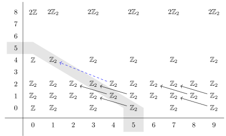
Figure 21: $E_{2}$ page of the AHSS for $\Omega^{\mathrm{Spin}}_{*}(B\mathbb{Z}_{2})$. We show the non-vanishing differentials $d_{2}$ in solid black, and a $d_{3}$ in dashed blue that should vanish in order to reproduce the results of the Smith isomorphism (218).

The second page of the AHSS resulting from this is shown in figure 21. We see that there are many potentially differentials, and many extension problems to be solved, so we will not solve the issue completely. Nevertheless, some useful information can be teased out of the spectral sequence. Clearly, $\Omega_{0}^{\mathrm{Spin}}(B\mathbb{Z}_{2})=\mathbb{Z}$ and $\Omega_{1}^{\mathrm{Spin}}(B\mathbb{Z}_{2})=\mathbb{Z}_{2}\oplus\mathbb{Z}_{2}$, simply because there are no differentials that could enter act on the corresponding entries of the spectral sequence. (In the second identity we have used the splitting result (200).)

Going beyond this requires computing some differentials, using the technology discussed in section 2.2.3. We have that, as a ring, $H^{*}(B\mathbb{Z}_{2},\mathbb{Z}_{2})$ is freely generated by $w_{1}$, the generator of $H^{1}(B\mathbb{Z}_{2},\mathbb{Z}_{2})$:

$$H^{*}(B\mathbb{Z}_{2},\mathbb{Z}_{2})=H^{*}(\mathbb{R}\mathbb{P}^{\infty},\mathbb{Z}_{2})=\mathbb{Z}_{2}[w_{1}]\,.$$ (215)

Using the properties (30) it is then simple to show the relations

$$\mathrm{Sq}^{1}(w^{n})=w\mathrm{Sq}^{1}(w^{n-1})+w^{n+1}\quad;\quad\mathrm{Sq}^{2}(w^{n})=w^{2}\mathrm{Sq}^{1}(w^{n-1})+w\mathrm{Sq}^{2}(w^{n-1})\,.$$ (216)

Using $\mathrm{Sq}^{1}(w)=w^{2}$ and $\mathrm{Sq}^{2}(w)=0$, these are solved by

$$\mathrm{Sq}^{1}(w^{n})=nw^{n+1}\quad\text{and}\quad\mathrm{Sq}^{2}(w^{n})=\frac{n(n-1)}{2}w^{n+2}\,,$$ (217)

with coefficients understood modulo 2. The result is that the differentials which are non-vanishing on the second page are those shown in figure 21, where we have used in addition that the reduction modulo two map $\rho\colon H_{2k+1}(B\mathbb{Z}_{2},\mathbb{Z})\to H_{2k+1}(B\mathbb{Z}_{2},\mathbb{Z}_{2})$ is surjective, which follows easily from $H_{2k}(B\mathbb{Z}_{2},\mathbb{Z})=0$ and exactness of (31).

It is not straightforward to make much further progress using the Atiyah-Hirzebruch spectral sequence, but luckily there is a Smith isomorphism that comes to the rescue here Kapustin:2014dxa :

$$\Omega^{\mathrm{Spin}}_{d}(B\mathbb{Z}_{2})\cong\Omega_{d-1}^{\mathrm{Pin}^{-}}(\mathrm{pt})\oplus\Omega^{\mathrm{Spin}}_{d}(\mathrm{pt})\,.$$ (218)

Using this isomorphism one finds

$$\begin{array}[]{c|ccccccccc}d&0&1&2&3&4&5&6&7&8\\ \hline\cr\Omega^{\mathrm{Spin}}_{d}(B\mathbb{Z}_{2})&\mathbb{Z}&2\mathbb{Z}_{2}&2\mathbb{Z}_{2}&\mathbb{Z}_{8}&\mathbb{Z}&0&0&\mathbb{Z}_{16}&2\mathbb{Z}\end{array}$$ (219)

which can be easily checked to be compatible with the structure of the exact sequence above.

C.4 $\mathrm{Spin}^{\mathbb{Z}_{4}}$ bordism in four dimensions

As discussed in TeichnerPhD ; Teichner , the Atiyah-Hirzebruch spectral sequence for $\Omega^{\mathrm{Spin}^{\mathbb{Z}_{4}}}$ agrees on the first page with the one for $\Omega_{*}^{\mathrm{Spin}}(B\mathbb{Z}_{2})$ we have just computed, but the differentials are different, being twisted.

Figure 22: $E_{2}$ page of the AHSS for $\Omega^{\mathrm{Spin}^{\mathbb{Z}_{4}}}(\mathrm{pt})$. We have shaded the entries relevant for the computation of four dimensional $\theta$ angles.

Clearly the $E_{2}^{(0,4)}=\mathbb{Z}$ entry survives to $E_{\infty}$. We would now like to argue that $E_{2}^{(2,2)}$ does too. To see this, notice that it can only be killed either by being the target of a differential coming from a term of total degree 5. But no such differential can exist, since otherwise $|\Omega_{5}^{\mathrm{Spin}^{\mathbb{Z}_{4}}}|<16$, and this was proven not to be the case in Tachikawa:2018njr . On the other hand, the differential $d_{2}^{w}\colon E_{2}^{(3,1)}\to E_{2}^{(1,2)}$ is non-vanishing. This is because $d_{2}^{w}$ is the dual of $\mathrm{Sq}^{2}_{w}$ TeichnerPhD ; Teichner , defined as $\mathrm{Sq}^{2}_{w}(x)=\mathrm{Sq}^{2}(x)+w^{2}\smile x$, with $w^{2}$ the generator of $H^{2}(B\mathbb{Z}_{2},\mathbb{Z}_{2})$. We $\mathrm{Sq}^{2}w=0$, so $\mathrm{Sq}^{2}_{w}(w)=w^{3}\neq 0$.

We then find that

$$0\to\mathbb{Z}\to\Omega^{\mathrm{Spin}^{\mathbb{Z}_{4}}}_{4}(\mathrm{pt})\to\mathbb{Z}_{2}\to 0$$ (220)

is exact. The physical interpretation of this computation depends on whether this extension is trivial or not. If it is trivial, and $\Omega^{\mathrm{Spin}^{\mathbb{Z}_{4}}}_{4}(\mathrm{pt})=\mathbb{Z}\oplus\mathbb{Z}_{2}$, this would give a candidate for the K-theoretical $\theta$ angles discussed in 5. If the extension is non-trivial, so that $\Omega^{\mathrm{Spin}^{\mathbb{Z}_{4}}}_{4}(\mathrm{pt})=\mathbb{Z}$, we would instead have that there are some $\mathrm{Spin}^{\mathbb{Z}_{4}}$ manifolds which have $\int\!\hat{A}=\frac{1}{24}p_{1}=1$. (Recall that for four dimensional $\mathrm{Spin}$ manifolds one has $\int\!\hat{A}\in 2\mathbb{Z}$.)

Either way, an example of a four-dimensional space that is not $\mathrm{Spin}$ but it is $\mathrm{Spin}^{\mathbb{Z}_{4}}$ is given by the Enriques surface $\mathscr{E}=\text{K3}/\sigma$ (see barth2015compact for a review), where $\sigma$ is a fixed-point-free $\mathbb{Z}_{2}$ action on K3. This surface is not $\mathrm{Spin}$: its signature is 8, while Rochlin’s theorem states that the signature is always a multiple of 16 on four-dimensional $\mathrm{Spin}$ manifolds. Nevertheless, it admits a $\mathrm{Spin}^{\mathbb{Z}_{4}}$ structure: consider the Voisin-Borcea (Calabi-Yau, and thus $\mathrm{Spin}$) manifold $X=(\text{K3}\times T^{2})/\hat{\sigma}$, where $\hat{\sigma}$ acts as $\sigma$ on K3, and as reflection along both coordinates of the $T^{2}$. This space can be understood as a $T^{2}$ fibration with base $\mathscr{E}$. If we consider spinors on $X$, and reduce along the $T^{2}$, we obtain a natural $\mathrm{Spin}^{\mathbb{Z}_{4}}$ structure on $\mathscr{E}$ (since reflections square to $(-1)^{F}$, on fermions they act as a $\mathbb{Z}_{4}$).

We can now discard the possibility of a trivial extension by the following argument. Assume that the sequence (220) does split. We then have that K3 is a generator of $\Omega_{d}^{\mathrm{Spin}^{\mathbb{Z}_{4}}}=\mathbb{Z}\oplus\mathbb{Z}_{2}$. The other generator is some space $X$ which is not $\mathrm{Spin}$, and such that $2X\sim 0$ in $\mathrm{Spin}^{\mathbb{Z}_{4}}$ bordism. Since we showed above that $\mathscr{E}$ is $\mathrm{Spin}^{\mathbb{Z}_{4}}$, it should be the case that $2\mathscr{E}\sim 0$ in $\Omega_{4}^{\mathrm{Spin}^{\mathbb{Z}_{4}}}$. But this is not the case: the embedding $\mathbb{Z}_{4}\to U(1)$ induces an homomorphism $(\mathrm{Spin}(d)\times\mathbb{Z}_{4})/\mathbb{Z}_{2}\to(\mathrm{Spin}(d)\times U(1))/\mathbb{Z}_{2}$ which in turn induces a natural homomorphism

$$\sigma\colon\Omega_{d}^{\mathrm{Spin}^{\mathbb{Z}_{4}}}\to\Omega_{d}^{\mathrm{Spin}^{c}}\,.$$ (221)

So $2\mathscr{E}\sim 0$ in $\Omega_{4}^{\mathrm{Spin}^{\mathbb{Z}_{4}}}$ would induce the relation $2\mathscr{E}\sim 0$ in $\mathrm{Spin}^{c}$. A manifold is trivial in $\mathrm{Spin}^{c}$ iff all its Pontryagin and Stiefel-Whitney characteristic numbers vanish (see theorem 3.1.1 of GilkeyBook ), but we have $p_{1}(\mathscr{E})=24$, so $p_{1}(2\mathscr{E})=2p_{1}(\mathscr{E})=48$, and we arrive to a contradiction.

Finally, let us list some low degree groups that are easily computable from the Atiyah-Hirzebruch spectral sequence:

$$\begin{array}[]{c|ccccccc}d&0&1&2&3&4&5&6\\ \hline\cr\Omega^{\mathrm{Spin}^{\mathbb{Z}_{4}}}_{d}(\mathrm{pt})&\mathbb{Z}&e(\mathbb{Z}_{2},\mathbb{Z}_{2})&0&0&\mathbb{Z}&\mathbb{Z}_{16}&0\end{array}$$ (222)

Appendix D 3d currents

Suppose we have two 3d fermions $\lambda_{1},\lambda_{2}$, with Lagrangian

$$\lambda_{1}^{T}\epsilon\not{\partial}\lambda_{1}+\lambda_{2}^{T}\epsilon\not{\partial}\lambda_{2}.$$ (223)

This system has a $U(1)$ symmetry

$$\left(\begin{array}[]{c}\lambda_{1}\\ \lambda_{2}\end{array}\right)\rightarrow\left(\begin{array}[]{cc}\cos\theta&-\sin\theta\\ \sin\theta&\cos\theta\end{array}\right)\left(\begin{array}[]{c}\lambda_{1}\\ \lambda_{2}\end{array}\right).$$ (230)

which is associated via Noether’s theorem to the current

$$J^{\mu}=\lambda_{1}^{T}\epsilon\gamma^{\mu}\lambda_{2}.$$ (231)

Mass terms can be constructed with the invariant $\epsilon$ tensor. There is just one possibility compatible with the $U(1)$ symmetry, namely

$$\lambda_{1}^{T}\epsilon\lambda_{1}+\lambda_{2}^{T}\epsilon\lambda_{2}.$$ (232)

We can also consider a $R$ or $CR$ discrete symmetry, which we will call $\mathcal{S}$, which acts on the fermions with a phase:

$$\mathcal{S}_{\alpha}\lambda_{1}=\lambda_{1},\quad\mathcal{S}_{\alpha}\lambda_{2}=\alpha\lambda_{2}.$$ (233)

The sign $\alpha$ in the second term can be mapped to whether or not $\mathcal{S}$ commutes or anticommutes with the generator of $U(1)$ rotations. If $\alpha=-1$, it anticommutes: when continuing $\mathcal{S}_{\alpha}$ to Minkowskian signature, it will become a $T$ transformation which commutes with the electric charge, as is usually the case. If $\alpha=+1$, it commutes, which corresponds after analytic continuation to a twisted gauge field which transforms under parity reversal as an ordinary 1-form.

Both possibilities are acceptable, and they both lead to symmetry protected topological phases, but the mechanism in each case is different:

• If $\alpha=+1$, then parity forbids not only the mass term (232), but also the only additional possibility

  $$\lambda_{1}^{T}\epsilon\lambda_{2}.$$ (234)

  Thus, these fermions are protected by virtue of $\mathcal{S}_{\alpha}$-symmetry alone; the fact that they are also charged under a $U(1)$ is irrelevant to the question of existence of protected massless modes. The system is actually the $\nu=2$ topological superconductor Witten:2015aba ; from this discussion we have only learnt that it can be consistently coupled to a twisted gauge field. Since gauge transformations commute with inversions, this is a $\mathrm{Pin}^{c}$ structure.

• If $\alpha=-1$, then $\mathcal{S}_{\alpha}$-symmetry would allow for a mass term (234), so it is not enough to protect the existence of massless modes. However, this mass term is in turn forbidden by the $U(1)$ symmetry, so that the massless fermions are indeed protected: this is the standard topological insulator Witten:2015aba .

This state of affairs is summarized in table 5.

Symmetry	$\lambda_{i}^{T}\epsilon\lambda_{i}$	$\lambda_{i}^{T}\epsilon\lambda_{j}$
$\mathcal{S}_{-1}$	✗	✗
$\mathcal{S}_{+1}$	✗	✓
$Q$	✓	✗

Table 5: Different symmetry generators and the mass terms they allow. $\mathcal{S}_{+1}$ is enough to forbid all mass terms - this is the symmetry of the topological superconductor. The combination of $Q$ and $\mathcal{S}_{-1}$ are also enough to forbid all mass terms - this is the symmetry of the topological insulator. Neither $Q$ or $\mathcal{S}_{+1}$ on their own are able to ensure the existence of a massless fermion.

Appendix E Alternate generators for $\Omega_{5}^{\mathrm{Spin}}(B\mathbb{Z}_{n})$

Here, we present an alternate set of generators for $\Omega_{5}^{\mathrm{Spin}}(B\mathbb{Z}_{n})$, different to the one used in section 4.1. To do this, we have to generalize the notion of a lens space. Pick a vector $\vec{q}=(q_{1},q_{2},\ldots,q_{l})$, where all the entries are coprime. Then we define the generalized lens space $L(n;\vec{q})$ as the quotient of the unit sphere $S^{2l-1}\subset\mathbb{C}^{l}$ by the equivalence relation

$$(z_{1},\ldots,z_{l})\,\equiv\,(z_{1}e^{\frac{2\pi iq_{1}}{n}},\ldots,z_{l}e^{\frac{2\pi iq_{l}}{n}}).$$ (235)

With this notation, we have $L^{l}(n)=L(n;1,1\ldots)$. There is a general expression GilkeyBook for the $\eta$ invariant

$$\eta(L^{l}(n;\vec{q}),s)=-\frac{d}{n}\text{Td}_{l}(n,q_{1},\ldots q_{l};s-l(q_{1}+\ldots+q_{l}),$$ (236)

where $\text{Td}_{l}$ is a specific linear combination of Todd polynomials (we refer the reader to GilkeyBook for details), and $d$ is an integer that must satisfy $dq_{1}\ldots q_{l}\equiv 0\,\text{mod}\,24n$.

Reference GilkeyBook also shows that the bordism group $\Omega_{5}^{\mathrm{Spin}}(B\mathbb{Z}_{n})$ is generated by $L(n;1,1,1)$ and $L(n;1,1,2)$. The $L(n;1,1,1)$ case is straightforward and worked out in the main text.

The $L(n;1,1,2)$ case is more involved. This is because $\gcd(2,24n)\neq 1$, so we cannot straightforwardly apply theorem 4.5.4 of GilkeyBook . Nevertheless, it is clear from the definitions above that $L(n;1,1,2)=L(n;1,1,2+3n)$, and it is easy show that $\gcd(2+3n,24n)=1$ for $n$ odd. So the conditions of the theorem apply to this presentation of the space. A somewhat tricky point now comes from $d$, which is defined to be the inverse of $(2+3n)$ modulo $24n$. We would like to find a polynomial expression for $d$ such that

$$d(2+3n)\equiv 1\mod 24n\,.$$ (237)

From Euler’s theorem:

$$d\equiv(2+3n)^{-1}\equiv(2+3n)^{\phi(24n)-1}\mod 24n$$ (238)

where $\phi(x)$ is Euler’s totient function (counting the number of positive integers smaller or equal to $x$ that are relatively prime to $x$). Expanding, we have

$$(2+3n)^{\phi(24n)-1}=\sum_{p=0}^{\phi(24n)-1}\begin{pmatrix}\phi(24n)-1\\ p\end{pmatrix}2^{p}(3n)^{\phi(24n)-1-p}\,.$$ (239)

Since we work modulo $24n=2^{3}\cdot 3n$ we can drop the terms in the sum with $\phi(24n)-2\geq p\geq 3$, and we find

$$\begin{split}(2+3n)^{\phi(24n)-1}&\equiv(3n)^{\phi(24n)-1}+(\phi(24n)-1)2(3n)^{\phi(24n)-2}\\ &+\frac{1}{2}(\phi(24n)-1)(\phi(24n)-2)2^{2}(3n)^{\phi(24n)-3}+2^{(\phi(24n)-1)}\mod 24n\,.\end{split}$$ (240)

Using $\phi(24n)=\phi(8)\phi(3n)=4\phi(3n)$, this simplifies to:

$$(2+3n)^{4\phi(3n)-1}\equiv(3n)^{4\phi(3n)-1}-2(3n)^{4\phi(3n)-2}+4(3n)^{4\phi(3n)-3}+2^{(4\phi(3n)-1)}\mod 24n\,.$$ (241)

We can simplify this further using that:

$$(3n)^{4\phi(3n)-1} \equiv 3n\mod 24n\,,$$ (242a)

$$(3n)^{4\phi(3n)-2} \equiv 9n^{2}\mod 12n\,,$$ (242b)

$$(3n)^{4\phi(3n)-3} \equiv 3n\mod 6n\,.$$ (242c)

These relations can be proven as follows. Consider for instance (242a). Since $4\phi(3n)-1>0$ for the cases of interest, both sides include a common factor of $3n$. So (242a) is equivalent to

$$(3n)^{4\phi(3n)-2}\equiv 1\mod 8\,.$$ (243)

We have $\gcd(8,3n)=1$ and $\phi(8)=4$, so $(3n)^{4}=1$ mod 8, which implies

$$(3n)^{4\phi(3n)-2}\equiv(3n)^{2}\mod 8\,.$$ (244)

Subtracting both equations, we get

$$(3n)^{2}-1\equiv(3n+1)(3n-1)\equiv 0\mod 8\,.$$ (245)

This follows since we are multiplying two consecutive even numbers, which necessarily gives a multiple of 8. The two other relations can be proven similarly: (242c) follows from $3n^{k}\equiv 1$ mod 2 for all $k>0$ (since $3n$ is odd), while (242b) follows from

$$(3n)^{4\phi(3n)-3}\equiv 3n\mod 4\,.$$ (246)

Using these relations, we find that

$$(2+3n)^{4\phi(3n)-1}\equiv 3n(5-6n)+2^{(4\phi(3n)-1)}\mod 24n\,.$$ (247)

We can in fact do better. From Euler’s theorem we have that

$$(2+3n)^{4\phi(3n)-1}(2+3n)\equiv\bigl{[}3n(5-6n)+2^{(4\phi(3n)-1)}\bigr{]}(2+3n)\equiv 1\mod 24n\,.$$ (248)

Expanding, this leads to

$$2\cdot 2^{(4\phi(3n)-1)}\equiv 1-(3n)^{2}\mod 24n\,.$$ (249)

As explained above, $(3n)^{2}-1$ is a multiple of 8, so we can try dividing both sides by 2 to get a stronger result. Since $\gcd(2,24n)\neq 1$ we should not expect that dividing by two gives a correct result. And indeed, after some trial and error we obtain an ansatz (which we will prove to be correct momentarily) with a correction term:

$$\begin{split}2^{(4\phi(3n)-1)}&\equiv\frac{1}{2}(1-3n^{2})+\frac{1}{2}(3n)(3n^{2}-8n+13)\\ &\equiv\frac{1}{2}\cdot(9n^{3}-33n^{2}+39n+1)\mod 24n\end{split}$$ (250)

for all odd $n$. Our final result is then that

$$d\equiv(2+3n)^{-1}\equiv\frac{1}{2}(9n^{3}-69n^{2}+69n+1)\mod 24n\,.$$ (251)

It is easy to check that $d(2+3n)\equiv 1$ mod $24n$ for $n$ odd holds, as required.

Using this expression we obtain (again after some simplifications)

$$\eta(L(n;1,1,2),s)\equiv\frac{1}{24n}\left((6n^{2}-2)s^{3}-(7n^{2}-3)s\right)\mod 1\,.$$ (252)

Summarizing, so far we find that a $\mathbb{Z}_{n}$ symmetry, with $n$ odd, is anomaly-free if and only if both

$$\sum_{i}\left[4s_{i}^{3}-(n^{2}+3)s_{i}\right]\equiv 0\mod 24n$$ (253)

and (252) vanish modulo integers, when summed over all fermions:

$$\sum_{i}\left[4s_{i}^{3}-(n^{2}+3)s_{i}\right]\equiv\sum_{i}\left[(6n^{2}-2)s_{i}^{3}-(7n^{2}-3)s_{i}\right]\equiv 0\mod 24n\,.$$ (254)

These equations can be simplified: expressing them in terms of $k=(n+1)/2$, and removing an overall factor, they become:

$$\sum_{i}\left[s_{i}^{3}-(k^{2}-k+1)s_{i}\right] \equiv 0\mod 6(2k-1)$$ (255a)

$$\sum_{i}\left[(6k^{2}-6k+1)s_{i}^{3}-(7k^{2}-7k+1)s_{i}\right] \equiv 0\mod 6(2k-1)\,.$$ (255b)

Subtracting $(6k^{2}-6k+1)$ times the first equation from the second we are led to:

$$k^{2}(k-1)^{2}\sum_{i}s_{i}\equiv 0\mod(2k-1)\,.$$ (256)

Since $\gcd(k^{2}(k-1)^{2},2k-1)=1$, we can invert the coefficient, and we obtain the equivalent equation

$$\sum_{i}s_{i}\equiv 0\mod(2k-1)\,.$$ (257)

So we have simplified (255) to

$$\sum_{i}\left[s_{i}^{3}-(k^{2}-k+1)s_{i}\right] \equiv 0\mod 6(2k-1)$$ (258a)

$$\sum_{i}s_{i} \equiv 0\mod(2k-1)\,.$$ (258b)

or equivalently in terms of $n$

$$\sum_{i}\left[s_{i}^{3}-\frac{1}{4}(n^{2}+3)s_{i}\right] \equiv 0\mod 6n$$ (259a)

$$\sum_{i}s_{i} \equiv 0\mod n\,.$$ (259b)

which are precisely (113b).

References

- (1) G. ’t Hooft, C. Itzykson, A. Jaffe, H. Lehmann, P. K. Mitter, I. M. Singer et al., Recent Developments in Gauge Theories. Proceedings, Nato Advanced Study Institute, Cargese, France, August 26 - September 8, 1979, NATO Sci. Ser. B 59 (1980) pp.1–438.
- (2) E. Witten, An SU(2) Anomaly, Phys. Lett. 117B (1982) 324–328.
- (3) A. Kapustin, R. Thorngren, A. Turzillo and Z. Wang, Fermionic Symmetry Protected Topological Phases and Cobordisms, JHEP 12 (2015) 052, [1406.7329].
- (4) C.-T. Hsieh, G. Y. Cho and S. Ryu, Global anomalies on the surface of fermionic symmetry-protected topological phases in (3+1) dimensions, Phys. Rev. B93 (2016) 075135, [1503.01411].
- (5) E. Witten, Fermion Path Integrals And Topological Phases, Rev. Mod. Phys. 88 (2016) 035001, [1508.04715].
- (6) D. S. Freed, Pions and Generalized Cohomology, J. Diff. Geom. 80 (2008) 45–77, [hep-th/0607134].
- (7) C.-T. Hsieh, Discrete gauge anomalies revisited, 1808.02881.
- (8) E. Witten, GLOBAL GRAVITATIONAL ANOMALIES, Commun. Math. Phys. 100 (1985) 197.
- (9) L. Alvarez-Gaume, S. Della Pietra and G. W. Moore, Anomalies and Odd Dimensions, Annals Phys. 163 (1985) 288.
- (10) A. Bilal, Lectures on Anomalies, 0802.0634.
- (11) A. Hatcher, Algebraic topology. Cambridge Univ. Press, Cambridge, 2000.
- (12) D. S. Freed, Determinants, Torsion, and Strings, Commun. Math. Phys. 107 (1986) 483–513.
- (13) I. García-Etxebarria, H. Hayashi, K. Ohmori, Y. Tachikawa and K. Yonekura, 8d gauge anomalies and the topological Green-Schwarz mechanism, JHEP 11 (2017) 177, [1710.04218].
- (14) L. Alvarez-Gaume and P. H. Ginsparg, The Topological Meaning of Nonabelian Anomalies, Nucl. Phys. B243 (1984) 449–474.
- (15) K. Yonekura, Dai-Freed theorem and topological phases of matter, JHEP 09 (2016) 022, [1607.01873].
- (16) M. F. Atiyah and I. M. Singer, The Index of elliptic operators. 1, Annals Math. 87 (1968) 484–530.
- (17) X.-z. Dai and D. S. Freed, eta invariants and determinant lines, J. Math. Phys. 35 (1994) 5155–5194, [hep-th/9405012].
- (18) M. F. Atiyah, V. K. Patodi and I. M. Singer, Spectral asymmetry and Riemannian Geometry 1, Math. Proc. Cambridge Phil. Soc. 77 (1975) 43.
- (19) M. F. Atiyah, V. K. Patodi and I. M. Singer, Spectral asymmetry and Riemannian geometry II, Math. Proc. Cambridge Phil. Soc. 78 (1976) 405.
- (20) M. F. Atiyah, V. K. Patodi and I. M. Singer, Spectral asymmetry and Riemannian geometry. III, Mathematical Proceedings of the Cambridge Philosophical Society 79 (1976) 71–99.
- (21) S. Monnier, The global anomalies of (2,0) superconformal field theories in six dimensions, JHEP 09 (2014) 088, [1406.4540].
- (22) S. B. Giddings and A. Strominger, Axion Induced Topology Change in Quantum Gravity and String Theory, Nucl. Phys. B306 (1988) 890–907.
- (23) E. Witten, Anti-de Sitter space, thermal phase transition, and confinement in gauge theories, Adv. Theor. Math. Phys. 2 (1998) 505–532, [hep-th/9803131].
- (24) D. S. Freed, Anomalies and Invertible Field Theories, Proc. Symp. Pure Math. 88 (2014) 25–46, [1404.7224].
- (25) S. Monnier, A Modern Point of View on Anomalies, in Durham Symposium, Higher Structures in M-Theory Durham, UK, August 12-18, 2018, 2019. 1903.02828.
- (26) F. Benini, C. Córdova and P.-S. Hsin, On 2-Group Global Symmetries and their Anomalies, 1803.09336.
- (27) L. Nicolaescu, Notes on Seiberg-Witten Theory. Graduate studies in mathematics. American Mathematical Society, 2000.
- (28) M. Guo, P. Putrov and J. Wang, Time reversal, SU(N) Yang–Mills and cobordisms: Interacting topological superconductors/insulators and quantum spin liquids in 3+1D, Annals Phys. 394 (2018) 244–293, [1711.11587].
- (29) J. Wang, K. Ohmori, P. Putrov, Y. Zheng, Z. Wan, M. Guo et al., Tunneling Topological Vacua via Extended Operators: (Spin-)TQFT Spectra and Boundary Deconfinement in Various Dimensions, PTEP 2018 (2018) 053A01, [1801.05416].
- (30) J. McCleary, A User’s Guide to Spectral Sequences. Cambridge Studies in Advanced Mathematics. Cambridge University Press, 2 ed., 2000. 10.1017/CBO9780511626289.
- (31) J. Davis and P. Kirk, Lecture Notes in Algebraic Topology. Graduate studies in mathematics. American Mathematical Society, 2001.
- (32) D. W. Anderson, E. H. Brown and F. P. Peterson, Spin cobordism, Bull. Amer. Math. Soc. 72 (03, 1966) 256–260.
- (33) R. Stong, Calculation of , in Unified String Theories (M. Green and D. Gross, eds.), World Scientific, 1986.
- (34) P. Teichner, Topological four-manifolds with finite fundamental group. PhD thesis, Johannes-Gutenberg Universität in Mainz, 1992.
- (35) P. Teichner, On the signature of four-manifolds with universal covering spin, Mathematische Annalen (1993) 745–759.
- (36) J. Adams and J. Adams, Stable Homotopy and Generalised Homology. Chicago Lectures in Mathematics. University of Chicago Press, 1995.
- (37) W.-T. Wu, Les i-carrés dans une variété grassmannienne, pp. 19–21. World Scientific, 2012.
- (38) A. Borel, La cohomologie mod 2 de certains espaces homogènes., Commentarii mathematici Helvetici 27 (1953) 165–197.
- (39) E. Milnor, J. Milnor, J. Stasheff, J. Mather and P. Griffiths, Characteristic Classes. Annals of mathematics studies. Princeton University Press, 1974.
- (40) J. H. Fung, “The Cohomology of Lie groups.” http://math.uchicago.edu/~may/REU2012/REUPapers/Fung.pdf.
- (41) K. Marathe, Topics in Physical Mathematics: Geometric Topology and Field Theory. Springer, 2010. 10.1007/978-1-84882-939-8.
- (42) R. Switzer, Algebraic Topology: Homotopy and Homology. Classics in Mathematics. Springer, 2002.
- (43) K. A. Intriligator, D. R. Morrison and N. Seiberg, Five-dimensional supersymmetric gauge theories and degenerations of Calabi-Yau spaces, Nucl. Phys. B497 (1997) 56–100, [hep-th/9702198].
- (44) A. N. Redlich, Gauge Noninvariance and Parity Violation of Three-Dimensional Fermions, Phys. Rev. Lett. 52 (1984) 18.
- (45) A. N. Redlich, Parity Violation and Gauge Noninvariance of the Effective Gauge Field Action in Three-Dimensions, Phys. Rev. D29 (1984) 2366–2374.
- (46) D. Husemöller, M. Joachim, B. Jurco and M. Schottenloher, Basic Bundle Theory and K-Cohomology Invariants. Lecture Notes in Physics. Springer Berlin Heidelberg, 2007.
- (47) D.-E. Diaconescu, G. W. Moore and E. Witten, E(8) gauge theory, and a derivation of K theory from M theory, Adv. Theor. Math. Phys. 6 (2003) 1031–1134, [hep-th/0005090].
- (48) A. Bahri and P. Gilkey, The eta invariant, bordism, and equivariant bordism for cyclic -groups., Pacific J. Math. 128 (1987) 1–24.
- (49) E. Witten, Topological Tools in Ten-dimensional Physics, Int. J. Mod. Phys. A1 (1986) 39.
- (50) D. Fuchs and O. Viro, Topology II: Homotopy and Homology. Classical Manifolds. Encyclopaedia of Mathematical Sciences. Springer Berlin Heidelberg, 2003.
- (51) A. Borel, Topology of lie groups and characteristic classes, Bull. Amer. Math. Soc. 61 (09, 1955) 397–432.
- (52) A. Borel and J.-P. Serre, Groupes de lie et puissances reduites de steenrod, American Journal of Mathematics 75 (1953) 409–448.
- (53) D. Tong, Line Operators in the Standard Model, JHEP 07 (2017) 104, [1705.01853].
- (54) S. Monnier, G. W. Moore and D. S. Park, Quantization of anomaly coefficients in 6D supergravity, JHEP 02 (2018) 020, [1711.04777].
- (55) K.-w. Choi, D. B. Kaplan and A. E. Nelson, Is CP a gauge symmetry?, Nucl. Phys. B391 (1993) 515–530, [hep-ph/9205202].
- (56) P. Gilkey, The Geometry of Spherical Space Form Groups. Series in pure mathematics. World Scientific, 1989.
- (57) M. Berg, C. De Witt-Morette, S. Gwo and E. Kramer, The Pin Groups in Physics, Reviews in Mathematical Physics 13 (2001) 953–1034, [math-ph/0012006].
- (58) Y. Tachikawa and K. Yonekura, Why are fractional charges of orientifolds compatible with Dirac quantization?, 1805.02772.
- (59) X. Gu, On the Cohomology of the Classifying Spaces of Projective Unitary Groups, ArXiv e-prints (Dec., 2016) , [1612.00506].
- (60) J. Rotman, An Introduction to Algebraic Topology. Graduate Texts in Mathematics. Springer New York, 1998.
- (61) L. Breen, R. Mikhailov and A. Touzé, Derived functors of the divided power functors, ArXiv e-prints (Dec., 2013) , [1312.5676].
- (62) H. Cartan, Séminaire Henri Cartan de l’Ecole Normale Supérieure, 1954/1955. Algèbres d’Eilenberg-MacLane et homotopie, .
- (63) N. Pointet-Tischler, La suspension cohomologique des espaces d’eilenberg-maclane, Comptes Rendus de l’Académie des Sciences - Series I - Mathematics 325 (1997) 1113 – 1116.
- (64) N. Tischler, Invariants de Postnikov des espaces de lacets. PhD thesis, Université de Lausanne, 1996.
- (65) A. Clément, Integral Cohomology of Finite Postnikov Towers. PhD thesis, Université de Lausanne, 2002.
- (66) M. Feshbach, The integral cohomology rings of the classifying spaces of o(n) and so(n), Indiana University Mathematics Journal 32 (1983) 511–516.
- (67) E. H. Brown, The Cohomology of and with Integer Coefficients, Proceedings of the American Mathematical Society 85 (1982) 283–288.
- (68) M. FESHBACH, The integral cohomology rings of the classifying spaces of o(n) and so(n), Indiana University Mathematics Journal 32 (1983) 511–516.
- (69) D. QUILLEN, The mod 2 cohomology rings of extra-special 2-groups and the spinor groups., Mathematische Annalen 194 (1971) 197–212.
- (70) A. Kono, On the integral cohomology of , J. Math. Kyoto Univ. 26 (1986) 333–337.
- (71) M. Kameko and M. Mimura, On the Rothenberg-Steenrod spectral sequence for the mod 2 cohomology of classifying spaces of spinor groups, ArXiv e-prints (Apr., 2009) , [0904.0800].
- (72) S. R. Edwards, On the spin bordism of , Illinois J. Math. 35 (12, 1991) 683–689.
- (73) L. E. Ibanez and G. G. Ross, Discrete gauge symmetry anomalies, Phys. Lett. B260 (1991) 291–295.
- (74) L. E. Ibanez, More about discrete gauge anomalies, Nucl. Phys. B398 (1993) 301–318, [hep-ph/9210211].
- (75) H. K. Dreiner, C. Luhn and M. Thormeier, What is the discrete gauge symmetry of the MSSM?, Phys. Rev. D73 (2006) 075007, [hep-ph/0512163].
- (76) R. N. Mohapatra and M. Ratz, Gauged Discrete Symmetries and Proton Stability, Phys. Rev. D76 (2007) 095003, [0707.4070].
- (77) H. M. Lee, S. Raby, M. Ratz, G. G. Ross, R. Schieren, K. Schmidt-Hoberg et al., Discrete R symmetries for the MSSM and its singlet extensions, Nucl. Phys. B850 (2011) 1–30, [1102.3595].
- (78) H. P. Nilles, M. Ratz and P. K. S. Vaudrevange, Origin of Family Symmetries, Fortsch. Phys. 61 (2013) 493–506, [1204.2206].
- (79) M.-C. Chen, M. Fallbacher, M. Ratz, A. Trautner and P. K. S. Vaudrevange, Anomaly-safe discrete groups, Phys. Lett. B747 (2015) 22–26, [1504.03470].
- (80) P. B. Gilkey and B. Botvinnik, The eta invariant and the equivariant spin bordism of spherical space form 2 groups, pp. 213–223. Springer Netherlands, Dordrecht, 1996.
- (81) P. B. Gilkey, The eta invariant of pin manifolds with cyclic fundamental groups, Periodica Mathematica Hungarica 36 (Apr, 1998) 139–170.
- (82) L. E. Ibanez and G. G. Ross, Discrete gauge symmetries and the origin of baryon and lepton number conservation in supersymmetric versions of the standard model, Nucl. Phys. B368 (1992) 3–37.
- (83) D. Gaiotto, A. Kapustin, Z. Komargodski and N. Seiberg, Theta, Time Reversal, and Temperature, JHEP 05 (2017) 091, [1703.00501].
- (84) D. Gaiotto, Z. Komargodski and N. Seiberg, Time-reversal breaking in QCD4, walls, and dualities in 2 + 1 dimensions, JHEP 01 (2018) 110, [1708.06806].
- (85) J. J. van der Bij, A Cosmotopological relation for a unified field theory, Phys. Rev. D76 (2007) 121702, [0708.4179].
- (86) G. E. Volovik and M. A. Zubkov, Standard Model as the topological material, New J. Phys. 19 (2017) 015009, [1608.07777].
- (87) T. P. Cheng and L. F. Li, GAUGE THEORY OF ELEMENTARY PARTICLE PHYSICS. Oxford, Uk: Clarendon ( 1984) 536 P. ( Oxford Science Publications), 1984.
- (88) Particle Data Group collaboration, C. Patrignani et al., Review of Particle Physics, Chin. Phys. C40 (2016) 100001.
- (89) L. N. Chang and C. Soo, The Standard model with gravity couplings, Phys. Rev. D53 (1996) 5682–5691, [hep-th/9406188].
- (90) C. Csaki, The Minimal supersymmetric standard model (MSSM), Mod. Phys. Lett. A11 (1996) 599, [hep-ph/9606414].
- (91) F. Dillen and L. Verstraelen, Handbook of Differential Geometry, Vol.1. Elsevier Science, 1999.
- (92) T. Banks and M. Dine, Note on discrete gauge anomalies, Phys. Rev. D45 (1992) 1424–1427, [hep-th/9109045].
- (93) M. Berasaluce-González, M. Montero, A. Retolaza and A. M. Uranga, Discrete gauge symmetries from (closed string) tachyon condensation, JHEP 1311 (2013) 144, [1305.6788].
- (94) I. García-Etxebarria, M. Montero and A. M. Uranga, Closed tachyon solitons in type II string theory, 1505.05510.
- (95) S. Hellerman, On the landscape of superstring theory in , hep-th/0405041.
- (96) K. Shiozaki, H. Shapourian and S. Ryu, Many-body topological invariants in fermionic symmetry-protected topological phases, Phys. Rev. B95 (2017) 205139, [1609.05970].
- (97) R. Thom, Some “global” properties of differentiable manifolds, pp. 131–209. WORLD SCIENTIFIC, 2012.
- (98) M.-C. Chen, M. Ratz and A. Trautner, Non-Abelian discrete R symmetries, JHEP 09 (2013) 096, [1306.5112].
- (99) T. Banks and N. Seiberg, Symmetries and Strings in Field Theory and Gravity, Phys. Rev. D83 (2011) 084019, [1011.5120].
- (100) M. Berasaluce-Gonzalez, P. G. Camara, F. Marchesano, D. Regalado and A. M. Uranga, Non-Abelian discrete gauge symmetries in 4d string models, JHEP 09 (2012) 059, [1206.2383].
- (101) J. Polchinski, Monopoles, duality, and string theory, Int. J. Mod. Phys. A19S1 (2004) 145–156, [hep-th/0304042].
- (102) D. Gaiotto, A. Kapustin, N. Seiberg and B. Willett, Generalized Global Symmetries, JHEP 02 (2015) 172, [1412.5148].
- (103) Y. Tachikawa and K. Yonekura, On time-reversal anomaly of 2+1d topological phases, PTEP 2017 (2017) 033B04, [1610.07010].
- (104) E. Witten, Five-brane effective action in M theory, J. Geom. Phys. 22 (1997) 103–133, [hep-th/9610234].
- (105) D. S. Freed and G. W. Moore, Setting the quantum integrand of M-theory, Commun. Math. Phys. 263 (2006) 89–132, [hep-th/0409135].
- (106) A. Hattori, Integral characteristic numbers for weakly almost complex manifolds, Topology 5 (sep, 1966) 259–280.
- (107) R. Stong, Relations among characteristic numbers—I, Topology 4 (1965) 267 – 281.
- (108) M. J. Hopkins and M. A. Hovey, Spin cobordism determines real K-theory, Mathematische Zeitschrift 210 (Dec, 1992) 181–196.
- (109) O. Bergman, D. Rodríguez-Gómez and G. Zafrir, Discrete and the 5d superconformal index, JHEP 01 (2014) 079, [1310.2150].
- (110) S. Sethi, A New String in Ten Dimensions?, JHEP 09 (2013) 149, [1304.1551].
- (111) A. Dold and H. Whitney, Classification of oriented sphere bundles over a 4-complex, Annals of Mathematics 69 (1959) 667–677.
- (112) L. M. Woodward, The classification of orientable vector bundles over cw-complexes of small dimension, Proceedings of the Royal Society of Edinburgh: Section A Mathematics 92 (1982) 175–179.
- (113) R. C. Kirby and L. R. Taylor, A calculation of bordism groups, Commentarii Mathematici Helvetici 65 (Dec, 1990) 434–447.
- (114) D. W. Anderson, E. H. Brown and F. P. Peterson, Pin cobordism and related topics, Commentarii Mathematici Helvetici 44 (Dec, 1969) 462–468.
- (115) S. P. Novikov, Homotopy properties of Thom complexes, pp. 211–250. World Scientific, 2012.
- (116) W. Barth, K. Hulek, C. Peters and A. van de Ven, Compact Complex Surfaces. Ergebnisse der Mathematik und ihrer Grenzgebiete. 3. Folge / A Series of Modern Surveys in Mathematics. Springer Berlin Heidelberg, 2015.