Electronic spectral properties of incommensurate twisted trilayer graphene

Abstract

Multilayered van der Waals structures often lack periodicity, which difficults their modeling. Building on previous work for bilayers, we develop a tight-binding based, momentum space formalism capable of describing incommensurate multilayered van der Waals structures for arbitrary lattice mismatch and/or misalignment between different layers. We demonstrate how the developed formalism can be used to model angle-resolved photoemission spectroscopy measurements, and scanning tunnelling spectroscopy which can probe the local and total density of states. The general method is then applied to incommensurate twisted trilayer graphene structures. It is found that the coupling between the three layers can significantly affect the low energy spectral properties, which cannot be simply attributed to the pairwise hybridization between the layers.

I Introduction

The rise of two-dimensional (2D) materials, in recent years, has enabled the study of structures formed by vertically stacked 2D layersPonomarenko et al. (2011); Novoselov and Neto (2012); Geim and Grigorieva (2013). This new kind of structures, generally referred to as van der Waals (vdW) structures due to the interaction that holds the layers together, display new and interesting physics. The properties of vdW structures are determined not only by the properties of the individual layers, but also, sometimes in a fundamental way, by the coupling between different layers, which is affected by the relative lattice mismatch and misalignment.

A prototypical van der Waals structure is twisted bilayer graphene (tBLG). This apparently simple material displays rich and interesting properties that deviate substantially from both single layer and Bernal stacked bilayer graphene. The misalignment between the two layers, which gives origin to moiré patterns, is responsible for the reduction of graphene’s Fermi velocityLopes dos Santos et al. (2007); Yufeng et al. (2010); Luican et al. (2011); Trambly de Laissardière et al. (2010) and to the emergence of low energy van Hove singularitiesLopes dos Santos et al. (2007); Li et al. (2009), both of which are controlled by the twist angle. For very small twist angles, the van Hove singularities that occur above and bellow graphene’s neutrality point can coalesce, leading to the formation of the so called flat bands at the neutrality pointTrambly de Laissardière et al. (2010); Suárez Morell et al. (2010); Bistritzer and MacDonald (2011). Very recently, a strongly correlated Mott insulating phaseCao et al. (2018) and superconductivityCao et al. (line) have been observed in tBLG in the flat band regime. The effect of twist has also been observed in semiconducting transition metal dichalcogenides (STMD). Namelly, it was found that the band gap, and whether it is direct or indirect, of bilayer MoS₂ is controlled by the relative twist angleYeh et al. (2016).

The study of van der Waals structures is not only of fundamental interested, but also has potential technological applications. Hybrid vertical structures formed by graphene/boron nitride/graphene have been shown to display negative differential conductance in their vertical transport characteristics, which can be exploited to create a radio-frequency oscillatorMishchenko et al. (2014). Graphene/boron nitride/grapheneBritnell et al. (2012a, b) and graphene/STMD/graphene structuresBritnell et al. (2012a); Georgiou et al. (2012) were also shown to operate as vertical tunneling field effect transistors with large ON/OFF ratios. Graphene/STMD/graphene structures can also be used as photodetectors with fast response timesBritnell et al. (2013); Yu et al. (2013); Massicotte et al. (2015).

The possible lattice mismatch/misalignment in van der Waals structures and the frequent sensitivity of their properties to those, makes the modelling of such structures challenging. The lattice mismatch/misalignment can give origin to periodic structures with large unit cells, making treatments based on Bloch’s theorem numerically expensive. In the case when the structure is incommensurate, Bloch’s theorem cannot be applied. For the case of tBLG, a momentum space formalism, based on the expansion of the electronic wave function in Bloch states of the individual layers, which can undergo generalized umklapp scattering, has been developedLopes dos Santos et al. (2007); Shallcross et al. (2008); Bistritzer and MacDonald (2010, 2011); Lopes dos Santos et al. (2012); Moon and Koshino (2013); Koshino (2015) (a mathematically formal description of the method can be found in Massatt et al. (2018)). This method has proved to be very useful, allowing to model incommensurate or commensurate, large period structures, at a modest computational cost. This method is not restricted to tBLG, but can be applied to other kinds structures even for large mismatch/misaligment Koshino (2015); Amorim (2018).

Theoretical work up to now has been focused on the study of incommensurate bilayer structures (formed by two lattice mismatched periodic structures). An exception to this is Ref. Correa et al. (2014), where the optical properties of commensurate fully twisted trilayer graphene (tTLG), where all layers are rotated, are studied using ab initio methods. However, the twisted trilayer structures that can be easily simulated is even more restricted than in the bilayer case, due to the even larger unit cells involved. The interest in lattice mismatched/misaligned multilayer structures, such as graphene/boron nitride/graphene and graphene/STMC/graphene, demands the development of numerically efficient methods. The goal of this paper is to extend the momentum space method to multilayer incommensurate structures. We study how the electronic wavefunctions, and the corresponding energies, can be determined and how these can be used to evaluate different measurable spectral quantities, namely, the angle-resolved photoemission spectroscopy (ARPES) intensity, and the total (TDoS) and local densities of states (LDoS), which can be measured via scanning tunnelling spectroscopy (STS). Motivated by recent experimental work Zuo et al. (2018), we use the developed method to study the spectral properties of tTLG.

This paper is organized as follows. The general formalism in developed in Section II. In Section II.1, an effective Hamiltonian in momentum space for incommensurate multilayers is constructed. In Section II.2, it is exemplified how the effective Hamiltonian can be used to model ARPES measurements, LDoS and TDoS. The general formalism is applied to tTLG in Section III. Finally, we conclude in Section IV and also discuss future uses of the formalism.

II Formalism

II.1 Hamiltonian for incommensurate multilayers in momentum space

For simplicity, we will specialize to the case of trilayer structures, which already captures all the conceptual complexity of a multilayer. To clarify, by a trilayer we mean a structure that is formed by three periodic systems which are lattice mismatched/misaligned. In this way, the structure formed by a Bernall-staked graphene bilayer with an additional twisted graphene monolayer, as studied in Ref. Suárez Morell et al. (2013), would be classified as a bilayer. In order to model the electronic properties of incommensurate, lattice mismatched/misaligned multilayer structures, we start from a tight-binding description of the system, as previously done for bilayersLopes dos Santos et al. (2007); Bistritzer and MacDonald (2010); Koshino (2015). The single-electron Hamiltonian of the trilayer reads

$$H=\sum_{\ell=1}^{3}H_{\ell}+\sum_{\ell=1}^{2}\left(H_{\ell+1,\ell}+H_{\ell,\ell+1}\right),$$ (1)

where $H_{\ell}$ ($\ell=1,...,3$) describe the isolated layers, which are assumed to be periodic, and $H_{\ell,\ell^{\prime}}$ describe the hopping of electrons from layer $\ell^{\prime}$ to layer $\ell$, with $H_{\ell^{\prime},\ell}=H_{\ell,\ell^{\prime}}^{\dagger}$. Owing to the exponential suppression of the hopping integrals with distance, we have assumed that only consecutive layers are coupled to each other. In terms of creation and annihilation operators, we write the intralayer Hamiltonians as

$$H_{\ell}=\sum_{\mathbf{R}_{\ell}\alpha,\mathbf{R}_{\ell}^{\prime}\alpha^{\prime}}h_{\alpha\alpha^{\prime}}^{\ell\ell}\left(\mathbf{R}_{\ell},\mathbf{R}_{\ell}^{\prime}\right)c_{\ell,\mathbf{R}_{\ell},\alpha}^{\dagger}c_{\ell,\mathbf{R}_{\ell}^{\prime},\alpha^{\prime}},$$ (2)

where $h_{\alpha\alpha^{\prime}}^{\ell\ell}\left(\mathbf{R}_{\ell},\mathbf{R}_{\ell}^{\prime}\right)=h_{\alpha\alpha^{\prime}}^{\ell\ell}\left(\mathbf{R}_{\ell}-\mathbf{R}_{\ell}^{\prime},\mathbf{0}\right)$ are hopping parameters, which are invariant under lattice translations of layer $\ell$, and $c_{\ell,\mathbf{R}_{\ell},\alpha}^{\dagger}$ creates an electron in a Wannier state of orbital/sublattice character $\alpha$, which is centered at the position $\mathbf{R}_{\ell}+\bm{\tau}_{\ell,\alpha}$, with $\mathbf{R}_{\ell}$ a Bravais lattice site of layer $\ell$ and $\bm{\tau}_{\ell,\alpha}$ the position of the Wannier center within the unit cell. We represent the Wannier states as $\left|\ell,\mathbf{R}_{\ell},\alpha\right\rangle$ and $N_{\text{orb}\ell}$ is the number of Wannier orbitals per unit cell of layer $\ell$. The interlayer terms of the Hamiltonian read

$$H_{\ell,\ell^{\prime}}=\sum_{\mathbf{R}_{\ell}\alpha,\mathbf{R}_{\ell}^{\prime}\beta}h_{\alpha\beta}^{\ell\ell^{\prime}}\left(\mathbf{R}_{\ell},\mathbf{R}_{\ell^{\prime}}\right)c_{\ell,\mathbf{R}_{\ell},\alpha}^{\dagger}c_{\ell^{\prime},\mathbf{R}_{\ell^{\prime}},\beta},$$ (3)

where $h_{\alpha\beta}^{\ell\ell^{\prime}}\left(\mathbf{R}_{\ell},\mathbf{R}_{\ell^{\prime}}\right)$ are interlayer hopping terms, with $\mathbf{R}_{\ell}$($\mathbf{R}_{\ell^{\prime}}$) running over lattice sites of layer $\ell$($\ell^{\prime}$) and $\alpha$($\beta$) running over the orbital/sublattice degrees of freedom of layer $\ell$($\ell^{\prime}$). The Wannier states can be written of Bloch waves, $\left|\ell,\mathbf{k},\alpha\right\rangle$, of the individual layers as

$$\left|\ell,\mathbf{R}_{\ell},\alpha\right\rangle=\frac{1}{\sqrt{N_{\ell}}}\sum_{\mathbf{k}\in\text{BZ}\ell}e^{-i\mathbf{k}\cdot\left(\mathbf{R}_{\ell}+\bm{\tau}_{\ell,\alpha}\right)}\left|\ell,\mathbf{k},\alpha\right\rangle,$$ (4)

where $\text{BZ}\ell$ represents the Brillouin zone for layer $\ell$ and $N_{\ell}$ is the number of unit cells in layer $\ell$. Changing to the Bloch wave basis brings the Hamiltonians of the isolated layers to a block diagonal form

$$H_{\ell}=\sum_{\mathbf{k}\in\text{BZ}\ell,\alpha\alpha^{\prime}}h_{\alpha\alpha^{\prime}}^{\ell\ell}\left(\mathbf{k}\right)c_{\ell,\mathbf{k},\alpha}^{\dagger}c_{\ell,\mathbf{k},\alpha^{\prime}},$$ (5)

where $h_{\alpha\alpha^{\prime}}^{\ell\ell}\left(\mathbf{k}\right)=\sum_{\mathbf{R}_{\ell}}e^{-i\mathbf{k}\cdot\left(\mathbf{R}_{\ell}+\bm{\tau}_{\ell,\alpha}-\bm{\tau}_{\ell,\beta}\right)}h_{\alpha\beta}^{\ell\ell}\left(\mathbf{R}_{\ell},\mathbf{0}\right)$ and $c_{\ell,\mathbf{k},\alpha}^{\dagger}$ creates an electron in the Bloch state $\left|\ell,\mathbf{k},\alpha\right\rangle$. Assuming a two-centre approximation for the interlayer hoppings, these can be written as a Fourier transform Bistritzer and MacDonald (2010); Koshino (2015)

$$h_{\alpha\beta}^{\ell\ell^{\prime}}\left(\mathbf{R}_{\ell},\mathbf{R}_{\ell^{\prime}}\right)=\sqrt{A_{\text{u.c.}\ell}A_{\text{u.c.}\ell^{\prime}}}\times\\ \times\int\frac{d^{2}\mathbf{q}}{\left(2\pi\right)^{2}}e^{i\mathbf{q}\cdot\left(\mathbf{R}_{\ell}+\bm{\tau}_{\ell,\alpha}-\mathbf{R}_{\ell^{\prime}}-\bm{\tau}_{\ell^{\prime},\beta}\right)}h_{\alpha\beta}^{\ell\ell^{\prime}}\left(\mathbf{q}\right),$$ (6)

and the interlayer terms of the Hamiltonian can be written as

$$H_{\ell,\ell^{\prime}}=\sum_{\begin{subarray}{c}\mathbf{k}\in\text{BZ}\ell,\alpha,\mathbf{G}_{\ell}\\ \mathbf{k}^{\prime}\in\text{BZ}\ell^{\prime},\beta,\mathbf{G}_{\ell^{\prime}}\end{subarray}}e^{i\mathbf{G}_{\ell}\cdot\bm{\tau}_{\ell,\alpha}}h_{\alpha\beta}^{\ell\ell^{\prime}}\left(\mathbf{k}+\mathbf{G}_{\ell}\right)e^{-i\mathbf{G}_{\ell^{\prime}}\cdot\bm{\tau}_{\ell^{\prime},\beta}}\\ \times c_{\ell,\mathbf{k},\alpha}^{\dagger}c_{\ell^{\prime},\mathbf{k}^{\prime},\beta}\delta_{\mathbf{k}+\mathbf{G}_{\ell},\mathbf{k}^{\prime}+\mathbf{G}_{\ell^{\prime}}},$$ (7)

where $\mathbf{G}_{\ell}$($\mathbf{G}_{\ell^{\prime}}$) are reciprocal lattice vectors of layer $\ell$($\ell^{\prime}$). The Kronecher symbol in the above equation imposes the generalized umklapp condition Koshino (2015), which states that two Bloch states of layer $\ell$ and $\ell^{\prime}$ with cystal-momentum $\mathbf{k}$ and $\mathbf{k}^{\prime}$, respectively, are only coupled to each other provided reciprocal lattice vectors of layers $\ell$, $\mathbf{G}_{\ell}$ , and $\ell^{\prime}$, $\mathbf{G}_{\ell^{\prime}}$, exist such that $\mathbf{k}+\mathbf{G}_{\ell}=\mathbf{k}^{\prime}+\mathbf{G}_{\ell^{\prime}}$. This condition must be satisfied for each hopping process between two consecutive layers.

Now let us study when two Bloch states of non-consecutive layers, in a multilayer structure, can couple by compounding generalized umklapp processes. Let us consider a trilayer structure. We have a state with momentum $\mathbf{k}_{1}$ of layer $1$, which couples to a state of layer $2$ with momentum $\mathbf{k}_{2}$, provided reciprocal vectors $\mathbf{G}_{1}$ and $\mathbf{G}_{2}$ exist such that $\mathbf{k}_{1}+\mathbf{G}_{1}=\mathbf{k}_{2}+\mathbf{G}_{2}.$ In its turn, state $\mathbf{k}_{2}$ can couple to a state of layer $3$ with momentum $\mathbf{k}_{3}$, provided $\mathbf{G}_{2}^{\prime}$ and $\mathbf{G}_{3}$ exist, such that $\mathbf{k}_{2}+\mathbf{G}_{2}^{\prime}=\mathbf{k}_{3}+\mathbf{G}_{3}.$ Therefore, states $\mathbf{k}_{1}$ and $\mathbf{k}_{3}$ are coupled, provided reciprocal lattice vectors $\mathbf{G}_{1}$ of layer $1$, $\mathbf{G}_{3}$ of layer $3$, $\mathbf{G}_{2}$ and $\mathbf{G}_{2}^{\prime}$ of layer $2$ exist, such that

$$\mathbf{k}_{1}+\mathbf{G}_{1}+\mathbf{G}_{2}^{\prime}=\mathbf{k}_{3}+\mathbf{G}_{3}+\mathbf{G}_{2},$$ (8)

where $\mathbf{G}_{2}$ and $\mathbf{G}_{2}^{\prime}$ can differ. This is immediately satisfied, by working in a extended zone scheme and setting $\mathbf{k}_{1}=\mathbf{p}+\mathbf{G}_{2}+\mathbf{G}_{3}$ and $\mathbf{k}_{3}=\mathbf{p}+\mathbf{G}_{1}+\mathbf{G}_{2}^{\prime}$, with $\mathbf{p}$ defined in the extended reciprocal space. This motivates us to look for eigenstates of Eq. (1) of the form

$$\left|\psi_{\mathbf{k},n}^{\text{umklapp}}\right\rangle=\\ =\sum_{\mathbf{G}_{2},\mathbf{G}_{3},\alpha}\phi_{1,\mathbf{k},\alpha}^{n}\left(\mathbf{G}_{2},\mathbf{G}_{3}\right)\left|1,\mathbf{k}+\mathbf{G}_{2}+\mathbf{G}_{3},\alpha\right\rangle\\ +\sum_{\mathbf{G}_{1},\mathbf{G}_{3},\beta}\phi_{2,\mathbf{k},\beta}^{n}\left(\mathbf{G}_{1},\mathbf{G}_{3}\right)\left|2,\mathbf{k}+\mathbf{G}_{1}+\mathbf{G}_{3},\beta\right\rangle\\ +\sum_{\mathbf{G}_{1},\mathbf{G}_{2},\gamma}\phi_{3,\mathbf{k},\gamma}^{n}\left(\mathbf{G}_{1},\mathbf{G}_{2}\right)\left|3,\mathbf{k}+\mathbf{G}_{1}+\mathbf{G}_{2},\gamma\right\rangle,$$ (9)

which is a superposition of Bloch states of the three layers, where the Bloch state from one layer can undergo generalized umklapp scattering due to the remaining two layers. The generalization for the multilayer case is formally straightforward: the multilayer eigenstates are formed by a superposition of Bloch states of each layer, which can undergo umklapp scattering by reciprocal lattice vectors of all the remaining ones.

By suitably truncating the sums over reciprocal lattice vectors in Eq. (9), we obtain an effective Hamiltonian which can be written as

$$\bm{H}_{\mathbf{k}}^{\text{umklapp}}=\left[\begin{array}[]{ccc}\bm{H}_{\mathbf{k}}^{11}&\bm{H}_{\mathbf{k}}^{12}&\bm{0}\\ \bm{H}_{\mathbf{k}}^{21}&\bm{H}_{\mathbf{k}}^{22}&\bm{H}_{\mathbf{k}}^{23}\\ \bm{0}&\bm{H}_{\mathbf{k}}^{32}&\bm{H}_{\mathbf{k}}^{33}\end{array}\right],$$ (10)

with the matrix entries running over $\mathbf{G}_{2},\mathbf{G}_{3},\alpha$ for the layer $1$ sector, and equivalently for the two other layers. In the above expression, $\bm{H}_{\mathbf{k}}^{11}$ is a block diagonal matrix, with entries given by

$$\left[\bm{H}_{\mathbf{k}}^{11}\right]_{\mathbf{G}_{2},\mathbf{G}_{3},\alpha;\mathbf{G}_{2}^{\prime},\mathbf{G}_{3}^{\prime},\beta}=\delta_{\mathbf{G}_{2},\mathbf{G}_{2}^{\prime}}\delta_{\mathbf{G}_{3},\mathbf{G}_{3}^{\prime}}\\ \times h_{\alpha\beta}^{11}\left(\mathbf{k}+\mathbf{G}_{2}+\mathbf{G}_{3}\right),$$ (11)

and similarly for $\bm{H}_{\mathbf{k}}^{22}$ and $\bm{H}_{\mathbf{k}}^{33}$. For the interlayer terms we have

$$\left[\bm{H}_{\mathbf{k}}^{12}\right]_{\mathbf{G}_{2},\mathbf{G}_{3},\alpha;\mathbf{G}_{1}^{\prime},\mathbf{G}_{3}^{\prime},\beta}=\delta_{\mathbf{G}_{3},\mathbf{G}_{3}^{\prime}}\\ \times e^{i\mathbf{G}_{1}^{\prime}\cdot\bm{\tau}_{1,\alpha}}h_{\alpha\beta}^{12}\left(\mathbf{k}+\mathbf{G}_{3}+\mathbf{G}_{2}+\mathbf{G}_{1}^{\prime}\right)e^{-i\mathbf{G}_{2}\cdot\bm{\tau}_{2,\alpha}},$$ (12)

where the $\delta_{\mathbf{G}_{3},\mathbf{G}_{3}^{\prime}}$ emerges due to the fact that in a hopping process between layers $1$ and $2$, only exchanges of momentum by reciprocal lattice vectors of layers 1 and 2 are involved and we are assuming that the structure is incommensurate. $\bm{H}_{\mathbf{k}}^{23}$ is constructed in a similar way and $\bm{H}_{\mathbf{k}}^{\ell^{\prime}\ell}=\left[\bm{H}_{\mathbf{k}}^{\ell\ell^{\prime}}\right]^{\dagger}$. In order to construct a finite matrix $\bm{H}_{\mathbf{k}}^{\text{umklapp}}$ it is necessary to impose a criterion to truncate the number of reciprocal vectors involved. We notice that (i) the functions $h_{\alpha\beta}^{\ell\ell^{\prime}}\left(\mathbf{q}\right)$ decay very fast for large values of $\left|\mathbf{q}\right|$, (ii) as we will see in the following, several observables are dominated by the coefficients $\phi_{\ell,\mathbf{k},\alpha}^{n}\left(\mathbf{0},\mathbf{0}\right)$, and (iii) in perturbation theory a scattering process $\left|1,\mathbf{k},\alpha\right\rangle\rightarrow\left|1,\mathbf{k}+\mathbf{G}_{2},\alpha\right\rangle$ is of second order in the interlayer coupling, while a scattering process $\left|1,\mathbf{k},\alpha\right\rangle\rightarrow\left|1,\mathbf{k}+\mathbf{G}_{2}+\mathbf{G}_{3},\alpha\right\rangle$ is of fourth order. These three facts motivate us to only include coefficients $\phi_{1,\mathbf{k},\alpha}^{n}\left(\mathbf{G}_{2},\mathbf{G}_{3}\right)$ such that $\left|\mathbf{G}_{2}\right|,\left|\mathbf{G}_{3}\right|,\left|\mathbf{G}_{2}+\mathbf{G}_{3}\right|<\Lambda$, where $\Lambda$ is a momentum cutoff that controls the accuracy of the calculation. The same criterion is applied to the coefficients $\phi_{2,\mathbf{k},\alpha}^{n}\left(\mathbf{G}_{1},\mathbf{G}_{3}\right)$ and $\phi_{3,\mathbf{k},\alpha}^{n}\left(\mathbf{G}_{1},\mathbf{G}_{2}\right)$. Diagonalizing the Hamiltonian Eq. (10), we obtain the eigenstates $\left|\psi_{\mathbf{k},n}^{\text{umklapp}}\right\rangle$ and the corresponding energies $E_{\mathbf{k},n}$, which can be used to evaluate different physical observables.

II.2 Spectral observables

We will now determine how the formalism described in the previous section can be used to evaluate spectral quantities of incommensurate multilayer systems. These quantities can be obtained by projecting the spectral function $A(\omega)=\delta\left(\omega-H\right)$ against suitable states.

II.2.1 Angle-resolved photoemission

Angle-resolved photoemission spectroscopy allows to probe the momentum resolved density of states of the system. In a periodic system, it provides information about the electronic band structure. We will extend the approach of Ref. Amorim (2018) to model ARPES in incommensurate bilayer structures to the multilayer case. However, the approach followed here will be slightly different. The starting point is the Fermi’s golden rule-like expression for the energy resolved ARPES intensity of photoemitted electrons with energy $E$ and momentum $\mathbf{p}$, given that the electronic system was illuminated with radiation with frequency $\omega_{0}$ and wavevector $\mathbf{q}$ Caroli et al. (1973); Feibelman and Eastman (1974); Amorim (2018). To second order in the radiation field, we have

$$I_{\text{ARPES}}\left(E,\mathbf{p}|\omega_{0},\mathbf{q}\right)\propto f\left(\omega-\mu\right)\\ \times\sum_{\begin{subarray}{c}\ell\mathbf{R}_{\ell}\alpha\\ \ell^{\prime}\mathbf{R}_{\ell^{\prime}}\alpha^{\prime}\end{subarray}}M_{E,\mathbf{p}\mid\omega_{0},\mathbf{q}\mid\ell\mathbf{R}_{\ell}\alpha}A_{\ell\mathbf{R}_{\ell}\alpha;\ell^{\prime}\mathbf{R}_{\ell^{\prime}}\alpha^{\prime}}(\omega)M_{E,\mathbf{p}\mid\omega_{0},\mathbf{q}\mid\ell^{\prime}\mathbf{R}_{\ell^{\prime}}\alpha^{\prime}}^{*},$$ (13)

where $\omega=E-\omega_{0}$, $f(\omega)=\left(e^{\beta\omega}+1\right)^{-1}$ is the Fermi function, with $\beta$ the inverse temperature, $\mu$ is the chemical potential of the electronic system,

$$A_{\ell\mathbf{R}_{\ell}\alpha;\ell^{\prime}\mathbf{R}_{\ell^{\prime}}\alpha^{\prime}}(\omega)=\left\langle\ell,\mathbf{R}_{\ell},\alpha\right|\delta\left(\omega-H\right)\left|\ell^{\prime},\mathbf{R}_{\ell^{\prime}},\alpha^{\prime}\right\rangle$$ (14)

is the two-point spectral function of crystal bound states in the Wannier basis and $M_{E,\mathbf{p}\mid\omega_{0},\mathbf{q}\mid\ell\mathbf{R}_{\ell}\alpha}=-2m\left\langle\psi_{E,\mathbf{p}}\right|\mathbf{J}\cdot\mathbf{A}_{\omega_{0},\mathbf{q}}\left|\ell,\mathbf{R}_{\ell},\alpha\right\rangle/\hbar^{2}$ are ARPES matrix elements for the Wannier states, where $\left|\psi_{E,\mathbf{p}}\right\rangle$ is the photoemitted state, $\mathbf{J}$ is the paramagnetic current operator and $\mathbf{A}_{\omega_{0},\mathbf{q}}$ is the electromagnetic vector potential. Approximating the photoemitted state by a plane-wave Shirley et al. (1995); Amorim (2018) $\psi_{E,\mathbf{p}}(\mathbf{r})\simeq e^{i\mathbf{p}\cdot\mathbf{r}}$ and writing $\mathbf{A}_{\omega_{0},\mathbf{q}}(\mathbf{r})=A_{\omega_{0},\mathbf{q}}^{\lambda}\mathbf{e}_{\mathbf{q},\lambda}e^{i\mathbf{q}\cdot\mathbf{r}}$, where $\mathbf{e}_{\mathbf{q},\lambda}$ is a polarization vector, we obtain

$$M_{E,\mathbf{p}\mid\omega_{0},\mathbf{q}\mid\ell\mathbf{R}_{\ell}\alpha}\simeq\frac{2e}{\hbar}A_{\omega_{0},\mathbf{q}}^{\lambda}\left(\mathbf{p}\cdot\mathbf{e}_{\mathbf{q},\lambda}\right)e^{-i\mathbf{Q}\cdot\left(\mathbf{R}_{\ell}+\bm{\tau}_{\ell,\alpha}\right)}\tilde{w}_{\ell,\alpha}\left(\mathbf{Q}\right),$$ (15)

where $\mathbf{Q}=\mathbf{p}-\mathbf{q}$ and $\tilde{w}_{\ell,\alpha}\left(\mathbf{Q}\right)$ is the Fourier transform of the Wannier wavefunction of sublattice/orbital $\alpha$ and layer $\ell$, centred at the origin. In order to evaluate $A_{\ell\mathbf{R}_{\ell}\alpha;\ell^{\prime}\mathbf{R}_{\ell^{\prime}}\alpha^{\prime}}(\omega)$, we notice that for each layer, Bloch states form a complete basis, such that we can write the identity in the space of states including the three layers as $\text{Id}=\sum_{\ell,\mathbf{k}\in\text{BZ}\ell,\alpha}\left|\ell,\mathbf{k},\alpha\right\rangle\left\langle\ell,\mathbf{k},\alpha\right|$. Using this fact, we can write

$$A_{\ell\mathbf{R}_{\ell}\alpha;\ell^{\prime}\mathbf{R}_{\ell^{\prime}}\alpha^{\prime}}(\omega)=\\ =\frac{1}{\sqrt{N_{\ell}N_{\ell^{\prime}}}}\sum_{\begin{subarray}{c}\mathbf{k}\in\text{BZ}\ell\\ \mathbf{k}^{\prime}\in\text{BZ}\ell^{\prime}\end{subarray}}e^{i\mathbf{k}\cdot\left(\mathbf{R}_{\ell}+\bm{\tau}_{\ell,\alpha}\right)}e^{-i\mathbf{k}^{\prime}\cdot\left(\mathbf{R}_{\ell^{\prime}}+\bm{\tau}_{\ell^{\prime},\alpha^{\prime}}\right)}\\ \times\left\langle\ell,\mathbf{k},\alpha\right|\delta\left(\omega-H\right)\left|\ell^{\prime},\mathbf{k}^{\prime},\alpha^{\prime}\right\rangle,$$ (16)

where we used the fact that $\left\langle\left.\ell,\mathbf{R}_{\ell},\alpha\right|\ell,\mathbf{k},\alpha\right\rangle=e^{i\mathbf{k}\cdot\left(\mathbf{R}_{\ell}+\bm{\tau}_{\ell,\alpha}\right)}/\sqrt{N_{\ell}}$. Inserting Eqs. (15) and (16) into Eq. (13), and performing the sums over the Bravais lattice sites $\mathbf{R}_{\ell}$ and $\mathbf{R}_{\ell^{\prime}}$ the following expression is obtained

$$I_{\text{ARPES}}\left(E,\mathbf{p}|\omega_{0},\mathbf{q}\right)\propto f\left(\omega-\mu\right)\left|\frac{2e}{\hbar}A_{\omega_{0},\mathbf{q}}^{\lambda}\right|^{2}\left|\mathbf{p}\cdot\mathbf{e}_{\mathbf{q},\lambda}\right|^{2}\sum_{\begin{subarray}{c}\ell,\mathbf{k}\in\text{BZ}\ell,\alpha,\mathbf{G}_{\ell}\\ \ell^{\prime},\mathbf{k}^{\prime}\in\text{BZ}\ell^{\prime},\alpha^{\prime},\mathbf{G}_{\ell^{\prime}}\end{subarray}}\sqrt{N_{\ell}N_{\ell^{\prime}}}\tilde{w}_{\ell,\alpha}\left(\mathbf{Q}\right)\tilde{w}_{\ell^{\prime},\alpha^{\prime}}^{*}\left(\mathbf{Q}\right)\\ \times\delta_{\mathbf{k}-\mathbf{Q}_{\perp},\mathbf{G}_{\ell}}\delta_{\mathbf{k}^{\prime}-\mathbf{Q}_{\perp},\mathbf{G}_{\ell^{\prime}}}e^{-iQ_{z}\tau_{\ell,\alpha}^{z}}e^{i\mathbf{G}_{\ell}\cdot\bm{\tau}_{\ell,\alpha}}\left\langle\ell,\mathbf{k},\alpha\right|\delta\left(\omega-H\right)\left|\ell^{\prime},\mathbf{k}^{\prime},\alpha^{\prime}\right\rangle e^{-i\mathbf{G}_{\ell^{\prime}}\cdot\bm{\tau}_{\ell^{\prime},\alpha^{\prime}}}e^{iQ_{z}\tau_{\ell^{\prime},\alpha^{\prime}}^{z}},$$ (17)

where $\mathbf{Q}_{\perp}$ is the projection of $\mathbf{Q}$ in the plane. Using the fact that for a reciprocal lattice vector $\mathbf{G}_{\ell}$ we have $\left|\ell,\mathbf{k},\alpha\right\rangle=e^{i\mathbf{G}_{\ell}\cdot\bm{\tau}_{\ell,\alpha}}\left|\ell,\mathbf{k}-\mathbf{G}_{\ell},\alpha\right\rangle$, we can use the Kronecker symbols to perform the sum over $\mathbf{k}$, $\mathbf{G}_{\ell}$ and $\mathbf{k}^{\prime}$, $\mathbf{G}_{\ell^{\prime}}$. We obtain

$$I_{\text{ARPES}}\left(E,\mathbf{p}|\omega_{0},\mathbf{q}\right)\propto f\left(\omega-\mu\right)\left|\frac{2e}{\hbar}A_{\omega_{0},\mathbf{q}}^{\lambda}\right|^{2}\left|\mathbf{p}\cdot\mathbf{e}_{\mathbf{q},\lambda}\right|^{2}A\sum_{\begin{subarray}{c}\ell,\alpha\\ \ell^{\prime},\alpha^{\prime}\end{subarray}}\frac{1}{\sqrt{A_{\text{u.c.}\ell}A_{\text{u.c.}\ell^{\prime}}}}e^{-iQ_{z}\tau_{\ell,\alpha}^{z}}\tilde{w}_{\ell,\alpha}\left(\mathbf{Q}\right)e^{iQ_{z}\tau_{\ell^{\prime},\alpha^{\prime}}^{z}}\tilde{w}_{\ell^{\prime},\alpha^{\prime}}^{*}\left(\mathbf{Q}\right)\\ \times\left\langle\ell,\mathbf{Q}_{\perp},\alpha\right|\delta\left(\omega-H\right)\left|\ell^{\prime},\mathbf{Q}_{\perp},\alpha^{\prime}\right\rangle,$$ (18)

where we used the fact that $N_{\ell}A_{\text{u.c.}\ell}=N_{\ell^{\prime}}A_{\text{u.c.}\ell^{\prime}}=A$, the total area of the structure Koshino (2015). The remaining task is to evaluate $\left\langle\ell,\mathbf{Q}_{\perp},\alpha\right|\delta\left(\omega-H\right)\left|\ell^{\prime},\mathbf{Q}_{\perp},\alpha^{\prime}\right\rangle$. Using the method of the previous section, we construct the matrix $\bm{H}_{\mathbf{Q}_{\perp}}^{\text{umklapp}}$. Having obtained its eigenstates and eigenvectors, we can compute

$$\left\langle\ell,\mathbf{Q}_{\perp},\alpha\right|\delta\left(\omega-H\right)\left|\ell^{\prime},\mathbf{Q}_{\perp},\alpha^{\prime}\right\rangle=\sum_{n}\phi_{\ell,\mathbf{Q}_{\perp},\alpha}^{n}\left(\mathbf{0},\mathbf{0}\right)\left[\phi_{\ell^{\prime},\mathbf{Q}_{\perp},\alpha^{\prime}}^{n}\left(\mathbf{0},\mathbf{0}\right)\right]^{*}\delta\left(\omega-E_{\mathbf{k},n}\right),$$ (19)

which allows us to write

$$I_{\text{ARPES}}\left(E,\mathbf{p}|\omega_{0},\mathbf{q}\right)\propto f\left(\omega-\mu\right)\left|\frac{2e}{\hbar}A_{\omega_{0},\mathbf{q}}^{\lambda}\right|^{2}\left|\mathbf{p}\cdot\mathbf{e}_{\mathbf{q},\lambda}\right|^{2}A\sum_{n}\left|\mathcal{M}_{\mathbf{Q}_{\perp},n}\right|^{2}\delta\left(\omega-E_{\mathbf{Q}_{\perp},n}\right),$$ (20)

where

$$\mathcal{M}_{\mathbf{Q},n}=\sum_{\ell,\alpha}\frac{1}{\sqrt{A_{\ell}}}e^{-iQ_{z}\tau_{\ell,\alpha}^{z}}\tilde{w}_{\ell,\alpha}\left(\mathbf{Q}\right)\phi_{\ell,\mathbf{Q}_{\perp},\alpha}^{n}\left(\mathbf{0},\mathbf{0}\right),$$ (21)

is the ARPES visibility amplitude for state $\left|\psi_{\mathbf{Q}_{\perp},n}^{\text{umklapp}}\right\rangle$. As for the bilayer case, the ARPES amplitude only depends on the eigenstate coefficients $\phi_{\ell,\mathbf{k},\alpha}^{n}\left(\mathbf{0},\mathbf{0}\right)$Amorim (2018).

II.2.2 Local density of states

The local density of states is given by the same site, two-point spectral function, Eq. (14), $\text{LDoS}_{\ell,\mathbf{R}_{\ell},\alpha}(\omega)=A_{\ell\mathbf{R}_{\ell}\alpha;\ell\mathbf{R}_{\ell}\alpha}(\omega)$. Using the representation of the identity in terms of Bloch states of individual layers, we can write the local density of states in the form of Eq. (16), with $\ell,\mathbf{R}_{\ell},\alpha=\ell^{\prime},\mathbf{R}_{\ell^{\prime}},\alpha^{\prime}$. The quantity $\left\langle\ell,\mathbf{k},\alpha\right|\delta\left(\omega-H\right)\left|\ell^{\prime},\mathbf{k}^{\prime},\alpha^{\prime}\right\rangle$ can be evaluated by constructing the matrices $\bm{H}_{\mathbf{k}}^{\text{umklapp}}$ and $\bm{H}_{\mathbf{k}^{\prime}}^{\text{umklapp}}$ and obtaining the corresponding eigenstates and energies, from which we can write (focusing on layer $1$)

$$\left\langle 1,\mathbf{k},\alpha\right|\delta\left(\omega-H\right)\left|1,\mathbf{k}^{\prime},\alpha\right\rangle =\frac{1}{2}\sum_{n,\mathbf{G}_{1},\mathbf{G}_{2},\mathbf{G}_{3}}e^{i\mathbf{G}_{1}\cdot\bm{\tau}_{1,\alpha}}\phi_{1,\mathbf{k},\alpha}^{n}\left(\mathbf{0},\mathbf{0}\right)\left[\phi_{1,\mathbf{k},\alpha}^{n}\left(\mathbf{G}_{2},\mathbf{G}_{3}\right)\right]^{*}\delta_{\mathbf{k}^{\prime}-\mathbf{k},\mathbf{G}_{1}+\mathbf{G}_{2}+\mathbf{G}_{3}}\delta\left(\omega-E_{\mathbf{k},n}\right)$$

$$+\frac{1}{2}\sum_{n,\mathbf{G}_{1},\mathbf{G}_{2},\mathbf{G}_{3}}e^{-i\mathbf{G}_{1}\cdot\bm{\tau}_{1,\alpha}}\phi_{1,\mathbf{k}^{\prime},\alpha}^{n}\left(\mathbf{G}_{2},\mathbf{G}_{3}\right)\left[\phi_{1,\mathbf{k}^{\prime},\alpha}^{n}\left(\mathbf{0},\mathbf{0}\right)\right]^{*}\delta_{\mathbf{k}-\mathbf{k}^{\prime},\mathbf{G}_{1}+\mathbf{G}_{2}+\mathbf{G}_{3}}\delta\left(\omega-E_{\mathbf{k}^{\prime},n}\right),$$ (22)

where we used that fact that $\left\langle\left.1,\mathbf{k}+\mathbf{G}_{2}+\mathbf{G}_{3},\alpha\right|1,\mathbf{k}^{\prime},\alpha\right\rangle=\sum_{\mathbf{G}_{1}}e^{i\mathbf{G}_{1}\cdot\bm{\tau}_{1,\alpha}}\delta_{\mathbf{k}^{\prime}-\mathbf{k},\mathbf{G}_{1}+\mathbf{G}_{2}+\mathbf{G}_{3}}$. Inserting this into Eq. (14) and using the Kronecker symbol to perform the sum over $\mathbf{k}$ or $\mathbf{k}^{\prime}$ and $\mathbf{G}_{1}$, we obtain

$$\text{LDoS}_{1,\mathbf{R}_{1},\alpha}(\omega)=A_{\text{u.c.1}}\int_{\text{BZ}1}\frac{d^{2}\mathbf{k}}{\left(2\pi\right)^{2}}\sum_{n}\text{Re}\left\{\sum_{\mathbf{G}_{2},\mathbf{G}_{3}}e^{i\left(\mathbf{G}_{2}+\mathbf{G}_{3}\right)\cdot\left(\mathbf{R}_{1}+\bm{\tau}_{1,\alpha}\right)}\phi_{1,\mathbf{k},\alpha}^{n}\left(\mathbf{G}_{2},\mathbf{G}_{3}\right)\left[\phi_{1,\mathbf{k},\alpha}^{n}\left(\mathbf{0},\mathbf{0}\right)\right]{}^{*}\right\}\delta\left(\omega-E_{\mathbf{k},n}\right),$$ (23)

where we transformed the sum over $\mathbf{k}$ into an integral $\sum_{\mathbf{k}\in\text{BZ}\ell}=N_{1}A_{\text{u.c.$\ell$}}\int_{\text{BZ}1}\frac{d^{2}\mathbf{k}}{\left(2\pi\right)^{2}}$. Similar expressions are obtained for the other layers. Notice that the local density of states for sites on layer $\ell$ is obtaining by integrating $\mathbf{k}$ over the Brillouin zone of layer $\ell$.

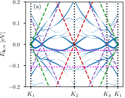
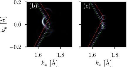
Figure 1: (a) ARPES mapped band structure of tTLG with $\theta_{1}=-0.71^{\circ}$, $\theta_{2}=2.1^{\circ}$ and $\theta_{3}=0^{\circ}$. The bands are shown along the path $\text{K}_{1}\rightarrow\text{K}_{2}\rightarrow\text{K}_{3}\rightarrow\text{K}_{1}$, where $\text{K}_{\ell}$ is the Dirac point of layer $\ell$. The thickness of the blue lines is proportional to $\left|\mathcal{M}_{\mathbf{Q}_{\perp},n}\right|^{2}$, corresponding to the visibility of the bands in ARPES. The dashed lines represent the band structure of the three decoupled graphene layers, following the colour code: layer 1 in green, layer 2 in red, and layer 3 in purple. The horizontal dotted lines mark the energies $\omega=-0.106$ eV and $\omega=-0.028$ eV, which correspond to two van Hove singularities highlighted in Fig. 2. (b) ARPES constant energy map for the same tTLG structure at $\omega=-0.106$ eV. The constant energy map for three decoupled graphene layers is shown in (c) for comparison. The dashed lines represent the Brillouin zone of each layer, following the same colour code as in (a). A broadening of $20$ meV was used.

II.2.3 Total density of states

The total density of states normalized by the total number of states of the trilayer is given by summing over all local density of states

$$\text{TDoS}(\omega)=\frac{1}{\sum_{\ell}N_{\ell}N_{\text{orb}\ell}}\sum_{\ell,\mathbf{R}_{\ell},\alpha}\text{LDoS}_{\ell,\mathbf{R}_{\ell},\alpha}(\omega).$$ (24)

Noticing that sums of the form $\sum_{\mathbf{R}_{1}}e^{i\left(\mathbf{G}_{2}+\mathbf{G}_{3}\right)\cdot\mathbf{R}_{1}}=N_{1}\sum_{\mathbf{G}_{1}}\delta_{\mathbf{G}_{1}+\mathbf{G}_{2}+\mathbf{G}_{3},\mathbf{0}}=N_{1}\delta_{\mathbf{G}_{3},\mathbf{0}}\delta_{\mathbf{G}_{2},\mathbf{0}}$, since for fully incommensurate structures $\mathbf{G}_{1}+\mathbf{G}_{2}+\mathbf{G}_{3}=0$ is only possible if $\mathbf{G}_{1}=\mathbf{G}_{2}=\mathbf{G}_{3}=\mathbf{0}$, we can perform the sums over $\mathbf{R}_{\ell}$’s in Eq. (24) obtaining

$$\text{TDoS}(\omega)=\frac{1}{\sum_{\ell}A_{\text{u.c.}\ell}^{-1}N_{\text{orb}\ell}}\\ \times\sum_{\ell}\int_{\text{BZ}\ell}\frac{d^{2}\mathbf{k}}{\left(2\pi\right)^{2}}\sum_{n,\alpha}\left|\phi_{\ell,\mathbf{k},\alpha}^{n}\left(\mathbf{0},\mathbf{0}\right)\right|^{2}\delta\left(\omega-E_{\mathbf{k},n}\right),$$ (25)

where we used the fact that $N_{\ell}/A=A_{\text{u.c.}\ell}^{-1}$. The contribution from each layer to the total density of states is expressed in terms of an integration over the Brillouin zone of that layer. In the case of a bilayer, the previous result reduces to the one derived in a mathematically rigorous way in Ref. Massatt et al. (2018).

Figure 2: Total and layer resolved density of states for tTLG, with $\theta_{1}=-0.71^{\circ}$, $\theta_{2}=2.1^{\circ}$ and $\theta_{3}=0^{\circ}$. The dot-dashed line shows the total density of states obtained by modelling the tTLG as two tBLG (with the contribution of layer 2 averaged). The two dotted vertical lines mark two van Hove singularities at $\omega=-0.106$ eV and $\omega=-0.028$ eV. The calculation was performed using a mesh of 56677 k points in a circular region of radius $0.043\text{ \r{A}}^{-1}$around the Dirac points of each layer. A broadening of $2$ meV was used.

III Application to twisted trilayer graphene

We now apply the general formalism developed in the previous section to the case of incommensurate tTLG. We model individual layers within the $p_{z}$ orbital, nearest neighbour tight-binding Hamiltonian, with hopping $-t$. For the interlayer coupling we use a Slatter-Koster approximation

$$h_{\alpha\beta}^{\ell\ell^{\prime}}\left(\mathbf{R}_{\ell},\mathbf{R}_{\ell^{\prime}}\right)=V_{pp\pi}\left(R\right)\frac{r^{2}}{R^{2}}+V_{pp\sigma}\left(R\right)\frac{d^{2}}{R^{2}},$$ (26)

where $R=\sqrt{r^{2}+d^{2}}$ is distance between the Wannier centres, with $r=\left|\mathbf{R}_{\ell}+\bm{\tau}_{\ell,\alpha}^{\perp}-\mathbf{R}_{\ell^{\prime}}-\bm{\tau}_{\ell^{\prime},\beta}^{\perp}\right|$ the in-plane distance and $d=3.35\,\text{\r{A}}$ the interlayer separation. The Slatter-Koster functions are parametrized as $V_{pp\pi}\left(R\right)=-te^{-\left(R-a_{\text{CC}}\right)/r_{0}}$ and $V_{pp\sigma}\left(R\right)=t_{\perp}e^{-\left(R-d\right)/r_{0}}$, with $t=2.7$ eV, $t_{\perp}=0.48$ eV, $r_{0}=0.453\,\text{\r{A}}$, and $a_{\text{CC}}=1.42\,\text{\r{A}}$ the intralayer nearest-neighbour distanceMoon and Koshino (2013). Motivated by the recent experimental work of Ref. Zuo et al. (2018), we will focus on a tTLG, where the top layer (layer 1) is rotated by an angle $\theta_{1}=-0.71^{\circ}$, the middle layer (layer 2) is rotated by an angle $\theta_{2}=2.1^{\circ}$ and the bottom layer (layer 3) is taken as the reference, with $\theta_{3}=0^{\circ}$. When constructing the Hamiltonian matrix $\bm{H}_{\mathbf{k}}^{\text{umklapp}}$, we chose a momentum cutoff $\Lambda=2.1\left|\text{K}\right|$, where $\left|\text{K}\right|=4\pi/\left(3\sqrt{3}a_{\text{CC}}\right)$ is the distance of the Dirac points from the origin, such that the first star of reciprocal lattice vectors of each layer is included. In Fig. 1, we shown the computed ARPES mapped band structure and constant energy contour. It is clear that the interlayer coupling leads to a significant reconstruction of the band structure. This is further confirmed if we look at the low energy total density of states, which is shown in Fig. 2. As can be seen the hybridization of layers 1 and 2, and layers 2 and 3 gives origin to two sets of low energy van Hove singularities. However, and differently from what is claimed in Ref. Zuo et al. (2018), the trilayer structure cannot simply be described as two tBLG structures. To show this, in Fig. 2 we also present the total density of states computed by describing the trilayer as two bilayers, with the contribution form layer 2 averaged between the two bilayer systems. As can be seen, there is a significant spectral reconstruction in the trilayer. The presence of the three layers leads to a increased separation between the van Hove singularities of the two bilayer structures. The importance of considering the three layers of the tTLG is also shown when studying the local density of states of the system, which we show in Fig. 3, at the energies corresponding to the van Hove singularities marked in 2. It is clear that the layer resolved LDoS displays a modulation corresponding to the expected moiré pattern due to interference of layer 1 with 3, and layer 2 with 3. However, an additional modulation is observed that corresponds to a moiré pattern due to the interference between layers 1 with 3. This is specially clear in the LDoS of layer 3 at $\omega=-0.106$ eV, which displays a clear modulation with the periodicity of the moiré lattice due to the interference of layers 1 and 3 (whose corresponding lattice is represented by the green star markers). This effect can only be captured if considering coupling between the three layers simultaneously.

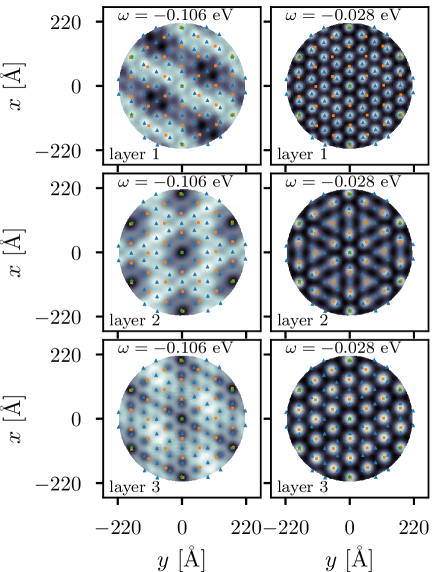
Figure 3: Layer resolved local density of states for tTLG, with $\theta_{1}=-0.71^{\circ}$, $\theta_{2}=2.1^{\circ}$ and $\theta_{3}=0^{\circ}$, at the two van Hove singularities marked by the vertical lines in Fig. 3. Brighter regions correspond to regions with higher density of states. The blue triangles, yellow squares and green stars show, respectivelly, the moiré lattices due to the interference of layers 1 with 2, layers 2 with 3, and layers 1 with 3. The calculation was performed using a mesh of 439 k points in a circular region of radius $0.019\text{ \r{A}}^{-1}$around the Dirac points of each layer. A broadening of $20$ meV was used.

IV Conclusions

In this work, we have developed a tight-binding based, momentum space formalism to describe the electronic properties of incommensurate multilayer van der Waals structures. The method is based on an expansion of the electronic wavefunction in terms of Bloch waves of individual layers, including generalized umklapp scattering due to the competition between the periodicities of the different layers. We also showed how the momentum resolved, local and total density of states, which can be measured via ARPES and STS, can be computed using the developed formalism. Interestingly, both the total and the local density of states can be expressed in terms of integrals over the Brillouin zone of the different layers, a result previously obtained for the total density of states in the bilayer case Massatt et al. (2018). We applied the general formalism to study the spectral properties of tTLG. We found out that the coupling between the three layers can significantly affect the low energy spectral properties, which cannot be simply attributed to the pairwise hybridization between the layers. We found that the low energy van Hove singularities due to the coupling between consecutive layers are repelled due to the hybridization between the three layers. This hybridization between the three layers is also manifested in the modulation of the LDoS, which, besides the moiré patterns due to layers 1 with 2, and layers 2 with 3, also display a modulation due to the hybridization between layers 1 with 3. The formalism developed in this paper is capable of describing structures with arbitrary lattice mismatch and misalignment. Its flexibility makes it very promising to study spectral and transport properties of the technologically relevant graphene/boron nitride/graphene and graphene/STMD/graphene structures.